A Controller Design Based on Takagi-Sugeno Fuzzy Model Employing Trajectory of Partial Uncertainty

Abstract

When the Takagi–Sugeno (T-S) fuzzy model is used to design controllers for a concerned system, the discrepancy between the system and its T-S fuzzy model becomes crucial sometimes in terms of control performance, particularly in cases when the magnitude of the discrepancy is relatively large. While most existing works have focused on approaches to restrain the influence of the discrepancy, the idea used in this paper is to extract as much information from the discrepancy as possible at first and then use it in the controller design before restraining its influence. By doing so, the magnitude of the discrepancy is reduced accordingly, and thus, better control performance can be expected. Including the discrepancy and other uncertain elements like the inner parameters’ perturbation, a term called uncertainty is considered in this paper. Assuming that the uncertainty influences the system behavior through the state and control input, an observer able to catch the trajectory of the partial uncertainty related to the control input is proposed. Then, a controller employing the trajectory is suggested. All design parameters are obtained by solving certain linear matrix inequalities, which guarantees the system stability. Finally, simulations are provided to illustrate the effectiveness of the proposed approach.

1. Introduction

The Takagi–Sugeno (T-S) fuzzy model [1] is composed of certain If-Then fuzzy rules, in which each consequent part is in the form of the state-space representation that is a linear differential equation. Though the overall T-S fuzzy model is a nonlinear model (meaning a nonlinear differential equation), techniques for controller design based on linear models such as linear feedback control can still be applied, if a controller design based on the T-S fuzzy model is developed using the concept of the so-called parallel distributed compensation (PDC). This is one of the main reasons why there have been significant advances in the study of the stability analysis and controller synthesis based on the T-S fuzzy model since the beginning of the 1990s. In particular, with the help of some advanced software packages such as the third-party MATLAB toolbox, the design parameters in the PDC controller can be numerically obtained by solving certain linear matrix inequalities (LMIs) that provide sufficient conditions for system stability in the sense of Lyapunov stability.

On the other hand, the T-S fuzzy model, like other models, in most cases, is comprised of approximate mathematical expressions for the purpose of designing a controller for the system. This means that there is a discrepancy between a real system and its T-S fuzzy model. Including the discrepancy, this paper uses a term called uncertainty to express the unmodeled dynamics such as external/internal disturbance and parameter perturbations beyond the T-S fuzzy model. If the uncertainty is small enough, i.e., the T-S fuzzy model matches the real system perfectly well, the control performance of the controller based on the T-S fuzzy model will be as good as designed; however, in the case when the magnitude of the uncertainty is relatively large, the controller may not work well when it is applied to the real system, and in the worst case, the closed-loop system may become unstable. Therefore, in order to guarantee and improve the control performance, the uncertainty must be taken into consideration in the T-S fuzzy model.

Though the uncertainty is referred to by different names in different contexts, how to deal with it has been a very typical subject in control systems. Among the existing approaches, $H_{\infty }$ control [2,3,4,5,6] is an effective approach that keeps the ratio of the influence from the uncertainty on the real system below some prescribed indexes. Though a wide range of related works was reported, as a result, the influence from the uncertainty becomes larger accordingly if the magnitude of the uncertainty is larger, even if the ratio is kept the same. Another way to handle the uncertainty in the T-S fuzzy model is to utilize the capability of the fuzzy approximator capable of uniformly approximating unknown nonlinearities [7,8,9,10], in which related parameters are tuned by adaptive laws [2]. However, the parameters lying in the fuzzy approximators are tuned on the basis, not of the improvement of the approximateness, but of the system stability. In other words, if the approximateness is not guaranteed, the control performance cannot be as good as expected, and even the overall control system becomes unstable in the worst case.

Assuming the uncertainty is norm-bounded with certain structures in the T-S fuzzy model, some works involved certain known matrices defining the norm-bounded uncertainty in certain LMIs, which guarantees the system stability [11,12,13,14]. However, it is not easy to estimate the norm-bounded matrices because the mathematical model of the real system is unavailable in most cases; thus, the magnitudes of the norm-bounded matrices are often set large to safely cover the uncertainty, which results in conservative stability conditions. On the other hand, viewing the uncertainty as an unknown input, there are existing approaches of designing state observers decoupling the influence of the unknown input in the field of fault diagnosis [15,16,17]. However, when further designing a controller based on the model with unknown input, in fact, the approach used in the design of the state observers cannot be applied straightforwardly to the design of controller.

Uncertainty observer-based control provides a promising approach to handle system uncertainty and improve robustness [18,19,20,21]. In this framework, a baseline controller is first designed under the assumption that the uncertainty is not considered, and then, a compensation part is added to the baseline controller in order to counteract the influence of the uncertainty that is estimated by an observer. However, all the proposed observers are designed on the assumption that the uncertainty only lies in the control matrices and must not be time-dependent, which clearly limits its applications.

While it is difficult to estimate the uncertainty itself particularly when it is highly oscillating, the paper makes an effort to extract as much information from the uncertainty as possible; then, the information is utilized in the controller design. Consequently, the influence of the uncertainty will be reduced accordingly, which leads to a better control performance. In the T-S fuzzy model considered in this paper, the uncertainty is thought to influence the system behavior through the state and the control input. While the former part of the uncertainty is assuming norm-boundedness, this paper focuses attention on the latter part of the uncertainty, because it is linked to the control input directly, which implies that any information available about the uncertainty can be used directly, as well. Concretely, the latter part of the uncertainty is virtually divided further into a constant part and a time-varying part, and an observer of the constant part is designed. As a result, the observer is able to catch the trajectory of the latter part of the uncertainty. Following the observer design, a controller using the information of the trajectory from the observer is proposed, in which the conditions guaranteeing the system stability are arranged in the form of LMIs. Finally, simulation results are provided to illustrate the effectiveness of the approach proposed in this paper.

2. T-S Fuzzy Model and Partial Disturbance Observer

Assume that a nonlinear system can be represented by the following T-S fuzzy model [1]:

$$\begin{array}{c}\mathrm{Plant}\mathrm{Rule}i:\hfill \\ \mathrm{If}{\theta }_1\left(t\right)\mathrm{is}{M}_1^i\mathrm{and}\cdots \mathrm{and}{\theta }_{n_{\theta }}\left(t\right)\mathrm{is}{M}_{n_{\theta }}^i,\mathrm{Then}\hfill \\ \left.\begin{array}{c}\dot{x}\left(t\right)=A_{i}x\left(t\right)+B_{i}u\left(t\right)+F_i\left(t\right)\hfill \\ y\left(t\right)=C_{i}x\left(t\right)\hfill \\ \dot{y}\left(t\right)=C_i\dot{x}\left(t\right)\hfill \end{array}\right\}\hfill \end{array}$$

(1)

where ${\theta }_j(j=1,2,\cdots ,n_{\theta })$ is a variable in the antecedent that is available; $M_j^i(i=1,2,\dots ,n_r)$, a fuzzy term corresponding to the i-th rule; $x\left(t\right)\in R^n$, the state vector; $u\left(t\right)\in R^m$, the input vector; $y\left(t\right)\in R^p$, the output vector; $A_i\in R^{n\times n}$, $B_i\in R^{n\times m}$, $C_i\in R^{p\times n}$, some compatible matrices; $F_i\left(t\right)\in R^n$, uncertainty including modeling error, external disturbance, unmodeled dynamics and parameter perturbations.

The overall T-S fuzzy model is of the following form accordingly:

$$\begin{array}{c}\left.\begin{array}{c}\dot{x}\left(t\right)={\sum }_{i=1}^{n_r}{\alpha }_i\left(t\right)\left(A_{i}x\left(t\right)+B_{i}u\left(t\right)+F_i\left(t\right)\right)\hfill \\ y\left(t\right)={\sum }_{i=1}^{n_r}{\alpha }_i\left(t\right)C_{i}x\left(t\right)\hfill \\ \dot{y}\left(t\right)={\sum }_{i=1}^{n_r}{\alpha }_i\left(t\right)C_i\dot{x}\left(t\right)\hfill \end{array}\right\}\end{array}$$

(2)

where $\theta \left(t\right)=\left[{\theta }_1\left(t\right){\theta }_2\left(t\right)\cdots {\theta }_{n_{\theta }}\left(t\right)\right]$,

$$\begin{array}{ccc}{\alpha }_i\left(t\right)=\frac{{\omega }_i\left(\theta \left(t\right)\right)}{{\sum }_{i=1}^{n_r}{\omega }_i\left(\theta \left(t\right)\right)}\ge 0,\hfill & \hfill \sum _{i=1}^{n_r}{\alpha }_i\left(t\right)=1,& \hfill {\omega }_i\left(\theta \left(t\right)\right)=\prod _{j=1}^{n_{\theta }}{M}_j^i\left({\theta }_j\left(t\right)\right).\end{array}$$

At first glance, $\dot{y}\left(t\right)=C_i\dot{x}\left(t\right)$ in (1) seems redundant due to the fact that it can be obtained directly from $y\left(t\right)=C_{i}x\left(t\right)$. However, when it comes to the fuzzy inference, $\dot{y}\left(t\right)={\sum }_{i=1}^{n_r}{\alpha }_i\left(t\right)C_i\dot{x}\left(t\right)$ in (2) cannot be obtained straightforwardly from $y\left(t\right)={\sum }_{i=1}^{n_r}{h}_i\left(t\right)C_{i}x\left(t\right)$, which leads to:

$$\begin{array}{c}\dot{y}\left(t\right)=\sum _{i=1}^{n_r}{\dot{\alpha }}_i\left(t\right)C_{i}x\left(t\right)+\sum _{i=1}^{n_r}{\alpha }_i\left(t\right)C_i\dot{x}\left(t\right).\end{array}$$

Therefore, we assume that in this paper, ${\sum }_{i=1}^{n_r}{\dot{\alpha }}_i\left(t\right)C_{i}x\left(t\right)=0$ in order to focus our attention on simple control approaches rather than complex formula manipulation. In addition, if $C_1=C_2=\cdots =C_{n_r}=C$ as in most cases of the T-S fuzzy models, then $\dot{y}\left(t\right)=C_i\dot{x}\left(t\right)$ is no longer needed due to the fact that $y\left(t\right)={\sum }_{i=1}^{n_r}{\alpha }_i\left(t\right)C_{i}x\left(t\right)=Cx\left(t\right)$, which leads to $\dot{y}\left(t\right)=C\dot{x}\left(t\right)$.

As for the uncertainty $F_i\left(t\right)$, we assume it influences the system behavior through the state and the control input:

$$\begin{array}{c}{F}_i\left(t\right)=\Delta A_i\left(t\right)x\left(t\right)+B_i\Delta u_i\left(t\right),\end{array}$$

(3)

where $\Delta A_i\left(t\right)$ denotes a partial influence of the uncertainty on the state $x\left(t\right)$, while $\Delta u_i\left(t\right)$ represents a further partial influence of the uncertainty on the control input $u\left(t\right)$.

Paying attention to $\Delta u_i\left(t\right)$, which influences the system through the control matrix $B_i$ the same as the control input $u\left(t\right)$, it is reasonable to consider that it would be able to design a controller that is based on a regular control input $u\left(t\right)$ with an extra element such as $u\left(t\right)-\Delta u_i\left(t\right)$ to counteract the influence of $\Delta u_i\left(t\right)$ completely if $\Delta u_i\left(t\right)$ were available. While it is impossible to catch the real value of $\Delta u_i\left(t\right)$ as a whole, it is still desirable to employ some information of $\Delta u_i\left(t\right)$, even partially, to counteract its influence on the system as much as possible. On the other hand, some existing works have shown that we are able to estimate $\Delta u_i\left(t\right)$ under the condition of $\frac{d}{dt}\Delta u_i\left(t\right)=0$ [22,23], which means that $\Delta u_i\left(t\right)$ must be a constant, or precisely, not a time-dependent function. Though such a condition is evidently strict from the point of view of dynamic control systems, in fact, as pointed out by Wu and Han [23], the condition can, not theoretically, but practically, be extended to cases such as the piecewise-constant case and the slowly time-varying case (${\dot{d}}_c\left(t\right)\simeq 0$). However, when it comes to a sharply time-varying case, it is clear that the condition cannot be tolerated anymore.

On the basis of the aforementioned observation, we virtually divide $\Delta u_i\left(t\right)$ into a constant part $d_c$ and a time-vary part $\Delta d_i\left(t\right)$:

$$\begin{array}{c}\Delta u_i\left(t\right)=d_c+\Delta d_i\left(t\right).\end{array}$$

(4)

Whether $\Delta d_i\left(t\right)$ is either slowly time-varying or sharply time-varying, we assume it, along with $\Delta A_i\left(t\right)$, is norm-bounded as follows [11]:

$$\begin{array}{c}\hfill \left[\begin{array}{cc}\Delta A_i\left(t\right)& 0\\ 0& \Delta d_i\left(t\right)\end{array}\right]=\left[\begin{array}{cc}{M}_{Ai}& 0\\ 0& M_{di}\end{array}\right]{\mathrm{\Theta }}_i\left(t\right)\left[\begin{array}{cc}{N}_A& 0\\ 0& N_d\end{array}\right],\end{array}$$

(5)

where $M_{Ai},M_{di},N_A$ and $N_d$ are known constant matrices with compatible dimensions and ${\mathrm{\Theta }}_i\left(t\right)$ is an unknown nonlinear time-varying matrix function satisfying:

$$\begin{array}{c}{\mathrm{\Theta }}_i\left(t\right){\mathrm{\Theta }}_i{\left(t\right)}^T\le I.\end{array}$$

(6)

Regarding the virtually constant part $d_c$ in (4), we use the following observer to estimate it:

$$\begin{array}{c}\mathrm{Observer} \mathrm{Rule}i:\hfill \\ \mathrm{If}{\theta }_1\left(t\right)is{M}_1^{i}and\cdots \mathrm{and}{\theta }_p\left(t\right)\mathrm{is}{M}_p^i,\mathrm{Then}\hfill \\ \left.\begin{array}{c}{\widehat{d}}_c\left(t\right)=\xi \left(t\right)+Ly\left(t\right)\hfill \\ \dot{\xi }\left(t\right)=-L{\sum }_{j=1}^{n_r}{\alpha }_j\left(t\right)C_j\left(A_{i}x\left(t\right)+B_i(u\left(t\right)+{\widehat{d}}_c\left(t\right))\right)\hfill \end{array}\right\}\hfill \end{array}$$

(7)

where ${\widehat{d}}_c\in R^m$ is the estimate of the constant part $d_c$; $\xi \in R^m$, the internal state vector of the observer; $L\in R^{m\times r}$, the observer gain to be determined. The overall observer is of the following form accordingly:

$$\begin{array}{c}\left.\begin{array}{c}{\widehat{d}}_c\left(t\right)=\xi \left(t\right)+Ly\left(t\right)\hfill \\ \dot{\xi }\left(t\right)=-{\sum }_{i=1}^{n_r}{\sum }_{j=1}^{n_r}{\alpha }_i\left(t\right){\alpha }_j\left(t\right)L{C}_j\left(A_{i}x\left(t\right)+B_i(u\left(t\right)+{\widehat{d}}_c\left(t\right))\right)\hfill \end{array}\right\}.\end{array}$$

(8)

Defining the estimation error between $d_c$ and ${\widehat{d}}_c$ as:

$$\begin{array}{c}\hfill e_d=d_c-{\widehat{d}}_c,\end{array}$$

(9)

we have:

$$\begin{array}{cc}\hfill {\dot{e}}_d& =-\dot{\xi }-L\dot{y}\hfill \\ \hfill & =\sum _{i=1}^{n_r}\sum _{j=1}^{n_r}{\alpha }_i{\alpha }_{j}L{C}_j\left(A_{i}x+B_i(u+{\widehat{d}}_c)\right)-\sum _{i=1}^{n_r}\sum _{j=1}^{n_r}{\alpha }_i{\alpha }_{j}L{C}_j\left((A_i+\Delta A_i)x+B_i(u+d_c+\Delta d_i)\right)\hfill \\ \hfill & =-\sum _{i=1}^{n_r}\sum _{j=1}^{n_r}{\alpha }_i{\alpha }_{j}L{C}_j\left(B_i{e}_d+\Delta A_{i}x+B_i\Delta d_i\right),\hfill \end{array}$$

(10)

where the facts that $\dot{y}\left(t\right)={\sum }_{i=1}^{n_r}{\alpha }_i\left(\theta \right)C_i\dot{x}\left(t\right)$ and ${\dot{d}}_c=0$ are used. It is worth noting that ${\dot{d}}_c=0$ is not an assumption in this paper, because $d_c$ is considered as the constant part in (4).

Before starting the controller design, the following lemma is first provided, which will be used in the control system stability analysis [24].

Lemma 1.

Given matrices A, M, E and $R=R^T>0$ with appropriate dimensions, let $\mathrm{\Theta }\left(t\right)$ be of the appropriate dimensions and satisfy $\mathrm{\Theta }{\left(t\right)}^T\mathrm{\Theta }\left(t\right)\le I$. Then, the following holds:

(a) 

For any scalar $ϵ>0$,

$$\begin{array}{c}M\mathrm{\Theta }\left(t\right)E+{\left(M\mathrm{\Theta }\left(t\right)E\right)}^T\le ϵM{M}^T+{ϵ}^{-1}{E}^{T}E.\end{array}$$

(11)

(b) 

If for some constant $ϵ>0$ such that $ϵI-ER{E}^T>0$, then:

$$\begin{array}{c}(A+M\theta \left(t\right)E)R{(A+M\theta \left(t\right)E)}^T\le AR{(R-{ϵ}^{-1}R{E}^{T}ER)}^{-1}R{A}^T+ϵM{M}^T\end{array}$$

(12)

or:

$$\begin{array}{c}(A+M\theta \left(t\right)E)R{(A+M\theta \left(t\right)E)}^T\le AR{A}^T+AR{E}^T{(ϵI-ER{E}^T)}^{-1}ER{A}^T+ϵM{M}^T.\end{array}$$

(13)

From here, unless confusion arises, arguments such as t and $\theta$ will be omitted just for notational convenience. An asterisk (∗) for inline expressions denotes the transpose of the terms on its left-hand side; for matrix expressions, it denotes the transpose of its symmetric block-entry.

3. Controller Design

Based on the partial disturbance observer, the following PDC controller is proposed.

$$\begin{array}{c}\mathrm{Controller} \mathrm{Rule}i:\hfill \\ \mathrm{If}{\theta }_1\mathrm{is}{M}_1^i\mathrm{and}\cdots \mathrm{and}{\theta }_p\mathrm{is}{M}_p^i,\mathrm{Then}\hfill \\ u=K_{i}x-{\widehat{d}}_c\hfill \end{array}$$

(14)

where $K_i\in R^{m\times n}$ is the control gain to be determined. Compared to the regular PDC controller, there is an extra term ${\widehat{d}}_c$ in order to counteract the disturbance whenever possible. The overall PDC controller is of the following form accordingly:

$$\begin{array}{c}u=\sum _{i=1}^{n_r}{\alpha }_i{K}_{i}x-{\widehat{d}}_c.\end{array}$$

(15)

Substituting (15) into (2), the closed-loop control system becomes:

$$\begin{array}{cc}\hfill \dot{x}=& \sum _{i=1}^{n_r}\sum _{j=1}^{n_r}{\alpha }_i{\alpha }_j\left((A_i+\Delta A_i)x+B_i(K_{j}x-\widehat{d_c}+d_c+\Delta d_i)\right)\hfill \\ \hfill =& \sum _{i=1}^{n_r}\sum _{j=1}^{n_r}{\alpha }_i{\alpha }_j\left((A_{i}x+B_i{K}_j)x+\Delta A_{i}x+B_i{e}_d+B_i\Delta d_i\right).\hfill \end{array}$$

(16)

Combining (A5) with (A7), we have the following augmented system containing the state and estimation error of the partial disturbance:

$$\begin{array}{c}\hfill {\dot{x}}_e=\sum _{i=1}^{n_r}\sum _{j=1}^{n_r}{\alpha }_i{\alpha }_j\left({\mathcal{A}}_{ij}{x}_e+\Delta {\mathcal{A}}_{ij}{x}_e+{\mathcal{B}}_{ij}\Delta d_i\right),\end{array}$$

(17)

where:

$$\begin{array}{cccc}\hfill x_e=\left[\begin{array}{c}x\\ e_d\end{array}\right],& {\mathcal{A}}_{ij}=\left[\begin{array}{cc}{A}_i+B_i{k}_j& B_i\\ 0& -L{C}_j{B}_i\end{array}\right],\hfill & \hfill \Delta {\mathcal{A}}_{ij}=\left[\begin{array}{cc}\Delta A_i& 0\\ -L{C}_j\Delta A_i& 0\end{array}\right],& {\mathcal{B}}_{ij}=\left[\begin{array}{c}{B}_i\\ -L{C}_j{B}_i\end{array}\right].\hfill \end{array}$$

(18)

The stability of the above augmented closed-loop system is investigated based on the Lyapunov stability theory. Let us consider the following quadratic Lyapunov function candidate:

$$\begin{array}{c}V=x_e^{T}P{x}_e\end{array}$$

(19)

where:

$$\begin{array}{c}P=\left[\begin{array}{cc}{P}_1& 0\\ 0& P_2\end{array}\right]>0,\end{array}$$

(20)

$P_1=P_1^T$, $P_2=P_2^T$.

Taking the time derivative of V, we have:

$$\begin{array}{cc}\hfill \dot{V}=& {\dot{x}}_e^{T}P{x}_e+x_e^{T}P\dot{x_e}\hfill \\ \hfill =& \sum _{i=1}^{n_r}\sum _{j=1}^{n_r}{\alpha }_i{\alpha }_j\{\left(x_e^T{\mathcal{A}}_{ij}^T+x_e^T\Delta {\mathcal{A}}_i^T+\Delta d_i^T{\mathcal{B}}_{ij}^T\right)P{x}_e+x_e^{T}P\left({\mathcal{A}}_{ij}{x}_e+\Delta {\mathcal{A}}_i{x}_e+{\mathcal{B}}_{ij}\Delta d_i\right)\hfill \\ \hfill =& \sum _{i=1}^{n_r}\sum _{j=1}^{n_r}{\alpha }_i{\alpha }_j{x}_e^T\left({\mathcal{A}}_{ij}^{T}P+P{\mathcal{A}}_{ij}\right)x_e+2x_e^{T}P\Delta {\mathcal{A}}_{ij}{x}_e+2x_e^{T}P{\mathcal{B}}_{ij}\Delta d_i.\hfill \end{array}$$

(21)

Substituting the following inequalities into (21),

$$\begin{array}{cc}\hfill 2P\Delta {\mathcal{A}}_{ij}& =2P\left[\begin{array}{cc}\Delta A_i& 0\\ -L{C}_j\Delta A_i& 0\end{array}\right]\hfill \\ \hfill & =2P\left[\begin{array}{c}I\\ -L{C}_j\end{array}\right]\Delta A_i\left[\begin{array}{cc}I& 0\end{array}\right]\hfill \\ \hfill & =2P\left[\begin{array}{c}I\\ -L{C}_j\end{array}\right]M_{A_i}{\mathrm{\Theta }}_i{N}_A\left[\begin{array}{cc}I& 0\end{array}\right]\hfill \\ \hfill & \le P\left[\begin{array}{c}I\\ -L{C}_j\end{array}\right]M_{A_i}{M}_{A_i}^T{\left[\begin{array}{c}I\\ -L{C}_j\end{array}\right]}^{T}P+{\left[\begin{array}{cc}I& 0\end{array}\right]}^T{N}_A^T{N}_A\left[\begin{array}{cc}I& 0\end{array}\right]\hfill \\ \hfill & =P{\mathcal{M}}_{ij}{\mathcal{M}}_{ij}^{T}P+{\mathcal{N}}_i,\hfill \end{array}$$

(22)

where:

$$\begin{array}{cccc}\hfill {\mathcal{M}}_{ij}& =\left[\begin{array}{c}{M}_{A_i}\\ -L{C}_j{M}_{A_i}\end{array}\right],\hfill & \hfill {\mathcal{N}}_i& =\left[\begin{array}{cc}{N}_A^T{N}_A& 0\\ 0& 0\end{array}\right],\hfill \end{array}$$

(23)

and:

$$\begin{array}{cc}\hfill 2x_e^{T}P{\mathcal{B}}_{ij}\Delta d_i& =2x_e^{T}P{\mathcal{B}}_{ij}{M}_{d_i}{\mathrm{\Theta }}_i{N}_d\hfill \\ \hfill & \le x_e^{T}P{\mathcal{B}}_{ij}{M}_{d_i}{M}_{d_i}^T{\mathcal{B}}_{ij}^{T}P{x}_e+N_d^T{N}_d,\hfill \end{array}$$

(24)

where (a) of Lemma 1 is used, we have:

$$\begin{array}{cc}\hfill \dot{V}\le & \sum _{i=1}^{n_r}\sum _{j=1}^{n_r}{\alpha }_i{\alpha }_j\left\{x_e^T\left({\mathcal{A}}_{ij}^{T}P+P{\mathcal{A}}_{ij}+P{\mathcal{M}}_{ij}{\mathcal{M}}_{ij}^{T}P+{\mathcal{N}}_i+P{\mathcal{B}}_{ij}{M}_{d_i}{M}_{d_i}^T{\mathcal{B}}_{ij}^{T}P\right)x_e+N_d^T{N}_d\right\}.\hfill \end{array}$$

(25)

Letting:

$$\begin{array}{c}{\mathcal{A}}_{ij}^{T}P+P{\mathcal{A}}_{ij}+P{\mathcal{M}}_{ij}{\mathcal{M}}_{ij}^{T}P+{\mathcal{N}}_i+P{\mathcal{B}}_{ij}{M}_{d_i}{M}_{d_i}^T{\mathcal{B}}_{ij}^{T}P\le -\eta I\end{array}$$

(26)

where $\eta >0$ is a prescribed constant, from (25), we have:

$$\begin{array}{cc}\hfill \dot{V}& \le -\sum _{i=1}^{n_r}\sum _{j=1}^{n_r}{\alpha }_i{\alpha }_j{x}_e^T\eta x_e+N_d^T{N}_d\hfill \\ \hfill & =-x_e^T\eta x_e+N_d^T{N}_d\hfill \\ \hfill & =-\eta x_e^T{x}_e{\gamma }_{max}^{-1}\left(P\right){\gamma }_{max}\left(P\right)+N_d^T{N}_d\hfill \\ \hfill & \le -\eta {\gamma }_{max}^{-1}\left(P\right)x_e^{T}P{x}_e+N_d^T{N}_d\hfill \\ \hfill & =-\eta {\gamma }_{max}^{-1}\left(P\right)V+N_d^T{N}_d\hfill \\ \hfill & =-\kappa V+N_d^T{N}_d,\hfill \end{array}$$

(27)

where ${\gamma }_{max}\left(P\right)>0$ is the maximum eigenvalue of P, $\kappa =\eta {\gamma }_{max}^{-1}\left(P\right)>0$. Considering the relation in (5) and $\Delta d_i\in R^{m\times 1}$, whatever the dimensions of $M_{di}$ and ${\mathrm{\Theta }}_i$ may be, $N_d$ must be a vertical vector. As a result, $N_d^T{N}_d$ is a scalar.

From (27), we have:

$$\begin{array}{c}V\left(t\right)\le e^{-\kappa t}\left(V\left(0\right)-\frac{N_d^T{N}_d}{\kappa }\right)+\frac{N_d^T{N}_d}{\kappa },\end{array}$$

(28)

which implies that after sufficient time has elapsed, $e^{-\kappa t}\left(V\left(0\right)-\frac{N_d^T{N}_d}{\kappa }\right)$ will tend to zero, i.e.,

$$\begin{array}{c}V\le \frac{N_d{N}_d^T}{\eta }{\gamma }_{max}\left(P\right).\end{array}$$

(29)

Considering the relation of $V=x_e^{T}P{x}_e\ge \parallel x_e{\parallel }^2{\gamma }_{min}\left(P\right)$, where ${\gamma }_{min}\left(P\right)>0$ is the minimum eigenvalue of P, from (29), we have:

$$\begin{array}{c}\parallel x_e\parallel \le \sqrt{\frac{N_d{N}_d^T{\gamma }_{max}\left(P\right)}{\eta {\gamma }_{min}\left(P\right)}}.\end{array}$$

(30)

Therefore, the problem left is how to maintain the inequality (26). By the Schur complement, (26) is equivalent to the following:

$$\begin{array}{c}\left[\begin{array}{ccc}P{\mathcal{A}}_{ij}+(\ast )+{\mathcal{N}}_i+\eta I& P{\mathcal{M}}_{ij}& P{\mathcal{B}}_{ij}{M}_{d_i}\\ \ast & -I& 0\\ \ast & \ast & -I\end{array}\right]<0.\end{array}$$

(31)

Substituting (18) and (23) into (31), we have:

$$\begin{array}{c}\left[\begin{array}{cccc}\Xi & P_1{B}_i& P_1{M}_{A_i}& P_1{B}_i{M}_{d_i}\\ \ast & -F{C}_j{B}_i-(\ast )+\eta I& -F{C}_j{M}_{A_i}& -F{C}_j{B}_i{M}_{d_i}\\ \ast & \ast & -I& 0\\ \ast & \ast & \ast & -I\end{array}\right]<0.\end{array}$$

(32)

where $F=P_{2}L\in R^{m\times r}$,

$$\begin{array}{c}\Xi =P_1{A}_i+P_1{B}_i{K}_j+(\ast )+\left(N_A^T{N}_A+\eta \right)I\end{array}$$

(33)

Considering that $P_1$, $K_j$, F and $P_2$, which is hidden in F, are parameters to be determined, $\Xi$ is nonlinear. Though, except $\Xi$, the other blocks are all linear, (32) cannot be treated as an LMI issue to obtain the parameters satisfying the inequality. However, bearing in mind that a necessary condition to hold the inequality is the leading principal minor $\Xi <0$, here in this paper, we first consider obtaining $K_j$ such that:

$$\begin{array}{c}\left.\begin{array}{c}{Q}_1>0\hfill \\ \left[\begin{array}{cc}{A}_i{Q}_1+B_i{M}_j+(\ast )& Q_1\\ \ast & -{(N_A^T{N}_A+\eta )}^{-1}I\end{array}\right]<0\hfill \end{array}\right\},i,j=1,2,\dots ,n_r\end{array}$$

(34)

where $Q_1=Q_1^T=P_1^{-1},M_j=K_j{Q}_1$. It is evident that by the Schur complement, $\Xi <0$ holds if (34) is satisfied. By solving LMIs in (34), we have:

$$\begin{array}{c}{K}_j=M_j{Q}_1^{-1}.\end{array}$$

(35)

Once $K_j$ is known, (32) becomes LMIs. In other words, viewing $P_1,P_2$, F as the decision variables, solving (32) along with LMI (20), the observer gain L can be obtained as follows.

$$\begin{array}{c}L=P_2^{-1}F.\end{array}$$

(36)

To sum up all results above, the following theorem is provided.

Theorem 1.

Consider a nonlinear system represented by the T-S fuzzy model (2) with the uncertainty $F_i$ subject to (3)–(6), the partial uncertainty observer (7) and controller (15) in which the observer gain L and the control gain $K_j$ ($j=1,\dots ,n_r$) are obtained by the following two steps. For a prescribed scalar $\eta >0$, if there exists symmetric matrices $P_1,P_2,Q_1$, matrices F and $M_j$ with appropriate dimensions obtained progressively:

Step 1 

solving LMIs (34) to obtain $Q_1,M_j$, then $K_j$ by (35),

Step 2 

solving LMIs (20) and (32) to obtain $P_1,P_2$ and F, then L by (36), where $K_j$ is known by Step 1,

then the augmented system $x_e$ containing the state x and the estimation error of the partial disturbance defined in (9) will remain stable, and the state $x_e$ will converge to the region defined in (30).

Regarding this theorem, we give the following remarks.

Remark 1.

It follows from (30) that it is better to set a larger η and a smaller $N_d$ in order to make $\parallel x_e\parallel$ smaller. However, a larger η leads to LMIs (34) tending to be more difficult to satisfy, while a smaller $N_d$ causes the risk that $\Delta d_i$ is no longer covered by $M_{d_i}{\mathrm{\Theta }}_i{N}_d$, as shown in (5). There is a trade-off between the parameter setting and the convergence.

Remark 2.

$P_2$ is not involved in the LMIs (32) directly in Step 2, which implies that it is enough as long as $P_2>0$ as required by the LMI (20). Therefore, from (36), we observe that a smaller $P_2$ leads to a larger observer gain L. In order to adjust the magnitude of $P_2$,

$$\begin{array}{c}\left[\begin{array}{cc}{P}_1& 0\\ 0& \gamma P_2\end{array}\right]>0,\end{array}$$

(37)

where $\gamma >0$ is set manually.

Remark 3.

The theorem is based on the condition that the state x is available. A similar design is provided in Appendix A in the case that the state is unavailable.

4. Simulation

Consider the following altered Van der Pol oscillator [25]:

$$\begin{array}{c}\hfill \left.\begin{array}{c}\left[\begin{array}{c}{\dot{x}}_1\\ {\dot{x}}_2\end{array}\right]=\left[\begin{array}{c}\left(1+0.5sin\left(t\right)\right)x_2\\ -x_1+\left(1-x_1^2\right)x_2+u\end{array}\right]+F\hfill \\ y=x_2\hfill \end{array}\right\}\end{array}$$

(38)

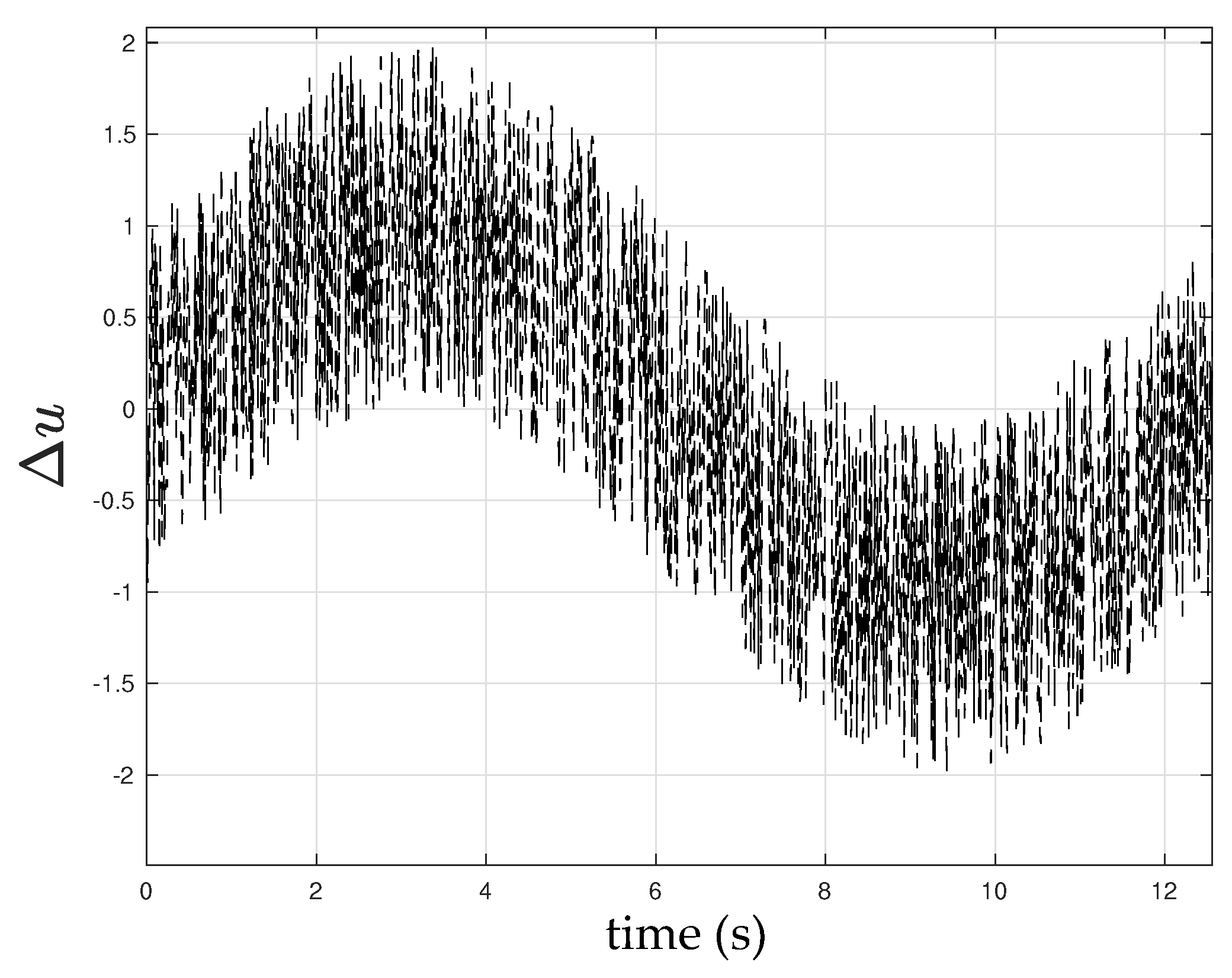
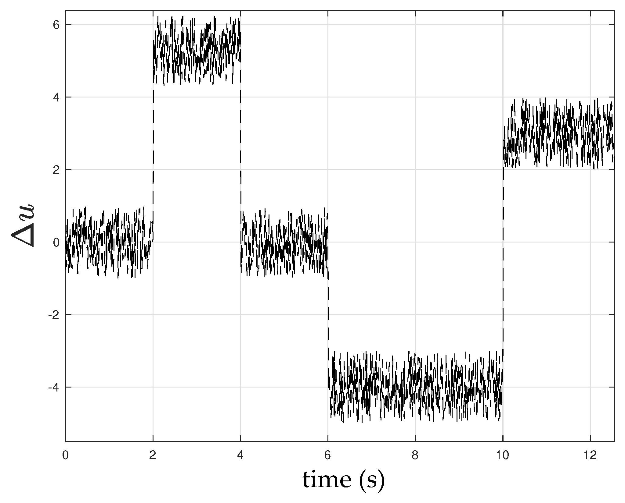
where the uncertainty in (3) is given as:

$$\begin{array}{c}\hfill F=\left[\begin{array}{cc}0& 0.5sin\left(t\right)\\ 0& 0\end{array}\right]x+\left[\begin{array}{c}0\\ 1\end{array}\right]\Delta u,\end{array}$$

(39)

and $x^T=\left[x_1{x}_2\right]$, in which $\Delta u$ is considered in two cases that are depicted in Figure 1 and Figure 2.

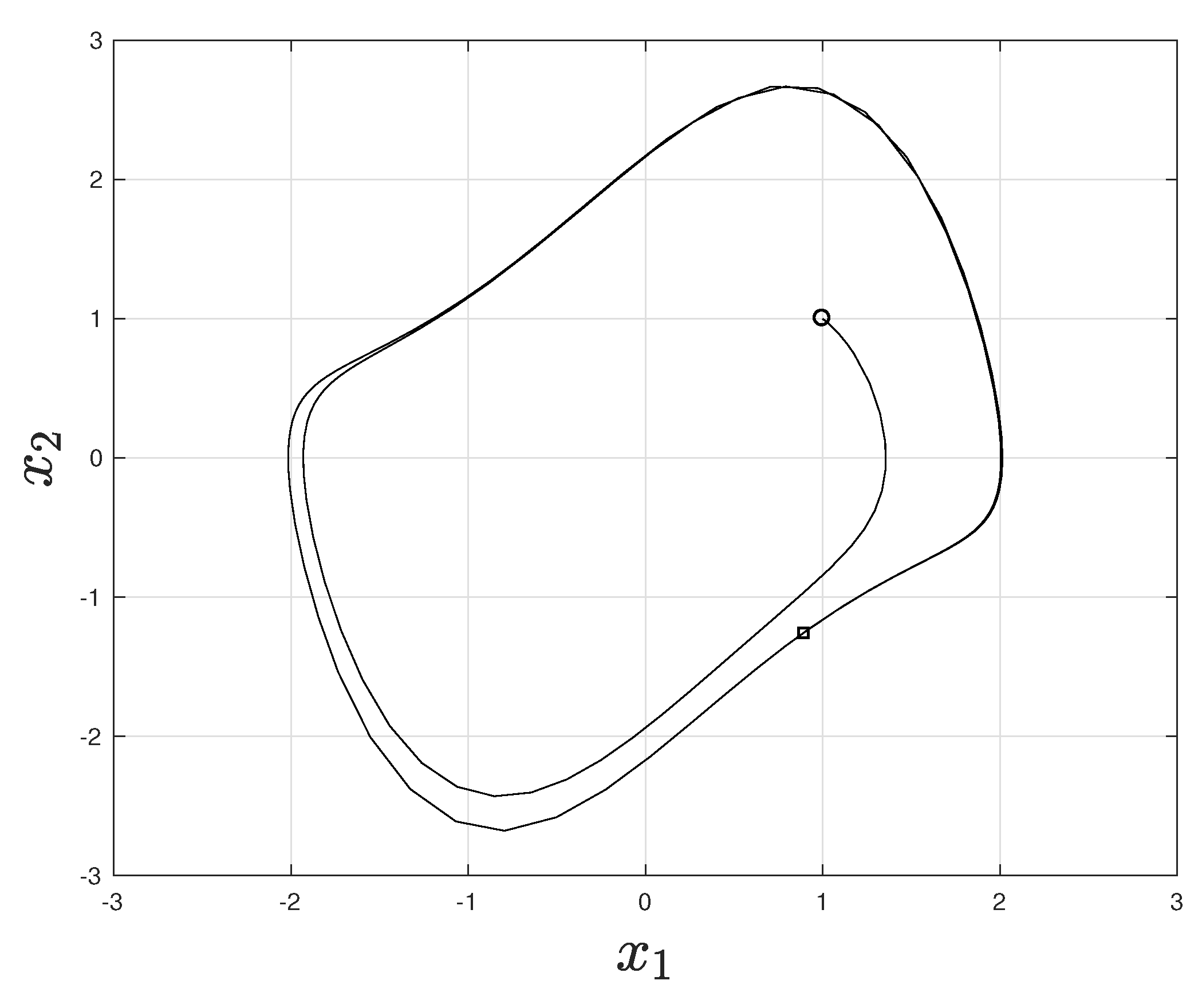
Without control and uncertainty, i.e., $u=0$ and $\Delta F=0$, the $x_1-x_2$ phase plane is shown in Figure 3, where the circle is the initial point and the square is the end point. It is clear that the unforced system is unstable.

The above nonlinear system can be represented by the following two-rule T-S fuzzy model:

$$\begin{array}{cc}\hfill \mathrm{Rule}i:& \mathrm{If}{x}_1\mathrm{is}{M}^i\left(x_1\right),\mathrm{Then}\hfill \\ \hfill & \left.\begin{array}{c}\dot{x}=\left(A_i+\Delta A_i\right)x+B_i\left(u+\Delta u\right)\hfill \\ y=C_{i}x\hfill \end{array}\right\}\hfill \end{array}$$

(40)

where $i=1,2$, $M^1\left(x_1\right)=\left\{\begin{array}{cc}\frac{9-x_1^2}{9},\hfill & -3\le x_1\le 3\hfill \\ 0,\hfill & \mathrm{otherwise}\hfill \end{array}\right.$, $M^2\left(x_1\right)=1-M^1\left(x_1\right)$, $C_1=C_2=\left[\begin{array}{cc}0& 1\end{array}\right]$,

$$\begin{array}{c}{A}_1=\left[\begin{array}{cc}0& 1\\ -1& 1\end{array}\right],A_2=\left[\begin{array}{cc}0& 1\\ -1& -8\end{array}\right],B_1=\left[\begin{array}{c}0\\ 1\end{array}\right]\hfill \\ B_2=B_1,\Delta A_1=\left[\begin{array}{cc}0& 0.5sin\left(t\right)\\ 0& 0\end{array}\right],\Delta A_2=\Delta A_1.\hfill \end{array}$$

As for $\Delta A_i,\Delta d_i$ in (5), we set $M_{A_i}=I$, $N_A=0.2I$, $M_{d_i}=1$ and $N_d=1$. Following Step 1 in Theorem 1, we have $K_1=[-30.3086,-30.1884]$, $K_2=[-30.3086,-21.1844]$ by solving LMIs by (35). Then, following Step 2, we have $L=11.3559$ by solving LMIs (20) and (32), where $\gamma$ in (37) is set to be 100 in order to get a larger observer gain. It is obvious that L will be $0.113559$ if we set $\gamma =1.$

For the purposes of comparison, we recall the regular PDC controller based on the T-S fuzzy model (2) where $F_i=0$ [26]:

$$\begin{array}{c}u=\sum _{i=1}^{n_r}{\alpha }_i{K}_{i}x.\end{array}$$

(41)

The control gain can be obtained by $K_i=G_j{Q}^{-1}$, where $Q=Q^T\in R^{n\times n},G_j\in R^{m\times n}$ are subject to the following LMIs:

$$\begin{array}{c}\left.\begin{array}{c}Q>0\hfill \\ A_{i}Q+B_i{G}_j+(\ast )<0\hfill \end{array}\right\},i,j=1,2,\dots ,n_r.\end{array}$$

(42)

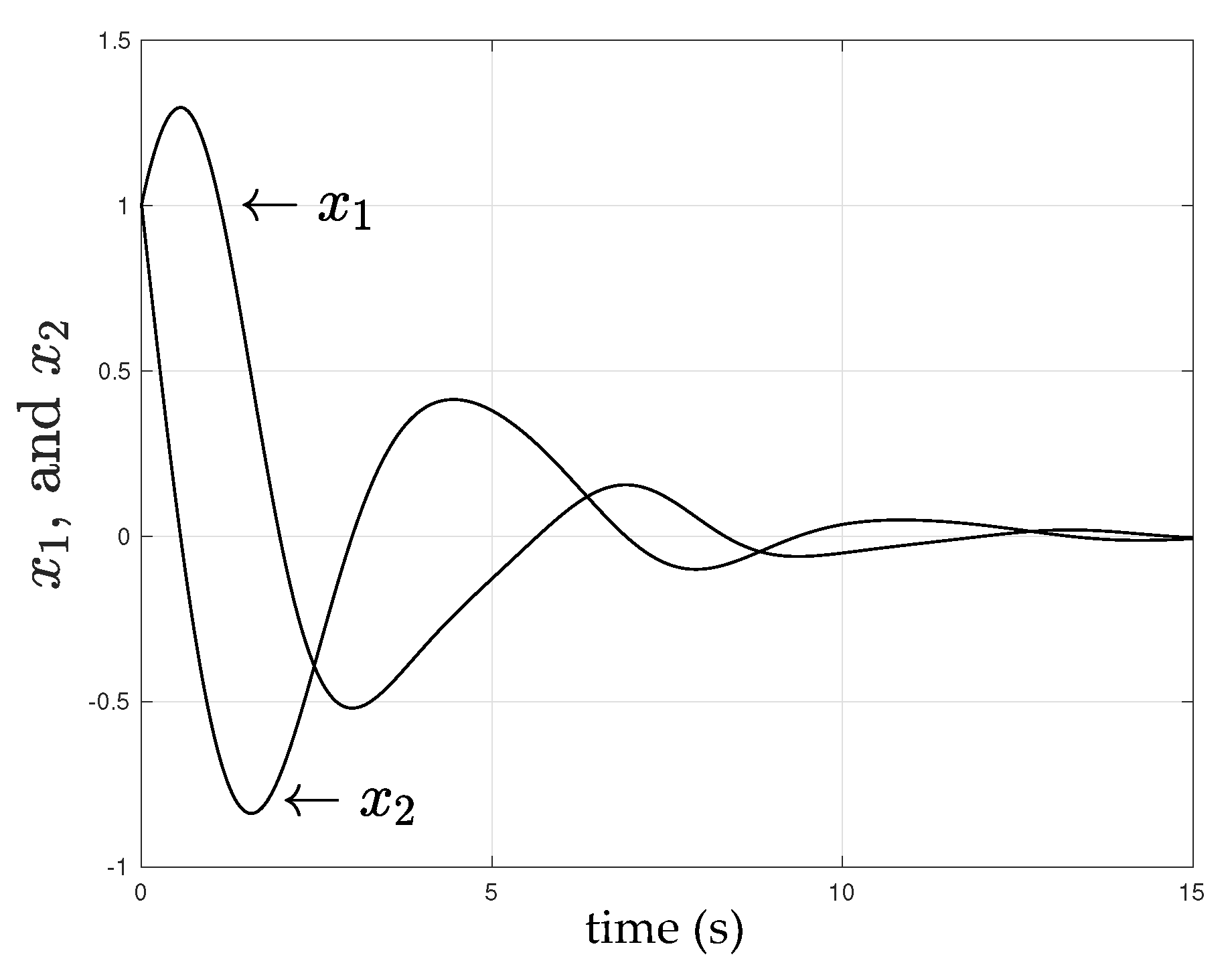
Solving the above LMIs, we have $K_1=[-0.2179,-1.7081]$, $K_2=[-0.2179,7.2919]$ for the regular PDC controller in (41). The control performance of the regular controller is shown in Figure 4, where the uncertainty is not considered, i.e., $F=0$, where the initial state is set to be $x_0={[1,1]}^T$. It is clear that the regular controller is able to stabilize the unstable system when the uncertainty is not considered.

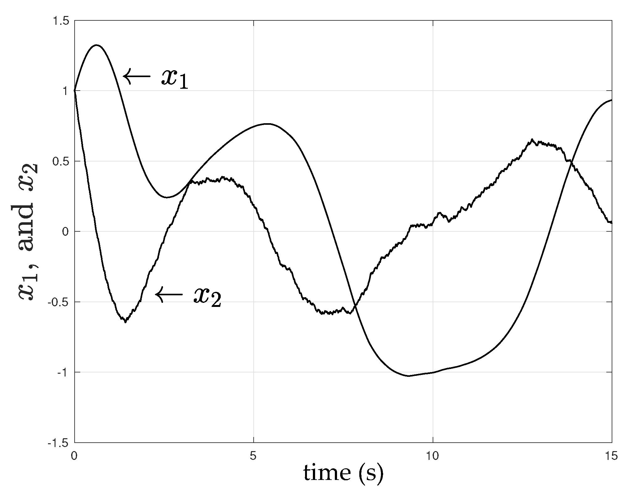
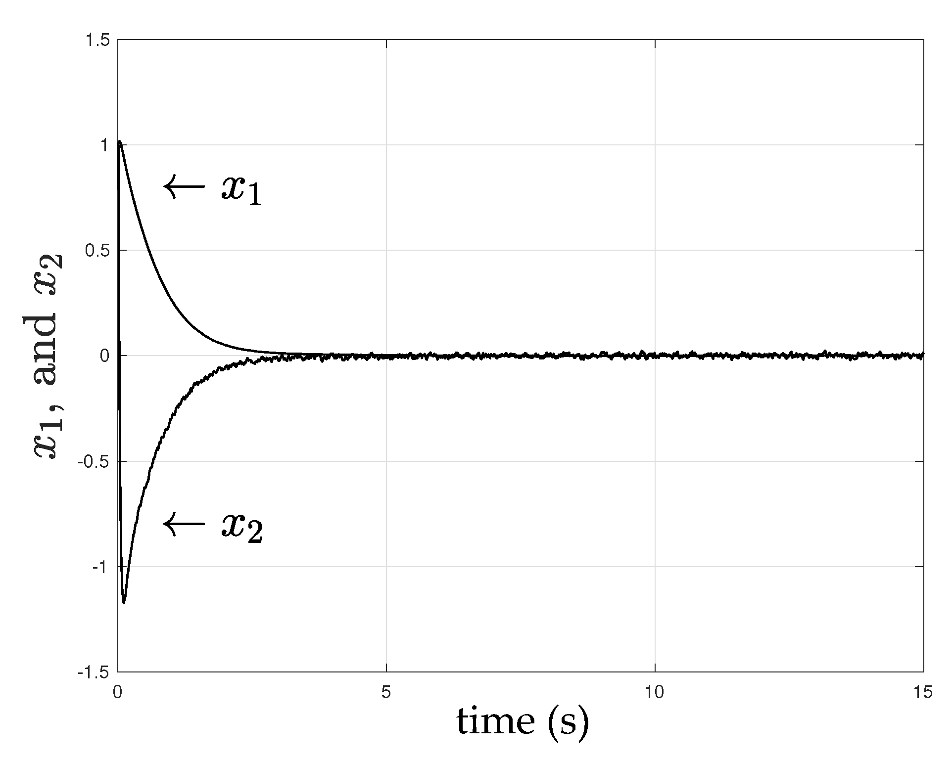
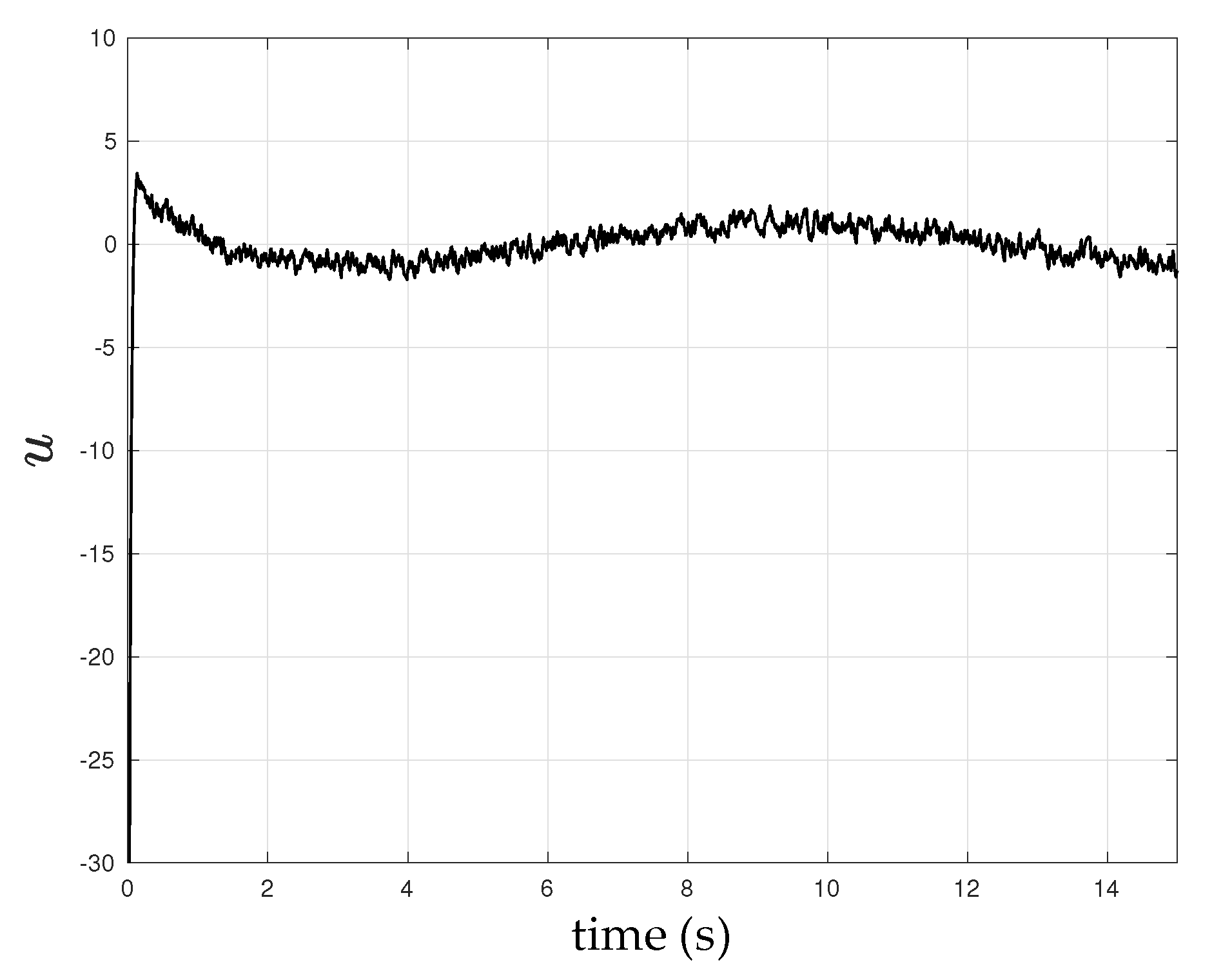
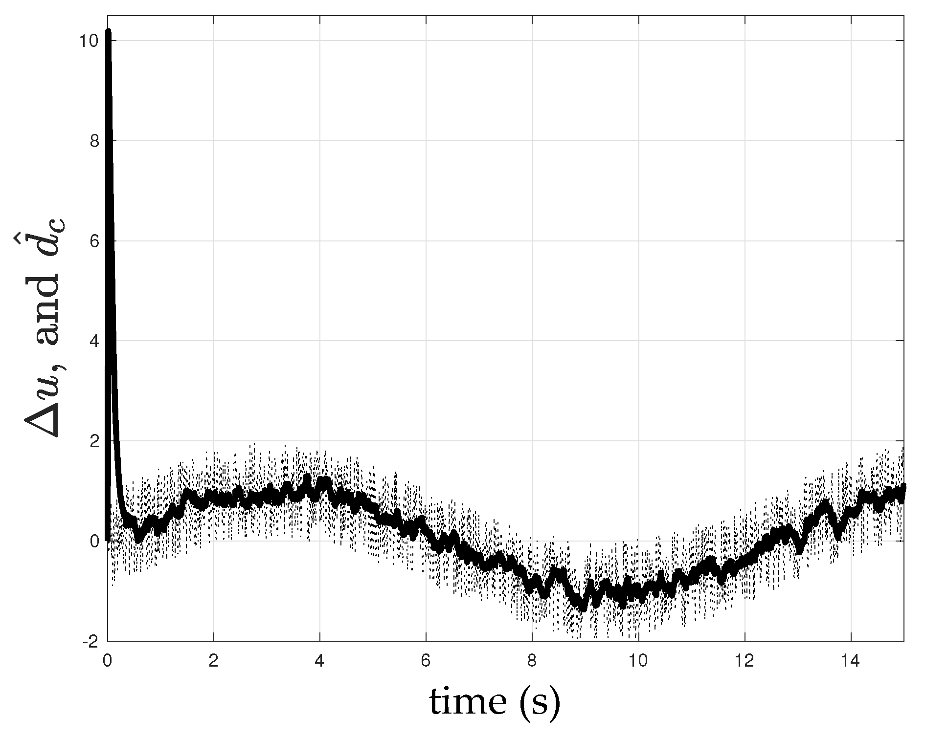
However, when the uncertainty in Figure 1 is applied to the system, as shown in Figure 5, the regular controller no longer stabilizes the system. On the contrary, with the uncertainty observer (A4), the proposed controller (15) can stabilize the system effectively under the same circumstances. Figure 6 and Figure 7 depict the behaviors of state and control input, respectively. At the same time, as shown in Figure 8, the observer (A4) is able to catch the trajectory (bold line) of the uncertainty $\Delta u$.

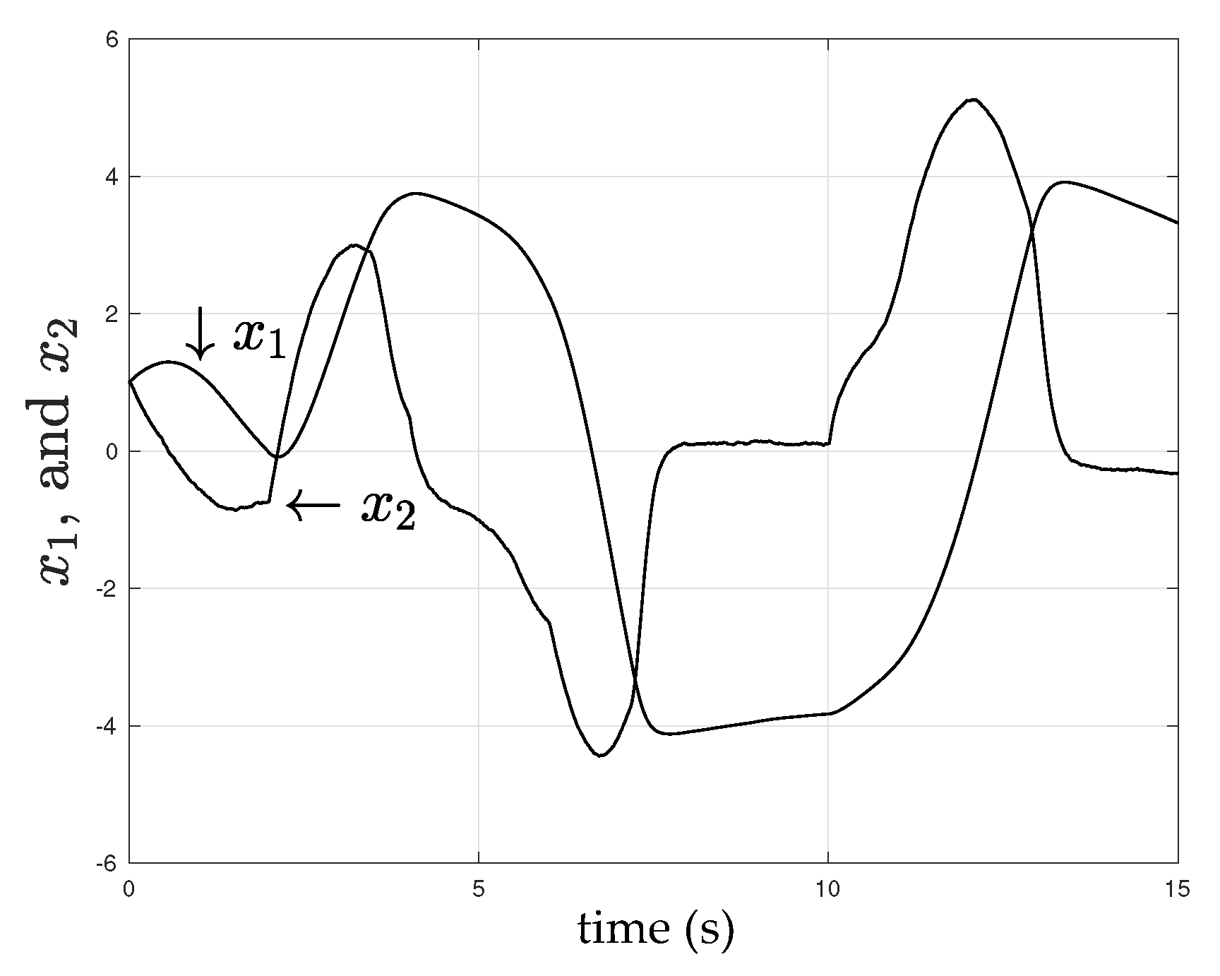
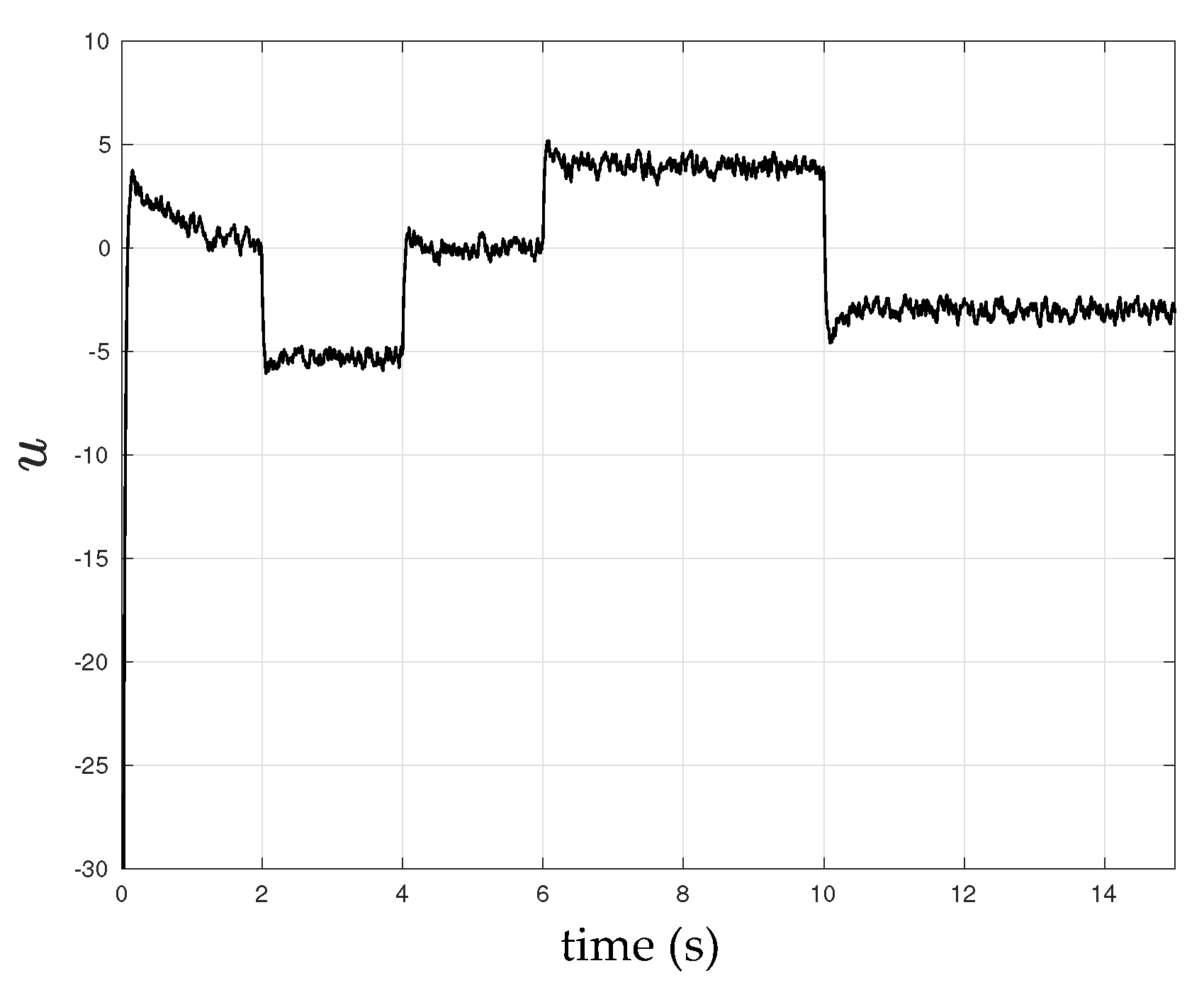
When it comes to the uncertainty in Figure 2, as shown in Figure 9, the regular controller (41) once again is unable to stabilize the system. However, the proposed controller is very effective at handling the same situation. The behaviors of the state and control input are depicted in Figure 10 and Figure 11, respectively, while the behavior of the uncertainty observer (A4) is depicted in Figure 12.

5. Conclusions

In order to improve the control performance when using the widely-used T-S fuzzy model to design a controller, a term called uncertainty was considered in the model. While the stability of the whole control system involving such uncertainty can be guaranteed by certain conditions such as LMIs, one of the main contributions in this paper was making an effort to employ some information of the uncertainty whenever possible in the controller design. Consequently, as verified in the Simulation Section, an observer that is able to catch the trajectory of partial uncertainty that shares the same control matrix as the control input was proposed without the often used condition that the uncertainty must be time independent. Compared to the regular PDC controller, simulation results showed that the controller proposed in this paper was more effective at handling the situation where the uncertainty appears. However, all the designs in this paper were developed on the condition that all of the state is available, which may restrain its applications to practical systems. As one of the ongoing challenges, we are working on an observer of the state along with the one related to the uncertainty for the controller design. It is apparent that the approach shown in this paper cannot be straightforwardly extended to the state-unknown case on account of the uncertainty. Finally, it is worth noting that, when the approach proposed in this paper is applied to a real-time system, the uncertainty may not cover all the discrepancy between the real system and its T-S fuzzy model. In this sense, the system stability margin and robustness should be considered when developing such approaches in future works.

References

- Takagi, T.; Sugeno, M. Fuzzy identification of systems and its applications to modeling and control. IEEE Trans. Syst. Man Cybern. 1985, 15, 116–132. [Google Scholar] [CrossRef]
- Khalil, H.K. Nonlinear Systems; Prentice Hall: Upper Saddle River, NJ, USA, 2002. [Google Scholar]
- Lin, C.; Wang, Q.; Lee, T. H∞ output tracking control for nonlinear systems via T-S fuzzy model approach. IEEE Trans. Syst. Man Cybern. Part B Cybern. 2006, 36, 450–457. [Google Scholar]
- Han, H. H∞ approach to T-S fuzzy controller for limiting reconstruction errors. Int. J. Syst. Sci. 2014, 45, 399–406. [Google Scholar] [CrossRef]
- Wei, Y.; Qiu, J.; Shi, P.; Lam, H.K. A new design of H∞ piecewise filtering for discrete-time nonlinear time-varying delay systems via T-S fuzzy affine models. IEEE Trans. Syst. Man Cybern. 2016, 36, 1–14. [Google Scholar] [CrossRef]
- Wei, X.; Wu, Z.; Karimi, H.R. Disturbance observer-based disturbance attenuation control for a class of stochastic systems. Automatica 2016, 63, 21–25. [Google Scholar] [CrossRef]
- Han, H.; Su, C.Y.; Stepanenko, Y. Adaptive control of a class of nonlinear systems with nonlinearly parameterized fuzzy approximators. IEEE Trans. Fuzzy Syst. 2001, 9, 315–323. [Google Scholar]
- Liu, Y.J.; Gao, Y.; Tong, S.; Li, Y. Fuzzy approximation-based adaptive backstepping optimal control for a class of nonlinear discrete-time systems with dead-zone. IEEE Trans. Fuzzy Syst. 2016, 24, 16–28. [Google Scholar] [CrossRef]
- Tian, Z.; Li, S.; Wang, Y. T-S fuzzy neural network predictive control for burning zone temperature in rotary kiln with improved hierarchical genetic algorithm. Int. J. Model. Identif. Control 2016, 25, 323–334. [Google Scholar]
- Wang, L.X.; Mendel, J.M. Fuzzy basis functions, universal approximation, and orthogonal least-squares learning. IEEE Trans. Neural Netw. 1992, 3, 807–813. [Google Scholar] [CrossRef] [PubMed]
- Cao, Y.Y.; Lin, Z. Robust stability analysis and fuzzy-scheduling control for nonlinear systems subject to actuator saturation. IEEE Trans. Fuzzy Syst. 2003, 11, 57–67. [Google Scholar]
- Chen, B.; Liu, X.; Tong, S.; Lin, C. Guaranteed cost control of T-S fuzzy systems with state and input delays. Fuzzy Sets Syst. 2007, 158, 2251–2267. [Google Scholar] [CrossRef]
- Zhang, F.; Wang, Q.G.; Lee, T.H. Adaptive and robust controller design for uncertain nonlinear systems via fuzzy modeling approach. IEEE Trans. Syst. Man Cybern. 2004, 34, 166–178. [Google Scholar] [CrossRef]
- Han, H. AAdaptive fuzzy controller for a class of uncertain nonlinear systems. J. Jpn. Soc. Fuzzy Theory Intell. Inform. 2009, 21, 577–586. [Google Scholar]
- Hou, M.; Muller, P.C. Design of observer for linear systems with unknown inputs. IEEE Trans. Autom. Control 1992, 37, 871–875. [Google Scholar] [CrossRef]
- Kalsi, K.; Lian, J.; Hui, S.; Zak, S.H. Slide-mode observer for systems with unknown inputs: A high-gain approach. Automatica 2010, 46, 347–353. [Google Scholar] [CrossRef]
- Liu, G.; Cao, Y.Y.; Chang, X.H. Fault detection observer design for fuzzy systems with local nonlinear models via fuzzy Lyapunov function. Int. J. Control Autom. Syst. 2017, 15, 2233–2242. [Google Scholar] [CrossRef]
- Yang, J.; Chen, W.H.; Li, S. Non-linear disturbance observer-based robust control for systems with mismatched disturbances/uncertainties. IET Control Theory Appl. 2011, 5, 2053–2062. [Google Scholar] [CrossRef] [Green Version]
- Yang, J.; Li, S.; Yu, X. Sliding-mode control for systems with mismatched uncertainties via a disturbance observer. IEEE Trans. Ind. Electron. 2013, 60, 160–169. [Google Scholar] [CrossRef]
- Han, H.; Higaki, Y. A design of polynomial fuzzy controller with disturbance observer. Proceedings of Joint 7th International Conference on Soft Computing and Intelligent Systems and 15th International Symposium on Advanced Intelligent Systems (SCIS & ISIS 2014), Kita-Kyushu, Japan, 3–6 December 2014. [Google Scholar]
- Han, H. An observer-based controller for a class of polynomial fuzzy systems with disturbance. IEEJ Trans. Electric. Electron. Eng. 2016, 11, 236–242. [Google Scholar] [CrossRef]
- Soffker, D.; Yu, T.J.; Muller, P. State estimation of dynamical systems with nonlinearities by using proportional-integral observer. Int. J. Syst. Sci. 1995, 26, 1571–1582. [Google Scholar] [CrossRef]
- Wu, D.; Han, H. Design of T-S fuzzy controller with disturbance observer. IEEJ Trans. Electric. Electron. Eng. 2016, 11, 198–205. [Google Scholar] [CrossRef]
- Wang, Y.; Xie, L.; Souza, C.D. Robust control of a class of uncertain nonlinear system. Syst. Control Lett. 1992, 19, 139–149. [Google Scholar] [CrossRef]
- Orlov, Y.; Aguilar, L.T.; Acho, L.; Ortiz, A. Asymptotic harmonic generator and its application to finite time orbital stabilization of a friction pendulum with experimental verification. Int. J. Control 2008, 81, 227–234. [Google Scholar] [CrossRef]
- Tanaka, K.; Wang, H. Fuzzy Control System Design and Analysis—A Linear Matrix Inequality Approach; Wiley: New York, NY, USA, 2001. [Google Scholar]
Figure 1.
Sinusoidally-perturbed uncertainty.
Figure 2.
Piecewise constantly-perturbed uncertainty.
Figure 3.
phase plane with and .
Figure 4.
Control performance of the regular parallel distributed compensation (PDC) controller (41) where in (38).
Figure 8.
in Figure 1 and its estimate (bold line).
Figure 12.
in Figure 2 and its estimate (bold line).
© 2018 by the authors. Licensee MDPI, Basel, Switzerland. This article is an open access article distributed under the terms and conditions of the Creative Commons Attribution (CC BY) license (http://creativecommons.org/licenses/by/4.0/).
Share and Cite
MDPI and ACS Style
Han, H.; Hamasaki, D. A Controller Design Based on Takagi-Sugeno Fuzzy Model Employing Trajectory of Partial Uncertainty. Designs 2018, 2, 7. https://doi.org/10.3390/designs2010007
AMA Style
Han H, Hamasaki D. A Controller Design Based on Takagi-Sugeno Fuzzy Model Employing Trajectory of Partial Uncertainty. Designs. 2018; 2(1):7. https://doi.org/10.3390/designs2010007
Chicago/Turabian StyleHan, Hugang, and Daisuke Hamasaki. 2018. "A Controller Design Based on Takagi-Sugeno Fuzzy Model Employing Trajectory of Partial Uncertainty" Designs 2, no. 1: 7. https://doi.org/10.3390/designs2010007