High-Resolution Surface Water Classifications of the Xingu River, Brazil, Pre and Post Operationalization of the Belo Monte Hydropower Complex


Abstract
:1. Summary
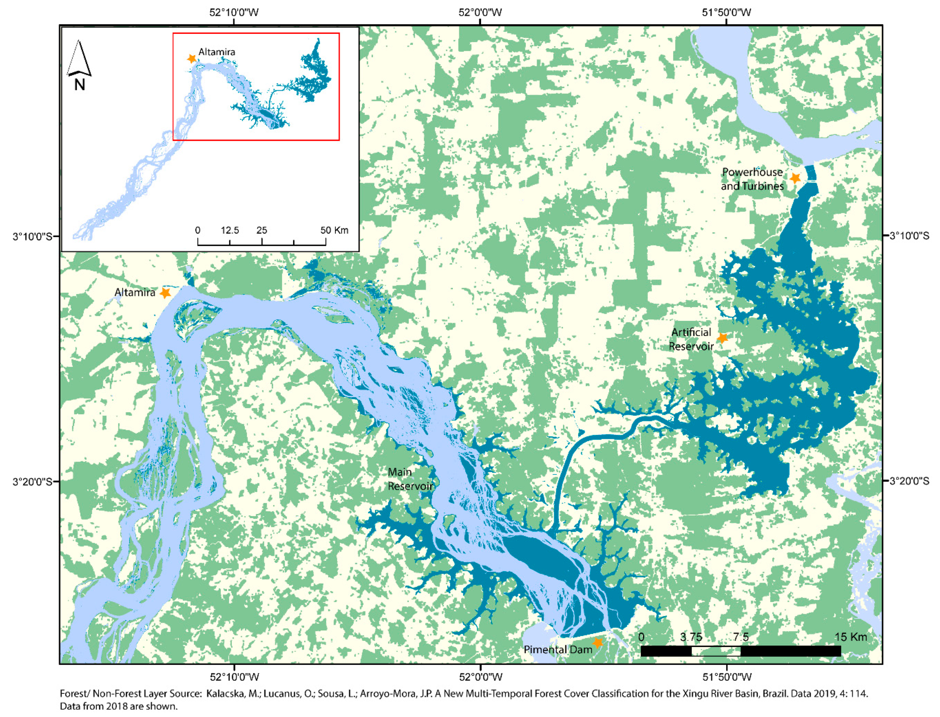
2. Data Description
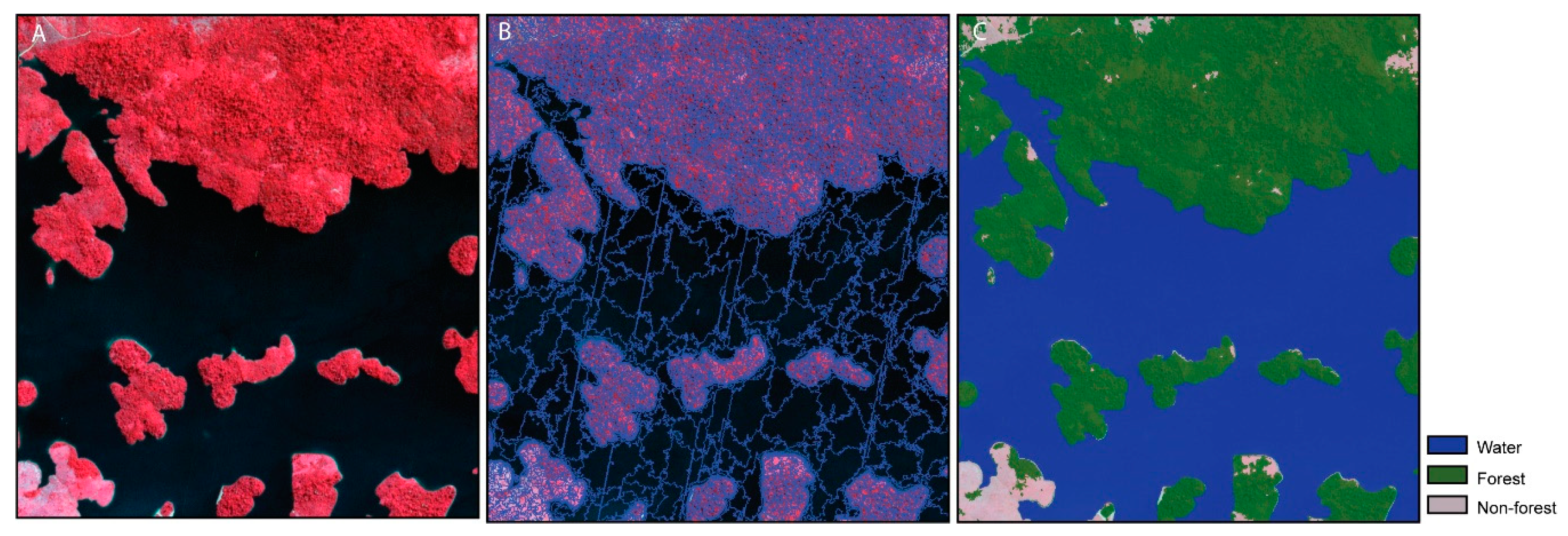
3. Methods
4. User Notes
Author Contributions
Funding
Conflicts of Interest
References
- Dagosta, F.C.P.; De Pinna, M. The fishes of the Amazon: Distribution and biogeographical patterns, with a comprehensive list of species. Bull. Am. Mus. Nat. Hist. 2019, 431, 1–163. [Google Scholar] [CrossRef] [Green Version]
- Camargo, M.; Giarrizzo, T.; Isaac, V. Review of the geographic distribution of fish fauna of the Xingu river basin. Ecotropica 2004, 10, 123–147. [Google Scholar]
- Jézéquel, C.; Tedesco, P.A.; Bigorne, R.; Maldonado-Ocampo, J.A.; Ortega, H.; Hidalgo, M.; Martens, K.; Torrente-Vilara, G.; Zuanon, J.; Acosta, A.; et al. A database of freshwater fish species of the Amazon Basin. Sci. Data 2020, 7, 96. [Google Scholar] [CrossRef] [PubMed] [Green Version]
- Bratman, E.; Dias, C.B. Development blind spots and environmental impact assessment: Tensions between policy, law and practice in Brazil’s Xingu river basin. Environ. Impact Assess. Rev. 2018, 70, 1–10. [Google Scholar] [CrossRef]
- Perez, M.S. Where the Xingu bends and will soon break. Am. Sci. 2015, 103, 395–397. [Google Scholar] [CrossRef]
- Latrubesse, E.M.; Arima, E.Y.; Dunne, T.; Park, E.; Baker, V.R.; d’Horta, F.M.; Wight, C.; Wittmann, F.; Zuanon, J.; Baker, P.A.; et al. Damming the rivers of the Amazon basin. Nature 2017, 546, 363–369. [Google Scholar] [CrossRef] [PubMed]
- Winemiller, K.O.; McIntyre, P.B.; Castello, L.; Fluet-Chouinard, E.; Giarrizzo, T.; Nam, S.; Baird, I.G.; Darwall, W.; Lujan, N.K.; Harrison, I.; et al. Balancing hydropower and biodiversity in the Amazon, Congo, and Mekong. Science 2016, 351, 128–129. [Google Scholar] [CrossRef] [PubMed] [Green Version]
- de Araújo, K.R.; Sawakuchi, H.O.; Bertassoli Jr, D.J.; Sawakuchi, A.O.; da Silva, K.D.; Vieira, T.B.; Ward, N.D.; Pereira, T.S. Carbon dioxide (CO2) concentrations and emission in the newly constructed Belo Monte hydropower complex in the Xingu River, Amazonia. Biogeosciences 2019, 16, 3527–3542. [Google Scholar] [CrossRef] [Green Version]
- Fearnside, P.M. Dams in the Amazon: Belo Monte and Brazil’s hydroelectric development of the Xingu River basin. Environ. Manag. 2006, 38, 16. [Google Scholar] [CrossRef] [PubMed]
- Fearnside, P.M. Greenhouse gases in the environmental impact study for the Belo Monte Hydroelectric Dam. Novos Cad. NAEA 2011, 14, 5–19. [Google Scholar]
- Fearnside, P.M. Belo Monte: Actors and arguments in the struggle over Brazil’s most controversial Amazonian dam. DIE ERDE J. Geogr. Soc. Berl. 2017, 148, 14–26. [Google Scholar] [CrossRef]
- Pekel, J.F.; Cottam, A.; Gorelick, N.; Belward, A.S. High-resolution mapping of global surface water and its long-term changes. Nature 2016, 540, 418–422. [Google Scholar] [CrossRef] [PubMed]
- MapBiomas Project. MapBiomas Project-Collection v3.1 of the Annual Land Use Land Cover Maps of Brazil. Available online: https://mapbiomas.org/en (accessed on 1 August 2019).
- Demarchi, L.; van de Bund, W.; Pistocchi, A. Object-based ensemble learning for pan-european riverscape units mapping based on copernicus VHR and EU-DEM data fusion. Remote Sens. 2020, 12, 1222. [Google Scholar] [CrossRef] [Green Version]
- Kalacska, M.; Arroyo-Mora, J.P.; Lucanus, O.; Sousa, L.; Pereira, T.; Vieira, T. Deciphering the many maps of the Xingu–an assessment of land cover classifications at multiple scales. bioRxiv 2019. [Google Scholar] [CrossRef]
- Chen, G.; Weng, Q.H.; Hay, G.J.; He, Y.N. Geographic object-based image analysis (GEOBIA): Emerging trends and future opportunities. Gisci. Remote Sens. 2018, 55, 159–182. [Google Scholar] [CrossRef]
- RapidEye, A.G. Satellite Imagery Product Specifications. Available online: https://www.planet.com/products/satellite-imagery/files/160625-RapidEye%20Image-Product-Specifications.pdf (accessed on 5 June 2020).
- Planet Team. Understanding PlanetScope Instruments. Available online: https://developers.planet.com/docs/data/sensors/ (accessed on 5 June 2020).
- Planet Team. Planet Imagery Product Specification: PlanetScope & RapidEye; Planet: San Francisco, CA, USA, 2016; Available online: https://www.planet.com/products/satellite-imagery/files/1610.06_Spec%20Sheet_Combined_Imagery_Product_Letter_ENGv1.pdf (accessed on 5 June 2020).
- Planet Team. Planet. Surface Reflectance v2.0; Planet: San Francisco, CA, USA. p. 18. Available online: https://assets.planet.com/marketing/PDF/Planet_Surface_Reflectance_Technical_White_Paper.pdf (accessed on 5 June 2020).
- Johansen, K.; Sohlbach, M.; Sullivan, B.; Stringer, S.; Peasley, D.; Phinn, S. Mapping banana plants from high spatial resolution orthophotos to facilitate plant health assessment. Remote Sens. 2014, 6, 8261–8286. [Google Scholar] [CrossRef] [Green Version]
- Ma, L.; Li, M.C.; Ma, X.X.; Cheng, L.; Du, P.J.; Liu, Y.X. A review of supervised object-based land-cover image classification. ISPRS J. Photogramm. Remote Sens. 2017, 130, 277–293. [Google Scholar] [CrossRef]
- Benz, U.C.; Hofmann, P.; Willhauck, G.; Lingenfelder, I.; Heynen, M. Multi-resolution, object-oriented fuzzy analysis of remote sensing data for GIS-ready information. ISPRS J. Photogramm. Remote Sens. 2004, 58, 239–258. [Google Scholar] [CrossRef]
- Silva, J.P.; Pereira, D.I.; Aguiar, A.M.; Rodrigues, C. Geodiversity assessment of the Xingu drainage basin. J. Maps 2013, 9, 254–262. [Google Scholar] [CrossRef] [Green Version]
- Barbosa, T.A.P.; Rosa, D.C.O.; Soares, B.E.; Costa, C.H.A.; Esposito, M.C.; Montag, L.F.A. Effect of flood pulses on the trophic ecology of four piscivorous fishes from the eastern Amazon. J. Fish Biol. 2018, 93, 30–39. [Google Scholar] [CrossRef] [PubMed]


| Date (DD-MM-YY) | Scene ID | Satellite |
|---|---|---|
| 04-07-11 | 2237610 | RE2 |
| 04-07-11 | 2237609 | RE2 |
| 04-07-11 | 2237509 | RE2 |
| 04-07-11 | 2237510 | RE2 |
| 04-07-11 | 2237508 | RE2 |
| 04-07-11 | 2237410 | RE2 |
| 04-07-11 | 2237408 | RE2 |
| 04-07-11 | 2237409 | RE2 |
| 04-07-11 | 2237307 | RE2 |
| 04-07-11 | 2237308 | RE2 |
| Date (DD-MM-YY) | Scene ID | Satellite | Sector |
|---|---|---|---|
| 24-07-19 | 132529 | 101f | Artificial reservoir |
| 24-07-19 | 132530 | 101f | Artificial reservoir |
| 24-07-19 | 132531 | 101f | Artificial reservoir |
| 24-07-19 | 132532 | 101f | Artificial reservoir |
| 11-08-19 | 130512 | 1020 | Iriri to Pimental |
| 11-08-19 | 130514 | 1020 | Iriri to Pimental |
| 11-08-19 | 130515 | 1020 | Iriri to Pimental |
| 11-08-19 | 130516 | 1020 | Iriri to Pimental |
| 11-08-19 | 130517 | 1020 | Iriri to Pimental |
| 11-08-19 | 132859 | 1006 | Iriri to Pimental |
| 11-08-19 | 132900 | 1006 | Iriri to Pimental |
| 13-08-19 | 143914 | 53-106a 1 | Iriri to Pimental |
| 24-08-19 | 130314 | 104e | Iriri to Pimental |
| 24-08-19 | 130315 | 104e | Iriri to Pimental |
| 24-08-19 | 130316 | 104e | Iriri to Pimental |
| 24-08-19 | 130317 | 104e | Iriri to Pimental |
| 24-08-19 | 130318 | 104e | Iriri to Pimental |
| 24-08-19 | 130632 | 1020 | Iriri to Pimental |
| 24-08-19 | 132930 | 0f17 | Iriri to Pimental |
| 24-08-19 | 132931 | 0f17 | Iriri to Pimental |
| 24-08-19 | 132932 | 0f17 | Iriri to Pimental |
| 24-08-19 | 132933 | 0f17 | Iriri to Pimental |
| 24-08-19 | 132934 | 0f17 | Iriri to Pimental |
| 11-07-19 | 132719 2 | 1032 | Artificial reservoir |
| Water-Reference | Land-Reference | User’s Accuracy (%) | |
|---|---|---|---|
| Water-Classification | 654 | 45 | 93.6 |
| Land-Classification | 4 | 840 | 99.5 |
| Producer’s Accuracy (%) | 99.4 | 94.9 | OA = 96.8 |
| Water-Reference | Land-Reference | User’s Accuracy (%) | |
|---|---|---|---|
| Water-Classification | 748 | 1 | 99.9 |
| Land-Classification | 2 | 812 | 99.8 |
| Producer’s Accuracy (%) | 99.7 | 99.9 | OA = 99.8 |
© 2020 by the authors. Licensee MDPI, Basel, Switzerland. This article is an open access article distributed under the terms and conditions of the Creative Commons Attribution (CC BY) license (http://creativecommons.org/licenses/by/4.0/).
Share and Cite
Kalacska, M.; Lucanus, O.; Sousa, L.; Arroyo-Mora, J.P. High-Resolution Surface Water Classifications of the Xingu River, Brazil, Pre and Post Operationalization of the Belo Monte Hydropower Complex. Data 2020, 5, 75. https://doi.org/10.3390/data5030075
Kalacska M, Lucanus O, Sousa L, Arroyo-Mora JP. High-Resolution Surface Water Classifications of the Xingu River, Brazil, Pre and Post Operationalization of the Belo Monte Hydropower Complex. Data. 2020; 5(3):75. https://doi.org/10.3390/data5030075
Chicago/Turabian StyleKalacska, Margaret, Oliver Lucanus, Leandro Sousa, and J. Pablo Arroyo-Mora. 2020. "High-Resolution Surface Water Classifications of the Xingu River, Brazil, Pre and Post Operationalization of the Belo Monte Hydropower Complex" Data 5, no. 3: 75. https://doi.org/10.3390/data5030075