

Bioenergetic Model of the Highly Exploited Shark Mustelus schmitti under a Global Warming Context

1
Department of Biology, Biochemistry and Pharmacy, National South University (Departamento de Biología, Bioquímica y Farmacia–UNS), Bahía Blanca 8000, Argentina
2
National Institute of Fisheries Science, Busan 46083, Republic of Korea
3
National Institute of Fisheries Research and Development (Instituto Nacional de Investigación y Desarrollo Pesquero), Mar del Plata 7602, Argentina
4
Faculty of Fisheries Sciences, Hokkaido University, Hakodate 040-8567, Japan
*
Author to whom correspondence should be addressed.
Diversity 2023, 15(11), 1118; https://doi.org/10.3390/d15111118
Submission received: 15 September 2023
/
Revised: 25 October 2023
/
Accepted: 25 October 2023
/
Published: 27 October 2023
(This article belongs to the Special Issue Biology and Ecology of Sharks and Their Relatives: New Insights for a Correct Management and Conservation)
Abstract
:Bioenergetic models are tools that allow the evaluation of the effect of environmental variables on fish growth. Successful implementation of this approach has been achieved in a few elasmobranch species. Our objective was to develop a bioenergetic model for Mustelus schmitti. The model developed showed a good fit to the field data available and accurately described the growth of this species. The practical example developed in this study provides novel population estimates of prey consumption and daily ration for the species. Results also indicate that this species would be susceptible to the effects of climate change. In the simulated climate change scenarios, the energy budget of M. schmitti was significantly altered, with increased food consumption and impaired growth. While there exists a number of limitations for the model developed in this article, namely its limitation to immature individuals, and its restricted temperature model, it provides an important tool for the management of this and other shark populations under heavy exploitation.
1. Introduction
The conservation of elasmobranches is currently a priority for the resource management plans of several countries (e.g., Mediterranean countries, the USA, Canada, and Australia [1]). Many elasmobranch species constitute major fisheries resources, providing food and income for people worldwide [2]. While it is true that fishing, by-catch, and habitat destruction are the major threats for most elasmobranches, the fate of elasmobranches is even more uncertain under the current scenario of climate change [3,4,5]. The shifts in the abiotic conditions, a product of climate change, are expected to produce severe impacts on marine organisms and consequently originate socioeconomic disruptions according to the Intergovernmental Panel on Climate Change [6,7]. Predicting how fish growth can be affected by external environmental factors has, therefore, become a priority in fisheries management [5].
The development of bioenergetic models provides a potentially powerful approach for predicting how changes in environmental variables can impact on fish individual growth, which can then be extrapolated to population levels [8,9,10]. Bioenergetic models are mathematical tools that are used to predict the growth, reproduction, and survival of fish in different environmental conditions. These models are based on the principles of bioenergetics, which is the study of how organisms acquire and use energy. In fisheries assessment, bioenergetic models are used to estimate the amount of food that a fish needs to consume in order to maintain its body weight and grow [8,10,11]. The models take into account factors such as the metabolic rate, the water temperature, the food availability, and the size and age structure of the species. Successful implementation of such an approach has so far been performed only on a handful of elasmobranch species (for example, [8]). A recent review has only found ten studies dealing with the bioenergetics of elasmobranches, and only four developing bioenergetics models [10].
A bioenergetics model describes the use of energy of an organism, and how it is distributed between the main metabolic processes. Depending on the specifics of the base model employed, it has seven main processes: growth, respiration, consumption, reproduction, specific dynamic action, excretion, and egestion. Being a mechanistic model, one of the processes can be estimated if the rest are known [12,13]. If, for example, the consumption rate is known, bioenergetics models can be used to predict growth and/or reproduction, both of which are crucial for survival at both the individual and population levels. The most common way an animal increases its energetic demand is via elevated respiration, which mostly proxies activity levels [14,15]. The standard metabolic rate (SMR), a main component of the respiration process can also be affected by changes in water temperature. In ectotherms, SMR increases approximately exponentially when temperature increases [16]. Active metabolic rate sometimes equated to routine metabolic rate (RMR; see [16] for a full treatment of terminology of metabolic rates) can be increased during migrations, predator/prey interactions, mating behavior, tides, temperature, or human disturbances (e.g., [15,17,18]). To supply an increased metabolic demand, an animal can either increase its food consumption or use the energy from growth or reproduction [8,9].
It should be clear now that in order to simulate these processes, bioenergetics models require a wealth of information, not only on the biology of species being studied but also on the abiotic characteristics of the environment in which the target species inhabits, as well as on other biological components of the ecosystem. Such an abundance of information is available only on a handful of species, many of which are not elasmobranches [7]. In the vast majority of bioenergetics studies, the estimates needed to develop a functional model are taken from the literature, from ecologically or taxonomically close species [19]. A few exceptions are those studies that conduct the experimental or field assessments necessary to feed the model-specific estimates (for example, [8]).
Traditionally, bioenergetics models have been employed on planktonic bony fish species, which have short lifespans and relatively simple behaviors and are usually the target of industrial fishing and subjected to strong management plans [19,20,21]. These species are generally abundant and ecologically and taxonomically uniform, which makes borrowing data from other similar species less error-prone. That is not the case for elasmobranches, which are mostly demersal and have long lifespans and complex mating and young-rearing behaviors [22]. Additionally, they are taxonomically and ecologically much more diverse [23], making data borrowing much more error-prone. Luckily, some species are quite abundant and subjected to continuous exploitation, which, to some extent, makes them the target of scientific inquiry. One such species is the triakid Mustelus schmitti. The genus Mustelus is an important cosmopolitan group of sharks with broad distribution across the continental shelves of several countries [24]. This species is a small-sized demersal coastal shark [24], it is viviparous and forms sexual aggregations near nursery areas [25]. It feeds mainly on benthic prey, primarily crustaceans and polychaeta worms, but larger individuals also prey on benthic fish. It itself is prey to other larger sharks that inhabit its distribution areas, such as Notorynchus cepedianus, Carcharhinus brachyurus, Carcharias taurus, and Sphyrna tiburo. It is extensively exploited by commercial and artisanal fisheries along its distribution [24,26] and represents one of the most landed sharks in the coastal waters of the Southwestern Atlantic Ocean [27]. In fact, continued fishing intensity and population decline trends over the last decades have led the International Union for Conservation of Nature (IUCN) Red List of Threatened Species to categorize this species as critically endangered [28]. Additionally, the habitat of this shark encompasses one of the most intensely studied marine areas of Argentina, El Rincon (38–42° S, <50 m depth). This area, covering approximately 45,000 km2, is the main fishing ground for the industrial fleets targeting this shark [29]. The literature on M. schmitti from the authors of this article alone covers reproduction, trophic ecology, age and growth, and metabolic dynamics [26,30,31,32,33,34], and provides most of the needed information to develop a bioenergetics model based on species-specific estimates. In addition, many other articles on M. schmitti have been published, which together provide a deep understanding of these and other biological and ecological aspects of this shark [25,27,35,36,37,38,39,40,41]. All this information provides an abundance of scientific literature, that makes this species an ideal first candidate for modeling.
This approach provides a holistic and multifaceted understanding of the intricate interplay between biological, ecological, and physiological aspects, which is pivotal for informed and sustainable exploitation of aquatic resources [7,42]. The integration of these diverse data sources into a bioenergetics modeling framework is particularly powerful because it enables the quantification of energy flow within the ecosystem [43]. In a science-based fisheries management context, this comprehensive framework empowers decision-makers with the ability to optimize fishing quotas and practices, aligning them with the species’ ecological role, life history, and physiological requirements. It also aids in forecasting the potential consequences of different management scenarios, such as harvest restrictions or habitat conservation measures, on both the target species and the broader ecosystem [7,44].
The aim of this research was to develop a bioenergetics model for M. schmitti and apply it as an assessment tool for proper conservation and fisheries management of this elasmobranch. With that aim, we developed algorithms using both traditionally obtained fisheries statistics data and experimental data, allowing us to provide a tool that can be adapted to other highly exploited elasmobranchs worldwide. We employed the extensive biological databases compiled by our team, comprising biological parameters of the species, population dynamics, trophic ecology, respirometry data, and age and growth data. Finally, we applied the model to simulate the fate of an M. schmitti population under two predicted global warming scenarios.
2. Materials and Methods
2.1. Bioenergetics Model
The bioenergetics fish model we used in this work is a modification and adaptation of the one developed by Rudstam [45], Ware [46], Beauchamp et al. [47], Trudel et al. [48] and Kamezawa et al. [49], who modified it for chum salmon [12]. We incorporated other parametrizations [8] and adjusted this model to better incorporate the particular biological and physiological features of a demersal shark. The bioenergetics model developed was used to predict the daily survival, daily body weight, and food consumption of 3000 sexless individuals over a maximum age of 7 years. This species is known to reach sexual maturity approximately at that age, so we modeled juvenile individuals to leave reproduction costs aside [32]. Predictions were summarized as the average weight and length, food consumed, and the amount of energy needed by an average individual each year.
The parameter values used as input in the model were specified based on research and experimental results (most of them published in [15,26,30,31,33,34,50,51,52]) or from literature-reported results on closely related species. The individual processes and parameters are described below.
2.1.1. Growth
The growth rate (dW/dt, gshark × d−1) of an individual (non-reproductive) M. schmitti was calculated as weight increment per unit of weight (W, gshark) per time:
where C is consumption, E is excretion, F is egestion or losses due to feces, R is respiration or losses through metabolism, and S is specific dynamic action or losses due to energy costs of digesting food. All rates except the caloric conversion rate between prey and shark (CALp/CALs, unitless) are in the units of grams prey/gram shark/day (gprey × gshark−1 × d−1).
dW/dt = (C − (R + S + F + E)) × (CALp/CALs) × W
M. schmitti caloric density was set to be 1294 cal × gshark−1, based on calorimetric determinations (Molina, unpublished data); 1100 and 991 cal/gprey−1 was used for the prey, either polychaetes or crabs [30].
2.1.2. Consumption
Realized consumption (C) was estimated as the proportion of the maximum daily ration for an individual at a particular mass and temperature [11,12]. This consumption is also affected by the rate at which the species can digest food and able to consume more prey, which also depends on temperature [53]. The consumption function used in the model is taken from Kishi et al. [12]:
where Cmax = maximum specific consumption rate in gprey × gshark−1 × d−1, the values of which were determined from Molina and Lopez Cazorla [30], p = prey—the specific proportion of Cmax, determined from a modeled projection of M. schmitti diet for each day of the year (see below for details), f(T) = temperature-dependence function for consumption, T = water temperature in °C, DR = digestion rate, expressed as a proportion. ac is the intercept of the mass-dependence function for a 1 gshark at the optimum water temperature, bc is the coefficient of the mass dependence, and W = wet weight in g.
C = Cmax × p × f(T) × DR
Cmax = ac × Wbc
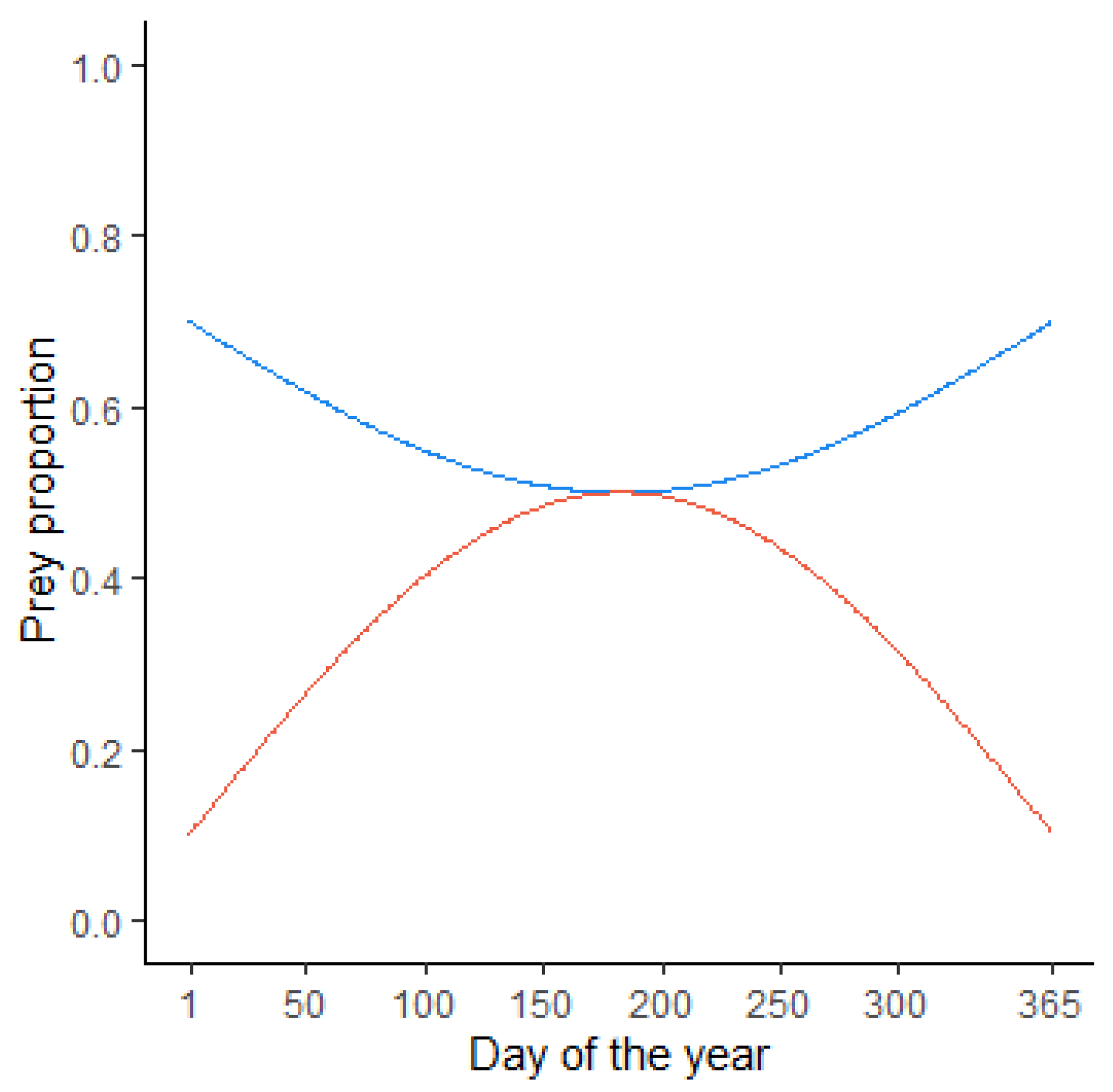
Considering the flexibility of the M. schmitti diet, research from Anegada Bay was used to rebuild a “generalized” diet. The Prey-Specific Index of Relative Importance (PSIRI) [54] was used as the criteria to identify the two most important prey items. Polychaetes and crabs were found to be the dominant prey and made up this generalized diet. For modelling simplicity, it was considered that the food available for M. schmitti was geographically stable and the same regardless of age, despite studies documenting regional and ontogenetic variations in its composition [30,37]. The seasonal change in the PSIRI was used to build a model of the daily proportional contribution of each prey to the diet of the sharks (Figure 1).
Digestion rates for chondrichthyans have seldom been studied (e.g., [55]); therefore, we have taken the analytical approach outlined in the seminal work of He and Wurtsbaugh [53] who provide an empirical model of gastric evacuation rates for fish in general. This parameter is expressed as the times per day the fish can empty its stomach, which depends on temperature by the following exponential equation [53]:
where 24 represents the number of hours in a day, and the rest of the equation is the hourly digestion rate, where di and dc are the empirical intercepts and proportionality constant, and T is the water temperature in °C.
DR = 24 × (di × exp(dc×T))
Estimates for ac and bc were determined using available information on stomach repletion and egestion times [31]. The estimates produced are well within the ranges previously estimated for other species of elasmobranches [8,56]. We use the temperature dependence function found in Thornton and Lessem [57] that has been shown to effectively describe the relationship of temperature with the proportion of Cmax available to the shark and can graphically be represented as the product of two sigmoid curves (similar to a Q10 relationship) [8]. The shape of the curve is governed by xk1–4 and te1–4 parameters [12,49], which we estimated from sea bottom temperature models for the El Rincon area [51] and trophic ecology data [30,31,37].
2.1.3. Respiration
The respiration rate is the amount of energy used for routine metabolism and it depends on body weight, water temperature, and activity rate:
where ar is the intercept of the allometric mass function (gprey × gshark−1 × d−1), br is the slope of the allometric mass function (unitless), g(T) is Q10 temperature correction function (modified from 8) for standard metabolic rate, and ACT represents the proportional increase in metabolic expenditure from standard to routine metabolic rate (i.e., active metabolism). The value 0.5 represents the proportion of time the individual is in each metabolic state each day (resting vs. active). Q10 = temperature sensitivity, T = temperature experienced by the shark (°C), and Tref = reference temperature that corresponds to the values of ar and br. 2.94 is a conversion factor from g O2 × gshark −1 × d−1 from into gprey × gshark −1 × d−1 [13].
R = ar × Wbr × g(T) × 0.5 + ar × Wbr × g(T) × ACT × 0.5 × 2.94
g(T) = Q10(T−Tref)/10
ACT = 1 + ((RMR − SMR)/SMR)
2.2. Temperature
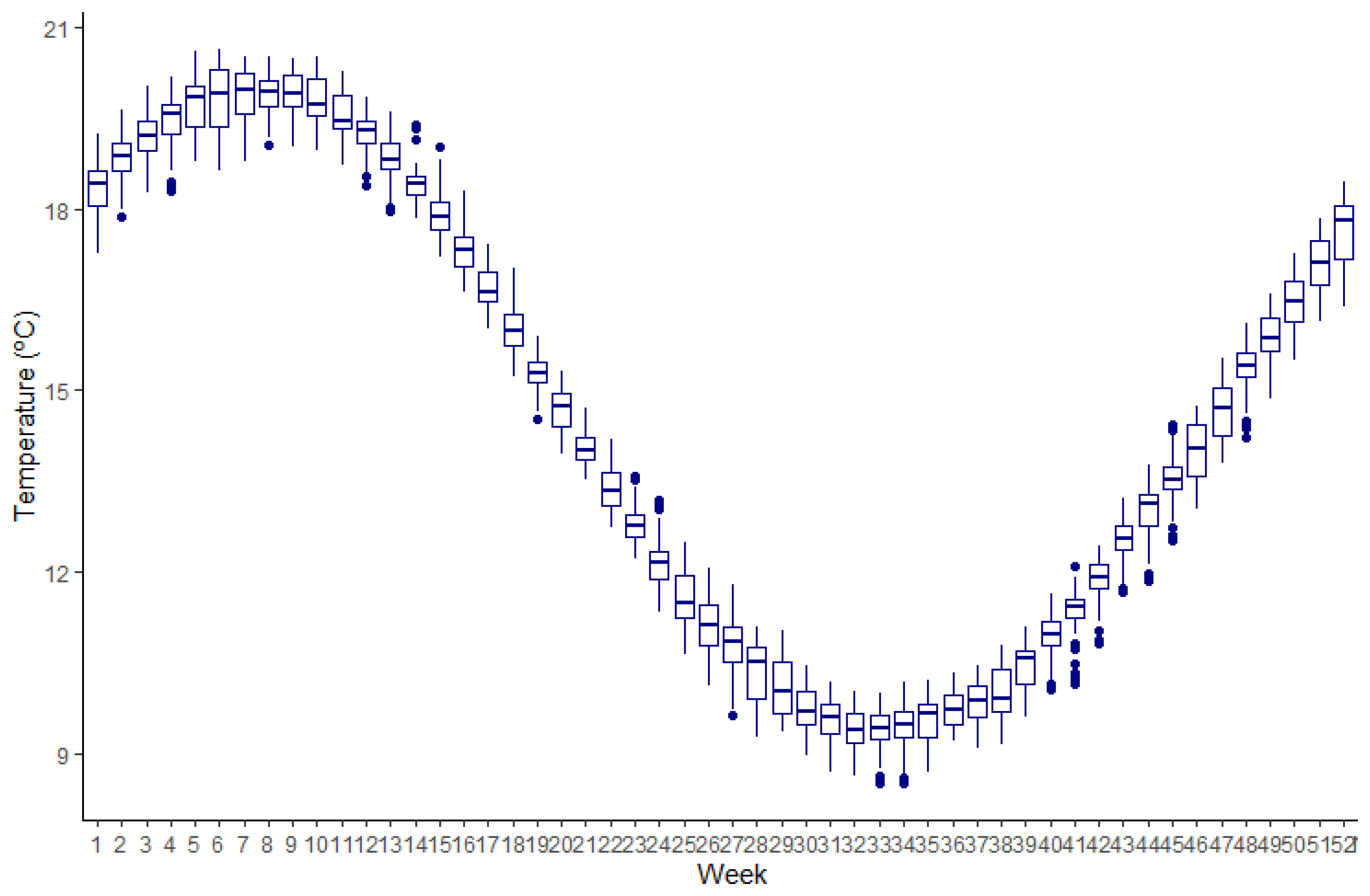
A daily temperature function, starting on the 1 January and ending on the 31 December, was developed using a continuous data series of daily bottom temperature for the El Rincón coastal area between 1980 and 2016, modeled by Elisio et al. [51]. This last study modeled daily temperature for the different depth ranges over the area. The daily bottom temperature considered in the present study was the average condition over the region for the 2000–2008 period (modeled period in the present study). It must be noted that the El Rincón coastal area corresponds to the locations where the biological data used to develop and calibrate the model were collected. The function generated a historical average water temperature for each day of the year in the models (Figure 2) which was fed to the various functions requiring a temperature input.
2.3. Model Uncertainties, Simulated Variability, and Monte Carlo Methods
Unlike other models that employ fixed parameters, we opted for the use of sampling distributions for several point estimates (sensu [8,9,59]). These probability distributions were defined based on either assumptions about the distributions of input variables (from recommendations in [8,9,59]) or driven by the distributions observed in the data of M. schmitti compiled by the authors. The possible sampling distributions were (1) normal distributions, used for variables that are symmetrical around the mean (i.e., T, initial W, constants for S, E, and F); (2) log-normal distributions, used for right-skewed variables with a lower limit of zero and no upper bound (i.e., SMR, RMR, intercepts); and (3) uniform distributions, used for variables with an upper and lower limit, where sampling probabilities are constant between the limits (i.e., prey proportions).
2.3.1. Individual-Level Variability
Several sources of individual variability in the growth of M. schmitti were simulated: initial weight, weight-specific consumption and respiration intercepts, and egestion, excretion, and specific dynamic action constants. To emulate differences in growth efficiency, variability in the ar and ac parameters was incorporated by assigning each individual the normally distributed mean and standard deviation estimates (from the experimental data) to a log-normal distribution. Similarly, initial weight, S, E, and F were incorporated in the model as estimates from a normal distribution. These sources of variation were programmed to vary for each individual and remain constant for the entirety of each individual’s simulation.
2.3.2. Environmental-Level Variability
We incorporated two sources of environmental variability, daily temperature and prey availability. For each day of the simulation, each individual was assigned a daily water temperature from a normal distribution with the mean equal to the average temperature predicted by the temperature model and a standard deviation of 1 °C. These variations would emulate both daily spatial oscillations in the bottom temperature as well as temperatures unpredicted by the temperature model. The proportion of Cmax for polychaetes and crabs available for each day was provided by the previously described model based on PSRI and was fed to a uniform distribution, with a and b estimated as the model output +/−20%. These variations in prey availability seek to emulate the patched distribution of prey along the feeding areas of the sharks. These two sources of variability were programmed to change each day, as opposed to the individual variability sources, which were different for each individual for the entire simulation.
2.3.3. Monte Carlo Simulations
Model estimates of growth were run 3000 times, each representing an individual M. schmitti being born on 1 January. To ensure realistic initial sizes, initial W was based on observed weight-at-birth information [26,31,59,60]. A mean and standard deviation (SD) of weight-at-birth was estimated and fed to a normal distribution, which provided values for each individual. The model stopped on the 31 December of the seventh year, with a total of 2921 days modeled per individual shark, resulting in 8,763,000 model outcomes. From the raw data produced, centralization and variability statistics were derived and computed.
All model parameters are summarized in Table 1.
2.4. High Temperature Scenarios
We ran two scenarios, a baseline using current simulated bottom water temperatures [51] and two high water temperature scenarios. The high-temperature simulations examined the effect of a daily temperature change of +2 and +4 on the predicted growth of individuals, based on “moderate” and “severe” general ocean warming scenarios predicted for the year 2100 according to the IPCC 2022 report [6]. In these scenarios, we assumed that the foraging behavior would remain unchanged in response to the increased water temperatures and that the dynamics of prey abundance would also remain unchanged. To assess the effect of these scenarios on consumption, assuming growth is stable (i.e., as per the von Bertalanffy growth model), we fitted our bioenergetics model to estimate consumption and input weights generated by the von Bertalanffy growth model (taken from [32]). With these estimates, predicted weight-at-age, length-at-age, consumption-at-age, and respiration-at-age between scenarios were compared by fitting non-linear least square models to each scenario and then comparing them using a traditional significance test. Growth in weight was converted to total length by reversing the following equation [31]:
where W is the total weight in g, and TL is the total length in cm. The value 2.95 is the allometric coefficient of the length-weight relationship [31].
W = 4.287 × 10−06TL2.950
2.5. Practical Application
To showcase how the bioenergetic model can be applied in real-life scenarios, we conducted an estimation of the annual prey biomass consumption for stocks of M. schmitti in Anegada Bay. The abundance of the stock was determined based on the best available estimates from previous stock assessments for the area in front of the bay and further north in the common fishing ground of Argentina and Uruguay [24,61,62,63]. Although the age distribution of M. schmitti is expected to vary over time and across different locations, for our calculations, we made the assumption that the age class distribution of this stock resembled that of the age study performed within Anegada Bay by Molina and collaborators [32]. The bay comprises an area of 1550 km2 with many different areas and islands. We considered this total area as homogeneous for extrapolating the abundance obtained from averaging the estimates found in the bibliography [24,61,62,63]. This total abundance was partitioned by the proportions of each age group and then divided by the mean weight-at-age to obtain an estimate of the number of individuals. Finally, this estimate was multiplied by the amount of prey consumed per shark per age class to obtain the estimated prey consumption of the stock per age class. Daily ration was estimated following Bethea et al. [64] as the percentage of body weight ingested per day.
2.6. Statistical Analysis
The computational work, programming, and scripts were created in an R (R version 4.2.2) environment (R core team, [65]). For this task, we employed a series of additional packages, as well as for the development of graphics and other materials. These are ‘ggplot2′, ‘rvest’, ‘lattice’, ‘stringr’, ‘nlstools’, ‘FSA’, ‘lme4′, ‘car’, ‘MASS’, and ‘bbmle’. The model scripts used are available in Supplementary Materials.
3. Results
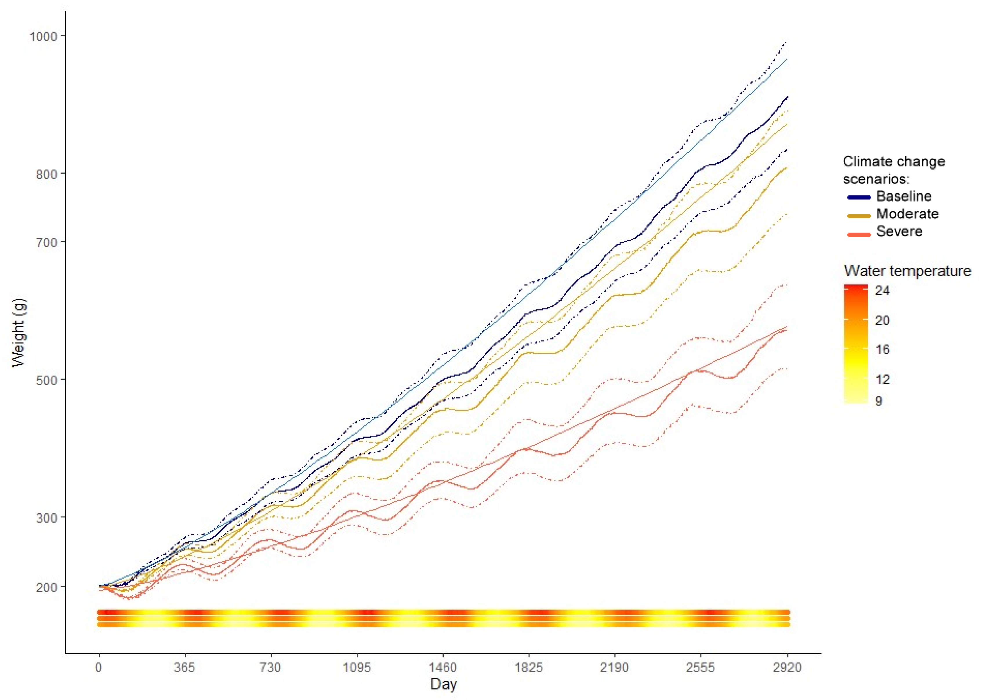
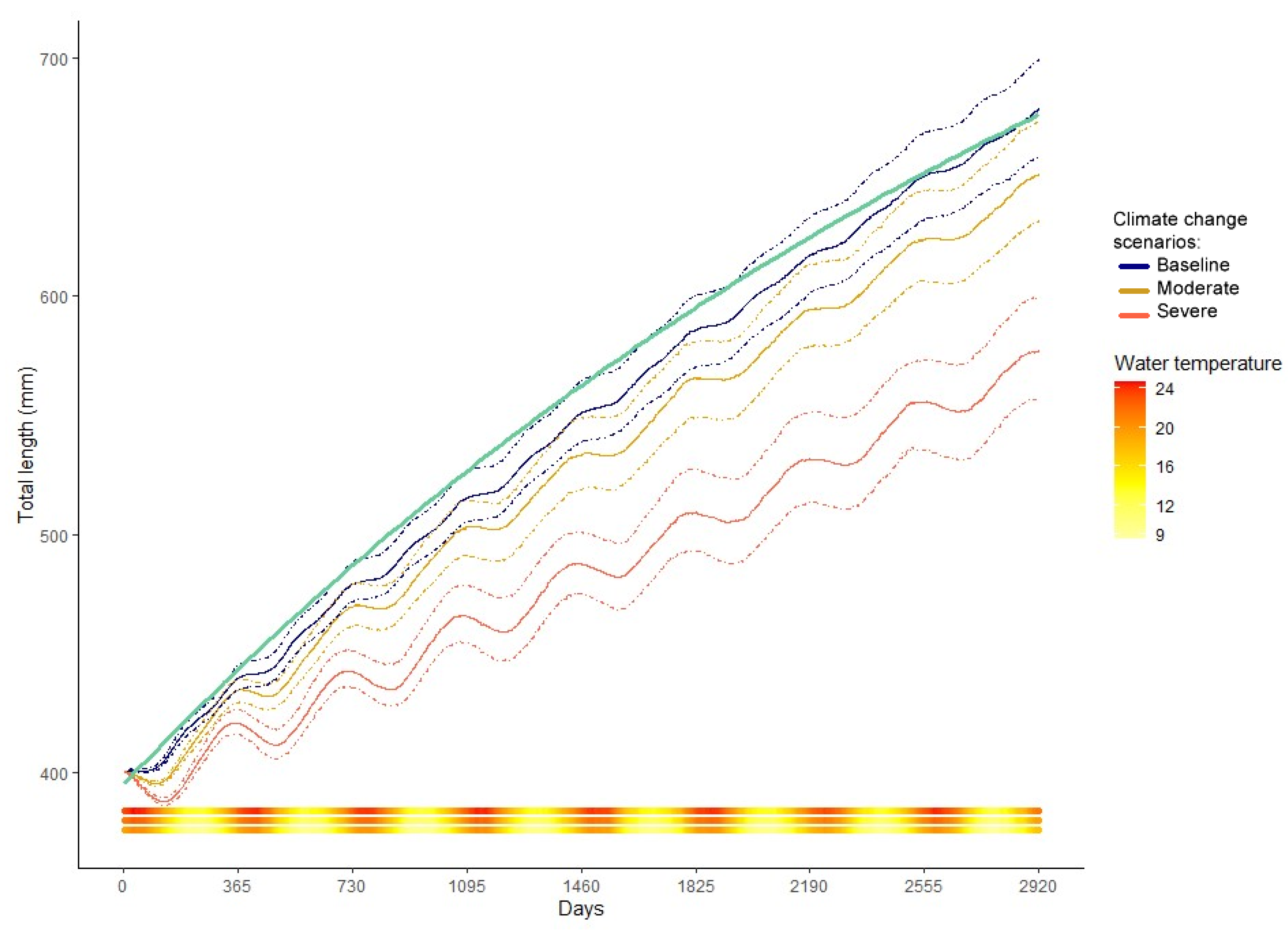
The baseline model-predicted median weights-at-age closely matched the von Bertalanffy growth model derived from observed size-at-age field data (Figure 3). There is, however, an important dispersion in the data simulated by the model (≅18%), as a product of the sampling distributions used on the point estimates. The simulated growth reached an average of 846 g (n = 3000) for the seventh year of life. Growth rates increased from 0.6 gshark × d−1 for year 0+ fish to 2.36 gshark × d−1 for seven-year-old (y.o.) fish. When the growth is observed as total length, as converted with the equation provided in Section 2.5, M. schmitti reaches 65 cm by the end of their 7th year of life. In their first two years of life, the juveniles grow approximately 5 cm per year, slowing down to 3 cm between their 6th and 7th year (Figure 4). The growth curve is in turn derived from the interaction of consumption and respiration. The interaction between these two components defines an effective growth season from the beginning of autumn, with a slight depression in winter, to early summer. The growth rate then diminishes greatly until next autumn (Figure 3).
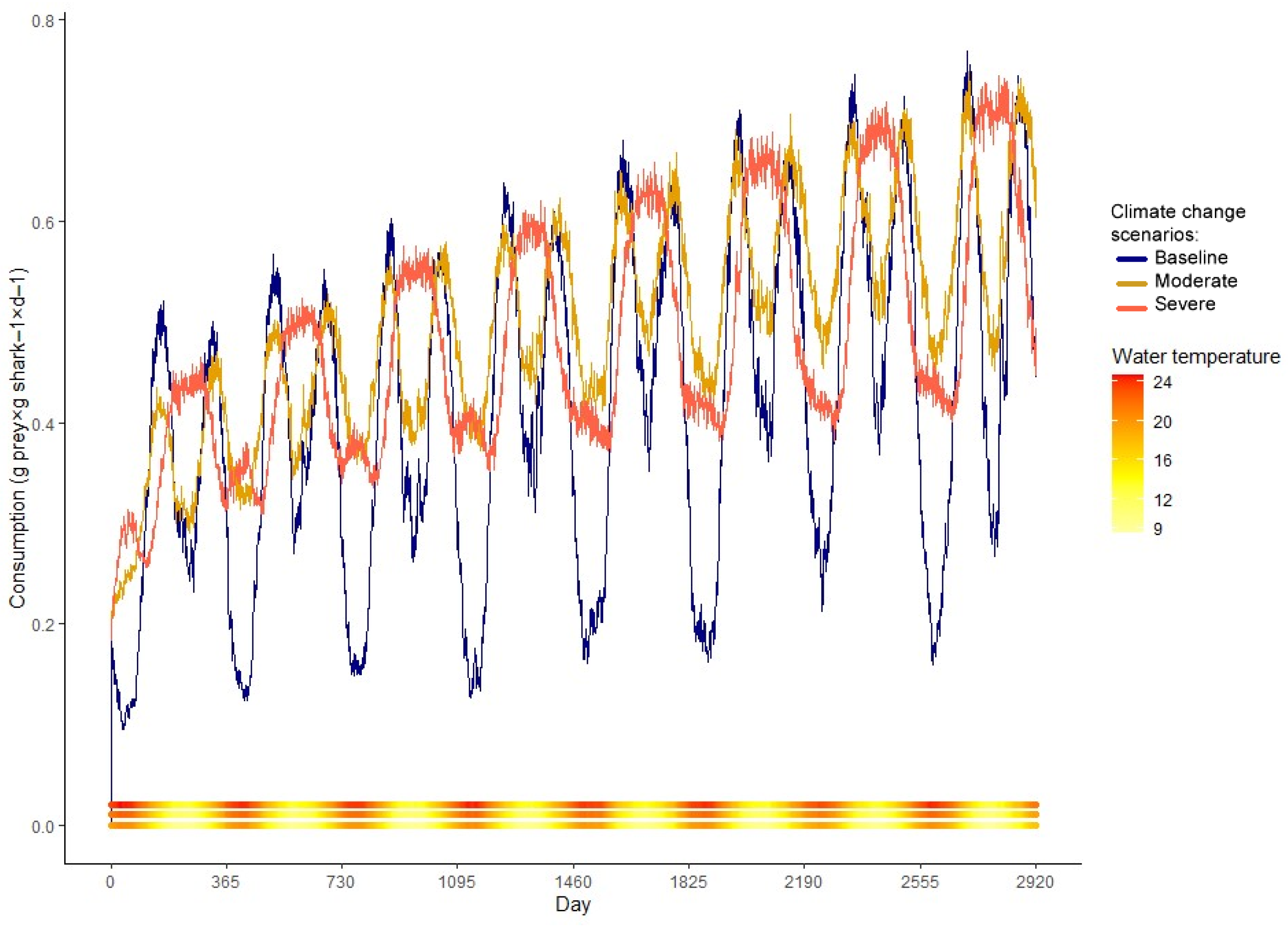
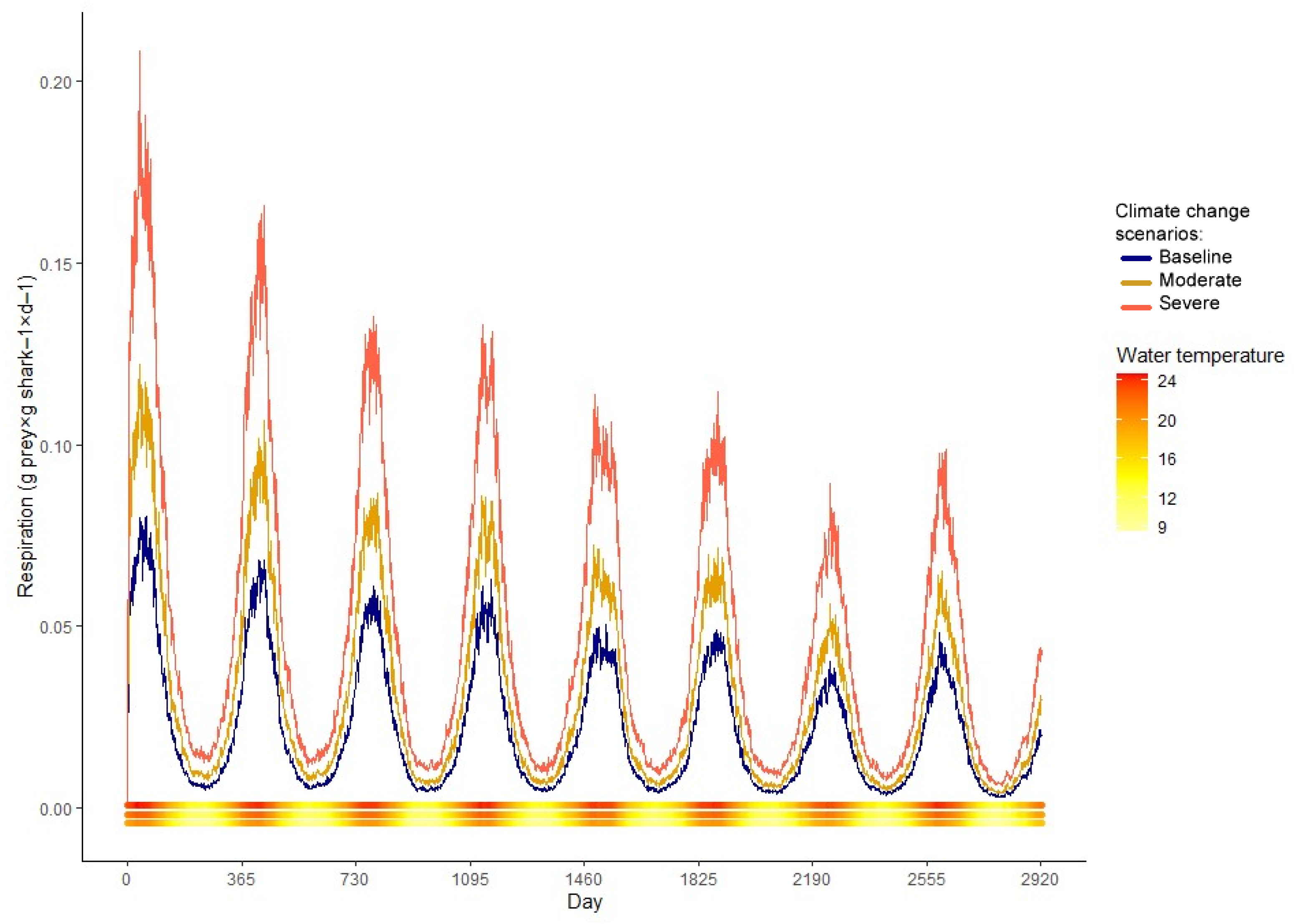
Consumption showed a yearly bimodal behavior with peaks in the seasons with intermediate temperatures and two drops, one more pronounced during summer and the other less during winter (Figure 5). It increased almost twofold from 0+ fish to 7 y.o. fish, from 0.35 to 0.52 gprey × gshark−1 × d−1, respectively. Respiration costs followed water temperature closely. It reaches a maximum in summer and a minimum in winter (Figure 6).
In the previous figures [3,4,5,6], the effects of increased temperatures for the two climate change scenarios, moderate (+2 °C), and severe (+4 °C) on the modeled variables can be observed. An increase in water temperature produced an increase in energy expenditure for the individuals, preventing them from reaching the baseline growth, especially in the severe scenario (Figure 3). If weights are converted to total length via the length-weight relationship (Figure 4), the individuals in the warmer simulations are also unable to attain baseline total length. For the moderate warming scenario, the reduction in age-specific average weights was between 5.6 and 18.1% compared to the baseline; the overall average decrease in weight-at-age (averaged over all ages) was 13.8%.
This reduction intensifies under severe warming conditions, with age-specific average weights between 10.3 and 46.4% smaller, and an overall average decrease of 34.6% (Table 2). The simulated climate change scenarios greatly affected estimated consumption as well. In the moderate scenario, the behavior of the consumption model remained the same, but the summer consumption depression is no longer bigger than the winter depression, to compensate for the higher cost of respiration and activity at higher temperatures (Figure 5). In the severe scenario, the behavior of the consumption model is altered; the winter depression disappears, showing a yearly unimodal pattern (Figure 5). The moderate scenario presented a 13.73% average yearly increase in consumption, while the severe showed an 18.29% increase in comparison with the baseline (Table 3). Respiration was also affected by the increase in temperature in the simulations. Under severe warming, younger individuals showed increased respiration expenditure in comparison to their older counterparts. This ontogenetic difference is not as notable for the moderate scenario nor the baseline model (Figure 6, Table 4).
Annual energy requirements were between 2500 (age +0) and 5000 (aye 7) Kcal under baseline conditions for an average shark to sustain continuous growth. In the moderate scenario, an average M. schmitti individual would have to procure an average of 8 cal per gram of body weight per day to sustain baseline growth. Sharks under the severe scenario would have to procure 20 cal per gram of body weight. The greater percentile difference was registered for +0 age in the severe scenario, where the need for energy doubles (Table 4). Total prey biomass consumption per shark was between 30 and 160 kg throughout the years modeled. If growth is held stable (i.e., as per the von Bertalanffy growth model), consumption increases by 11.5% on average in the moderate scenario and 19.4% in the severe scenario. This means an increase of 14.1 kg and 18.5 kg on average in prey biomass consumption per shark for the moderate and severe scenarios (Table 2).
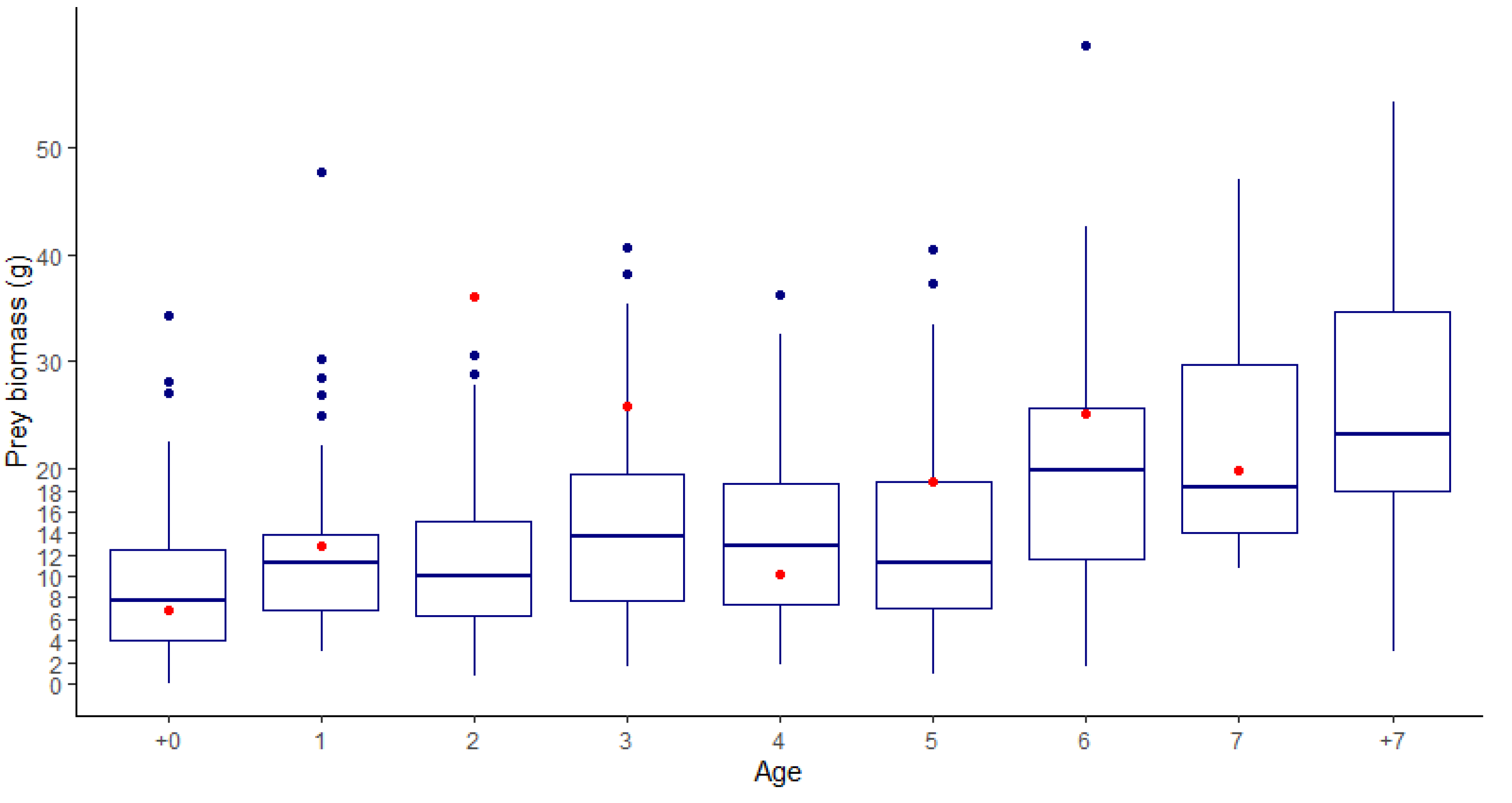
The results obtained for the practical example of the application of the model are outlined in Table 5. In total, the stock up to 7 y.o. sharks in Anegada Bay would consume a yearly 1,260,900.2 t of prey, between polychaetes and crabs. Prey consumption follows age-specific abundances, with age 1 individuals consuming the most, and age 7 the least. Daily rations were on average 4.58% for baseline, 5.25% for moderate, and 5.50% for severe scenarios. The daily ration estimated using these data can be converted to daily grams of prey consumption per shark, which mostly falls within the ranges of field observations of weight-specific average stomach content weights (Figure 7, except predictions for ages 2 and 3).
4. Discussion
4.1. The Bioenergetic Model
In this article, the bioenergetics of Mustelus schmitti were incorporated into a model that accurately predicted its growth, food consumption, and energy demands [30,32,37,58]. The focus was on this particular species due to its extensive research history, the wide distribution of the family Triakidae, and its protagonism in many of the most productive fisheries of elasmobranches worldwide [66,67,68,69,70]. In that sense, the model for this species could serve as a surrogate for understanding the relationship between disturbance, energy expenditure, and feeding opportunities in other shark species [71,72,73,74], particularly for those belonging to the widely distributed family Triakidae.
The main contribution of this study is the bioenergetic model per se, which allows for quantitative comparisons across different model variations and age groups, different environmental conditions, prey abundances, prey types, activity levels, etc. [75,76]. Model predictions for growth closely follow the mean sizes (both in weight and length) from field-sampled individuals [32,37]. Prey consumption estimated as size-specific daily prey biomass consumption also falls within the expected ranges for the species (Figure 7). Considering that these variables are well within the range of real parameters, predictions made about energy requirements and extrapolated prey biomasses needed are also likely to be accurate [77,78,79,80]. In this regard, the model provides an estimate not only of the food required for a population of M. schmitti to thrive but also an estimate of the standing abundance of the invertebrates that this species preys upon.
Another contribution of this study pertains to its practical example: the Anegada Bay conditions. Although these estimates can be improved by incorporating population-specific information, these preliminary assessments provide a quantitative framework for understanding how this population interacts with the environment [23,81]. The area used in the practical example has an important ecological value as it holds greatly biodiverse communities, owing to a high environmental complexity, composed of diverse aquatic environments such as wide muddy intertidal zones, sandy bottom beds, sand and gravel beaches, islands [26,82], and more recently, Magallana gigas reefs [83]. The refuge offered within the waters of this bay makes it an ideal nursery area [84] for many fish species, most of which are important, highly exploited, fisheries resources, among which M. schmitti stands out [30,31,32,50,85].
What was previously described should make clear that adequate management of fishery activities and conservation of the biodiversity of Anegada Bay should be a high priority [84] for the local government, a task in which the model developed in this article could be used effectively. Applying this bioenergetic model to other shark populations, with appropriate adjustments for species-specific parameters, could provide valuable comparative data. Such comparative studies could help identify population-specific vulnerabilities, assess the impacts of human activities, and design tailored conservation and management strategies for different shark populations [69,74].
An additional contribution of this work is that it provides estimates on the relationship of these sharks with their environment and their impact on ecosystem productivity and benthic species. While our estimates might seem rather high (more than a million tons of benthic prey), when converted to the total daily ration, it would represent an average of 4.6% of their body weight (Table 5), which is not only consistent with the field observations made by Molina and Lopez Cazorla [30] on site (Figure 7) but also similar (if even lower) for what was found for other shark species (see [64]). Improving upon these models would allow for better risk assessments associated with trophic transfer, uptake rates, and exposure to biotoxins or persistent contaminants through prey consumption [79,85,86,87].
4.2. Climate Change Scenarios
Bioenergetic models for fish are particularly relevant in the context of climate change, as they can help predict how changes in environmental conditions such as water temperature, and food availability may impact fish populations [88,89]. Climate change is expected to have significant impacts on fish populations, as rising temperatures are likely to alter the distribution and abundance of prey species [88,90,91,92]. In turn, changes in food availability may further affect growth, reproduction, and survivability [75,93,94].
In this work, the bioenergetics model developed for M. schmitti allowed for predictions on the potential effects of climate change on the energy budgets of the species. As expected, a warmer water temperature increased the energy requirements of M. schmitti, leading to an increase in food consumption. However, if food is restricted and does not keep pace with the increased demand, the model predicted notable reductions in growth, as would be reasonable to expect according to current research [95]. The amount of prey consumed by this species in our practical example is also notable. The prediction of younger individuals foraging for much more prey biomass than older juveniles highlights the importance of nursery areas for sharks, as the high productivity of these environments is needed to sustain the rapid growth these animals need [96,97].
In the water warming scenarios, this consumption is increased between 14% and 20%, depending on the scenario, which would imply higher predation pressure for the benthic communities that sustain these and other species [31,85,98,99]. Daily rations estimated for the baseline parameters are within reasonable ranges [64], and warmer conditions do not seem to impact these estimates too much; however, scaling these estimates according to fish biomass greatly increases the prey biomass needed by each cohort (Table 5).
M. schmitti possesses a wide distribution, from the south of Brazil to the Argentinian Patagonia, with wide variations in temperature across its range. It is fished throughout its distribution, being a main component of the landings of Argentina, Brazil, and Uruguay commercial fishing fleets [31,100]. Climate change is expected to have significant impacts on fisheries resources, with potential consequences for both the fishing industry and the ecosystems that support it [88,89,101,102]. One of the primary ways that climate change is expected to affect fisheries resources is through changes in ocean temperatures. As sea surface temperatures rise, the distribution and abundance of fish species may shift, potentially altering the composition of fisheries resources in the region [102,103,104]. The model predicts a drastic increase in consumption to maintain active growth or a marked decrease in growth if consumption needs cannot be satisfied in the climate change scenarios explored in this article. This situation may lead to changes in distribution for M. schmitti, with individuals migrating to more favorable latitudes or depths in favor of lower water temperatures [105] or change in fitness of different populations or even local extinctions [94,102,106,107].
Aside from the direct impacts of increasing ocean temperatures on M. schmitti populations, the distribution and abundance of various species that serve as the prey of M. schmitti may also be affected by potential factors such as time-lagged abiotic conditions on a finer temporal scale. In some cases, marine processes are better explained by time-lagged ecological variables, such as sea surface temperature rather than simultaneous values [108]. Ocean temperatures are often considered to have an accumulation period prior to being reflected in higher trophic levels through ocean food chains [109,110]. While, as we have discussed above, the impacts of climate change on fisheries resources are complex and multifaceted, providing even limited tools for predicting its effects could prove useful to mitigate these impacts [7,89,102,111].
4.3. Model Limitations
There are two main limitations to the model developed in this article. First, bioenergetic models are based on simplifying assumptions about the physiology and behavior of fish species. While these assumptions are based on empirical data, they may not accurately capture the complexity of real-world conditions, which can vary greatly depending on the species, life stage, size structure-specific mortality rates, complex behaviors, and species-species interactions, and may therefore limit their accuracy [74,76,112,113,114,115]. Particularly hot or cold years could change the estimations in this model, as could behavioral shifts in response to changing salinity, which may affect food conversion or prey selection [56,72,84,97,112]. Predation risk and competition can all influence the behavior and energy requirements of fish but were not fully accounted for in this model [116,117]. It would be expected that predation avoidance involves increased activity, perhaps not contemplated in our activity parameter [116]. Competition may result in reduced consumption when another species outcompetes M. schmitti in resource allocation [117]. As a consequence of these interactions, mortality rates are not usually constant among the different size ranges of a species. As a rule of thumb, it is higher in smaller fish, and as the individuals become larger, the mortality rate diminishes.
The factors described in the previous paragraph are too complex, and too little is known from field observations to incorporate into the model we developed with an acceptable level of certainty. Second, the model assumes a constant relationship between temperature and metabolic rate, which may not hold under all conditions [78,91]. While these gaps in our understanding impose limitations on the extrapolation of the predictions made in this study, they also point out several avenues for future research that can enhance the model’s accuracy and applicability. These include the following aspects:
- (1)
- Refinement and calibration: Further refinement of the bioenergetic model can be achieved by incorporating more precise and species-specific parameters [8,118]. Conducting controlled experimental studies to measure the energy consumption of M. schmitti, and determining the metabolizable energy of prey species would contribute to reducing uncertainties and improving model predictions [66,74,77]. Calibration of the model using independent field sampling data would also enhance its accuracy [115].
- (2)
- Incorporation of ecological factors: The model can be expanded to consider additional ecological factors that influence the energy requirements and behavior of M. schmitti [74,114]. Factors such as predation risk, competition, and habitat preferences can significantly impact the energy dynamics of the species [116,117]. Incorporating these factors, when sufficient data become available, would improve the model’s ecological realism and predictive power.
- (3)
- Long-term monitoring and data collection: Long-term monitoring of M. schmitti populations, including growth rates, prey availability, and environmental conditions, would provide valuable data for validating and updating the model [115,119]. Continued data collection efforts, such as tagging studies and dietary analyses, can contribute to a better understanding of the species’ energy requirements and feeding ecology [120].
This work incorporates many biological parameters estimated specifically in this species, which improved its accuracy when compared to other attempts at modeling bioenergetics on other species, which borrow most parameters from taxonomically distant species. In our work, a handful of parameters were indeed borrowed from close species, such as M. antarcticus and others, which incorporate unknown uncertainties in the model estimates. Despite that, the inclusion of Monte Carlo techniques and sampling distributions for point estimates permitted a certain level of variability to be incorporated into the model [8,9,66].
Despite these limitations, this and other bioenergetic models remain valuable tools for understanding the energy requirements and behavior of fish species [8,9,74,88]. By accounting for factors such as food availability, temperature, and predation risk, these models can provide important insights into the ecology and conservation of fish populations [7,102] and can inform management decisions aimed at promoting sustainable fisheries and protecting vulnerable species, such as M. schmitti.
5. Conclusions
The bioenergetic model developed for Mustelus schmitti in this study provides insights into the energy requirements and growth dynamics of this species. The model predicts the effects of climate change on the energy budgets of M. schmitti and highlights the potential impacts of warming water temperatures on food consumption and growth. Continued research and refinement of the model, along with long-term monitoring efforts, will enhance its accuracy and applicability, ultimately contributing to the science-based management of this important marine resource. Future research should focus on incorporating older age classes of the species, including the distinction between males and females. Adding a reproduction cost parameter to the model would provide a powerful enhancement to the model’s capabilities. Also, being able to add more complexity to the algorithms of trophic ecology would further refine the model. While in its current state, the model has limitations, it still serves as a valuable tool for understanding the bioenergetics of shark species and can contribute to the management and conservation of elasmobranch populations in the face of environmental change. Testing and applying this model in other locations will ensure a continued trial and error calibration of the model, which will surely change it from its current state into an improved version that would better reflect the complexity and nuances of the life history of this shark.
Supplementary Materials
The following supporting information can be downloaded at: https://www.mdpi.com/article/10.3390/d15111118/s1.
Author Contributions
Conceptualization, J.M.M., S.Y. and A.K.; methodology, J.M.M., S.Y. and A.K.; software, J.M.M.; validation, J.M.M., A.K. and M.E.; formal analysis J.M.M.; resources, J.M.M.; data curation, J.M.M. and M.E.; writing—original draft preparation, J.M.M.; writing—review and editing, J.M.M., A.K., S.Y. and M.E.; visualization, J.M.M.; supervision, J.M.M.; project administration, J.M.M.; funding acquisition, J.M.M. All authors have read and agreed to the published version of the manuscript.
Funding
J.M.M. was supported by the POGO-SCOR Fellowship. S.Y. was supported by a grant from the National Institute of Fisheries Science, Republic of Korea (R2023006).
Institutional Review Board Statement
Not applicable.
Informed Consent Statement
Not applicable.
Data Availability Statement
All data used in this article is available in the article itself and in the cited references.
Acknowledgments
The authors greatly acknowledge the funding provided by POGO-SCOR foundations awarded to J.M.M. in 2016. J.M.M. express his gratitude to Michio Kishi for the initial comments on the early ideas of the manuscript, and Emilia Croce for her useful comments on the final version.
Conflicts of Interest
The authors declare no conflict of interest. The funders had no role in the design of the study; in the collection, analyses, or interpretation of data; in the writing of the manuscript, or in the decision to publish the results.
References
- Giovos, I.; Aga Spyridopoulou, R.N.; Doumpas, N.; Glaus, K.; Kleitou, P.; Kazlari, Z.; Katsada, D.; Loukovitis, D.; Mantzouni, I.; Papapetrou, M.; et al. Approaching the “real” state of elasmobranch fisheries and trade: A case study from the Mediterranean. Ocean. Coast. Manag. 2021, 211, 105743. [Google Scholar] [CrossRef]
- Bonfil, R.; Food and Agriculture Organization of the United Nations. Overview of World Elasmobranch Fisheries; Food & Agriculture Organization: Rome, Italy, 1994. [Google Scholar]
- Molina, J.M.; Cooke, S.J. Trends in shark bycatch research: Current status and research needs. Rev. Fish Biol. Fish. 2012, 22, 719–737. [Google Scholar] [CrossRef]
- Gallagher, A.J.; Kyne, P.M.; Hammerschlag, N. Ecological risk assessment and its application to elasmobranch conservation and management. J. Fish Biol. 2012, 80, 1727–1748. [Google Scholar] [CrossRef]
- Caswell, B.A.; Klein, E.S.; Alleway, H.K.; Ball, J.E.; Botero, J.; Cardinale, M.; Eero, M.; Engelhard, G.H.; Fortibuoni, T.; Giraldo, A.J.; et al. Something old, something new: Historical perspectives provide lessons for blue growth agendas. Fish Fish. 2020, 21, 774–796. [Google Scholar] [CrossRef]
- Parmesan, C.; Pörtner, H.-O.; Roberts, D.C. IPCC 2022: Summary for Policymakers. In Climate Change 2022: Impacts, Adaptation and Vulnerability. Contribution of Working Group II to the Sixth Assessment Report of the Intergovernmental Panel on Climate Change; IPCC: Geneva, Switzerland, 2022. [Google Scholar]
- Koenigstein, S.; Mark, F.C.; Gößling-Reisemann, S.; Reuter, H.; Poertner, H.O. Modelling climate change impacts on marine fish populations: Process-based integration of ocean warming, acidification and other environmental drivers. Fish Fish. 2016, 17, 972–1004. [Google Scholar] [CrossRef]
- Neer, J.A.; Rose, K.A.; Cortés, E. Simulating the effects of temperature on individual and population growth of Rhinoptera bonasus: A coupled bioenergetics and matrix modeling approach. Mar. Ecol. Prog. Ser. 2007, 329, 211–223. [Google Scholar] [CrossRef]
- Bejarano, A.C.; Wells, R.S.; Costa, D.P. Development of a bioenergetic model for estimating energy requirements and prey biomass consumption of the bottlenose dolphin Tursiops truncatus. Ecol. Model. 2017, 356, 162–172. [Google Scholar] [CrossRef]
- Bouyoucos, I.A.; Simpfendorfer, C.A.; Rummer, J.L. Estimating oxygen uptake rates to understand stress in sharks and rays. Rev. Fish Biol. Fish. 2019, 29, 297–311. [Google Scholar] [CrossRef]
- Yoon, S.; Watanabe, E.; Ueno, H.; Kishi, M.J. Potential habitat for chum salmon (Oncorhynchus keta) in the Western Arctic based on a bioenergetics model coupled with a three-dimensional lower trophic ecosystem model. Prog. Oceanogr. 2015, 131, 146–158. [Google Scholar] [CrossRef]
- Kishi, M.J.; Kaeriyama, M.; Ueno, H.; Kamezawa, Y. The effect of climate change on the growth of Japanese chum salmon (Oncorhynchus keta) using a bioenergetics model coupled with a three-dimensional lower trophic ecosystem model (NEMURO). Deep. Sea Res. Part II Top. Stud. Oceanogr. 2010, 57, 1257–1265. [Google Scholar] [CrossRef]
- Megrey, B.A.; Rose, K.A.; Werner, F.E.; Klumb, R.A.; Hay, D. A generalized fish bioenergetics/biomass model with an application to Pacific herring. PICES Sci. Rep. 2002, 20, 4–12. [Google Scholar]
- Clark, T.D.; Sandblom, E.; Jutfelt, F. Aerobic scope measurements of fishes in an era of climate change: Respirometry, relevance and recommendations. J. Exp. Biol. 2013, 216, 2771–2782. [Google Scholar] [CrossRef]
- Molina, J.M.; Finotto, L.; Walker, T.I.; Reina, R.D. The effect of gillnet capture on the metabolic rate of two shark species with contrasting lifestyles. J. Exp. Mar. Biol. Ecol. 2020, 526, 151354. [Google Scholar] [CrossRef]
- Chabot, D.; Koenker, R.; Farrell, A.P. The measurement of specific dynamic action in fishes. J. Fish Biol. 2016, 88, 152–172. [Google Scholar] [CrossRef]
- Skomal, G.B.; Mandelman, J.W. The physiological response to anthropogenic stressors in marine elasmobranch fishes: A review with a focus on the secondary response. Comp. Biochem. Physiol. Part A Mol. Integr. Physiol. 2012, 162, 146–155. [Google Scholar] [CrossRef]
- Madliger, C.L.; Cooke, S.J.; Crespi, E.J.; Funk, J.L.; Hultine, K.R.; Hunt, K.E.; Rohr, J.R.; Sinclair, B.J.; Suski, C.D.; Willis, C.K.; et al. Success stories and emerging themes in conservation physiology. Conserv. Physiol. 2016, 4, cov057. [Google Scholar] [CrossRef]
- Chipps, S.R.; Wahl, D.H. Bioenergetics Modeling in the 21st Century: Reviewing New Insights and Revisiting Old Constraints. Trans. Am. Fish. Soc. 2008, 137, 298–313. [Google Scholar] [CrossRef]
- Ito, S.-I.; Kishi, M.J.; Kurita, Y.; Oozeki, Y.; Yamanaka, Y.; Megrey, B.A.; Werner, F.E. Initial design for a fish bioenergetics model of Pacific saury coupled to a lower trophic ecosystem model. Fish. Oceanogr. 2004, 13, 111–124. [Google Scholar] [CrossRef]
- Oyaizu, H.; Suyama, S.; Ambe, D.; Ito, S.; Itoh, S. Modeling the growth, transport, and feeding migration of age-0 Pacific saury Cololabis saira. Fish. Sci. 2022, 88, 131–147. [Google Scholar] [CrossRef]
- Compagno, L.J.V. Relationships of the megamouth shark, Megachasma pelagios (Lamniformes: Megachasmidae), with comments on its feeding habits. NOAA Tech. Rep. NMFS 1990, 90, 357–379. [Google Scholar]
- Cortés, E. Life history patterns and correlations in sharks. Rev. Fish. Sci. 2000, 8, 299–344. [Google Scholar] [CrossRef]
- Jaureguizar, A.J.; De Wysiecki, A.M.; Camiolo, M.D. Environmental influence on the inter-annual demographic variation of the narrownose smooth-hound shark (Mustelus schmitti, Springer 1939) in the Northern Argentine Coastal System (El Rincón, 38–42°S). Mar. Biol. Res. 2020, 16, 600–615. [Google Scholar] [CrossRef]
- Cortés, F.; Jaureguizar, A.J.; Menni, R.C.; Guerrero, R.A. Ontogenetic habitat preferences of the narrownose smooth-hound shark, Mustelus schmitti, in two Southwestern Atlantic coastal areas. Hydrobiologia 2011, 661, 445–456. [Google Scholar] [CrossRef]
- Colautti, D.; Baigun, C.; Cazorla, A.L.; Llompart, F.; Molina, J.M.; Suquele, P.; Calvo, S. Population biology and fishery characteristics of the smooth-hound Mustelus schmitti in Anegada Bay, Argentina. Fish. Res. 2010, 106, 351–357. [Google Scholar] [CrossRef]
- De Wysiecki, A.M.; Jaureguizar, A.J.; Cortés, F. The importance of environmental drivers on the narrownose smoothhound shark (Mustelus schmitti) yield in a small-scale gillnet fishery along the southern boundary of the Río de la Plata estuarine area. Fish. Res. 2017, 186, 345–355. [Google Scholar] [CrossRef]
- Pollom, R.; Barreto, R.; Charvet, P.; Chiaramonte, G.E.; Cuevas, J.M.; Herman, K.; Montealegre-Quijano, S.; Motta, F.; Paesch, L.; Rincon, G. Mustelus schmitti. The IUCN Red List of Threatened Species 2020, e.T60203A3092243. 2020. Available online: https://www.iucnredlist.org/species/60203/3092243 (accessed on 1 January 2023).
- Pérez, M. Estimación de un índice de abundancia anual de gatuzo (Mustelus schmitti) a partir de datos de la flota comercial argentina. Período 1992–2008. INIDEP 2010, 79, 41. [Google Scholar]
- Molina, J.M.; Cazorla, A.L. Trophic ecology of Mustelus schmitti (Springer, 1939) in a nursery area of northern Patagonia. J. Sea Res. 2011, 65, 381–389. [Google Scholar] [CrossRef]
- Fiori, S.; Lopez Cazorla, A.; Martínez, A.; Carcedo, M.C.; Blasina, G.E.; Molina, J.M.; Garzón Cardona, J.; Moyano, J.; Menéndez, M.C. Life in the surf: Faunal assemblage diversity and distribution in temperate sandy beaches of the South American Atlantic. Cont. Shelf Res. 2022, 244, 104781. [Google Scholar] [CrossRef]
- Molina, J.M.; Blasina, G.E.; Lopez Cazorla, A.C. Age and growth of the highly exploited narrownose smooth-hound (Mustelus schmitti) (Pisces: Elasmobranchii). Fish. Bull. Natl. Ocean. Atmos. Adm. 2012, 115, 365–379. [Google Scholar] [CrossRef]
- Elisio, M.; Colonello, J.H.; Cortés, F.; Jaureguizar, A.J.; Somoza, G.M.; Macchi, G.J. Aggregations and reproductive events of the narrownose smooth-hound shark (Mustelus schmitti) in relation to temperature and depth in coastal waters of the south-western Atlantic Ocean (38–42° S). Mar. Freshwater Res. 2016, 68, 732–742. [Google Scholar] [CrossRef]
- Elisio, M.; Awruch, C.A.; Massa, A.M.; Macchi, G.J.; Somoza, G.M. Effects of temperature on the reproductive physiology of female elasmobranchs: The case of the narrownose smooth-hound shark (Mustelus schmitti). Gen. Comp. Endocrinol. 2019, 284, 113242. [Google Scholar] [CrossRef]
- Chiaramonte, G.E.; Pettovello, A.D. The biology of Mustelus schmitti in southern Patagonia, Argentina. J. Fish Biol. 2000, 57, 930–942. [Google Scholar] [CrossRef]
- Segura, A.M.; Milessi, A.C. Biological and reproductive characteristics of the Patagonian smoothhound Mustelus schmitti (Chondrichthyes, Triakidae) as documented from an artisanal fishery in Uruguay. J. Appl. Ichthyol. 2009, 25, 78–82. [Google Scholar] [CrossRef]
- Hozbor, N.M.; Saez, M.; Massa, A. Edad y crecimiento de Mustelus schmitti (gatuzo), en la región costera bonaerense y uruguaya. INIDEP 2010, 49, 1–14. [Google Scholar]
- Belleggia, M.; Figueroa, D.E.; Sánchez, F.; Bremec, C. The feeding ecology of Mustelus schmitti in the southwestern Atlantic: Geographic variations and dietary shifts. Environ. Biol. Fishes 2012, 95, 99–114. [Google Scholar] [CrossRef]
- Galíndez, E.J.; Díaz Andrade, M.; Estecondo, S. Morphological indicators of initial reproductive commitment in Mustelus schmitti (Springer 1939)(Chondrichthyes, Triakidae): Folliculogenesis and ovarian structure over the life cycle. Braz. J. Biol. 2014, 74, S154–S163. [Google Scholar] [CrossRef] [PubMed]
- Jaureguizar, A.J.; Wiff, R.; Clara, M.L. Role of the preferred habitat availability for small shark (Mustelus schmitti) on the interannual variation of abundance in a large Southwest Atlantic Coastal System (El Rincón, 39–41° S). Aquat. Living Resour. 2016, 29, 305. [Google Scholar] [CrossRef]
- Pasti, A.T.; Bovcon, N.D.; Ruibal-Nunez, J.; Navoa, X.; Jacobi, K.J.; Galvan, D.E. The diet of Mustelus schmitti in areas with and without commercial bottom trawling (Central Patagonia, Southwestern Atlantic): Is it evidence of trophic interaction with the Patagonian shrimp fishery? Food Webs 2021, 29, e00214. [Google Scholar] [CrossRef]
- Fuller, A.; Dawson, T.; Helmuth, B.; Hetem, R.; Mitchell, D.; Maloney, S. Physiological Mechanisms in Coping with Climate Change. Physiol. Biochem. Zool. 2010, 83, 713–720. [Google Scholar] [CrossRef]
- Hartman, K.; Cox, M. Refinement and Testing of a Brook Trout Bioenergetics Model. Trans. Am. Fish. Soc. 2008, 137, 357–363. [Google Scholar] [CrossRef]
- Kummu, M.; Sarkkula, J.; Koponen, J.; Nikula, J. Ecosystem Management of the Tonle Sap Lake: An Integrated Modelling Approach. Int. J. Water Resour. Dev. 2006, 22, 497–519. [Google Scholar] [CrossRef]
- Rudstam, L.G. Exploring the dynamics of herring consumption in the Baltic: Applications of an energetic model of fish growth. Kiel. Meeresforsch. Sonderh. 1988, 6, 312–322. [Google Scholar]
- Beauchamp, D.A.; Stewart, D.J.; Thomas, G.L. Corroboration of a bioenergetics model for sockeye salmon. Trans. Am. Fish. Soc. 1989, 118, 597–607. [Google Scholar] [CrossRef]
- Ware, D.M. Bioenergetics of pelagic fish: Theoretical change in swimming speed and ration with body size. J. Fish. Res. Board Can. 1978, 35, 220–228. [Google Scholar] [CrossRef]
- Trudel, M.; Geist, D.R.; Welch, D.W. Modeling the oxygen consumption rates in Pacific salmon and steelhead: An assessment of current models and practices. Trans. Am. Fish. Soc. 2004, 133, 326–348. [Google Scholar] [CrossRef]
- Kamezawa, M.; Azumaya, T.; Nagasawa, T.; Kishi, M.J. A fish bioenergetics model of Japanese chum salmon (Oncorhynchus keta) for studying the influence of environmental factor changes. Bull. Jpn. Soc. Fish. Oceanogr. 2007, 71, 87–95. [Google Scholar]
- Molina, J.M.; Cazorla, A.L. Biology of Myliobatis goodei (Springer, 1939), a widely distributed eagle ray, caught in northern Patagonia. J. Sea Res. 2015, 95, 106–114. [Google Scholar] [CrossRef]
- Elisio, M.; Maenza, R.A.; Luz Clara, M.; Baldoni, A.G. Modeling the bottom temperature variation patterns on a coastal marine ecosystem of the Southwestern Atlantic Ocean (El Rincón), with special emphasis on thermal changes affecting fish populations. J. Mar. Syst. 2020, 212, 103445. [Google Scholar] [CrossRef]
- Molina, J.M.; Blasina, G.; Cazorla, A.L. Ecology and Biology of Fish Assemblages. In The Bahía Blanca Estuary; Springer: Berlin/Heidelberg, Germany, 2021; pp. 275–306. [Google Scholar]
- He, E.; Wurtsbaugh, W.A. An Empirical Model of Gastric Evacuation Rates for Fish and an Analysis of Digestion in Piscivorous Brown Trout. Trans. Am. Fish. Soc. 1993, 122, 717–730. [Google Scholar] [CrossRef]
- Brown, S.C.; Bizzarro, J.J.; Cailliet, G.M.; Ebert, D.A. Breaking with tradition: Redefining measures for diet description with a case study of the Aleutian skate Bathyraja aleutica (Gilbert 1896). Environ. Biol. Fishes 2012, 95, 3–20. [Google Scholar] [CrossRef]
- Sims, D.W.; Davies, S.J.; Bone, Q. Gastric Emptying Rate and Return Of Appetite In Lesser Spotted Dogfish, Scyliorhinus canicula (Chondrichthyes: Elasmobranchii). J. Mar. Biol. Assoc. U. K. 1996, 76, 479–491. [Google Scholar] [CrossRef]
- Wetherbee, B.M.; Cortés, E.; Bizzarro, J.J. Food consumption and feeding habits. In Biology of Sharks and Their Relatives, 2nd ed.; Carrier, J.C., Musick, J.A., Heithaus, M.R., Eds.; CRC Press: Boca Raton, FL, USA, 2012; pp. 225–246. [Google Scholar] [CrossRef]
- Thornton, K.W.; Lessem, A.S. A temperature algorithm for modifying biological rates. Trans. Am. Fish. Soc. 1978, 107, 284–287. [Google Scholar] [CrossRef]
- Molina, J.M. La Comunidad Íctica de Bahía Anegada: Estructura, Composición, Dinámica Estacional y Aspectos Biológicos. Ph.D. Thesis, National University of the South, Bahia Blanca, Argentina, 2012; 234p. [Google Scholar]
- Orlando, L.; Pereyra, I.; Silveira, S.; Paesch, L.; Oddone, M.C.; Norbis, W. Determination of limited histotrophy as the reproductive mode in Mustelus schmitti Springer, 1939 (Chondrichthyes: Triakidae): Analysis of intrauterine growth of embryos. Neotrop. Ichthyol. 2015, 13, 699–706. [Google Scholar] [CrossRef]
- Quesada, G. Dinámica Energética Reproductiva en el Gatuzo (Mustelus schmitti). Implicancias Sobre la Variación Anual en el Rendimiento de Carne. Bachelor’s Thesis, Universidad Nacional de Mar del Plata, Mar del Plata, Argentina, 2018. [Google Scholar]
- Cousseau, M.B.; Carozza, C.R.; Macchi, G.J. Abundancia, reproducción y distribucion de tallas del gatuzo Mustelus schmitti en la Zona Comun de Pesca Argentino-Uruguaya y en el Rincón. Noviembre, 1994. INIDEP Inf. Técnico 1998, 21, 103–115. [Google Scholar]
- Casselberry, G.A.; Carlson, J.K. Endangered Species Act Review of the Narrownose Smoothhound (Mustelus schmitti); Report to the National Marine Fisheries Service, Office of Protected Resources; SFD Contribution PCB-15-07; NOAA: Washington, DC, USA, 2015.
- Paesch, L. Índices de abundancia para Mustelus schmitti, Squatina guggenheim y Zearaja chilensis en la Zona Común de Pesca Argentino-Uruguaya. INIDEP 2018, 56, 1–32. [Google Scholar]
- Bethea, D.M.; Hale, L.; Carlson, J.K.; Cortés, E.; Manire, C.A.; Gelsleichter, J. Geographic and ontogenetic variation in the diet and daily ration of the bonnethead shark, Sphyrna tiburo, from the eastern Gulf of Mexico. Mar. Biol. 2007, 152, 1009–1020. [Google Scholar] [CrossRef]
- R Core Team. R: A Language and Environment for Statistical Computing; R Foundation for Statistical Computing: Vienna, Austria, 2021; Available online: https://www.R-project.org/ (accessed on 1 January 2023).
- Cortés, E. Incorporating uncertainty into demographic modeling: Application to shark populations and their conservation. Conserv. Biol. 2002, 16, 1048–1062. [Google Scholar] [CrossRef]
- Simpfendorfer, C.A.; Hueter, R.E.; Bergman, U.; Connett, S.M. Results of a fishery-independent survey for pelagic sharks in the western North Atlantic, 1977–1994. Fish. Res. 2002, 55, 175–192. [Google Scholar] [CrossRef]
- Simpfendorfer, C.A.; Heupel, M.R.; Hueter, R.E. Estimation of short-term centers of activity from an array of omnidirectional hydrophones and its use in studying animal movements. Can. J. Fish. Aquat. Sci. 2002, 59, 23–32. [Google Scholar] [CrossRef]
- Dulvy, N.K.; Baum, J.K.; Clarke, S.; Compagno, L.J.; Cortés, E.; Domingo, A.; Fordham, S.; Fowler, S.; Francis, M.P.; Gibson, C.; et al. You can swim but you can’t hide: The global status and conservation of oceanic pelagic sharks and rays. Aquat. Conserv. Mar. Freshw. Ecosyst. 2004, 14, 459–482. [Google Scholar] [CrossRef]
- Frisk, M.; Miller, T.; Dulvy, N. Life histories and vulnerability to exploitation of elasmobranchs: Inferences from elasticity, perturbation and phylogenetic analyses. J. Northwest Atl. Fish. Sci. 2014, 46, 27–45. [Google Scholar] [CrossRef]
- Hussey, N.E.; Kessel, S.T.; Aarestrup, K.; Cooke, S.J.; Cowley, P.D.; Fisk, A.T.; Harcourt, R.G.; Holland, K.N.; Iverson, S.J.; Kocik, J.F.; et al. Aquatic animal telemetry: A panoramic window into the underwater world. Science 2015, 348, 1255642. [Google Scholar] [CrossRef]
- Roff, G.; Doropoulos, C.; Rogers, A.; Bozec, Y.M.; Krueck, N.C.; Aurellado, E.; Priest, M.; Birrell, C.; Mumby, P.J. The ecological role of sharks on coral reefs. Trends Ecol. Evol. 2016, 31, 395–407. [Google Scholar] [CrossRef]
- Queiroz, N.; Humphries, N.E.; Couto, A.; Vedor, M.; Da Costa, I.; Sequeira, A.M.; Mucientes, G.; Santos, A.M.; Abascal, F.J.; Abercrombie, D.L.; et al. Global spatial risk assessment of sharks under the footprint of fisheries. Nature 2019, 572, 461–466. [Google Scholar] [CrossRef] [PubMed]
- Pirotta, E. A review of bioenergetic modelling for marine mammal populations. Conserv. Physiol. 2022, 10, coac036. [Google Scholar] [CrossRef] [PubMed]
- Beukers-Stewart, B.; Jones, G. The influence of prey abundance on the feeding ecology of two piscivorous species of coral reef fish. J. Exp. Mar. Biol. Ecol. 2004, 299, 155–184. [Google Scholar] [CrossRef]
- Queiroz, N.; Humphries, N.E.; Mucientes, G.; Hammerschlag, N.; Lima, F.P.; Scales, K.L.; Miller, P.I.; Sousa, L.L.; Seabra, R.; Sims, D.W. Ocean-wide tracking of pelagic sharks reveals extent of overlap with longline fishing hotspots. Proc. Natl. Acad. Sci. USA 2016, 113, 1582–1587. [Google Scholar] [CrossRef]
- McClintock, J. On estimating energetic values of prey: Implications in optimal diet models. Oecologia 1986, 70, 161–162. [Google Scholar] [CrossRef]
- Finstad, A.; Forseth, T.; Ugedal, O.; Næsje, T. Metabolic rate, behaviour and winter performance in juvenile Atlantic salmon. Funct. Ecol. 2007, 21, 905–912. [Google Scholar] [CrossRef]
- Hussey, N.E.; MacNeil, M.A.; McMeans, B.C.; Olin, J.A.; Dudley, S.F.; Cliff, G.; Wintner, S.P.; Fennessy, S.T.; Fisk, A.T. Rescaling the trophic structure of marine food webs. Ecol. Lett. 2014, 17, 239–250. [Google Scholar] [CrossRef]
- Dulvy, N.K.; Reynolds, J.D. Evolutionary transitions among egg-laying, live-bearing and maternal inputs in sharks and rays. Proc. R. Soc. London. Ser. B Biol. Sci. 1997, 264, 1309–1315. [Google Scholar] [CrossRef]
- Cuadrado, D.G.; Gómez, E.A. Geomorfología y dinámica del canal San Blas, Provincia de Buenos Aires (Argentina). Lat. Am. J. Sedimentol. Basin Anal. 2010, 17, 3–16. [Google Scholar]
- Croce, M.E.; Parodi, E.R. The Japanese alga Polysiphonia morrowii (Rhodomelaceae, Rhodophyta) on the South Atlantic Ocean: First report of an invasive macroalga inhabiting oyster reefs. Helgol. Mar. Res. 2014, 68, 241–252. [Google Scholar] [CrossRef]
- Heithaus, M.R. Nursery areas as essential shark habitats: A theoretical perspective. In American Fisheries Society Symposium; American Fisheries Society: Bethesda, MD, USA, 2007; Volume 50, p. 3. [Google Scholar]
- Cuevas, J.M.; y Michelson, A.M. Estado Actual del Conocimiento Sobre Condrictios en la Reserva Natural de Usos Múltiples Bahía San Blas, Provincia de Buenos Aires. 2023. Available online: https://argentina.wcs.org/ (accessed on 20 August 2023).
- Myers, R.A.; Worm, B. Rapid worldwide depletion of predatory fish communities. Nature 2003, 423, 280–283. [Google Scholar] [CrossRef]
- Block, B.; Jonsen, I.; Jorgensen, S.; Winship, A.; Shaffer, S.; Bograd, S.; Hazen, E.; Foley, D.; Breed, G.; Harrison, A.; et al. Tracking apex marine predator movements in a dynamic ocean. Nature 2011, 475, 86–90. [Google Scholar] [CrossRef]
- Gallagher, A.J.; Skubel, R.A.; Pethybridge, H.R.; Hammerschlag, N. Energy metabolism in mobile, wild-sampled sharks inferred by plasma lipids. Conserv. Physiol. 2017, 5, cox002. [Google Scholar] [CrossRef]
- Pörtner, H.O. Climate variations and the physiological basis of temperature dependent biogeography: Systemic to molecular hierarchy of thermal tolerance in animals. Comparative Biochem. Physiol. Part A Mol. Integr. Physiol. 2002, 132, 739–761. [Google Scholar] [CrossRef]
- Cheung, W.W.; Lam, V.W.; Sarmiento, J.L.; Kearney, K.; Watson, R.; Pauly, D. Projecting global marine biodiversity impacts under climate change scenarios. Fish Fish. 2009, 10, 235–251. [Google Scholar] [CrossRef]
- Perry, A.L.; Low, P.J.; Ellis, J.R.; Reynolds, J.D. Climate change and distribution shifts in marine fishes. Science 2005, 308, 1912–1915. [Google Scholar] [CrossRef]
- Staudinger, M.D.; Grimm, N.B.; Staudt, A.; Carter, S.L.; Chapin, F.S. Impacts of climate change on biodiversity, ecosystems, and ecosystem services. United States Glob. Chang. Res. Program Wash. DC 2012, 139, 205. [Google Scholar]
- Sunday, J.M.; Bates, A.E.; Dulvy, N.K. Global analysis of thermal tolerance and latitude in ectotherms. Proc. R. Soc. B Biol. Sci. 2011, 278, 1823–1830. [Google Scholar] [CrossRef]
- Rennie, M.; Purchase, C.; Shuter, B.; Collins, N.; Abrams, P.; Morgan, G. Prey life-history and bioenergetic responses across a predation gradient. J. Fish Biol. 2010, 77, 1230–1251. [Google Scholar] [CrossRef]
- Gasalla, M.A.; Abdallah, P.R.; Lemos, D. Potential impacts of climate change in Brazilian marine fisheries and aquaculture. Clim. Chang. Impacts Fish. Aquac. A Glob. Anal. 2017, 1, 455–477. [Google Scholar]
- Jennings, S.; Brander, K. Predicting the effects of climate change on marine communities and the consequences for fisheries. J. Mar. Syst. 2010, 79, 418–426. [Google Scholar] [CrossRef]
- Beck, M.W.; Heck, K.L.; Able, K.W.; Childers, D.L.; Eggleston, D.B.; Gillanders, B.M.; Halpern, B.; Hays, C.G.; Hoshino, K.; Minello, T.J.; et al. The identification, conservation, and management of estuarine and marine nurseries for fish and invertebrates: A better understanding of the habitats that serve as nurseries for marine species and the factors that create site-specific variability in nursery quality will improve conservation and management of these areas. Bioscience 2001, 51, 633–641. [Google Scholar]
- Heupel, M.; Simpfendorfer, C.; Hueter, R. Estimation of Shark Home Ranges using Passive Monitoring Techniques. Environ. Biol. Fishes 2004, 71, 135–142. [Google Scholar] [CrossRef]
- Lucifora, L.O.; Menni, R.C.; Escalante, A.H. Reproduction, abundance and feeding habits of the broadnose sevengill shark Notorynchus cepedianus in north Patagonia, Argentina. Mar. Ecol. Prog. Ser. 2005, 289, 237–244. [Google Scholar] [CrossRef]
- Bland, S.; Valdovinos, F.S.; Hutchings, J.A.; Kuparinen, A. The role of fish life histories in allometrically scaled food-web dynamics. Ecol. Evol. 2019, 9, 3651–3660. [Google Scholar] [CrossRef]
- Funes, M.; De Wysiecki, A.M.; Bovcon, N.D.; Jaureguizar, A.J.; Irigoyen, A.J. One marine protected area is not enough: The trophic ecology of the broadnose sevengill shark (Notorynchus cepedianus) in the Southwest Atlantic. bioRxiv 2023. [Google Scholar] [CrossRef]
- Cheung, W.W.; Lam, V.W.; Sarmiento, J.L.; Kearney, K.; Watson, R.E.; Zeller, D.; Pauly, D. Large-scale redistribution of maximum fisheries catch potential in the global ocean under climate change. Glob. Chang. Biol. 2012, 18, 1439–1459. [Google Scholar] [CrossRef]
- Pinsky, M.L.; Reygondeau, G.; Caddell, R.; Palacios-Abrantes, J.; Spijkers, J.; Cheung, W.W. Preparing ocean governance for species on the move. Science 2013, 360, 1189–1191. [Google Scholar] [CrossRef]
- Weatherdon, L.V.; Magnan, A.K.; Rogers, A.D.; Sumaila, U.R.; Cheung, W.W. Observed and projected impacts of climate change on marine fisheries, aquaculture, coastal tourism, and human health: An update. Front. Mar. Sci. 2016, 3, 48. [Google Scholar] [CrossRef]
- Barneche, D.R.; Robertson, D.R.; White, C.R.; Marshall, D.J. Fish reproductive-energy output increases disproportionately with body size. Science 2018, 360, 642–645. [Google Scholar] [CrossRef]
- Gervais, C.R.; Nay, T.J.; Renshaw, G.; Johansen, J.L.; Steffensen, J.F.; Rummer, J.L. Too hot to handle? Using movement to alleviate effects of elevated temperatures in a benthic elasmobranch, Hemiscyllium ocellatum. Mar. Biol. 2018, 165, 162. [Google Scholar] [CrossRef]
- Cheung, W.W.; Sarmiento, J.L.; Dunne, J.; Frölicher, T.L.; Lam, V.W.; Deng Palomares, M.L.; Watson, R.; Pauly, D. Shrinking of fishes exacerbates impacts of global ocean changes on marine ecosystems. Nat. Clim. Chang. 2013, 3, 254–258. [Google Scholar] [CrossRef]
- García Molinos, J.; Halpern, B.S.; Schoeman, D.S.; Brown, C.J.; Kiessling, W.; Moore, P.J.; Pandolfi, J.M.; Poloczanska, E.S.; Richardson, A.J.; Burrows, M.T. Climate velocity and the future global redistribution of marine biodiversity. Nat. Clim. Chang. 2015, 6, 83–88. [Google Scholar] [CrossRef]
- Olden, J.D.; Neff, B.D. Cross-correlation bias in lag analysis of aquatic time series. Mar. Biol. 2001, 138, 1063–1070. [Google Scholar] [CrossRef]
- Trujillo, A.P.; Thurman, H.V. Essentials of Oceanography, 12th ed.; Pearson Education, Inc.: Boston, MA, USA, 2016; pp. 403–444. [Google Scholar]
- Wang, L.; Kerr, L.A.; Record, N.R.; Bridger, E.; Tupper, B.; Mills, K.E.; Armstrong, E.M.; Pershing, A.J. Modeling marine pelagic fish species spatiotemporal distributions utilizing a maximum entropy approach. Fish. Oceanogr. 2018, 27, 571–586. [Google Scholar] [CrossRef]
- Hutchings, J. Conservation biology of marine fishes: Perceptions and caveats regarding assignment of extinction risk. Can. J. Fish. Aquat. Sci. 2001, 58, 108–121. [Google Scholar] [CrossRef]
- Brown, C.J.; Fulton, E.A.; Hobday, A.J.; Matear, R.J.; Possingham, H.P.; Bulman, C.; Christensen, V.; Forrest, R.E.; Gehrke, P.C.; Gribble, N.A. Effects of climate-driven primary production change on marine food webs: Implications for fisheries and conservation. Glob. Chang. Biol. 2010, 16, 1194–1212. [Google Scholar] [CrossRef]
- Morris, J.A.; Akins, J.L. Feeding ecology of invasive lionfish (Pterois volitans) in the Bahamian archipelago. Environ. Biol. Fishes 2009, 86, 389–398. [Google Scholar] [CrossRef]
- Zhao, Q.; Arnold, T.; Devries, J.; Howerter, D.; Clark, R.; Weegman, M. Using integrated population models to prioritize region-specific conservation strategies under global change. Biol. Conserv. 2020, 252, 108832. [Google Scholar] [CrossRef]
- Koen-Alonso, M.; Lindstrøm, U.; Cuff, A. Comparative modeling of cod-capelin dynamics in the Newfoundland-Labrador shelves and Barents Sea ecosystems. Front. Mar. Sci. 2021, 8, 579946. [Google Scholar] [CrossRef]
- Martin, R.A.; Rossmo, D.K.; Hammerschlag, N. Hunting patterns and geographic profiling of white shark predation. J. Zool. 2009, 279, 111–118. [Google Scholar] [CrossRef]
- Brena, P.F.; Mourier, J.; Planes, S.; Clua, E.E. Concede or clash? Solitary sharks competing for food assess rivals to decide. Proc. R. Soc. B Biol. Sci. 2018, 285. [Google Scholar] [CrossRef] [PubMed]
- Molina, J.M.; Kunzmann, A.; Reis, J.P.; Guerreiro, P.M. Metabolic Responses and Resilience to Environmental Challenges in the Sedentary Batrachoid Halobatrachus didactylus (Bloch & Schneider, 1801). Animals 2023, 13, 632. [Google Scholar]
- Fordham, D.A.; Wigley, T.M.; Brook, B.W. Multi-model climate projections for biodiversity risk assessments. Ecol. Appl. 2011, 21, 3317–3331. [Google Scholar] [CrossRef]
- Horodysky, A.Z.; Cooke, S.J.; Graves, J.E.; Brill, R.W. Fisheries conservation on the high seas: Linking conservation physiology and fisheries ecology for the management of large pelagic fishes. Conserv. Physiol. 2016, 4, cov059. [Google Scholar] [CrossRef]
Figure 1.
Prey proportion models for polychaetes (red) and crabs (blue) as a function of the day of the year.
Figure 1.
Prey proportion models for polychaetes (red) and crabs (blue) as a function of the day of the year.

Figure 2.
Weekly water temperature in the El Rincon area for the modeled period. Built with data taken from Elisio et al. [51]. The boxplot contains the median (horizontal line within the box), q1, q3 (lower and upper limits of the box), min-max (whiskers), and outlier points (dots).
Figure 2.
Weekly water temperature in the El Rincon area for the modeled period. Built with data taken from Elisio et al. [51]. The boxplot contains the median (horizontal line within the box), q1, q3 (lower and upper limits of the box), min-max (whiskers), and outlier points (dots).

Figure 3.
Mean growth in weight (line) and confidence intervals (dashed) as predicted by the bioenergetics model for the baseline, moderate, and severe scenarios. The water temperature (°C) of each day is plotted as a continuous bar at the bottom of the figure, with the baseline line at the base, moderate in the middle, and severe on top.

Figure 4.
Mean total length (line) and confidence intervals (dashed) as predicted by the bioenergetics model of M. schmitti for the baseline, moderate, and severe scenarios. Von Bertalanffy growth model for the species (green line) is plotted for reference. The total length was estimated from weight data using the known length-weight relationship equation for M. schmitti. The water temperature (°C) of each day is plotted as a continuous bar at the bottom of the figure, with the baseline line at the base, moderate in the middle, and severe on top.

Figure 5.
Mean prey consumption as predicted by the bioenergetics model of M. schmitti for the baseline, moderate, and severe scenarios. The water temperature (°C) of each day is plotted as a continuous bar at the bottom of the figure, with the baseline line at the base, moderate in the middle, and severe on top.

Figure 6.
Mean respiration cost as predicted by the bioenergetics model of M. schmitti for the baseline, moderate, and severe scenarios. The water temperature (°C) of each day is plotted as a continuous bar at the bottom of the figure, with the baseline line at the base, moderate in the middle, and severe on top.

Figure 7.
Boxplot of the observed weight of stomach contents by age of M. schmitti from field data (data taken from [58]). The red dots represent the calculated daily mean prey consumption estimated by the bioenergetics model. The boxplot contains the median (horizontal line within the box), q1, q3 (lower and upper limits of the box), min-max (whiskers), and outlier points (blue dots).


Table 1.
Bioenergetic model parameters, values, units, sampling distributions, and information sources for Mustelus schmitti.
Table 1.
Bioenergetic model parameters, values, units, sampling distributions, and information sources for Mustelus schmitti.
| Parameter Name | Parameter Description and Symbol | Value | Sampling Distribution | Units | Sources |
|---|---|---|---|---|---|
| Initial weight | W | 200 | Normal (µ = 200, σ = 35) | g | [26,32,58] |
| Consumption | Cmax intercept (ac) | 0.28 | Log-normal (log-µ = 0.28, log-σ = 0.2) | gprey/gshark/day | [30,38,58] |
| Cmax/weight exponent (bc) | 0.3 | - | unitless | [30,38,58] | |
| R intercept | 0.016 | - | unitless | [53] | |
| R constant | 0.06 | - | unitless | [53] | |
| Respiration | MR/weight intercept (ar) | 0.256 | Log-normal (log-µ = 0.256, log-σ = 0.1) | gO2/gshark/day | [15] |
| MR/weight exponent (br) | −0.38 | - | unitless | [15] | |
| Routine metabolic rate | RMR | 0.208 | Log-normal (log-µ = 0.208, log-σ = 0.17) | gO2/kg/day | [15] |
| Standard metabolic rate | SMR | 0.168 | Log-normal (log-µ = 0.168, log-σ = 0.13) | gO2/kg/day | [15] |
| Maximum temperature for respiration | RTM | 22 | - | °C | [15,27] |
| Temperature effect on respiration | RQ10 | 2.3 | - | unitless | [15] |
| Specific dynamic action | sda | 0.3 | Normal (µ = 0.3, σ = 0.3) | unitless | [8] |
| Egestion | Proportion of consumption (peg) | 0.2 | Normal (µ = 0.2, σ = 0.03) | proportion | [8] |
| Excretion | Proportion of consumption (pex) | 0.08 | Normal (µ = 0.08, σ = 0.04) | proportion | [8] |
| Effect of temperature on consumption | Proportion C 1 (xk1) | 0.1 | - | proportion | [57] |
| Proportion C 2 (xk2) | 0.85 | - | proportion | [57] | |
| Proportion C 3 (xk3) | 0.98 | - | proportion | [57] | |
| Proportion C 4 (xk4) | 0.2 | - | proportion | [57] | |
| T° 1 (te1) | 7 | - | °C | [40] | |
| T° 2 (te2) | 10 | - | °C | [40] | |
| T° 3 (te3) | 14.9 | - | °C | [24] | |
| T° 4 (te4) | 22 | - | °C | [40] | |
| Fish caloric density | CALS | 1294 | - | cal/gshark | [15] |
| Prey (Polychaetes) caloric density | CALp1 | 991 | - | cal/gcrab | [8] |
| Prey (Crabs) caloric density | CALp2 | 1300 | - | cal/gcrab | [8] |
| Prey availability | Cden1 and Cdem2 | Uniform (+/−20% of model output) | [30,58] |
Table 2.
Summarized simulated outputs of the growth bioenergetics model in the baseline, moderate (+2 °C), and severe (+4 °C) scenarios of water warming for Mustelus schmitti. Age-specific mean growth (in g), confidence interval (CI, in g), growth rate (g × d−1), and percentile difference (%D) between the corresponding scenario and the baseline.
| Growth | |||||||||||
|---|---|---|---|---|---|---|---|---|---|---|---|
| Baseline | Moderate | Severe | |||||||||
| Age | Mean | CI | Rate | Mean | CI | Rate | %D | Mean | CI | Rate | %D |
| 0+ | 220.38 | 38.58 | 0.60 | 205.84 | 35.81 | 0.56 | 6.598 | 196.59 | 28.92 | 0.54 | 10.79 |
| 1 | 288.94 | 49.84 | 0.79 | 268.17 | 47.85 | 0.73 | 7.189 | 233.84 | 38.40 | 0.64 | 19.07 |
| 2 | 365.84 | 59.85 | 1.00 | 336.99 | 60.16 | 0.92 | 7.886 | 274.00 | 48.10 | 0.75 | 25.10 |
| 3 | 446.94 | 75.89 | 1.22 | 406.55 | 77.78 | 1.11 | 9.037 | 318.43 | 61.91 | 0.87 | 28.75 |
| 4 | 538.43 | 94.33 | 1.48 | 483.40 | 94.86 | 1.32 | 10.22 | 362.98 | 74.07 | 0.99 | 32.59 |
| 5 | 634.50 | 111.29 | 1.74 | 566.68 | 108.95 | 1.55 | 10.69 | 409.42 | 96.83 | 1.12 | 35.47 |
| 6 | 740.46 | 131.78 | 2.03 | 658.24 | 131.86 | 1.80 | 11.1 | 469.49 | 108.93 | 1.29 | 36.59 |
| 7 | 846.12 | 152.58 | 2.32 | 747.54 | 147.97 | 2.05 | 11.65 | 527.51 | 118.58 | 1.45 | 37.66 |
Table 3.
Summarized simulated outputs of the consumption bioenergetics model in the baseline, moderate (+2 °C), and severe (+4 °C) scenarios of water warming for Mustelus schmitti. Age-specific mean consumption (in gprey × gshark−1 × d−1), confidence interval (CI, in gprey × gshark−1 × d−1), yearly kilograms of prey consumed (KPY) by a shark weighting mean weight as per Table 2, and percentile difference (%D) between the corresponding scenario and the baseline.
| Consumption | |||||||||||
|---|---|---|---|---|---|---|---|---|---|---|---|
| Baseline | Moderate | Severe | |||||||||
| Age | Mean | CI | KPY | Mean | CI | KPY | %D | Mean | CI | KPY | %D |
| 0+ | 0.35 | 0.32 | 28.08 | 0.38 | 0.19 | 30.35 | 8.065 | 0.37 | 0.19 | 29.99 | 6.79 |
| 1 | 0.40 | 0.35 | 41.75 | 0.40 | 0.21 | 42.30 | 1.315 | 0.45 | 0.22 | 47.14 | 12.91 |
| 2 | 0.41 | 0.36 | 54.66 | 0.50 | 0.23 | 66.20 | 21.12 | 0.57 | 0.25 | 75.98 | 39.02 |
| 3 | 0.45 | 0.41 | 73.63 | 0.54 | 0.26 | 87.67 | 19.06 | 0.57 | 0.26 | 92.67 | 25.85 |
| 4 | 0.48 | 0.42 | 94.89 | 0.54 | 0.27 | 105.52 | 11.21 | 0.53 | 0.29 | 104.52 | 10.15 |
| 5 | 0.50 | 0.45 | 115.88 | 0.57 | 0.29 | 135.57 | 13.83 | 0.59 | 0.31 | 137.62 | 18.76 |
| 6 | 0.55 | 0.45 | 149.47 | 0.57 | 0.30 | 186.93 | 3.693 | 0.69 | 0.32 | 186.93 | 25.06 |
| 7 | 0.52 | 0.46 | 160.62 | 0.59 | 0.31 | 177.10 | 12.56 | 0.62 | 0.34 | 192.55 | 19.88 |
Table 4.
Summarized energy requirements output from the respiration portion of the bioenergetic model in the baseline, moderate (+2 °C), and severe (+4 °C) scenarios of water warming for Mustelus schmitti. Age-specific mean daily energy requirements (in cal × gshark−1 × d−1), confidence interval (CI, in gprey × gshark−1 × d−1), yearly kilograms of prey consumed (in Kcal) by a shark weighting mean weight as per Table 2, and percentile difference (%D) between the corresponding scenario and the baseline.
| Energy Requirements | ||||||||
|---|---|---|---|---|---|---|---|---|
| Baseline | Moderate | Severe | ||||||
| Age | Daily (cal) | Anual (Kcal) | Daily (cal) | Anual (Kcal) | %D | Daily (cal) | Anual (Kcal) | %D |
| 0+ | 30.14 | 2424.33 | 47.16 | 3543.39 | 46.16 | 71.16 | 5106.36 | 110.63 |
| 1 | 26.52 | 2796.98 | 40.71 | 3985.02 | 42.48 | 61.11 | 5215.64 | 86.47 |
| 2 | 23.97 | 3200.79 | 35.78 | 4400.65 | 37.49 | 53.63 | 5363.97 | 67.58 |
| 3 | 23.05 | 3759.42 | 33.80 | 5015.48 | 33.41 | 50.94 | 5920.70 | 57.49 |
| 4 | 21.10 | 4147.55 | 30.97 | 5463.91 | 31.74 | 46.79 | 6199.20 | 49.47 |
| 5 | 19.74 | 4572.15 | 28.55 | 5905.91 | 29.17 | 43.40 | 6486.16 | 41.86 |
| 6 | 16.75 | 4528.16 | 23.86 | 5731.63 | 26.58 | 35.98 | 6165.39 | 36.16 |
| 7 | 17.41 | 5377.22 | 24.47 | 6678.03 | 24.19 | 37.29 | 7179.42 | 33.52 |
Table 5.
Age-specific stock abundances, prey consumption, and daily ration estimates for the stock of Mustelus schmitti inhabiting Anegada Bay.
Table 5.
Age-specific stock abundances, prey consumption, and daily ration estimates for the stock of Mustelus schmitti inhabiting Anegada Bay.
| Stock Abundances | Prey Consumed (t) | Daily Ration (%W) | |||||||
|---|---|---|---|---|---|---|---|---|---|
| Age | Proportion | Abundance (t) | N estimated | Baseline | Moderate | Severe | Baseline | Moderate | Severe |
| 0+ | 0.16 | 13,513.5 | 61,319,230.0 | 172,200.4 | 186,088.6 | 183,895.8 | 3.5 | 3.8 | 3.7 |
| 1 | 0.31 | 26,107.0 | 90,354,691.3 | 377,199.5 | 382,160.0 | 425,913.1 | 4.0 | 4.0 | 4.5 |
| 2 | 0.20 | 16,906.3 | 46,212,393.1 | 252,585.9 | 305,935.6 | 351,136.1 | 4.1 | 5.0 | 5.7 |
| 3 | 0.16 | 13,456.0 | 30,107,273.2 | 221,690.6 | 263,953.9 | 279,003.7 | 4.5 | 5.4 | 5.7 |
| 4 | 0.08 | 7015.5 | 13,029,665.2 | 123,636.9 | 137,492.5 | 136,180.8 | 4.8 | 5.4 | 5.3 |
| 5 | 0.03 | 2242.7 | 3,534,540.2 | 40,957.5 | 47,918.6 | 48,641.6 | 5.0 | 5.9 | 5.9 |
| 6 | 0.03 | 2300.2 | 3,106,390.1 | 46,431.1 | 58,066.3 | 58,066.3 | 5.5 | 6.9 | 6.9 |
| 7 | 0.02 | 1380.1 | 1,631,103.4 | 26,198.2 | 28,887.3 | 31,407.5 | 5.2 | 5.7 | 6.2 |
Disclaimer/Publisher’s Note: The statements, opinions and data contained in all publications are solely those of the individual author(s) and contributor(s) and not of MDPI and/or the editor(s). MDPI and/or the editor(s) disclaim responsibility for any injury to people or property resulting from any ideas, methods, instructions or products referred to in the content. |
© 2023 by the authors. Licensee MDPI, Basel, Switzerland. This article is an open access article distributed under the terms and conditions of the Creative Commons Attribution (CC BY) license (https://creativecommons.org/licenses/by/4.0/).
Share and Cite
MDPI and ACS Style
Molina, J.M.; Yoon, S.; Elisio, M.; Kasai, A. Bioenergetic Model of the Highly Exploited Shark Mustelus schmitti under a Global Warming Context. Diversity 2023, 15, 1118. https://doi.org/10.3390/d15111118
AMA Style
Molina JM, Yoon S, Elisio M, Kasai A. Bioenergetic Model of the Highly Exploited Shark Mustelus schmitti under a Global Warming Context. Diversity. 2023; 15(11):1118. https://doi.org/10.3390/d15111118
Chicago/Turabian StyleMolina, Juan Manuel, Seokjin Yoon, Mariano Elisio, and Akihide Kasai. 2023. "Bioenergetic Model of the Highly Exploited Shark Mustelus schmitti under a Global Warming Context" Diversity 15, no. 11: 1118. https://doi.org/10.3390/d15111118
Note that from the first issue of 2016, this journal uses article numbers instead of page numbers. See further details here.