
A Mathematical Epidemiological Model (SEQIJRDS) to Recommend Public Health Interventions Related to COVID-19 in Sri Lanka


1
Department of Electrical and Information Engineering, Faculty of Engineering, University of Ruhuna, Galle 80000, Sri Lanka
2
School of Computer Science, Australia Artificial Intelligence Institute, University of Technology Sydney, Ultimo 2007, Australia
*
Author to whom correspondence should be addressed.
COVID 2022, 2(6), 793-826; https://doi.org/10.3390/covid2060059
Submission received: 6 May 2022
/
Revised: 4 June 2022
/
Accepted: 15 June 2022
/
Published: 19 June 2022
Abstract
:Coronavirus disease 2019 (COVID-19) has been causing negative impacts on various sectors in Sri Lanka, as a result of the public health interventions that the government had to implement in order to reduce the spread of the disease. Equivalent work carried out in this context is outdated and close to ideal models. This paper presents a mathematical epidemiological model, called SEQIJRDS, having additional compartments for quarantine and infected people divided into two compartments as diagnosed and non diagnosed, compared to the SEIR model. We have presented the rate equations for the model and the basic reproduction number is derived. This model considers the effect of vaccination, the viral load of the variants, mask use, mobility, contact tracing and quarantine, natural immunity development of the infected people, and immunity waning of the recovered group as key developments of the model. The model has been validated for the COVID-19 pandemic in Sri Lanka by parameter derivation using mathematical formulations with the help of the existing data, the literature, and by model fitting for historical data. We present a comparison of the model projections for hospitalized infected people, the cumulative death count, and the daily death count against the ground truth values and projections of the SEIR and SIR models during the model validation. The validation results show that the proposed SEQIJRDS model’s 12-week projection performance is significantly better than both the SEIR and SIR models; the 2-, 6-, 8-, and 10-week projection performance is always better, and the 4-week projection performance is only slightly inferior to other models. Using the proposed SEQIJRDS model, we project mortality under different lockdown procedures, vaccination procedures, quarantine practices, and different mask-use cases. We further project hospital resource usage to understand the best intervention that does not exhaust hospital resources. At the end, based on an understanding of the effect of individual interventions, this work recommends combined public health interventions based on the projections of the proposed model. Specifically, three recommendations—called minimum, sub-optimum, and optimum recommendations—are provided for public health interventions.
1. Introduction
1.1. Background
COVID–19 has become the global predator of the whole world since 2019. The origin of this evil virus is China, and it is believed that the SARS-CoV-2 virus crossed from a bat to a Pangolin and finally to a human [1]. With its rapid spread, Sri Lanka has also become a victim of COVID–19, and these days, the country faces the dreadful third wave—which is partly due to the Alpha and Delta variants of the virus. In the literature from China, it was found that only 20% of patients have developed the disease to a critical stage requiring ICU care, while the others had less severe or mild symptoms [2]. According to [3], it is said that 25% of the infections are asymptomatic on average. So, the actual number of infected persons is not exactly the same as the number of reported cases per day [2]. Therefore, it is obvious that there are a lot of people who act as carriers of the disease.
The first coronavirus patient who was a foreigner was found on 27 January 2020 [4]. The first ever locally infected person was found on 11 March 2020 [5], and cases increased rapidly thereafter. The COVID-19 pandemic impacted Sri Lanka, as is the case in many other countries. An island-wide curfew was implemented from mid-March to June 2020 by the government [6,7,8,9]. Only 3380 cases and 13 deaths had been reported by 30 September 2020 [4]. Then again, the country had to face the second wave of COVID-19, and cases again increased rapidly thereafter. That time, it was reported in large clusters: at a garment export factory [10] and in the largest fish market in Colombo. That is, the second wave impacted Sri Lanka more than the first wave. However, the government could manage this with necessary steps. However, in 2021, after the Sinhala and Tamil New Year, again, COVID-19 cases began to increase. Sri Lanka is reporting more than about 4000 cases per day at present (August 2021) [4]. Hospitals have enhanced capabilities, back-up plans, and emergency-preparedness procedures. New hospitals for COVID-19 patients are being built by the government. However, the system has its limitations, specially in the number of intensive care units (ICUs) [11]. If the government cannot control the spread of infections, it will be difficult to reduce the deaths which will occur as a result of the infections. The potential impact from COVID-19 on Sri Lanka is unlike that which any other country has faced, and the economy faced a recession in 2020 due to many sectors being at a standstill [12]. When making public health interventions and preparing policies, a compromise has to be made between the economy and public health, as the economic impacts due to COVID-19 preventative measures can drastically effect the economy in South Asia, of which Sri Lanka is a member [13].
1.2. Motivation
The important fact to notice here is that COVID-19 is still spreading in South Asian regions, and most of the work published is from 2020. There is no research describing the spreading factors and impact of COVID-19 individually for each of the seven South-Asian countries or for the entirety of the South-Asian region. Ref. [14] provides a review of the COVID-19 disease. It presents the number of patients infected and the deaths in each country by early 2020 only. In other words, the review has a narrow scope, as is evident in [15], which reviews the pathophysiology of the disease. In [16], the authors review modern technologies for tracking COVID-19. A review of COVID-19 that is more biased to clinical aspects (diagnosis, treatment, and prevention) is presented in [17,18]. Some reviews also discuss the clinical risk factors for COVID-19 [19,20]. Further, all of these reviews refer to COVID-19 as a global aspect. There is ample research on COVID-19 which discusses the Sri Lankan aspect, since what is found in global aspect can deviate based on the factors existing locally.
Ref. [21] presents a review of the intervention methods for COVID-19. However, it can be argued that the work is outdated, as it had been conducted in first quarter of 2020 when vaccines were in the research stage. An in-depth analysis of the clinical interventions for COVID-19, including vaccination, is presented in [22]; however, there is no research determining the long-term impacts of such clinical interventions on the large scale (regionally or globally). A recent review paper provides a comprehensive review of the prediction models and the impact of public health interventions [23]. Research which shows the effectiveness of non-pharmaceutical interventions for COVID-19 is presented in [24], but these intervention methods have been studied for a short period of time only.
Mahesh et al., in [25], mathematically model and evaluate the numerous non-pharmaceutical interventions of Sri Lanka for a limited time period of 8 months. Similar work, which mathematically models the spread of the virus using a Susceptible–Exposed– Infectious–Recovered (SEIR) model [26,27] considers the spread of the disease in the first 6 months only [28]. However, such work does not take into account some factors, such as the COVID-19 variants or immunization due to vaccination, which has taken place recently. The time period considered in this paper is more than two years. Further, Wijesekara et al., in [29], used a COVID-19 hospital impact model to predict the number of expected infections for the navy cluster of COVID-19 in Sri Lanka.
However, a cross-country study of the initial growth rate of COVID-19, impacted by spreading factors such as non-pharmaceutical interventions, demography, society, and climate, has been performed in [30]. The paper in [31] discusses the effectiveness of different lockdown policies globally and derives the mobility changes based on them. This paper also models lockdowns and tests their effectiveness using average mobility data for Sri Lanka.
It has been found that social distancing measures have reduced the growth rate of COVID-19, and that there can be a potential danger of the exponential spread of the disease in the absence of interventions [32]. The research in [33] shows that the true epidemic growth rate can be different than the reported epidemic growth rate, due to the limited diagnostic testing capacity. By identifying a lead–lag effect between the confirmed cases in different countries for the first three months in 2020, the work in [34] attempts to forecast future COVID-19 cases using a time series forecasting method. A systematic review conducted on epidemiological models shows that the basic reproduction number for the COVID-19 outbreak can take a value between 1.9 and 6.5. This range has been found by comparing the basic reproduction number estimate for diverse epidemiological models, such as the exponential growth model, SEIR model, SEIJR model, SIR model, hierarchical model, etc. [35]. Since the SARS-COV-2 virus originated in bats and transferred to humans, the work in [36] shows that there is less of a barrier to the transfer of the virus to cats and farm animals by adaptive evolution of the virus. The viewpoint expressed in paper [23] shows the requirement for the availability of accurate data for epidemiological modeling, as all epidemiological models rely heavily on historical data for accurate predictions of the future. Another group of researchers investigated a new model known by the SITR model using a data assimilation approach, which is an extension of the well-known SIR model [37]. A group of researchers, by doing a case study in Isfahan, have shown that classical epidemiological models such as SIR are accurate in short-term projections, but fail to project accurately in the long term [38]. An age-structured extension of the SIR model, considering hospitalized infected people, has been used to make projections about COVID-19 for different non-pharmaceutical interventions in the countries of the United States of America, the United Arab Emirates, and Algeria [39]. A method of the least squares and best fit curve to minimize the sum of squared residuals is proposed in the research conducted by [40] to estimate the basic reproduction number for the COVID-19 pandemic in Algeria. A similar study attempts to obtain different values for the basic reproduction number corresponding to public health measures taken by the government and estimates the number of asymptomatic infected people [41].
1.3. Problem Statement
Since some public health interventions related to COVID-19 can drastically affect various sectors such as the economy, there must be an accurate model which can project the mortality rates and number of infected people and make decisions based on those projections. As reviewed, many similar existing solutions have either projected a year ago or have used simpler models such as SIR or SEIR. These models have a low projection accuracy in the long term, as proved in the validation section of the proposed model. So, there is a requirement for a mathematical epidemiological model which can provide correct projections over the long term since public health interventions are decided based on the long-term effects of the disease.
1.4. Objectives
- To propose a mathematical epidemiological model for accurate projections of the mortality;
- To provide recommendations for public health interventions by discussing the impacts of the projected results under different intervention strategies.
1.5. Contributions to the Existing Literature
- Deviating from the ideal assumption of SEIR models, that recovering people have 100% immunity to the virus, we model natural immunity development of the infected population as a probability;
- We model the immunity-waning effect of the recovered group having 100% immunity to the virus;
- We model vaccination in the epidemiology model to represent the immunity development of the people against the virus due to vaccination;
- Infection capabilities across different variants of the virus are modeled, as with the propagation of time, new variants emergence during a pandemic; the epidemiological model must consider the infection capability of the variant;
- We model the transmission probability as a function of mobility and exposure-preventative measures, such that the proposed epidemiology model incorporates human behavior related to contact with the virus.
1.6. Choice of Sri Lanka for COVID-19 Projections
One of the reasons to select Sri Lanka for COVID-19 projections is because the country reports COVID-19 infected people, dead people, and recovered people accurately through the its epidemiological unit [4]. As reviewed in the Section 1.2, research works which have made COVID-19 projections for Sri Lanka are close to ideal models, and the time period that has been considered is less than 1 year. Therefore, Sri Lanka has the requirement of an accurate non-ideal epidemiological model to accurately project COVID-19 trends over the long term. We simulate the proposed model for Sri Lanka, which considers the effect of vaccination, the viral load of the variants, mask use, mobility, contact tracing and quarantine, the natural immunity development of infected people, and the waning effect of immunity. Sri Lanka is a country in which these factors are already in effect, so the proposed model can be simulated to study the effect of those factors for the COVID-19 pandemic in Sri Lanka. Due to consideration of the previously mentioned factors, the proposed model will guarantee accurate projections over the long and short terms, as is also proved by the model validation in Section 3.2. Further, the time period considered in this research for the model simulation for Sri Lanka is nearly two years. At the moment, Sri Lanka is in the middle of a collapse in most sectors of the country. People have been suffering from this pandemic for nearly two years. Therefore, this research is also an attempt to recommend potential interventions to prevent COVID-19 deaths that will occur in coming months in Sri Lanka. Sri Lanka is a country that already uses multiple public health interventions to reduce the spread of COVID-19, such as lockdowns, quarantining, vaccination, and mask use. Therefore, by choosing Sri Lanka for the COVID-19 pandemic simulation, the effectiveness of the public health interventions can be tested using the projections of the proposed epidemiological model.
2. Materials and Methods
2.1. Eligibility Criteria
Any acceptable COVID-19 data source related to Sri Lanka from 27 January 2020 to 31 August 2021 was selected.
2.2. Data Collection Process
2.2.1. Collection Methods
The data was collected into a Microsoft Excel spreadsheet file. No automation tool was used for importing the data into the Excel sheet. Raw data from the reports were manually inserted.
2.2.2. Data Items
Assumptions and estimations have been made regarding missing/erroneous/unclear information. In cases which there were such data, the assumptions or estimations have been stated at the spot of analysis or description.
2.2.3. Study Risk of Bias Assessment
We minimize the bias that occurs from data of different sample sizes collected from different sources for analysis as a data preprocessing procedure. For example, we model the parameter mobility () as a normalized parameter in our design, which will be explained later.
2.3. Effect Measures
2.4. Absolute Error Measurement
We use the mean absolute percent error (MAPE) in order to validate the proposed SEQIJRDS model’s projection accuracy and to compare it with other epidemiological models’ projection accuracy. The equation for the MAPE is given in Equation (2).
where is the absolute value of the projection at time t, and n is the number of projected values in Equation (2).
2.5. Certainty Assessment
We specify a 95% confidence limit in parameter extraction using the historical data because we extract a summary statistic (e.g., average) of the parameter for the model simulation on a month basis, so that the confidence interval for the statistic should be defined in order to understand how the variable can deviate from the summary statistic (mean) within the given month. We do not specify a confidence interval (CI) for the projections since we consider different scenarios within the confidence limit for analysis (either at the limits or within the limits). When we project the outcomes, we specify at which point of the confidence interval these projections are made for; e.g., whether it is at the extreme ends or for the average case, etc.
2.6. Epidemiology Model
We introduce a modified model known as the susceptible, transmitted, quarantined, non-diagnosed infected, hospitalized diagnosed infected, recovered, dead, susceptible (SEQIJRDS) model, which is formed by using the SEIS model, SEIR model, and SEQIJR model given in [26], and by introducing a new class known as “Dead”. We introduce the Dead class since the rate and number of deaths are important parameters when making decisions about health interventions, and we identify it separately without identifying it in the "Removed" class, as in [26], which includes both dead and fully recovered patients in the same removed class. It should be noted that we use the R class to identify the population that is fully immunized against infection. Further, note that class I contains infected and clinically non-diagnosed patients, while class J contains infected and clinically diagnosed patients. These are compartment models for which the total population (N) under consideration is divided into compartments, and there is a rate of moving from one compartment into another. The compartments and the associated movements are given in Figure 1.
The model can be described as follows by referring to the compartment model shown in Figure 1. We define a transmitted group (E) as the people who have come into direct contact with a person who is more likely to become infected by the virus (probable infectives: transmitted person, transmitted and quarantined person, already infected person), and who the virus has been transmitted to from the probable infectives. It should be noted that the transmitted group (E) does not have symptoms of the virus and is not infected with the virus. That is because a person who has contracted the virus needs to pass an incubation period (period between exposure to infection) in order to become infected [26]. First, a susceptible person can come into contact with the virus from multiple sources, such as directly from the infected non-diagnosed class (I), from the hospitalized infected group (J) due to the imperfect isolation (rate of ), from the quarantined population (Q) due to the imperfect quarantine (rate of ), or from the transmitted population (E) itself (rate of ) multiplied by the transmission probability () and relative transmissibility (), as is evident from the pink dotted arrow line in Figure 1. A susceptible person can also become a recovered person by the vaccination process directly, as seen from the brown dotted line extending from S to R in Figure 1. Once transmitted, the transmitted person is either quarantined (at a rate of ) or becomes a non-diagnosed infected person (at a rate of ), as is evident from the thick black lines in Figure 1, or enters the recovered group by vaccination, as is evident from the dotted brown line from E to R in Figure 1. Quarantining is the process of identifying and isolating a transmitted individual from making further contact with society for a quarantine period (T), so as to prevent the further propagation of the virus from the transmitted person. Quarantined members are closely examined for the development of symptoms, and tests are conducted to check whether the quarantined person is infected or not. At the end of the quarantine period, when a quarantined patient is diagnosed with the virus, such a patient will directly go into class J without going to class I (at a rate of ), as will occur in a practical scenario, evidently from the thick henna-green color arrow from Q to J in Figure 1. That is because quarantined people are observed for the development of symptoms, polymerase chain reaction (PCR) tests are conducted at the end of the quarantine period, and it is less likely that a quarantined person (Q) can become an infected person who is not diagnosed, and ending in class I. However, in rare cases, a quarantined patient can become infected without being diagnosed (at a rate of ) and go to class I, as seen from the dotted black line in Figure 1 from Q to I. The rest of the quarantined population (Q) at the end of the quarantine period will go back to the susceptible class (S) without becoming infected (at a rate of ), as shown by the dotted green arrow in Figure 1 from Q to S. Here, we assume that the tests are conducted at the end of the quarantine period only, such that all people who entered the quarantine group T days (quarantine period) before the present day will be removed from the quarantine population either as infected people (I or J) or as susceptible people (S). Then, a non-diagnosed patient in class I will either die, entering class D (at a rate of , as evident from blue dotted arrow line from I to D in Figure 1), or develop natural immunity by recovering (at a rate of , as evident from the blue dotted line from I to R in Figure 1), or develop immunity by vaccination and move into class R (at a rate of , as evident from the brown dotted line from I to R in Figure 1), or be clinically diagnosed and move into class J (at a rate of , as evident from thick blue color arrow from I to J in Figure 1), or become a susceptible person again, and enter class S (at a rate of , as evident from blue dotted arrow from I to S in Figure 1). A clinically diagnosed patient in class J can either die to enter class D (at a rate of , as evident from the purple dotted arrow from J to D in Figure 1), or develop natural immunity to enter class R (at a rate of , as evident from the purple dotted arrow from J to R in Figure 1), or become susceptible (S) again (at a rate of , as seen in the purple dotted arrow from J to S in Figure 1). According to health guidelines, clinically diagnosed patients in class J and quarantined patients in class Q are not vaccinated until they exit the compartment. As is evident from Figure 1, the brown dotted arrow lines show the movement of people who develop full immunity to the virus by the vaccination process from each of the compartments S, E, and I. Note that susceptible people can re-emerge from classes Q, I, J, and R, as is evident from the arrows corresponding to the rates in Figure 1.
As is shown in Figure 1, the following points can be observed regarding the SEQIJRDS epidemiology model. The bold points are novel parameters introduced in this model.
- is the transmission probability of the susceptible population;
- is the overall vaccination rate of the population 3 weeks before the present date and is the overall vaccination efficacy;
- Transmitted members are quarantined at a rate of ;
- We introduce the parameter to represent the infection capabilities across different variants of the virus. This is the relative transmissibility of a given variant with respect to the original SARS-CoV-2 virus;
- Transmitted members who are not quarantined are infected at a rate of to become non-diagnosed infected people;
- Non-diagnosed infected people are diagnosed at a rate of per unit time and hospitalized;
- Quarantined members who were quarantined T (quarantine period) before the present day are removed from quarantine to hospitals at a rate of at the end of the quarantine period, when diagnosed positive for the virus. In rare cases, if a quarantined patient is infected without being diagnosed, such patients will be removed from the quarantine group at a rate of . Another fraction of the quarantined group will become susceptible people at a rate of ;
- Transmission of the virus to the susceptible population takes place from the infected non-diagnosed population (I), by a factor of due to the imperfect quarantine of the quarantine population (Q), a factor of due to the imperfect isolation of the hospitalized infected population (J), and a factor of due to the transmitted population (E);
- is the number of people recovering per unit time from non-hospitalized infected people;
- is the number of people recovering per unit time from hospitalized infected people;
- is the death rate of non-hospitalized infected people;
- is the death rate of hospitalized infected people;
- is the probability of developing full immunity by vaccination, otherwise known as the overall vaccination efficacy;
- is the probability of recovering with full immunity from non-hospitalized infected people;
- is the probability of recovering with full immunity from hospitalized infected people;
- is the immunity waning rate of the recovered group.
Differential equations can be written for the proposed SEQIJRDS model as given in Equations (3)–(9) by considering the rate of change of the population at each of the compartments.
The model without control measures will reduce to a simple SEIR model with not equal to zero, , and all other rates and fractions in the above equations equal to zero.
Initially, at time (just before the disease is going to infect, for the first time, the already transmitted population), all and . At infinite time (a long time after the first infection), we do not assume that the population is fully immune to the disease, which is a practical situation that can occur due to mutated variants of the COVID-19 virus. So, are not equal to zero after infinite time, which is different compared to the work in [26]. We can use these initial conditions and knowledge of rates and probabilities identified by using historical data to project the number of non-diagnosed infections and the number of infected people in hospitals. These projections will be very useful for deciding on public health interventions and for hospital resource use management.
Unlike the procedure given in [26], during the pandemic, the probabilities and rates specified in Equations (3)–(9) are not constants. So, we model them as variables of time and derive the equations for such variables based on the historical data observations of the pandemic and by logical reasoning.
We solve the system of first-order differential equations using the MATLAB R2021a software tool. The statistical analysis of the historical data was performed using Microsoft Excel 2016 to deduce the rates and probabilities.
2.6.1. Novelty of the Epidemiology Model
As mentioned in the review, the work in [28], which uses a Susceptible–Exposed–Infectious–Recovered (SEIR) model [26] to consider the spread of the disease in the first 6 months, does not take into account some factors such as the COVID-19 variants, immunization due to vaccination, etc. It assumes that all recovered patients have 100% immunity for the disease and are non-susceptible, which is ideal since a patient who has recovered from a variant with a low viral load can be infected again with a variant with a high viral load. So, we do not employ the SEIR model here. We consider the practical situation where, from the hospitalized infected group (J), only a fraction enter the recovered group (R) by developing total immunity after recovering from the illness, as is evident in Figure 1. The remaining fraction of the hospitalized infected people () enters the susceptible group (S), as they do not have full immunity to the virus. Another fraction from the group J enters the dead group (D) by dying. As seen from Figure 1, a fraction enters the recovered group (R) by developing full immunity to the virus, a fraction enters the dead group (D) by dying, and a fraction ( who do not have full immunity to the virus enter the susceptible group (S) from the non-diagnosed infected population (I). is the fraction of the population who develop full immunity to the infection with vaccination, defined, in other words, as the overall vaccination efficacy.
Therefore, for this study, we deviate from such ideal assumptions, which can cause inaccuracies in the projected outcomes, and use the epidemic management model, which complies highly with the current interventions practiced in Sri Lanka. Since nearly 50% of the population of Sri Lanka is vaccinated with both doses at the time of writing [4], a vaccination class which is partially immune to the disease must be considered for modeling, as highlighted in [26]. For the proposed SEQIJRDS model, the vaccination class is embedded in the recovered class (R).
Thus, the novelty of the proposed SEQIJRDS model can be summarized as is listed below.
- The proposed model models the natural immunity development of the infected population as a probability and deviates from the ideal assumption that all recovered people have 100% immunity to the disease;
- It models the immunity waning effect of the recovered group with 100% immunity;
- It models vaccination in the epidemiology model by removing people in the S, E, and I compartments at a rate of ;
- Infection capabilities across different variants of the virus are modeled using the relative transmissibility of the virus () with respect to the original SARS-Cov-2 virus;
- As explained in Section 2.6.5, the transmission probability () is modeled as a function of mobility () and exposure-preventative measures (M), such as mask use.
2.6.2. Assumptions of the Epidemiology Model
We assume that all clinically tested positive patients for COVID-19 are homogeneous in terms of gender, age, presence of chronic illnesses, etc., as we do not model the effect of such factors. Further, we assume that the population remains constant, assuming that the effect of natural births and deaths of the population is negligible. We further assume that only the identified transmitted individuals are quarantined using the process of contact tracing, and that all unidentified transmitted individuals will eventually become infected.
2.6.3. Clinical Significance of the Epidemiology Model
The epidemiology model can be used to project the total deaths and daily deaths in the future under different hyperparameter values for different intervention scenarios. These projections can be compared to understand the effectiveness of each scenario. The model will, thus, be valuable to health experts, allowing them to better understand the death savings under different intervention scenarios. Furthermore, using projections for the compartment J (hospitalized infected population) of the proposed SEQIJRDS model, and by comparing against the available number of ICU beds, it can be decided whether the existing hospital resources exceed the demanded hospital resources in the future or not. Thus, public health interventions can be planned and decided on in order to avoid exceeding the available hospital resources by using the projections of the proposed SEQIJRDS model.
2.6.4. Deriving the Basic Reproduction Number
The basic reproduction number () is the number of secondary infections that can be produced by a single person on average [43]. Two classes, E and I, are mainly involved in infecting (exposing people which can result in infection) other people, whereas classes Q and J can be assumed to be partially infecting under non-perfect quarantine and non-perfect hospital isolation conditions. In such a scenario, the infecting classes’ equations can be written as given in Equations (10)–(13).
At the disease-free equilibrium state, and all other compartments are zero. The next generation matrix method can be used to find the basic reproduction number as given in [2,43]. The gains to the E class, Q class, I class, and J class are , , , and , respectively. Further, the losses to the E class, Q class, I class, and J class are , , , and , respectively. Accordingly, F and V matrices can be obtained, as shown in the matrices in Equations (14) and (15), respectively.
The equation for the basic reproduction number can be written as , where is the spectral radius and is the next-generation matrix. Hence, the basic reproduction number can be calculated as given in Equation (16).
The result derived for the implies useful information about the epidemiological model parameters. It shows clearly that the transmission probability , the relative transmissibility , the fractional exposing factor from transmitted people , the fractional exposing factor due to imperfect quarantine , and the fractional exposing factor due to imperfect hospital isolation , as direct factors, contribute to the increment of the basic reproduction number. The increment of the natural death rate of infected people in the society , the recovery rate of the hospitalized infected group , the death rate of the hospitalized group , the recovery rate of the non-hospitalized infected people , and the fractional rate of quarantined people becoming susceptible will cause the reproduction number to decrease. The effect of on the basic reproduction number is indeterminate, as these terms appear in both the numerator and denominator of the derived expression for R0 in Equation (16). Further, by increasing the overall vaccination rate (η) and the overall efficacy of vaccination (Ps), the basic reproduction number can be reduced.
Each of the variables of the epidemiological model can be modeled as given in the following subsections.
2.6.5. The Transmission Probability
Transmission probability is one of the main factors which governs the rate of the virus’ spread, as it is the rate at which the virus is transmitted to the susceptible population. We model as a function of human behavior since it depends highly on how people behave. Therefore, the transmission probability depends on the normalized average mobility () of the population and exposure-preventative measures (M) such as mask use, social distancing, and hand sanitizing. Both and M depend on the government policies and behavior adherence to policies of the general public. We model as given by Equation (17).
We define in Equation (17) as the base transmission probability, which is the transmission probability under the highest mobility () and lowest preventative measures (M). In other terms, is the worst-case transmission probability. We derive using model fitting for historical data, so that this becomes a learned parameter. Normalized average mobility () in Equation (17) is a parameter having a value of 1 under the highest mobility and a value of 0 for the least mobility. In order to obtain this parameter, the mobility of the people at a given time under different sectors should be averaged and mapped to a normalized value between 0 and 1, as described in Section 2.6.7. In Equation (17), M is a normalized parameter which has a value of 0 under the highest possible exposure-prevention measures, and has a value of 1 at no preventative measures. The value of the parameter M is critical, since it determines the rate of the propagation of the disease. At a given time, the value of M can be calculated considering mask use, as given in Equation (18).
In Equation (18), is the filtration efficiency of a particular type of mask and is the fraction of the population which wears the ith type of mask. Not wearing a mask is identical to wearing a mask with 0.00 filtration efficiency (FE). In situations which a fraction of the population does not wear a mask, such cases should be substituted in Equation (18) with 0.00 FE, along with the corresponding mask fraction for not wearing a mask. Using Equation (18), we can obtain M for the universal N95 mask-use case, which assumes that the whole population wears a mask which prevents contact with the disease by a probability of 0.95 [44] (e.g., by a whole population wearing an N95 or equivalent mask, where , , ). Yet, it cannot be guaranteed that a whole population will wear a mask and follow health guidelines. There are hard-working people who are unwilling to wear a mask or cannot wear masks due to their difficult working conditions. In addition to N95 masks, people can wear other masks such as surgical or cloth masks, having maximum filtration efficiencies of 0.88 and 0.23, respectively [45]. So, our simulations will consider different cases of the parameter M and also study other parameters under the average case for M. In summary, when the mobility of the population increases ( increases) and exposure-preventative measures decrease (M increases), the transmission probability () will increase, and vice versa.
2.6.6. Contact Tracing and Quarantine Rate-
The quarantine rate is an important parameter which can control the spread of the disease, but the problem is that there are no data to obtain this, mainly because there has been double counting (not deducting after being hospitalized from the quarantined population) in reports of the epidemiology unit of Sri Lanka [4]. Therefore, this parameter had to be estimated using historical data and mobility. We modeled this parameter as a function of mobility, since mobility reduction enhances quarantine and vice versa. The equation for contact tracing and quarantine rate () is as shown in Equation (19).
In Equation (19), is the base quarantine rate. We obtained the value for by model fitting for the historical data since the data collected from the epidemiological unit of Sri Lanka about quarantined people has been self-reported as erroneous.
2.6.7. Mobility
The mobility data of the Sri Lankan population were collected from Google [46]. The travel restriction periods can be summarized as in Table 2. Travel restriction dates in Table 2 were obtained from the sources [6,7,8,9,47,48].
The mobility of the Sri Lankan population during the pandemic period was collected from Google mobility reports [46], which present mobility under 6 categories. According to the collected data, we could observe a low cross correlation between all non-residential data (5 types) and residential data, showing that travel restrictions have effectively reduced non-residential mobility, but has also increased residential mobility. We calculate the average mobility across all 6 different sections, and use min-max normalization to map it into a variable between 0 and 1, which we call the normalized mobility (). The result is as seen in Figure 2.
When observing the result in Figure 2, it is very clear that during the full lockdown periods, the average mobility was low, at an average of 0.34, having a 95% confidence interval of (0.23–0.45). The average mobility during the pandemic, when there were no travel restrictions, is 0.67, with a low standard deviation of 0.0004. So, the observation is that the average mobility can be halved by using total lockdowns in Sri Lanka. If the binary discrete event “lockdown state” is represented by L, then the mobility is given by Equation (20) as:
Therefore, we can obtain an approximate value for using the above observation. The value of is very critical in the pandemic since it will govern all other rates. From Equation (17), , considering the discrete event lockdown L. This equation can be used to measure the effectiveness of lockdowns on the spread of the pandemic. Otherwise, the instantaneous normalized mobility should be used to solve Equation (17).
2.6.8. Overall Vaccination Rate— and Overall Vaccination Efficacy—
The population of Sri Lanka is 21,514,267, according to [49]. Vaccines are given to all humans of ages greater than 15. The population percentage of such a group of people is 74.8% [50]. Therefore, the eligible population for vaccination is around 16.09 million. In order for a vaccine to be accepted by the WHO, it needs to have an efficacy of at least 50% [51]. Therefore, all COVID-19 vaccines have an efficacy greater than 50%. However, based on the vaccine type that is given and the dose, this efficacy can vary. Pfizer has an efficacy of 57% for the first dose and of 95% for the second dose, Moderna has an efficacy of 92.1% for the first dose and 94.5% for the second dose, AstraZeneca has an efficacy of 63.9% for the first dose and 70% for the second dose, and Sinopharm has an efficacy of 63% for the first dose and 79% for the second dose, as shown in [52,53,54]. Further, Sputnik V has an efficacy of 79.4% for the first dose and 92% for the second dose, according to [55,56], and the Covishield vaccine has an efficacy of 49% for the first dose and 70% for the second dose, according to [57,58].
First, we will determine the overall vaccination rate () 3 weeks before the present date. Vaccination data was collected from the epidemiology unit of Sri Lanka. Table 3 shows the cumulative vaccination values at the end of each month for each of the doses.
As evident from Table 3, 12.34 million people (76.7% of the eligible population) have been given the first dose, and 7.29 million people (45.3% of the eligible population) have been given the second dose by the end of August 2021. The vaccination process began in March and only a few have been vaccinated in April, due to the Sinhala and Hindu new year vacation period, as is evident from Table 3. Since the vaccination rates among different types of vaccines are different, and their corresponding efficacy for a given dose is also different, we have to find the parameter of the overall vaccination efficacy for all the vaccines.
Now, let us derive the overall vaccination rate at any given time. For this, we need to shift the time axis of vaccination by 3 weeks for both doses for all the vaccines. Since we make calculations at the end of each month, for convenience, we shift the time axis by 1 month, not 3 weeks. Table 4 shows the variations of the average vaccination fraction per day of both doses for each month for each type of the vaccine, and for all vaccines with time axis shifted by 1 month.
As seen from Table 4, the AstraZeneca vaccine was given mainly at the start of the vaccination program. However, towards the end of May, Sinopharm vaccination began, and then continued as the dominant vaccine with the highest rate of vaccination. The overall vaccination rate () can be directly obtained from the row showing the overall vaccination rate in Table 4.
Now, let us determine the overall vaccination efficacy (). For that, let us define the parameter as the vaccination rate for a specific type of vaccine for a given dose, and as the efficacy for a specific type of vaccine for a given dose. The for each of the vaccines for a given dose should be found using Table 4. Using these values and the corresponding efficacy () of each vaccine type for a given dose, the overall efficacy () for the SEQIJRDS model can be calculated as given in Equation (21).
The set of vaccines used in Equation (21) are Pfizer, Sinopharm, Sputnik V, Moderna, Astrazenaca. This value will be used to solve the differential equations in the proposed SEQIJRDS model. Accordingly, by substituting, in Equation (21), the individual vaccination rates for each doses of a given vaccine type obtained from Table 4, and for the individual efficacy of each vaccine for a given dose, we obtain for the months of April, May, June, July, August, and September of the year 2021, respectively.
2.6.9. Variants and Clusters of COVID-19
We consider the highest value of the varieties of COVID-19 found at a particular time in Sri Lanka in our simulations, that is, prior to 2 January 2021, from 2 January 2021 to 7 April 2021, and after 7 April 2021.
2.6.10. Daily Hospitalizations
Figure 3a shows the average number of daily hospitalizations for each month. The hospitalization sources are quarantine centers (Q) and non-isolated infected people from society (I). This gives a value for .
2.6.11. Hospitalized Recovery Fraction (Discharge Ratio)-
The epidemiology unit of Sri Lanka provides the number of patients recovering in the hospitals, that is, an ideal recovery where , where the patients recovered will go only to the removed class R. So, the real daily recovered patients with 100% immunity against the disease will be different to the one reported. However, we can approximate using the ratio, as plotted in Figure 3b.
It should be noted that the fraction of COVID-19 victims who recover without being diagnosed as infected people is not reported and is, hence, unknown. So, the value of has to be learned by model fitting for historical data.
2.6.12. Death Fraction-
From the data, we calculate the ratio between the number of deaths and infected patients for the hospitalized population, as shown in Figure 3c. The value at each point of the graph will be used as the initial conditions when solving the system of differential equations.
The fractional rate of deaths from infected people in society () is unknown and typically will not be reported as a COVID-19 death. In this paper, we set (), which is a fair assumption since both non-isolated infected people and isolated infected people have come from the same transmitted population.
3. Results
3.1. Model Simulation for Sri Lanka
We simulate the model in MATLAB R2021a. We summarize the values of the parameters for the proposed SEQIJRDS model with the method of finding parameter values shown in Table 6.
Historical data in the Table 6 refers to the cumulative death count and the hospitalized infected people count in the past. For the parameters learned by model fitting, we fit the model such that the percentage errors between the model projections and the true values for both the cumulative death count and hospitalized infected people are less than 1%. We calculate the percentage error as given in Equation (22).
In Equation (22), is the absolute value of the projection . So, for the learned parameters, we have a range of values that can be used for model simulation, fitted such that the percentage error is less than 1. For example, for the parameter , the range of values is from 0.000006400 to 0.000006430, with 0.000006415 as the best-fitted value with the least percentage error. When finding this range for a given learned parameter, we keep all other learned parameters at the best-fitted values and increase or decrease the test parameter value until the percentage error of either hospitalized infected people or cumulative deaths reaches 1%. We graphically show the variation of the percentage error as a function of each of the estimated (learned) variables for the COVID-19 pandemic in Sri Lanka in Figure 4.
Figure 5a–c shows the variation of the population of each class with time for the first 670 days of the pandemic. Parameters given in Table 6 were used in the simulation for the first 580 days. It should be noted that the last 3 months of the simulation are projections from the proposed SEQIJRDS model under following assumptions for the last 3 months.
- Vaccination is continued (, );
- Universal single N95 mask use (M = 0.05);
- No lockdown ();
- Current quarantine practices are maintained ().
As seen from Figure 5a, the susceptible population begins to decrease gradually, starting from May 2021, mainly due to the vaccination process. During the same time, transmitted people and infected people also increase significantly, as is evident from Figure 5. It is clear that, according to projections from the proposed SEQIJRDS model, the disease will have a peak of infected people by late September, and it will fade away while the number of infected people in society reduces by the beginning of December. It is highly unlikely that another wave of COVID-19 will arise after that, as the susceptible population after December will be at a low value—around six million—as is evident from Figure 5a.
3.2. Validation of the Proposed Model
We compare the proposed SEQIJRDS model with historical data for June, July, and August 2021, months which have passed at the time of writing, in order to validate the model. Here, it should be noted that the learned parameters up to the month of May will be used to generate the projections. The parameters learned in June or July or August are not used, as they are generated as projections.
We compare the proposed SEQIJRDS model’s projections against ground truth values and the projections of the SEIR [69] and SIR [27] models, which have been previously used by researchers to make projections about COVID-19 in Sri Lanka. We summarize the implementation of the SEIR and SIR models as follows.
3.2.1. SEIR Model
3.2.2. SIR Model
3.2.3. Validation of Hospitalized Infected People
Figure 6a shows the proposed SEQIJRDS, SEIR, and SIR models’ projections for the hospitalized infected people due to COVID-19, as well as the actual hospitalized infected people.
As proved graphically in Figure 6a, the proposed SEQIJRDS model has been able to track the hospitalized infected people consistently over time. In other words, the proposed SEQIJRDS model can follow the ground truth variation over time. On the other hand, both the SEIR model’s and the SIR model’s projections cannot track the hospitalized infected people over the long term. As is evident from Figure 6a, the rate of change of hospitalized infected people with respect to time is constant, as a linear variation can be observed for the SEIR and SIR models. However, for the proposed SEQIJRDS model, the rate of change of hospitalized infected people is not fixed, and it follows the ground truth variation over time. In order to mathematically verify the effect between the ground truth variation and the projections of each model, we calculate the standardized mean difference between the projections of each model and ground truth over three months using Equation (1).
The standard mean difference between the ground truth and the projections of the proposed SEQIJRDS model, SEIR model, and SIR model are 0.23, 0.68, and 0.80, respectively, for the entire 12 weeks. This result confirms that the proposed SEQIJRDS model’s projections and the ground truth values vary only by a small margin over the long term. On the other hand, the SEIR and SIR models’ projections’ effects are medium and high, respectively. This indicates that their projections deviate more from the ground truth values than do the proposed SEQIJRDS model’s projections.
We further calculate the MAPE at intervals of a two-week time period using Equation (2) to understand each model’s performance in the short and long terms. Table 7 shows the MAPE calculated at intervals of 2 weeks for the hospitalized infected patient projections of each model.
As seen in Table 7, even though there is a relatively higher MAPE for the first four weeks for the proposed SEQIJRDS model, compared to other models, at all other time periods, the proposed SEQIJRDS model has a lower MAPE than the other two models. Further, the MAPE for the first 4 weeks of the proposed SEQIJRDS model is only slightly higher than that of SEIR and SIR models, so this MAPE is acceptable for forecasting. When considering the 12-week MAPE, the MAPE of the proposed SEQIJRDS model is significantly less than SIR and SEIR models (12.21 vs. 16.10, 15.19), indicating that over the 3-month period, the accuracy of the proposed SEQIJRDS model is significantly higher than that of the other models. This 12-week MAPE further confirms the lower SMD obtained for the proposed SEQIJRDS model, compared to other models.
3.2.4. Validation of Cumulative Deaths
Figure 6b shows the proposed SEQIJRDS, SEIR, and SIR models’ projections and ground truth values for the total mortality due to COVID-19 in Sri Lanka for June, July, and August in 2021.
As proved graphically in Figure 6b, the absolute difference between the proposed model’s projections and the actual total death is very low for the entire three months. The cumulative death projection of the proposed SEQIJRDS model successfully aligns with the ground truth values, as is evident from Figure 6b. On the other hand, both the SEIR and SIR models’ projections vary almost linearly over time. Those projections align with the actual death count within the first two months, and then deviate very largely from the true values after the second month. However, the proposed SEQIJRDS model’s projections have a variation with an increasing gradient for the month of August, similar to the ground truth variation, even though they do not exactly match. In order to study the effect of difference between each of the model projections and ground truth values, we calculate the SMD for 12 weeks using Equation (1). The SMDs are obtained as 0.12, 0.28, and 0.28 for the proposed SEQIJRDS model, the SEIR model, and the SIR model, respectively. This indicates that the effect of difference between the SEQIJRDS model’s projections and the ground truth values are very low over the long term. On the other hand, both the SIR and SEIR models’ projections deviate from the ground truth values by a small margin, as suggested by the SMD of 0.28. Therefore, the proposed SEQIJRDS model has the lowest SMD value out of the three models, having the least difference with the ground truth cumulative death variation over 3 months.
We further calculate the MAPE between each of the model’s cumulative death projections and the real cumulative deaths at two-week time intervals. Table 8 shows the summary of results for MAPE for each of the model’s projections.
From the result in Table 8, it can be observed that the MAPE for the cumulative death projection of the proposed SEQIJRDS model is less than four within entire three months, suggesting that the accuracy of the projections is high. Both the SIR and SEIR models’ MAPEs for the total death projection have been relatively lower than the proposed SEQIJRDS model’s total death projections only for the first four weeks. However, this difference is very low, and the MAPE of the proposed SEQIJRDS model is less than three for the first four weeks. Therefore, it is suitable for forecasting even in the short term, despite the MAPE being slightly higher than the other two models for the first four weeks. The MAPE of the proposed SEQIJRDS model gradually increases to 3.63 over 3 months, while the SIR and SEIR model’s MAPE increase to 6.38 and 6.15, respectively. The MAPE of the proposed SEQIJRDS model is slightly lower than other models for 2, 6, and 8 weeks, and significantly lower for 10 and 12 weeks. The 12-week MAPE of the proposed SEQIJRDS model being significantly lower than other models confirms the lower 12-week SMD obtained for the proposed SEQIJRDS model compared to other models. Therefore, over the long term, the MAPE of the proposed SEQIJRDS model for the cumulative death projection is significantly less than that of the other models, indicating the long-term accuracy of the forecasting ability of the proposed SEQIJRDS model.
3.2.5. Validation of Daily Death Count
We further project the daily death counts from the proposed SEQIJRDS, SEIR, and SIR models and compare them with the real daily deaths, as shown in Figure 6c, for the further validation of the proposed SEQIJRDS model.
As seen in Figure 6c, the projections of the proposed SEQIJRDS model can track real deaths. In June and July, when the real daily deaths were low, the proposed SEQIJRDS model’s projections are also low. When the number of ground truth daily deaths increase, the proposed SEQIJRDS model’s projections also gradually increase during the period of late July and early August. Finally, when the real deaths saturate to a relatively higher value in late August, the proposed SEQIJRDS model’s projections also tend to saturate (with a decreasing gradient) at closer values to the real daily deaths. However, both the SEIR and SIR models’ projections follow the real daily death variation only in June and July, as the projections of those models continue to decrease over time, almost at a constant rate, as is evident from the black and green graphs in Figure 6c. As an effect measure, we compute the standardized mean difference between projections and the ground truth values. We use Equation (1) to compute the mean difference. The SMD for 12 weeks between the proposed SEQIJRDS, the SEIR, and the SIR model’s projections and the ground truth daily death values are 0.38, 0.91, and 0.94, respectively. This indicates that only a small effect difference exists between the projections of the proposed SEQIJRDS model and the real daily deaths. However, the other models’ daily death counts deviate very largely, as suggested by corresponding SMDs greater than 0.8. Hence, the proposed SEQIJRDS model is successfully able to project the mortality rate. We further evaluate the MAPE calculated using the daily death count projections of each of the models and the real daily deaths at two-week time intervals, as shown in Table 9.
The MAPE for the daily death count is relatively high for all models compared to the MAPE of cumulative deaths. One reason for this is that the daily death value is very small compared to the cumulative death value. In other words, a small change in the value of the daily death count has a larger impact on the MAPE value, compared to the cumulative death count. This shows that the accurate projection of a daily death count is difficult for any model, and that the accuracy of the projection tends to decrease over time as the projection parameters also change. As seen in Table 9, the MAPE of the proposed SEQIJRDS model has been always less than 20 for the daily death projections. The 2-, 6-, and 8-week MAPEs of the proposed SEQIJRDS model are slightly less than that of other models, while the 10- and 12-week MAPEs are significantly less than other models’ MAPEs. Thus, the previously obtained lower 12-week SMD statistically verifies the lower MAPE obtained for the proposed SEQIJRDS model for 12 weeks. This further confirms the accuracy of the proposed SEQIJRDS model’s daily death projections over the long term. Further, the MAPE for the first four weeks of the proposed SEQIJRDS model is only slightly higher than that of SEIR and SIR models, so the proposed SEQIJRDS model is suitable for short-term daily death forecasting also.
3.3. Mortality Projections
3.3.1. Effect of Lockdowns
At the time of writing (29 August 2021), we project the number of deaths using the epidemiology model proposed in the methodology under nine scenarios. These are either not locking down or locking down for X weeks, starting from the first week of September 2021. Considering weekly lockdowns is very appropriate, as lockdown decisions by the government of Sri Lanka are made on a week-by-week basis. The obtained results for death projections are as given in Figure 7a. In order to study the effect of mobility only, we assume that no vaccination is continued during September and October. For the no-lockdown case, we set the mobility as the average mobility under the no-lockdown scenario (), and for a lockdown week, we set the () as explained in the Methodology section. The results are as seen in Figure 7a. These are generated for the universal single N95 mask-use case.
We will compare the deaths at the end of November in this analysis. So, as evident from Figure 7a, 420 (16,409–15,989) deaths can be avoided by the end of November just by locking down for the first week of September. The difference in death reduction for a 1-week increment of lockdown period remains almost the same—around 400—as is evident from Figure 7a. This indicates the very high requirement for implementing the entire-country lockdown at least for the first 3 weeks. The total number of deaths which can be averted by locking down for 3 weeks is 1289 (16,409–15,120). So, this period of 3 weeks can be set as the minimum lockdown period since it can avoid a massacre of human lives. However, if the lockdown can be continued until the sixth week continuously, an additional 1258 (15,120–13,862) people’s lives can be saved at the end of November, which is a significant number of human lives. So, in total, 2547 lives can be saved by locking down the country for six weeks. Therefore, the recommended period of lockdown can be inferred as 6 weeks. It is very clear that continuing locking down into the 7th and 8th weeks saves 795 (13,862–13,067) more human lives. Even though this number of human lives matters, considering the negative impact on the economy, education, mental health, etc., the government may not implement a lockdown in last 2 weeks of October.
3.3.2. Effect of Vaccination
We project the number of deaths using the proposed SEQIJRDS model under two scenarios. One of them is continuing vaccination for the next two months only. Here, we consider that the overall vaccination rate and efficacy for the projected months will be the same as for the month of September (). The other case is stopping the vaccination for the next 2 months. In order to study the effect of vaccination only, we assume that no lockdown is implemented during September and October. The results are as seen in Figure 7b. These are generated for the universal single N95 mask-use case.
So, as is evident from Figure 7b, 3226 (17,374–14,148) people’s lives can be saved if Sri Lanka continues the current process of vaccination without implementing any lockdown for the next 2 months, and if they do not change the existing quarantine and contact tracing rate. Continuing vaccination is, therefore, important for October and November, as it saves even more lives than locking down the country alone for 6 weeks, which can save only 2547 lives.
3.3.3. Effect of Contact Tracing and Quarantine
We project the number of deaths using the proposed SEQIJRDS model under three scenarios to study the effect of contact tracing and quarantine. One of them is a 50% enhancement of the existing contact tracing process for the next two months (). The second one is a 100% enhancement (doubling) of contact tracing and quarantining () for the next two months. In order to study the effect of contact tracing only, we assume that no lockdown is implemented and that vaccinations are stopped during September and October. The results are as given in Figure 7c. These are generated for the universal single N95 mask-use case.
So, as is evident from Figure 7c, 2185 (17,391–15,206) people’s lives can be saved by the end of November if Sri Lanka enhances the current process of quarantine and contact tracing by 50% for the next 2 months. On the other hand; 1851 (15,206–13,355) additional lives can be saved by doubling existing quarantine measures for 2 months, resulting in a total of 4036 lives saved; this is higher than the number of lives saved for each of the 6-week lockdowns or by continuing vaccinations alone. However, the implementation of such measures is difficult and requires additional government resources.
3.3.4. Effect of Mask Use
The transmission probability in Equation (17) can be varied by the percentage of the population wearing masks. For projections of the previous sections, scenarios which each person of the whole population wearing a single N95 mask when they interact with each other were considered. Since the filtration capability of a N95 mask is 95%, the transmission probability is reduced by a factor of 0.05 by wearing a N95 mask. However, as there can be a group of people who cannot wear a mask under certain scenarios, the value of M can vary from 0.05. Figure 7d shows the mortality projections under different mask-use cases. We consider four scenarios here. The first one is with the whole population wearing two N95 masks. According to the study conducted in [70], wearing two masks increases the filtration efficiency by 10% of the filtration efficiency of a single mask. Thus, wearing two N95 masks increases the filtration efficiency to 99%, decreasing the value of M to 0.01 (, , in Equation (18)). The second scenario is the typical case, which we call the universal single N95 mask-use case. In this case, the whole population wears a single N95 mask, setting M to 0.05 (, , in Equation (18)). The third scenario is a practical scenario, where 10% of the population does not wear a mask, while 90% of the population does wear N95 masks, increasing the value of M to 0.145, calculated using Equation (18) (, , , , in Equation (18)). The fourth scenario is with an equal percentage of the population (33.3%) wearing N95, surgical, or cloth masks, resulting in a value of 0.31 for M, calculated using Equation (18) (, , , , = in Equation (18)). Here, we considered a maximum filtration efficiency of 0.88 and 0.23 for surgical and cloth masks, respectively [45]. In these simulations, we assume that vaccination is stopped, no lockdown is implemented, and existing quarantine measures are continued for the next two months.
According to the result in Figure 7d, if the whole population wears 2 N95 masks for the next 2 months, the total deaths can be limited to 9880 by the beginning of December. A total of 7523 deaths (17,403–9,880) can be saved by the beginning of December if the whole population adheres to such a health practice, compared to whole population wearing a single N95 mask. However, in reality, such practices are difficult, and people are sometimes reluctant to wear even one mask. It has been reported that wearing multiple masks reduces breathing ability [70]. Therefore, such a reduction in death is ideal as such a scenario is difficult to be expected to be put into practice. As seen in the red graph in Figure 7d, 3954 (21,357–17,403) additional deaths can occur in the case where 10% of the population refrain from wearing any mask, compared to the universal single N95 mask-use case. The black graph in Figure 7d shows the worst-case scenario that can occur in Sri Lanka, as it has the highest probable death count under no public health intervention scenario. In such as case, deaths can be high as 22,546 by the beginning of December. The equal-percentage-use of three types of masks and wearing two N95 masks are the two extreme ends of mask-use scenarios. The intermediate case is the universal single N95 mask-use case, which has a moderate death count of 17,403 with no interventions implemented for the next two months. The gap between the universal single N95 mask-use case and the universal double N95 mask-use case is higher than that between the universal single N95 mask-use case and the equal-percentage-use of different mask types. Therefore, the general public must understand the importance of mask use in controlling the spread of the virus since mask use has a high impact on the death count, as evident from Figure 7d.
3.4. Hospital Resource Usage Projections
Another important parameter when making decisions is the hospital resource demand, which can be measured by in-ward patients for COVID-19. Sri Lanka has a total of 670 ICU (intensive care unit) beds, and we assume that 300 of said ICU beds are readily available to cater to critical COVID-19 patients, similar to the research conducted in [27]. However, depending on the number of patients requiring intensive care for other diseases, a part of the remaining 470 beds can also be allocated for COVID-19 patients from time to time. Therefore, we consider 300 ICU beds as the safe limit and 670 as the extreme limit of ICU beds for COVID-19 in Sri Lanka. We further assume that 5% of COVID-19 in-ward patients require ICU beds, similar to the research conducted in [27]. We project the ICU bed requirement under the different public health intervention scenarios given below.
- Scenario 1—No lockdown, stop vaccinations for the next two months;
- Scenario 2—One month lockdown only, continue vaccination one month and stop;
- Scenario 3—Two month lockdown, continue vaccination for two months.
ICU bed projections from the proposed SEQIJRDS model under different health interventions are given in Figure 7e.
It can be observed that, as seen from Figure 7e, scenario 1, which does not implement any intervention, will worsen the pandemic by the beginning of October 2021, with a peak requirement of 5004 ICU beds, and it will be reduced significantly by the beginning of December to a 3602 ICU-bed requirement. Therefore, under scenario 1, the hospital’s ICU extreme bed limit will be always exceeded, and the hospital system will fail due to not being able to cater to the demand for the ICU bed requirement for COVID-19 patients. Using scenario 2, the disease can be controlled to some extent from early October to late October. Still, however, scenario 2 has always exceeded the safe limit of ICU beds (300). Towards beginning of November and later on, scenario 2 will also fail. Only scenario 3 can satisfactorily control the disease by getting the ICU bed requirement below the safe limit by early October and maintaining that condition there onward until the beginning of December. This result emphasizes the requirement for the continuation of vaccination and lockdowns for the next two months, in order to prevent the hospital system’s failure to provide ICU beds for critical COVID-19 patients.
3.5. Interpretation of Public Health Interventions
In previous sections, we have noticed how each lockdown, vaccination, quarantine measures, and mask use individually affect the future mortality. Now, let us derive the recommendations based on those results. Here, we will combine lockdown interventions with vaccination, quarantine, and mask-use interventions to obtain different recommendations. We will form three recommendations as follows.
- Minimum Recommendation—three-week lockdown, continue vaccination for one month, continue existing quarantine and contact tracing, and universal single N95 mask use;
- Sub-optimum Recommendation—six-week lockdown, continue vaccination for two months, continue existing quarantine measures, and universal single N95 mask use;
- Optimum Recommendation—entire two-month lockdown, continue vaccination for two months, 50% increment of quarantine measures, and universal N95 double mask use.
We will now compare the parameter daily deaths for the above three recommendations against the worst case of no lockdowns, stopping vaccinations, continuing existing quarantine measures, and an equal percentage of population wearing of three types of masks. The daily death projections for the worst case and each of the three recommendations are shown in Figure 8.
It is evident from Figure 8 that the daily deaths for the month of September are comparatively low for all the recommendations, except for the worst case. However, for the minimum recommendation, the daily deaths gradually approach closer to half of the level of the worst case by the end of November. Therefore, if the minimum recommendation is implemented, there will be an additional requirement to impose another lockdown before December to prevent the rise in daily deaths and total death count. On the other hand, the optimum solution not only will be able to reduce the number of deaths, but will also successfully prevent the further spread of the disease by the beginning of December. As seen from the results in Figure 8, for the sub-optimum recommendation, a decreasing daily death rate can be observed, similar to the optimum solution, and indeed, the daily death count approaches that of the optimum solution by mid-October. However, the sub-optimum solution cannot completely prevent the spread of the virus, as an increasing trend of daily deaths can be observed towards the beginning of December. Nevertheless, the death savings by the sub-optimum solution is much higher compared to the minimum recommendation, as a large gap between the daily deaths can be observed between the two types of recommendations. Further, a small difference between the optimum and sub-optimum solutions can be observed. Therefore, considering the negative impacts that are caused due to public health interventions on numerous sectors such as the economy, education, mental health, etc., government may consider implementing the sub-optimum solution instead of the optimum solution. We categorize it as the optimum solution only by considering the number of deaths and death rate. However, as mentioned, the sub-optimum recommendation may be more appropriate when considering other negative impacts from COVID-19.
4. Discussion
Interpretation of Model Validation
The SMDs are 0.23, 0.12, and 0.38 for the infected people projection, the total death projection, and the daily deaths projection of the proposed SEQIJRDS model, respectively. These low values indicate that the effect of the difference between the ground truth values and the proposed SEQIJRDS model’s projections are small. In other words, the projections track the ground truth values well. A previous fact is confirmed by the least MAPE of the proposed SEQIJRDS model at the end of 2, 6, 8, 10, and 12 weeks. Even though the MAPE for the first 4 weeks is slightly higher than that of both the SEIR and SIR models, that MAPE is still acceptable for short-term forecasting. Therefore, the accuracy of the proposed SEQIJRDS model is sufficient to decide on the public health interventions in Sri Lanka related to COVID-19.
Limitations of the Model and Future Work
The model has been validated and used to obtain projections for the COVID-19 pandemic in Sri Lanka. We hope to test the model for the COVID-19 pandemic in other countries in the future. The model does not take the following factors into consideration; they remain to be addressed by future works.
Dependence of Death Fraction
The proposed model assumes a mean death fraction without considering variations in gender and age.
Population Density as a Contributor for
The model could represent a node in a graph of nodes which could be summed to obtain the final output for a local region. For instance, for Sri Lanka, a graph of nodes representing districts with different population densities could be simulated and summed to obtain the final output at the end. In such a scenario, inter-node travel should also be considered, and a model can thereby become complex and erroneous. Based on the non-availability of the exact populations in districts, and the non-availability of COVID-19 data and mobility data divided across districts, we refrain from modeling in this procedure.
5. Conclusions
This paper presented a mathematical epidemiological model, called SEQIJRDS, having additional compartments for quarantined and infected populations, divided into two compartments as diagnosed and non diagnosed, compared to the SEIR model. This model considers the effect of vaccination, of mobility, of mask use, of quarantining, of the viral load of the variants, the immunity waning effect, and the effect of natural immunity development of the infected people. Once the hyperparameters are learned and tuned, according to the validation results, the proposed SEQIJRDS model can project hospitalized infected people, cumulative deaths, and daily deaths with a 12-week SMD of 0.24, 0.13, 0.40, and 12-week MAPE of 12.35, 3.78, and 19.48, respectively. Thus, the 12-week projection performance is significantly better than both the SEIR and SIR models, while the 2-, 6-, 8-, and 10-week projection performances were also always better than the SEIR and SIR models. Further, the 4-week performance is only slightly inferior to that of the SEIR and SIR models. Hence, the proposed SEQIJRDS model is highly suitable for forecasting mortality and the number of hospitalized infected people to decide on public health interventions, both in the short and long terms. Locking down the country (decreasing mobility), continuing vaccination, increment of quarantining resources, and proper mask use were experimentally proved to decrease cumulative deaths over the long term. It is also evident from the variables of the mathematically derived basic reproduction number () of the proposed SEQIJRDS model that preceding factors decrease the spread of the disease, thereby reducing the number of deaths. When considering the current situation of Sri Lanka, according to the projections of the proposed SEQIJRDS model and comparing other impacts on the country, the best intervention is the sub-optimum solution, that is, to lockdown the country for the entirety of September and for two more weeks in October 2021, while also continuing the vaccination process, continuing the existing quarantine measures, and with universal single N95 mask use. This intervention can result in a drastic reduction in both the cumulative deaths and the death rate, according to the projections of the proposed SEQIJRDS model.
Author Contributions
Conceptualization—P.A.D.S.N.W.; methodology—P.A.D.S.N.W. and Y.-K.W.; software—P.A.D.S.N.W.; validation—P.A.D.S.N.W. and Y.-K.W.; formal analysis—P.A.D.S.N.W. and Y.-K.W.; investigation—P.A.D.S.N.W.; resources—P.A.D.S.N.W.; data curation—P.A.D.S.N.W. and Y.-K.W.; writing—original draft preparation—P.A.D.S.N.W.; writing—review and editing—Y.-K.W.; visualization—P.A.D.S.N.W. and Y.-K.W.; supervision—Y.-K.W. All authors have read and agreed to the published version of the manuscript.
Funding
This research did not receive any financial support; it was conducted at the expense of the authors.
Institutional Review Board Statement
Not applicable.
Informed Consent Statement
Not applicable.
Data Availability Statement
Data and code are available for the journal to review. Data and code are available from the author upon reasonable request after publication.
Conflicts of Interest
The authors declare no conflict of interest.
References
- bettercare.co.za. (n.d.). COVID-19. Available online: https://bettercare.co.za/learn/infection-prevention-and-control/text/10.html (accessed on 6 July 2021).
- Wickramaarachchi, W.P.T.M.; Perera, S.S.N.; Jayasinghe, S. COVID-19 epidemic in Sri Lanka: A mathematical and computational modelling approach to control. Comput. Math. Methods Med. 2020, 2020, 4045064. [Google Scholar] [CrossRef] [PubMed]
- Alene, M.; Yismaw, L.; Assemie, M.A.; Ketema, D.B.; Mengist, B.; Kassie, B.; Birhan, T.Y. Magnitude of asymptomatic COVID-19 cases throughout the course of infection: A systematic review and meta-analysis. PLoS ONE 2021, 16, e0249090. [Google Scholar] [CrossRef] [PubMed]
- Ministry of Health—Sri Lanka. Corona Virus 2020/2021. Available online: https://www.epid.gov.lk/web/index.php?option=com_content&view=article&id=225&lang=en (accessed on 31 August 2021).
- GARDAWORLD. Sri Lanka: First Locally Transmitted COVID-19 Case March 11/Update 3. Available online: https://www.garda.com/crisis24/news-alerts/321466/sri-lanka-first-locally-transmitted-covid-19-case-march-11-update-3 (accessed on 21 August 2021).
- GARDAWORLD. Sri Lanka: Nationwide Curfew Implemented March 20–23/Update 5. Available online: https://www.garda.com/crisis24/news-alerts/324931/sri-lanka-nationwide-curfew-implemented-march-20-23-update-5 (accessed on 21 August 2021).
- GARDAWORLD. Sri Lanka: Authorities to Ease COVID-19 Restrictions April 20, 22/Update 11. Available online: https://www.garda.com/crisis24/news-alerts/334206/sri-lanka-authorities-to-ease-covid-19-restrictions-april-20-22-update-11 (accessed on 21 August 2021).
- GARDAWORLD. Sri Lanka: Lockdown Restrictions to Be Eased May 11/Update 15. Available online: https://www.garda.com/crisis24/news-alerts/340666/sri-lanka-lockdown-restrictions-to-be-eased-may-11-update-15 (accessed on 21 August 2021).
- GARDAWORLD. Sri Lanka: Authorities to Implement Nationwide Lockdown May 24-May 26 /Update 16. Available online: https://www.garda.com/crisis24/news-alerts/344756/sri-lanka-authorities-to-implement-nationwide-lockdown-may-24-may-26-update-16 (accessed on 21 August 2021).
- Shihar Aneez. Garment Workers on Front Line of Sri Lanka Coronavirus Outbreak. Available online: https://www.reuters.com/article/us-health-coronavirus-sri-lanka-workers-idUSKBN27K08Z (accessed on 8 July 2021).
- Fernando, J.L.I.N.; Wickramaratne, C.P.; Dissanayake, R.S.B.; Kolambage, S.H.; Aminda, M.A.U.; Cooray, N.H.; Hamzahamed, K.; Haridas, P.M.; Jayasinghe, J.M.L.; Mowjood, M.S.; et al. Studying current status of intensive care services in Sri Lanka. Int. J. Crit. Illn. Inj. Sci. 2012, 2, 11. [Google Scholar] [CrossRef] [Green Version]
- KPMG. Impact on Covid 19 on the Sri Lankan Economy—KPMG Sri Lanka. Available online: https://home.kpmg/lk/en/home/insights/2020/04/impact-on-covid-19-on-the-sri-lankan-economy.html (accessed on 20 July 2021).
- Sarkar, A.; Liu, G.; Jin, Y.; Xie, Z.; Zheng, Z.J. Public health preparedness and responses to the coronavirus disease 2019 (COVID-19) pandemic in South Asia: A situation and policy analysis. Glob. Health J. 2020, 4, 121–132. [Google Scholar] [CrossRef]
- Kumar, D.; Malviya, R.; Sharma, P.K. Corona Virus: A review of COVID-19. EJMO 2020, 4, 8–25. [Google Scholar]
- Yuki, K.; Fujiogi, M.; Koutsogiannaki, S. COVID-19 pathophysiology: A review. Clin. Immunol. 2020, 215, 108427. [Google Scholar] [CrossRef]
- Kumar, A.; Gupta, P.K.; Srivastava, A. A review of modern technologies for tackling COVID-19 pandemic. Diabetes Metab. Syndr. Clin. Res. Rev. 2020, 14, 569–573. [Google Scholar] [CrossRef]
- Brodeur, A.; Gray, D.; Islam, A.; Bhuiyan, S. A literature review of the economics of COVID-19. J. Econ. Surv. 2020, 35, 1007–1044. [Google Scholar] [CrossRef]
- Hafeez, A.; Ahmad, S.; Siddqui, S.A.; Ahmad, M.; Mishra, S. A review of COVID-19 (Coronavirus Disease-2019) diagnosis, treatments and prevention. EJMO 2020, 4, 116–125. [Google Scholar]
- Gallo Marin, B.; Aghagoli, G.; Lavine, K.; Yang, L.; Siff, E.J.; Chiang, S.S.; Salazar-Mather, T.P.; Dumenco, L.; Savaria, M.C.; Aung, S.N.; et al. Predictors of COVID-19 severity: A literature review. Rev. Med Virol. 2021, 31, 1–10. [Google Scholar] [CrossRef]
- Rod, J.E.; Oviedo-Trespalacios, O.; Cortes-Ramirez, J. A brief-review of the risk factors for covid-19 severity. Revista de Saude Publica 2020, 54, 60. [Google Scholar] [CrossRef] [PubMed]
- Pradhan, D.; Biswasroy, P.; Naik, P.K.; Ghosh, G.; Rath, G. A review of current interventions for COVID-19 prevention. Arch. Med. Res. 2020, 51, 363–374. [Google Scholar] [CrossRef] [PubMed]
- Chakraborty, R.; Parvez, S. COVID-19: An overview of the current pharmacological interventions, vaccines, and clinical trials. Biochem. Pharmacol. 2020, 180, 114184. [Google Scholar] [CrossRef] [PubMed]
- Xiang, Y.; Jia, Y.; Chen, L.; Guo, L.; Shu, B.; Long, E. COVID-19 epidemic prediction and the impact of public health interventions: A review of COVID-19 epidemic models. Infect. Dis. Model. 2021, 6, 324–342. [Google Scholar] [CrossRef] [PubMed]
- Bo, Y.; Guo, C.; Lin, C.; Zeng, Y.; Li, H.B.; Zhang, Y.; Hossain, M.S.; Chan, J.W.; Yeung, D.W.; Kwok, K.O.; et al. Effectiveness of non-pharmaceutical interventions on COVID-19 transmission in 190 countries from 23 January to 13 April 2020. Int. J. Infect. Dis. 2021, 102, 247–253. [Google Scholar] [CrossRef]
- Jayaweera, M.; Dannangoda, C.; Dilshan, D.; Dissanayake, J.; Perera, H.; Manatunge, J.; Gunawardana, B. Grappling with COVID-19 by imposing and lifting non-pharmaceutical interventions in Sri Lanka: A modeling perspective. Infect. Dis. Model. 2021, 6, 820–831. [Google Scholar] [CrossRef]
- Allen, L.J.; Brauer, F.; Van den Driessche, P.; Wu, J. Mathematical Epidemiology 1945; Springer: Berlin, Germany, 2008. [Google Scholar]
- Ediriweera, D.S.; De Silva, N.R.; Malavige, G.N.; De Silva, H.J. An epidemiological model to aid decision-making for COVID-19 control in Sri Lanka. PLoS ONE 2020, 15, e0238340. [Google Scholar] [CrossRef]
- Erandi, K.K.W.H.; Mahasinghe, A.C.; Perera, S.S.N.; Jayasinghe, S. Effectiveness of the strategies implemented in Sri Lanka for controlling the COVID-19 outbreak. J. Appl. Math. 2020, 2020, 2954519. [Google Scholar] [CrossRef]
- Wijesekara, N.W.A.N.Y.; Herath, N.; Kodithuwakku, P.D.; Herath, H.D.B.; Ginige, S.; Ruwanpathirana, T.; Kariyawasam, M.; Samaraweera, S.; Herath, A.; Jayawardena, S.; et al. COVID-19 Case Prediction and Outbreak Control of Navy Cluster in Sri Lanka: Effectiveness of SIR Model. Prepr. Res. Sq. 2020. [CrossRef]
- Duhon, J.; Bragazzi, N.; Kong, J.D. The impact of non-pharmaceutical interventions, demographic, social, and climatic factors on the initial growth rate of COVID-19: A cross-country study. Sci. Total Environ. 2021, 760, 144325. [Google Scholar] [CrossRef]
- Askitas, N.; Tatsiramos, K.; Verheyden, B. Estimating worldwide effects of non-pharmaceutical interventions on COVID-19 incidence and population mobility patterns using a multiple-event study. Sci. Rep. 2021, 11, 1–13. [Google Scholar]
- Courtemanche, C.; Garuccio, J.; Le, A.; Pinkston, J.; Yelowitz, A. Strong Social Distancing Measures In The United States Reduced The COVID-19 Growth Rate: Study evaluates the impact of social distancing measures on the growth rate of confirmed COVID-19 cases across the United States. Health Aff. 2020, 39, 1237–1246. [Google Scholar] [CrossRef] [PubMed]
- Omori, R.; Mizumoto, K.; Chowell, G. Changes in testing rates could mask the novel coronavirus disease (COVID-19) growth rate. Int. J. Infect. Dis. 2020, 94, 116–118. [Google Scholar] [CrossRef] [PubMed]
- Stübinger, J.; Schneider, L. Epidemiology of coronavirus COVID-19: Forecasting the future incidence in different countries. Healthcare 2020, 8, 99. [Google Scholar] [CrossRef] [Green Version]
- Park, M.; Cook, A.R.; Lim, J.T.; Sun, Y.; Dickens, B.L. A systematic review of COVID-19 epidemiology based on current evidence. J. Clin. Med. 2020, 9, 967. [Google Scholar] [CrossRef] [Green Version]
- Sun, J.; He, W.T.; Wang, L.; Lai, A.; Ji, X.; Zhai, X.; Li, G.; Suchard, M.A.; Tian, J.; Zhou, J.; et al. COVID-19: Epidemiology, evolution, and cross-disciplinary perspectives. Trends Mol. Med. 2020, 26, 483–495. [Google Scholar] [CrossRef] [Green Version]
- Nadler, P.; Wang, S.; Arcucci, R.; Yang, X.; Guo, Y. An epidemiological modelling approach for COVID-19 via data assimilation. Eur. J. Epidemiol. 2020, 35, 749–761. [Google Scholar] [CrossRef]
- Moein, S.; Nickaeen, N.; Roointan, A.; Borhani, N.; Heidary, Z.; Javanmard, S.H.; Ghaisari, J.; Gheisari, Y. Inefficiency of SIR models in forecasting COVID-19 epidemic: A case study of Isfahan. Sci. Rep. 2021, 11, 1–9. [Google Scholar]
- Bentout, S.; Tridane, A.; Djilali, S.; Touaoula, T.M. Age-structured modeling of COVID-19 epidemic in the USA, UAE and Algeria. Alex. Eng. J. 2021, 60, 401–411. [Google Scholar] [CrossRef]
- Bentout, S.; Chekroun, A.; Kuniya, T. Parameter estimation and prediction for coronavirus disease outbreak 2019 (COVID-19) in Algeria. AIMS Public Health 2020, 7, 306. [Google Scholar] [CrossRef]
- Djilali, S.; Bentout, S.; Kumar, S.; Touaoula, T.M. Approximating the asymptomatic infectious cases of the COVID-19 disease in Algeria and India using a mathematical model. Int. J. Model. Simul. Sci. Comput. 2021, 2250028. [Google Scholar]
- Cohen, J. Statistical Power Analysis for the Behavioral Sciences; Routledge: London, UK, 2013. [Google Scholar]
- Van den Driessche, P. Reproduction numbers of infectious disease models. Infect. Dis. Model. 2017, 2, 288–303. [Google Scholar] [CrossRef] [PubMed]
- Wang, Y.; Deng, Z.; Shi, D. How effective is a mask in preventing COVID-19 infection? Med. Dev. Sens. 2021, 4, e10163. [Google Scholar] [CrossRef] [PubMed]
- Sankhyan, S.; Heinselman, K.N.; Ciesielski, P.N.; Barnes, T.; Himmel, M.E.; Teed, H.; Patel, S.; Vance, M.E. Filtration Performance of Layering Masks and Face Coverings and the Reusability of Cotton Masks after Repeated Washing and Drying. Aerosol Air Qual. Res. 2021, 21, 210117. [Google Scholar] [CrossRef]
- Google LLC. Google COVID-19 Community Mobility Reports. Available online: https://www.google.com/covid19/mobility/ (accessed on 21 August 2021).
- GARDAWORLD. Sri Lanka: Authorities Tighten Travel Restrictions October 18 /Update 23. Available online: https://www.garda.com/crisis24/news-alerts/390666/sri-lanka-authorities-tighten-travel-restrictions-october-18-update-23 (accessed on 21 August 2021).
- GARDAWORLD. Sri Lanka: Authorities Impose Indefinite Curfew in Gampaha District Towns on October 4 /Update 19. Available online: https://www.garda.com/crisis24/news-alerts/386006/sri-lanka-authorities-impose-indefinite-curfew-in-gampaha-district-towns-on-october-4-update-19 (accessed on 21 August 2021).
- Sri Lanka Population. Available online: https://www.worldometers.info/world-population/sri-lanka-population/ (accessed on 14 August 2021).
- Department of Census and Statistics, Sri Lanka. Population. Available online: http://www.statistics.gov.lk/GenderStatistics/StaticalInformation/Population/PopulationbyAgeGroupsandSex2012 (accessed on 14 August 2021).
- World Health Organization. Vaccine Efficacy, Effectiveness and Protection. Available online: https://www.who.int/news-room/feature-stories/detail/vaccine-efficacy-effectiveness-and-protection (accessed on 24 August 2021).
- Kim, J.H.; Marks, F.; Clemens, J.D. Looking beyond COVID-19 vaccine phase 3 trials. Nat. Med. 2021, 27, 205–211. [Google Scholar] [CrossRef]
- Moghadas, S.M.; Vilches, T.N.; Zhang, K.; Nourbakhsh, S.; Sah, P.; Fitzpatrick, M.C.; Galvani, A.P. Evaluation of COVID-19 vaccination strategies with a delayed second dose. PLoS Biol. 2021, 19, e3001211. [Google Scholar] [CrossRef]
- Hung, I.F.; Poland, G.A. Single-dose Oxford–AstraZeneca COVID-19 vaccine followed by a 12-week booster. Lancet 2021, 397, 854–855. [Google Scholar] [CrossRef]
- Ghiasi, N.; Valizadeh, R.; Arabsorkhi, M.; Hoseyni, T.S.; Esfandiari, K.; Sadighpour, T.; Jahantigh, H.R. Efficacy and side effects of Sputnik V, Sinopharm and AstraZeneca vaccines to stop COVID-19; a review and discussion. Immunopathol. Persa 2021, 7, 31. [Google Scholar] [CrossRef]
- The Gamaleya National Center. Single dose vaccine, Sputnik Light, Authorized for Use in Russia. Available online: https://sputnikvaccine.com/newsroom/pressreleases/single-dose-vaccine-sputnik-light-authorized-for-use-in-russia/ (accessed on 5 May 2022).
- Voysey, M.; Clemens, S.A.C.; Madhi, S.A.; Weckx, L.Y.; Folegatti, P.M.; Aley, P.K.; Angus, B.; Baillie, V.L.; Barnabas, S.L.; Bhorat, Q.E.; et al. Safety and efficacy of the ChAdOx1 nCoV-19 vaccine (AZD1222) against SARS-CoV-2: An interim analysis of four randomised controlled trials in Brazil, South Africa, and the UK. Lancet 2021, 397, 99–111. [Google Scholar] [CrossRef]
- Pramod, S.; Govindan, D.; Ramasubramani, P.; Kar, S.S.; Aggarwal, R.; Manoharan, N.; Chinnakali, P.; Thulasingam, M.; Sarkar, S.; Thabah, M.M. Effectiveness of Covishield vaccine in preventing Covid-19—A test-negative case-control study. Vaccine 2022, 40, 3294–3297. [Google Scholar] [CrossRef]
- Sheain Fernandopulle. Six COVID-19 Variants So Far Identified in Sri Lanka. Available online: https://www.dailymirror.lk/top_story/Six-COVID-19-variants-so-far-identified-in-Sri-Lanka/155-211603 (accessed on 14 August 2021).
- Lineage List. Available online: https://cov-lineages.org/lineage_list.html (accessed on 14 August 2021).
- Dharmaratne, S.; Sudaraka, S.; Abeyagunawardena, I.; Manchanayake, K.; Kothalawala, M.; Gunathunga, W. Estimation of the basic reproduction number (R0) for the novel coronavirus disease in Sri Lanka. Virol. J. 2020, 17, 1–7. [Google Scholar] [CrossRef]
- B.1.1.7 2021-07-30. Available online: https://cov-lineages.org/global_report_B.1.1.7.html (accessed on 14 August 2021).
- Campbell, F.; Archer, B.; Laurenson-Schafer, H.; Jinnai, Y.; Konings, F.; Batra, N.; Pavlin, B.; Vandemaele, K.; Van Kerkhove, M.D.; Jombart, T.; et al. Increased transmissibility and global spread of SARS-CoV-2 variants of concern as at June 2021. Eurosurveillance 2021, 26, 2100509. [Google Scholar] [CrossRef] [PubMed]
- B.1.351 2021-07-30. Available online: https://cov-lineages.org/global_report_B.1.351.html (accessed on 14 August 2021).
- Chanka Jayasinghe. UK, Danish, South African COVID-19 Strains Found in 12 Samples in Sri Lanka. Available online: https://economynext.com/uk-danish-south-african-covid-19-strains-found-in-12-samples-in-sri-lanka-80645/ (accessed on 14 August 2021).
- B.1.617.2 2021-05-19. Available online: https://cov-lineages.org/global_report_B.1.617.2.html (accessed on 14 August 2021).
- B.1.525 2021-07-30. Available online: https://cov-lineages.org/global_report_B.1.525.html (accessed on 14 August 2021).
- Zulfick Farzan. Sri Lanka Identifies 03 New Mutations of Delta COVID Variant. Available online: https://www.newsfirst.lk/2021/08/17/sri-lanka-identifies-03-new-mutations-of-delta-covid-variant/ (accessed on 21 August 2021).
- Wickramaarachchi, W.P.T.M.; Perera, S.S.N. An SIER model to estimate optimal transmission rate and initial parameters of COVID-19 dynamic in Sri Lanka. Alex. Eng. J. 2021, 60, 1557–1563. [Google Scholar] [CrossRef]
- Sickbert-Bennett, E.E.; Samet, J.M.; Prince, S.E.; Chen, H.; Zeman, K.L.; Tong, H.; Bennett, W.D. Fitted filtration efficiency of double masking during the COVID-19 pandemic. JAMA Intern. Med. 2021, 181, 1126–1128. [Google Scholar] [CrossRef] [PubMed]
Figure 1.
A graphical illustration of the proposed susceptible (S), transmitted (E), quarantined (Q), non-diagnosed infected (I), hospitalized diagnosed infected (J), recovered (R), dead (D), susceptible (S) model, with entrance and exit rates for each compartment.
Figure 1.
A graphical illustration of the proposed susceptible (S), transmitted (E), quarantined (Q), non-diagnosed infected (I), hospitalized diagnosed infected (J), recovered (R), dead (D), susceptible (S) model, with entrance and exit rates for each compartment.

Figure 2.
Normalized mobility vs. time during the COVID-19 pandemic in Sri Lanka.

Figure 3.
Graphs showing daily hospitalization, discharge ratio, and death fraction variation for each month during the COVID-19 pandemic in Sri Lanka. (a) Number of patients hospitalized per day for each month during the pandemic. (b) Hospitalized recovery fraction variation during the pandemic. (c) Death fraction variation for each month during the pandemic.

Figure 4.
Variation of percentage error for each of the estimated (learned) parameters of the SEQIJRDS model for the COVID-19 pandemic in Sri Lanka.
Figure 4.
Variation of percentage error for each of the estimated (learned) parameters of the SEQIJRDS model for the COVID-19 pandemic in Sri Lanka.

Figure 5.
Simulation of the proposed SEQIJRDS model for the first 670 days of the pandemic in Sri Lanka. (a) Susceptible, transmitted, and recovered population variation for the first 670 days. (b) Quarantined and non-diagnosed infected population variation for the first 670 days. (c) Hospitalized infected and dead population variation for the first 670 days.

Figure 6.
Validation of the proposed SEQIJRDS model against ground truth values and projections of the SEIR and SIR models for hospitalized infected people, cumulative deaths, and daily deaths for the months of June, July, and August 2021. (a) Graphs showing a comparison of actual hospitalized infected people vs. the hospitalized infected people projected by the proposed SEQIJRDS, SEIR, and SIR models. (b) Graphs showing a comparison of the actual total deaths with the total deaths projected by the proposed SEQIJRDS, SEIR, and SIR models. (c) Comparison of the daily death projections of the proposed SEQIJRDS, SEIR, and SIR models with the actual daily deaths.

Figure 7.
Projections of the proposed SEQIJRDS model under different interventions. (a) Comparing mortality under different mobility-related health interventions. (b) Graphs showing the effect of vaccination on future mortality. (c) Graphs comparing different levels of quarantine and contact tracing effect on mortality. (d) Comparison of mortality under different mask-use case scenarios. (e) Comparison of hospital resource usage under different scenarios.

Figure 8.
Comparison of daily death projections of the proposed SEQIJRDS model under different public health interventions.
Figure 8.
Comparison of daily death projections of the proposed SEQIJRDS model under different public health interventions.


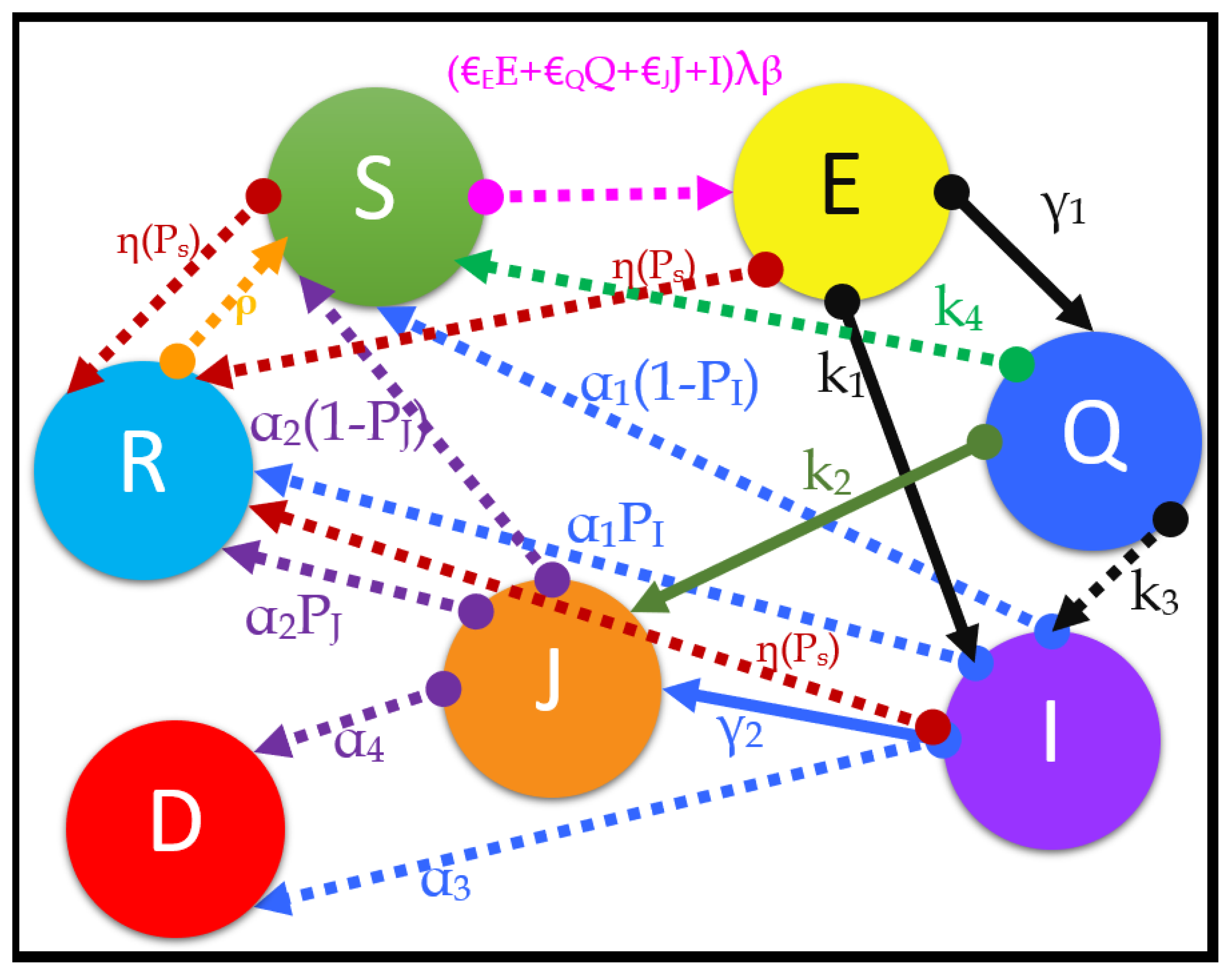
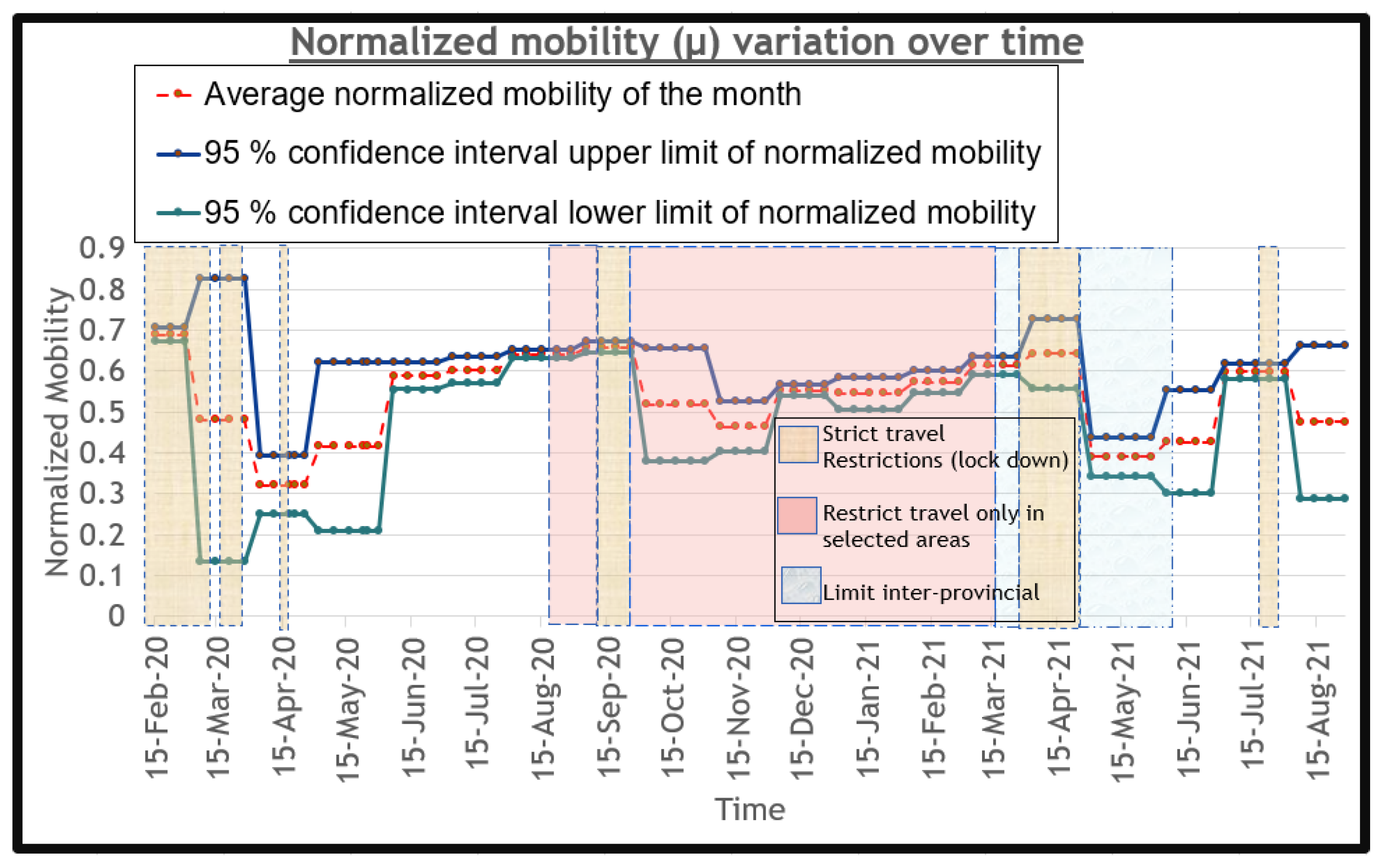
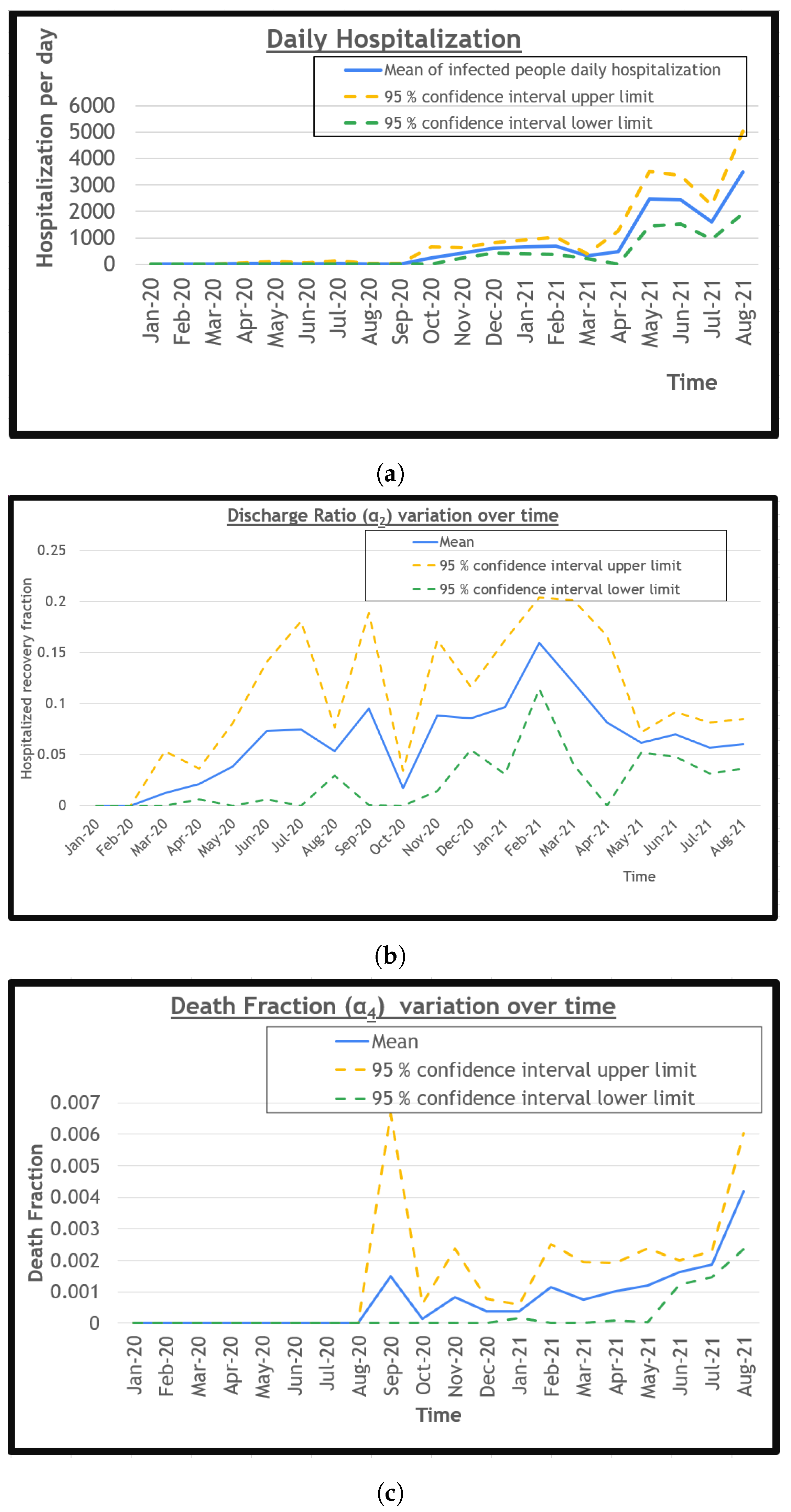
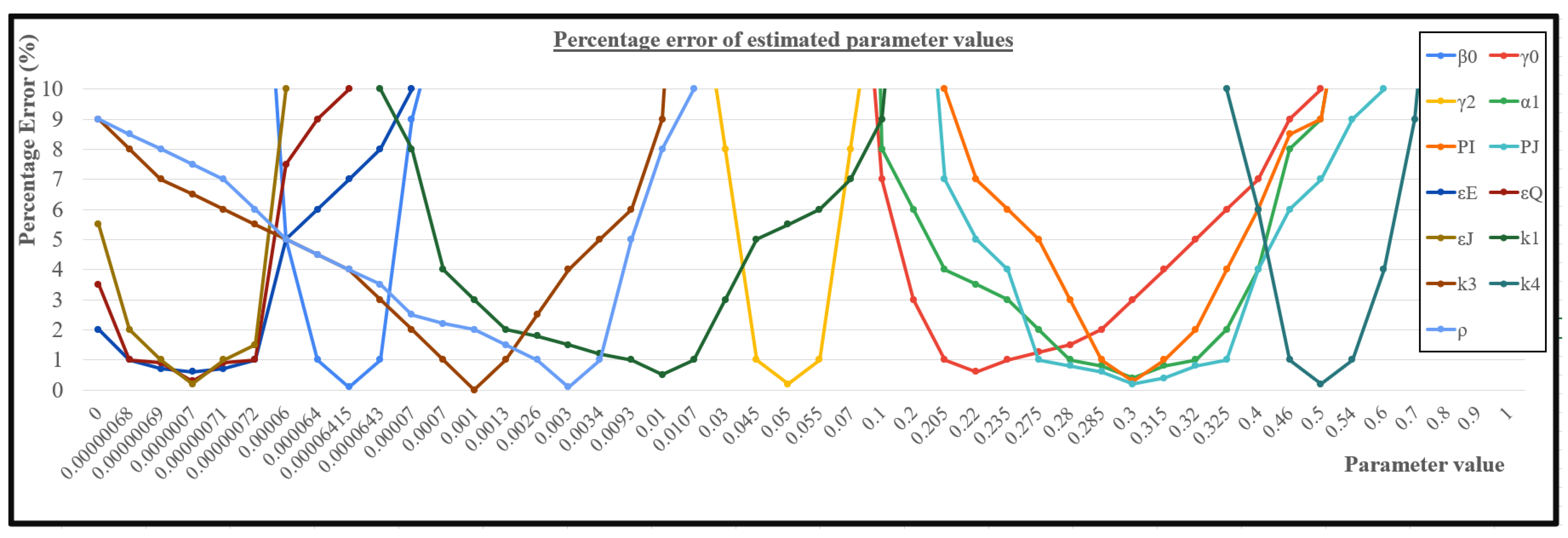
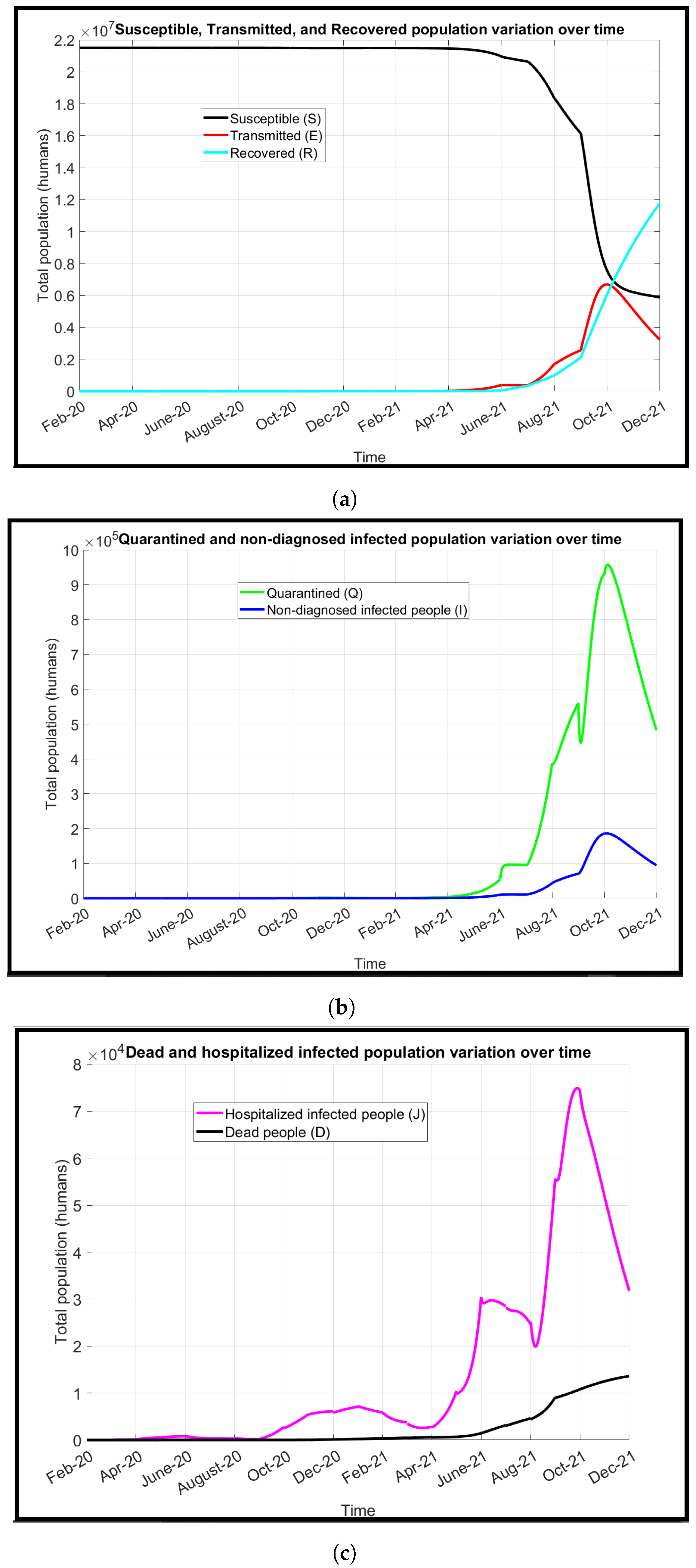
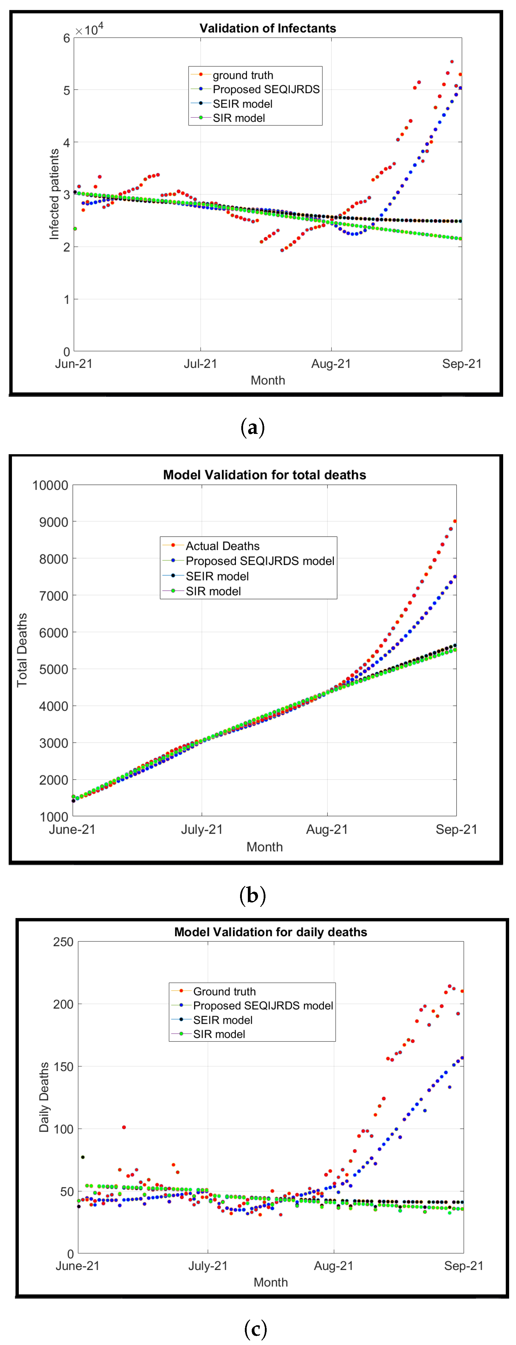
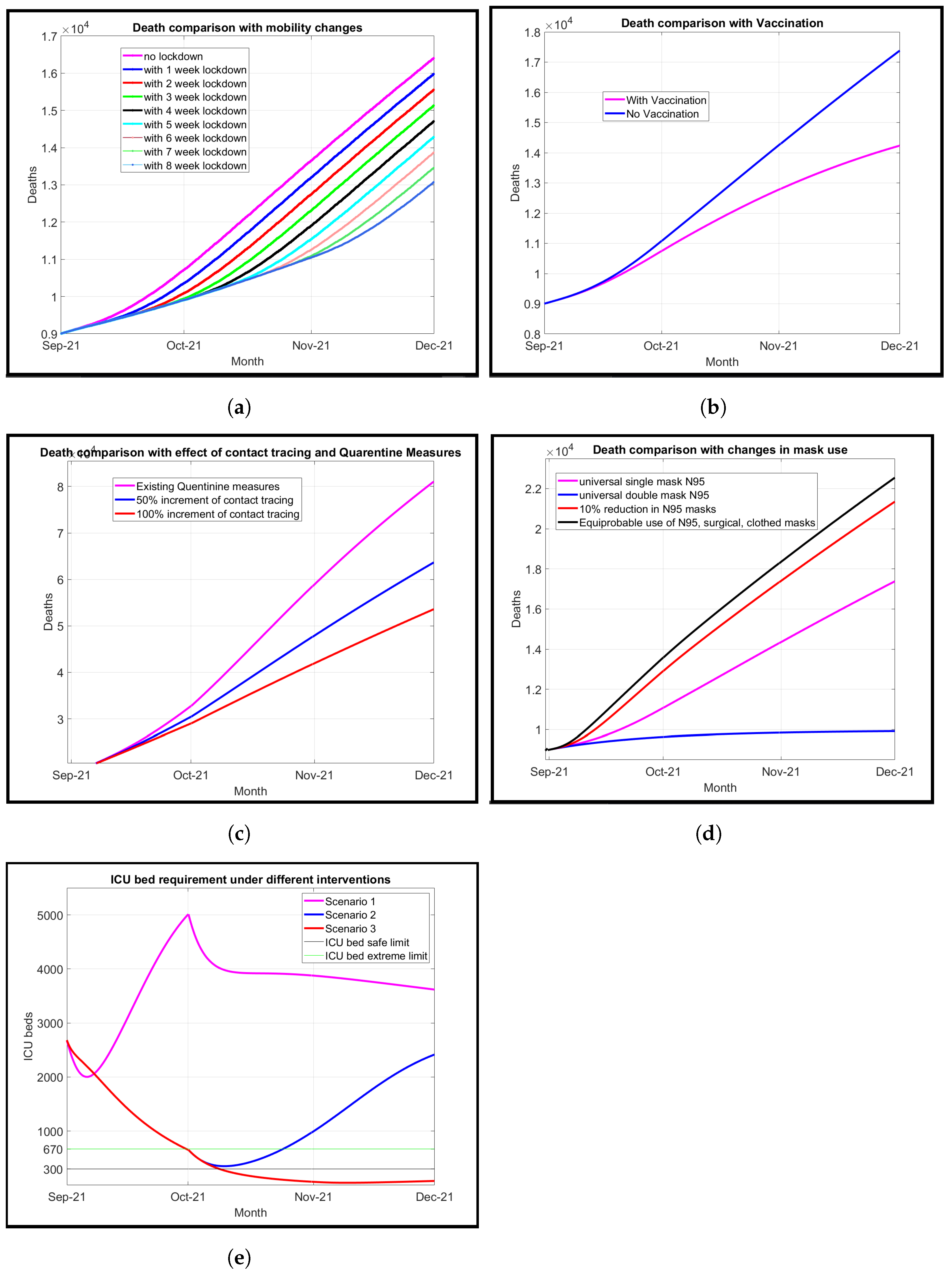
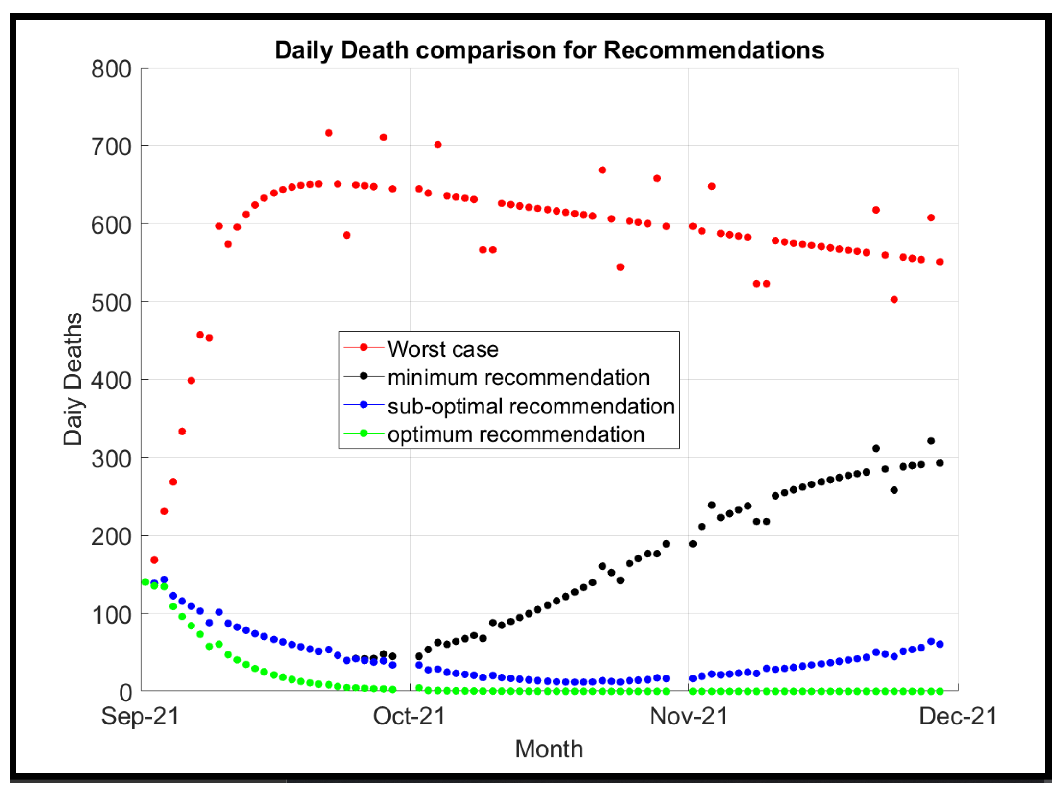
Table 1.
Table of standard mean difference effect measurements.
| SMD | Effect |
|---|---|
| SMD ≤ 0.2 | Very low |
| 0.2 < SMD ≤ 0.5 | Small |
| 0.5 < SMD ≤ 0.8 | Medium |
| SMD > 0.8 | Large |
Table 2.
Summary table of travel restrictions.
| Scenario | Start Date | End Date |
|---|---|---|
| Island-wide full lockdown | 20 March 2020 | 23 March 2020 |
| Island-wide full lockdown | 23 March 2020 | 19 April 2020 |
| Island-wide full lockdown | 23 April 2020 | 11 May 2020 |
| Island-wide full lockdown | 23 May 2020 | 26 May 2020 |
| Restrict travel in selected high-risk areas | 4 October 2020 | 18 October 2020 |
| Full lockdown in western province | 18 October 2020 | 5 November 2020 |
| Restrict travel in selected high-risk areas | 5 November 2020 | 10 May 2021 |
| Restrict inter-provincial travel | 10 May 2021 | 21 May 2021 |
| Island-wide full lockdown | 21 May 2021 | 21 June 2021 |
| Restrict inter-provincial travel | 21 June 2021 | 1 August 2021 |
Table 3.
Table of total vaccination of each dose by the end of each month.
| Dose | March | April | May | June | July | August |
|---|---|---|---|---|---|---|
| Dose 1 in M (%) | 0.91 (5.7) | 0.93 (5.8) | 1.61 (9.9) | 2.69 (16.8) | 9.63 (59.9) | 12.34 (76.7) |
| Dose 2 in M (%) | 0.0 (0.0) | 0.02 (0.1) | 0.35 (2.1) | 0.99 (6.2) | 2.13 (13.3) | 7.29 (45.3) |
Table 4.
Average first and second dose vaccination rates among different types; all vaccines with time axis shifted by 1 month.
Table 4.
Average first and second dose vaccination rates among different types; all vaccines with time axis shifted by 1 month.
| Vaccine | April | May | June | July | August | September |
|---|---|---|---|---|---|---|
| AstraZeneca | 0.00137, 0.00000 | 0.00002, 0.00004 | 0.00000, 0.00048 | 0.00000, 0.00005 | 0.00000, 0.00002 | 0.00067, 0.00075 |
| Sinopharm | 0.00000, 0.00000 | 0.00000, 0.00000 | 0.00100, 0.00000 | 0.00154, 0.00094 | 0.00897, 0.00169 | 0.00313, 0.00573 |
| Sputnik V | 0.00000, 0.00000 | 0.00000, 0.00000 | 0.00002, 0.00000 | 0.00015, 0.00002 | 0.00007, 0.00000 | 0.00000, 0.00002 |
| Pfizer | 0.00000, 0.00000 | 0.00000, 0.00000 | 0.00000, 0.00000 | 0.00000, 0.00000 | 0.00030, 0.00000 | 0.00016, 0.00028 |
| Moderna | 0.00000, 0.00000 | 0.00000, 0.00000 | 0.00000, 0.00000 | 0.00000, 0.00000 | 0.00107, 0.00000 | 0.00009, 0.00097 |
| Overall () | 0.00137 | 0.00006 | 0.00151 | 0.00269 | 0.01211 | 0.01179 |
Table 5.
Summary table of the COVID-19 variants found in Sri Lanka.
| Variant Name | Earliest Date of Detection | Relative Transmissibility () |
|---|---|---|
| B.1.411 | 2 April 2020 [60] | 1.02 [61] |
| B.1.1.7 (Alpha variant) | 2 January 2021 [62] | 1.29 [63] |
| B.1.351 (Beta variant) | 3 March 2021 [64] | 1.25 [63] |
| B.1.428 | 3 March 2021 [65] | unknown |
| B.1.617.2 (Delta variant) | 7 April 2021 [66] | 1.97 [63] |
| B.1.525 | 28 April 2021 [67] | 1.29 [63] |
| SA 222V, SA 701S, SA 1078S | 17 August 2021 [68] | unknown |
Table 6.
Table of hyperparameter values and methodology of finding the parameter values for the proposed SEQIJRDS model simulation for the COVID-19 pandemic in Sri Lanka.
Table 6.
Table of hyperparameter values and methodology of finding the parameter values for the proposed SEQIJRDS model simulation for the COVID-19 pandemic in Sri Lanka.
| Parameter | Values | Methodology |
|---|---|---|
| (0:1) | As derived in Section 2.6.7 | |
| 0.00000, 0.00137, 0.00006, 0.00151, 0.00269, 0.01211, 0.01179 | As derived in Section 2.6.8 | |
| 0.0, 0.64, 0.68, 0.66, 0.70, 0.68, 0.75 | As derived in Section 2.6.8 | |
| M | 0.01,0.05,0.145,0.31 | As derived in Section 2.6.5 and Section 3.3.4 |
| 1.0,1.02,1.25,1.29,1.97 | As derived in Section 2.6.9 | |
| 0.000006415 | Learned using model fitting for historical data | |
| 0.22 | Learned using model fitting for historical data | |
| (0:1) | As derived in Section 2.6.6 | |
| 0.05 | Learned using model fitting for historical data | |
| 0.3 | Learned using model fitting for historical data | |
| (0:1) | As derived in Section 2.6.11 | |
| (0:1) | As derived in Section 2.6.12 | |
| (0:1) | As derived in Section 2.6.12 | |
| 0.3 | Learned using model fitting for historical data | |
| 0.3 | Learned using model fitting for historical data | |
| 1.0 × 10 10 | Learned using model fitting for historical data | |
| 1.0 × 10 10 | Learned using model fitting for historical data | |
| 1.0 × 10 10 | Learned using model fitting for historical data | |
| 0.01 | Learned using model fitting for historical data | |
| (0:1) | As derived in Section 2.6.10 | |
| 0.001 | Learned using model fitting for historical data | |
| 0.5 | Learned using model fitting for historical data | |
| 0.003 | Learned using model fitting for historical data |
Table 7.
Table of mean absolute percent error comparison between the proposed SEQIJRDS, SEIR, and SIR models’ projections for hospitalized infected people.
Table 7.
Table of mean absolute percent error comparison between the proposed SEQIJRDS, SEIR, and SIR models’ projections for hospitalized infected people.
| Number of Weeks | Proposed SEQIJRDS | SIR [27] | SEIR [69] |
|---|---|---|---|
| 2 | 4.97 | 5.05 | 5.16 |
| 4 | 6.52 | 6.32 | 6.68 |
| 6 | 5.09 | 5.19 | 5.55 |
| 8 | 8.22 | 8.60 | 9.48 |
| 10 | 9.77 | 10.14 | 10.11 |
| 12 | 12.21 | 16.10 | 15.19 |
Table 8.
Table of mean absolute percent error comparison between the proposed SEQIJRDS, the SEIR, and the SIR models’ projections for cumulative deaths.
Table 8.
Table of mean absolute percent error comparison between the proposed SEQIJRDS, the SEIR, and the SIR models’ projections for cumulative deaths.
| Number of Weeks | Proposed SEQIJRDS | SIR [27] | SEIR [69] |
|---|---|---|---|
| 2 | 1.81 | 2.23 | 2.21 |
| 4 | 2.90 | 2.11 | 2.28 |
| 6 | 1.61 | 1.71 | 1.78 |
| 8 | 1.89 | 1.99 | 2.04 |
| 10 | 2.01 | 2.65 | 2.59 |
| 12 | 3.63 | 6.38 | 6.15 |
Table 9.
Table of mean absolute percent error comparison between the proposed SEQIJRDS model and the other projection models for daily deaths.
Publisher’s Note: MDPI stays neutral with regard to jurisdictional claims in published maps and institutional affiliations. |
© 2022 by the authors. Licensee MDPI, Basel, Switzerland. This article is an open access article distributed under the terms and conditions of the Creative Commons Attribution (CC BY) license (https://creativecommons.org/licenses/by/4.0/).
Share and Cite
MDPI and ACS Style
Wijesekara, P.A.D.S.N.; Wang, Y.-K. A Mathematical Epidemiological Model (SEQIJRDS) to Recommend Public Health Interventions Related to COVID-19 in Sri Lanka. COVID 2022, 2, 793-826. https://doi.org/10.3390/covid2060059
AMA Style
Wijesekara PADSN, Wang Y-K. A Mathematical Epidemiological Model (SEQIJRDS) to Recommend Public Health Interventions Related to COVID-19 in Sri Lanka. COVID. 2022; 2(6):793-826. https://doi.org/10.3390/covid2060059
Chicago/Turabian StyleWijesekara, Patikiri Arachchige Don Shehan Nilmantha, and Yu-Kai Wang. 2022. "A Mathematical Epidemiological Model (SEQIJRDS) to Recommend Public Health Interventions Related to COVID-19 in Sri Lanka" COVID 2, no. 6: 793-826. https://doi.org/10.3390/covid2060059