The Role of Orbital Nesting in the Superconductivity of Iron-Based Superconductors

Abstract

We analyze the magnetic excitations and the spin-mediated superconductivity in iron-based superconductors within a low energy model that operates in the band basis, but fully incorporates the orbital character of the spin excitations. We show how the orbital selectivity, encoded in our low energy description, simplifies substantially the analysis and allows for analytical treatments, while retaining all the main features of both spin excitations and gap functions computed using multiorbital models. Importantly, our analysis unveils the orbital matching between the hole and electron pockets as the key parameter to determine the momentum dependence and the hierarchy of the superconducting gaps, instead of the Fermi surface matching, as in the common nesting scenario.

1. Introduction

The discovery of iron-based superconductors (IBSs) raised immediate questions about the nature of the superconducting (SC) state and the pairing mechanism. From the very beginning, it was proposed that pairing could be unconventional [1,2]. This proposal was triggered by both the small estimated value of the electron–phonon coupling [3] and the proximity in the phase diagram of a magnetic instability nearby the SC one. Within a band nesting scenario, pairing is provided by repulsive spin fluctuations between hole and electron pockets, connected by the same wave vector characteristic of the spin modulations in the magnetic phase [4]. Given the repulsive and interband character of the interaction, the expected symmetry for the gap function is the so-called $s_{\pm }$, i.e., an isotropic s-wave on each pocket with opposite signs for hole and electron pockets. This picture has been supported and confirmed by extensive theoretical works that, within realistic multiorbital interacting models for IBSs, provide a quantitative estimate of the SC properties starting from a random phase approximation (RPA)-based description of the spin-susceptibility [5,6,7,8,9,10,11].

The inclusion of the orbital degree of freedom in the analysis of the SC gaps allows reproducing a number of features experimentally observed in IBSs [12] such as the angular modulation of the $s_{\pm }$ gap functions and the possibility of accidental nodes on the Fermi surfaces. On the other hand, the number of orbitals included makes the analysis of superconductivity within multiorbital models very complex. As a consequence, analytical treatments of the problems are often unattainable and the physical interpretation of the results is not straightforward. Another issue with the RPA analysis of multiorbital models is that the investigation of fluctuation-driven phenomena such as nematicity requires the inclusion of fluctuations beyond RPA [13,14], which leads to the definition of a tensorial spin nematic order parameter. In that respect, it was shown in [13,15] that reducing the number of orbitals involved in the calculations by projecting the interaction at low energy allows defining a minimal model that describes the spin nematic phase within a simple multiband language while at the same time retaining the orbital information. The low-energy projection, in fact, results in a strong orbital selectivity of the magnetic excitation with spin fluctuation along $x/y$ having a $yz/xz$ orbital character.

In this work, we performed RPA calculations of the magnetic excitations of the orbital selective spin fluctuation (OSSF) model in the tetragonal phase of IBSs. By comparing our results to analogous microscopic five-orbital calculations, we show that the OSSF model reproduces all the relevant features characterizing the RPA spin susceptibilities obtained within multiorbital models. The analysis of the SC vertex mediated by OSSF and of the corresponding gap equations results in anisotropic $s_{\pm }$ gap functions that can present accidental nodes in agreement with multiorbital calculations and experiments [11,12], as well as an SC $d_{x^2-y^2}$ state nearly degenerate with the $s_{\pm }$, as previously discussed in, e.g., [5,9]. The main advantage of the simplified description provided by the OSSF model is that a precise connection between the features of the gap functions and the orbital make-up of the nested Fermi surfaces can be made. Our analysis demonstrates that the degree of orbital nesting is the parameter that controls the modulation and the hierarchy of the SC gaps. This last observation counters the naive expectation of stronger pairing between matching Fermi surfaces and forces us to revise the band nesting paradigm in the light of the orbital degree of freedom.

2. The Orbital Selective Spin Fluctuations Model

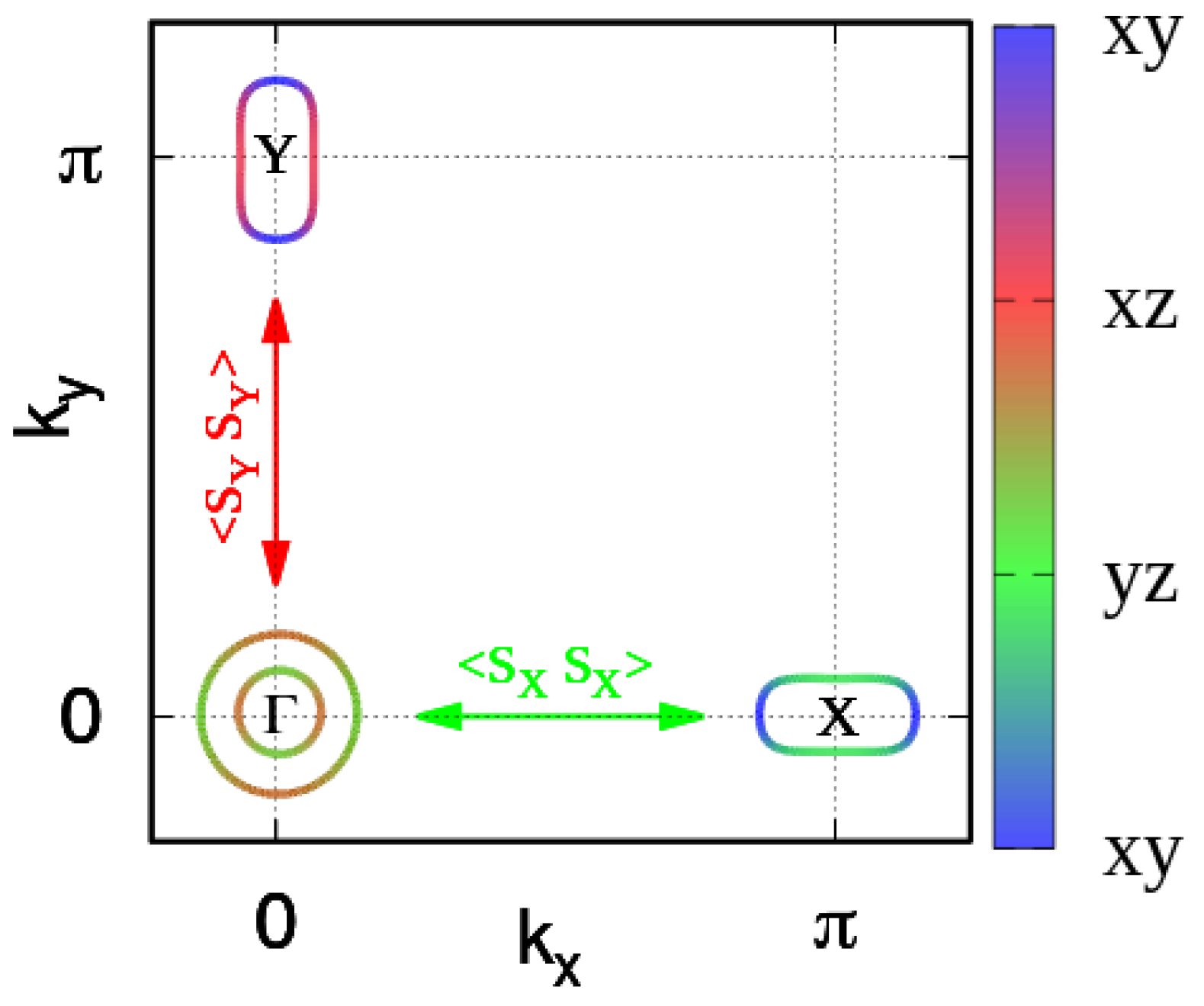
We start briefly by revising the distinctive features of the low-energy OSSF model originally derived in [15]. We considered a general four-pocket model with two hole pockets at $\mathsf{\Gamma }$, ${\mathsf{\Gamma }}_{\pm }$ and two electron pockets at X and Y; see Figure 1. Mostly three orbitals contribute to the Fermi surface, $yz$ and $xz$ for the ${\mathsf{\Gamma }}_{\pm }$ pockets and $xy$ and $yz/xz$ for the $X/Y$ pockets. The particular orbital arrangement follows from the space group of the iron plane [16]. A crucial consequence of this orbital composition is that the hole pockets ${\mathsf{\Gamma }}_{\pm }$ present opposite orbital nesting with the electron pockets, i.e., there is orbital mismatch between ${\mathsf{\Gamma }}_{+}$ and $X/Y$ and orbital match between ${\mathsf{\Gamma }}_{-}$ and $X/Y$.

The kinetic Hamiltonian is derived by adapting the low energy model considered in [16], which accounts for the orbital symmetry of the system. Each pocket is described using a spinor representation in the pseudo-orbital space:

$$H_0^l=\sum _{\mathbf{k},\sigma }{\psi }_{\mathbf{k}\sigma }^{l,†}{\widehat{H}}_0^l{\psi }_{\mathbf{k}\sigma }^l,$$

(1)

where the spinors are defined as ${\psi }^{\mathsf{\Gamma }}=(c_{yz},c_{xz})$ and ${\psi }^{X/Y}=(c_{yz/xz},c_{xy})$, ${\widehat{H}}_0^l=h_0^l{\tau }_0+{\overrightarrow{h}}^l·\overrightarrow{\tau }$, $l=\mathsf{\Gamma },X,Y$ and the $\tau$ matrices represent the pseudo-orbital spin. Diagonalizing ${\widehat{H}}_0$, we find the dispersion relations $E^{l\pm }=h_0^l\pm h^l$ with $h^l=|{\overrightarrow{h}}^l|$. We introduce the rotation from the orbital to the band basis,

$$\left(\begin{array}{c}{h}_{+}\\ h_{-}\end{array}\right)=\left(\begin{array}{cc}{u}_{\mathsf{\Gamma }}& -v_{\mathsf{\Gamma }}\\ v_{\mathsf{\Gamma }}& u_{\mathsf{\Gamma }}\end{array}\right)\left(\begin{array}{c}{c}_{yz}\\ c_{xz}\end{array}\right)$$

(2)

with an analogous expression for the $X/Y$ pockets, provided that the corresponding orbital spinor is used. At $X/Y$, only the $E^{X/Y+}$ band crosses the Fermi level, so in the following, we use $e_{X/Y}$ for the corresponding fermionic operators, dropping the + superscript. The explicit expressions of $(h_0^l,{\overrightarrow{h}}^l)$ that reproduce a four-pocket model as the one shown in Figure 1 are detailed in Appendix A. Notice that in order to lift the degeneracy of the inner and outer $xz/yz$ pockets at $\mathsf{\Gamma }$, we need to account for the spin–orbit coupling in the Hamiltonian. We added it explicitly by replacing $h^{\mathsf{\Gamma }}\to \sqrt{{\left(h^{\mathsf{\Gamma }}\right)}^2+{\lambda }^2/4}$ in the expression for $E^{{\mathsf{\Gamma }}^{\pm }}$. The kinetic model we considered here can be easily extended to account for a more general five-pocket model that includes the $xy$ hole pocket at $(\pi ,\pi )$. This band is close to the Fermi level in IBS and it crosses the Fermi level in some specific cases only, e.g., heavily hole-doped systems. We will discuss the extension of the OSSF model for a five-pocket model in a future work; however, it is worth mentioning that the conclusion discussed here based on our RPA analysis is not expected to change qualitatively once the additional pocket is taken into account.

The interacting Hamiltonian in the spin channel is:

$$H_{int}=-1/2\sum _{\mathbf{q}}{U}_{\eta {\eta }^{\prime }}{\overrightarrow{S}}^{\eta }\left(\mathbf{q}\right)·{\overrightarrow{S}}^{{\eta }^{\prime }}(-\mathbf{q}).$$

(3)

$\eta ,{\eta }^{\prime }=yz,xz,xy$ are orbital indices and $U_{\eta {\eta }^{\prime }}\sim U{\delta }_{\eta {\eta }^{\prime }}+J_H(1-{\delta }_{\eta {\eta }^{\prime }})$, with U and $J_H$ being the usual Hubbard and Hund couplings. We considered only spin operators with an intraorbital character ${\overrightarrow{S}}^{\eta }\left(\mathbf{q}\right)={\sum }_{\mathbf{k}s{s}^{\prime }}{c}_{\mathbf{k}s}^{\eta †}{\overrightarrow{\sigma }}_{s{s}^{\prime }}{c}_{\mathbf{k}+\mathbf{q}{s}^{\prime }}^{\eta }$ with ${\sigma }_{s{s}^{\prime }}$ being the Pauli matrices for the spin operator being $s,s^{\prime }$ spin indices. This choice was motivated by the general finding that the intraorbital magnetism is the dominant channel in IBSs [5,17,18,19,20]. Notice that, in order to simplify the notation, we implicitly assumed any momentum summation normalized via a $1/N$ factor where N is the number of $\mathbf{k}$-points. At low energy, we can project out the general interaction, Equation (3), onto the fermionic excitations defined by the model Equation (1). By using the rotation to the band basis, Equation (2), one can then establish a precise correspondence between the orbital and momentum character of the spin operators ${\overrightarrow{S}}_{X/Y}^{\eta }\equiv {\overrightarrow{S}}^{\eta }\left(\mathbf{q}={\mathbf{Q}}_{X/Y}\right)$:

$$\begin{array}{ccc}\hfill {\overrightarrow{S}}_X^{yz}& =& \sum _{\mathbf{k}}(u_{\mathsf{\Gamma }}{h}_{+}^{†}+v_{\mathsf{\Gamma }}{h}_{-}^{†})\overrightarrow{\sigma }{u}_X{e}_X\hfill \end{array}$$

(4)

$$\begin{array}{ccc}\hfill {\overrightarrow{S}}_Y^{xz}& =& \sum _{\mathbf{k}}(-v_{\mathsf{\Gamma }}{h}_{+}^{†}+u_{\mathsf{\Gamma }}{h}_{-}^{†})\overrightarrow{\sigma }{u}_Y{e}_Y\hfill \end{array}$$

(5)

where we only focus on the spin exchange between hole and electron pockets occurring at momenta $\mathbf{q}$ near ${\mathbf{Q}}_X$ or ${\mathbf{Q}}_Y$ and we drop for simplicity the momentum and spin indices of the fermionic operators. The interacting Hamiltonian Equation (3) reduces to:

$$H_{int}=-\frac{\tilde{U}}{2}{\overrightarrow{S}}_{X/Y}^{yz/xz}·{\overrightarrow{S}}_{X/Y}^{yz/xz}$$

(6)

where $\tilde{U}$ is the effective interaction for the low energy model. In the RPA analysis that we perform in the following, we use $\tilde{U}$ close to the critical U value at which the spin RPA susceptibility diverges, leading to the $(\pi ,0)$ magnetic order. Notice that Equation (6) is the projection of the generic interaction Hamiltonian Equation (3) onto the low energy model Equation (1). Such a projection is key to generate the OSSF. In fact, since at low energy, the $yz/xz$ fermionic states exist only around ${\mathbf{Q}}_X/{\mathbf{Q}}_Y$, it turns out that the spin operators ${\overrightarrow{S}}_X^{\eta }$ with $\eta \ne yz$ and ${\overrightarrow{S}}_Y^{\eta }$ with $\eta \ne xz$ are absent in Equation (6), and there are no terms involving Hund’s coupling.

The orbital selective character of the low-energy spin excitations makes the interacting Hamiltonian for the spin channel, Equation (6), considerably simpler than the one obtained within a five-orbital model (see, e.g., [5]). As a matter of fact, Equation (6), while retaining the orbital dependence of the spin excitations, does not acquire a complex tensorial form and is instead formally equivalent to the spin–spin interacting Hamiltonian written in the band basis $H_{int}^{band}\sim -\tilde{U}{\overrightarrow{S}}_{X/Y}·{\overrightarrow{S}}_{X/Y}$ (see, e.g., [21]). This implies that one can analyze the spin nematic phase following the same strategy of [21], in which the nematic instability was studied within an effective action derivation as a precursor effect of magnetism. The consequences of the inclusion of the orbital degree of freedom within a spin nematic action have been widely discussed especially in the analysis of the nematic phase of FeSe [15,22,23,24].

In what follows, we focus on the analysis of the superconductivity mediated by the OSSF in the tetragonal phase for a generic four-pocket model representative of IBSs. We show that the orbital selectivity of the spin fluctuations makes the RPA treatment extremely simple with respect to multiorbital calculations. Given the intraorbital scalar character of the OSSF, the analysis turns out to be mathematically equivalent to the study of single-band systems, while retaining all the multiband and multiorbital information.

3. Results

Within standard RPA analysis, the pairing is assumed to be mediated by spin and charge fluctuations [2,5,8,9]. It has been shown that for IBSs, the charge susceptibility is more than one order of magnitude smaller than the spin susceptibility (see, e.g., [5]); therefore, hereafter, we focus on the spin channel only.

The spin susceptibility for a generic multiorbital system is a four-orbital-index tensor, ${\chi }_{\delta {\delta }^{\prime }}^{\eta {\eta }^{\prime }}(\mathbf{q},\mathrm{\Omega })$. This is obtained from the analytical continuation $i{\mathrm{\Omega }}_m\to \mathrm{\Omega }+i{0}^{+}$ of the Matsubara spin–spin correlation function:

$${\chi }_{\delta {\delta }^{\prime }}^{\eta {\eta }^{\prime }}(\mathbf{q},i{\mathrm{\Omega }}_m)={\int }_0^{\beta }d\tau e^{i{\mathrm{\Omega }}_m\tau }〈T_{\tau }{\overrightarrow{S}}^{\eta \delta }(\mathbf{q},\tau ){\overrightarrow{S}}^{{\eta }^{\prime }{\delta }^{\prime }}(-\mathbf{q},0)〉$$

(7)

where $\mathbf{q}$ is the momentum vector, $\beta =1/k_{B}T$ is the inverse temperature, $\tau$ is the imaginary time, and ${\mathrm{\Omega }}_m=2m\pi k_{B}T$ is the bosonic Matsubara frequency. The spin operator in the orbital space for the $\eta ,\delta$ orbitals is defined as ${\overrightarrow{S}}^{\eta \delta }(\mathbf{q},\tau )={\sum }_{\mathbf{k}s{s}^{\prime }}{c}_{\mathbf{k}s}^{\eta †}{\overrightarrow{\sigma }}_{s{s}^{\prime }}{c}_{\mathbf{k}+\mathbf{q}{s}^{\prime }}^{\delta }$ with ${\overrightarrow{\sigma }}_{s{s}^{\prime }}$ the Pauli matrices for the spin operator. Using this explicit definition of ${\overrightarrow{S}}^{\eta \delta }$ and applying Wick’s theorem to Equation (7), the noninteracting spin susceptibility can be rewritten as:

$${\chi }_{\delta {\delta }^{\prime }}^{\eta {\eta }^{\prime }}(\mathbf{q},{\mathrm{\Omega }}_m)=-\frac{1}{\beta }\sum _{\mathbf{k},n}Tr\left[G^{\delta \eta }(\mathbf{k},i{\omega }_n)G^{{\delta }^{\prime }{\eta }^{\prime }}(\mathbf{k}+\mathbf{q},i{\omega }_n+i{\mathrm{\Omega }}_m)\right]$$

(8)

where the spectral representation of the Green function is given by the rotation to the orbital basis of the noninteracting Green function in the band basis:

$$G^{\delta \eta }(\mathbf{k},i{\omega }_n)=\sum _m\frac{a_m^{\delta }\left(\mathbf{k}\right)a_m^{\eta *}\left(\mathbf{k}\right)}{i{\omega }_n-E_m\left(\mathbf{k}\right)}$$

(9)

where ${\omega }_n=(2n+1)\pi k_{B}T$ is the fermionic Matsubara frequency and $a_m^{\eta }\left(\mathbf{k}\right)$ the matrix elements connecting the orbital ($\eta$) and the band space (m) determined by diagonalization of the tight-binding Hamiltonian. Performing the Matsubara frequency summation and setting $\mathrm{\Omega }\to 0$, the static spin susceptibility reads:

$${\chi }_{\delta {\delta }^{\prime }}^{\eta {\eta }^{\prime }}\left(\mathbf{q}\right)=-\sum _{\mathbf{k},mn}\frac{a_m^{\delta }\left(\mathbf{k}\right)a_m^{\eta *}\left(\mathbf{k}\right)a_n^{{\eta }^{\prime }*}(\mathbf{k}+\mathbf{q})a_n^{{\delta }^{\prime }}(\mathbf{k}+\mathbf{q})}{E_n(\mathbf{k}+\mathbf{q})-E_m\left(\mathbf{k}\right)}f\left(E_n(\mathbf{k}+\mathbf{q})\right)-f\left(E_m\left(\mathbf{k}\right)\right)$$

(10)

with f(E_m(k)) the Fermi distribution function. The RPA spin fluctuation is given in the form of a Dyson-type equation with the spin interaction $\widehat{U}$_S defined in terms of the multiorbital interaction parameters $U,U^{\prime },J$_H [2,5]. Analogously, the singlet pairing vertex driven by spin fluctuations can be computed on the low-energy sector in terms of the RPA spin susceptibility [5,25]. The variety of diagrams contributing to the SC vertex is large given the number of orbitals included, making it unfeasible to draw the possible Feynman diagrams up to orders larger than one. The gap equation for the multiorbital model can be computed numerically by taking into account the singlet pairing vertex as an eigenvalue problem in which the largest eigenvalue leads to the highest transition temperature and its eigenfunction determines the symmetry of the gap (see, e.g., [5,8,9,26]). An anisotropic sign changing s-wave, $s_{\pm }$, is found as the dominant symmetry for system parameters compatible with moderately doped IBSs, in agreement with experiments, e.g., [12,27,28,29]. A nearly degenerate $d_{x^2-y^2}$ state was discussed in [5,9] and could be relevant to explain Raman experiments in K-doped BaFe${}_2$As${}_2$[30,31,32,33], CaKFe${}_4$As${}_4$ [34], and (Li${}_{1-x}$Fe${}_x$)OHFeSe [35].

3.1. Magnetic Excitations in the OSSF Model: RPA Analysis

Within the OSSF model, the situation is substantially simplified as compared with the five-orbital RPA approach due to the orbital selectivity of the spin fluctuations. By assuming the spin operator to be intraorbital, the spin susceptibility of Equation (7) reduces to a two-orbital-index matrix:

$${\chi }^{\eta {\eta }^{\prime }}(\mathbf{q},i{\mathrm{\Omega }}_m)={\int }_0^{\beta }d\tau e^{i{\mathrm{\Omega }}_m\tau }〈T_{\tau }{\overrightarrow{S}}^{\eta }(\mathbf{q},\tau ){\overrightarrow{S}}^{{\eta }^{\prime }}(-\mathbf{q},0)〉$$

(11)

The low-energy projection further simplifies the spin susceptibility structure as the low-energy states are defined only around high symmetry points and have a well-defined orbital character described by Equation (1). As a consequence, also the Green functions are defined only for $l=\mathsf{\Gamma },X,Y$ as $G^l(\mathbf{k},i{\omega }_n)={\widehat{\mathcal{U}}}^l(\mathbf{k},i{\omega }_n)diag(g^{l_{+}}(\mathbf{k},i{\omega }_n),g^{l_{-}}(\mathbf{k},i{\omega }_n)){\widehat{\mathcal{U}}}^{l^{-1}}(\mathbf{k},i{\omega }_n)$. Here, ${\widehat{\mathcal{U}}}^l$ are the matrices that diagonalize the l-Hamiltonian and $g^{l\pm }(\mathbf{k},i{\omega }_n)={(i{\omega }_n-E_{\mathbf{k}}^{l\pm })}^{-1}$ the Green functions in the band basis. Substituting the intraorbital spin operator ${\overrightarrow{S}}^{\eta }(\mathbf{q},\tau )$ and applying Wick’s theorem to Equation (11), the intraorbital spin susceptibility in the low-energy projection can be read as:

$${\chi }^{l{l}^{\prime }}(\mathbf{q},i{\mathrm{\Omega }}_m)=-\frac{1}{\beta }\sum _{\mathbf{k},n}Tr\left[{\widehat{G}}^l(\mathbf{k},i{\omega }_n){\widehat{G}}^{l^{\prime }}(\mathbf{k}+\mathbf{q},i{\omega }_n+i{\mathrm{\Omega }}_m)\right].$$

(12)

Equation (12) represents the spin susceptibility between two pockets l and $l^{{}^{\prime }}$ and depends on the transferred momentum $\mathbf{q}={\mathbf{k}}^{\prime }-\mathbf{k}$ and the external frequency $\mathrm{\Omega }$. Performing the Matsubara frequency summation and setting $\mathrm{\Omega }\to 0$ in Equation (12), we find the static susceptibility for the $l_{\pm }$$l_{\pm }^{{}^{\prime }}$ pockets in terms of the Fermi distribution function $f\left(E_{\mathbf{k}}^{l_{\pm }}\right)$ and ${|(u/v)}^l\left(\mathbf{k}\right)|$ that are the elements of the rotational matrix ${\widehat{\mathcal{U}}}^l$ connecting the orbital and the band space:

$${\chi }_{\eta }^{l_{\pm }{l}_{\pm }^{\prime }}\left(\mathbf{q}\right)=\sum _{\mathbf{k}}\frac{f\left(E_{\mathbf{k}+\mathbf{q}}^{l_{\pm }^{\prime }}\right)-f\left(E_{\mathbf{k}}^{l_{\pm }}\right)}{E_{\mathbf{k}+\mathbf{q}}^{l_{\pm }^{\prime }}-E_{\mathbf{k}}^{l_{\pm }}}{|(u/v)}_{\mathbf{k}}^l{|}^2{|{(u/v)}_{\mathbf{k}+\mathbf{q}}^{l^{\prime }}|}^2.$$

(13)

we refer the reader to Appendix B for further details. The resulting static susceptibility Equation (13), although formally similar to the multiorbital spin susceptibility in Equation (10), is much simpler due to the orbital selectivity of the spin fluctuations. In fact, within the OSSF, the two most relevant spin susceptibilities for a four-pocket model only involve the $yz$ orbital coming from the interaction between the ${\mathsf{\Gamma }}_{\pm }$ holes with the X electron pockets and the $xz$ orbital coming from the ${\mathsf{\Gamma }}_{\pm }$ holes with the Y electron pockets near ${\mathbf{Q}}_X$ and ${\mathbf{Q}}_Y$, respectively. To better compare with the results obtained within five-orbital model calculations, in what follows, we account also for the spin susceptibility centered around ${\mathbf{Q}}_M=(\pi ,\pi )$ that describes the spin exchange between the X and Y electron pockets and, at low energy, involves the $xy$ orbital only.

The RPA spin susceptibilities are obtained in the form of Dyson-type equations. The results of the resummation read:

$${\chi }_{\eta \mathrm{RPA}}^{l_{\pm }{l}_{\pm }^{\prime }}\left(\mathbf{q}\right)=\frac{{\chi }_{\eta }^{l_{\pm }{l}_{\pm }^{\prime }}\left(\mathbf{q}\right)}{1-\tilde{U}{\chi }_{\eta }^{l_{\pm }{l}_{\pm }^{\prime }}\left(\mathbf{q}\right)}$$

(14)

with ${\chi }_{\eta }^{l_{\pm }{l}_{\pm }^{\prime }}\left(\mathbf{q}\right)$ the noninteracting spin susceptibility given by Equation (13). The set of orbital-selective RPA susceptibilities for the different pockets is given in Appendix B. Notice that, within our model Equation (6), both the low-energy effective coupling $\tilde{U}$ and the OSSF ${\chi }_{\eta }^{l_{\pm }{l}_{\pm }^{\prime }}$ are intraorbital and have a scalar character. As a consequence, the RPA spin susceptibility given by Equation (14) is straightforward and inherits the orbital selectivity and scalar form of the OSSF. As we discuss in the following Section 3.2 and Section 3.3, this aspect allowed us to derive analytical expressions for the pairing vertex and SC gaps.

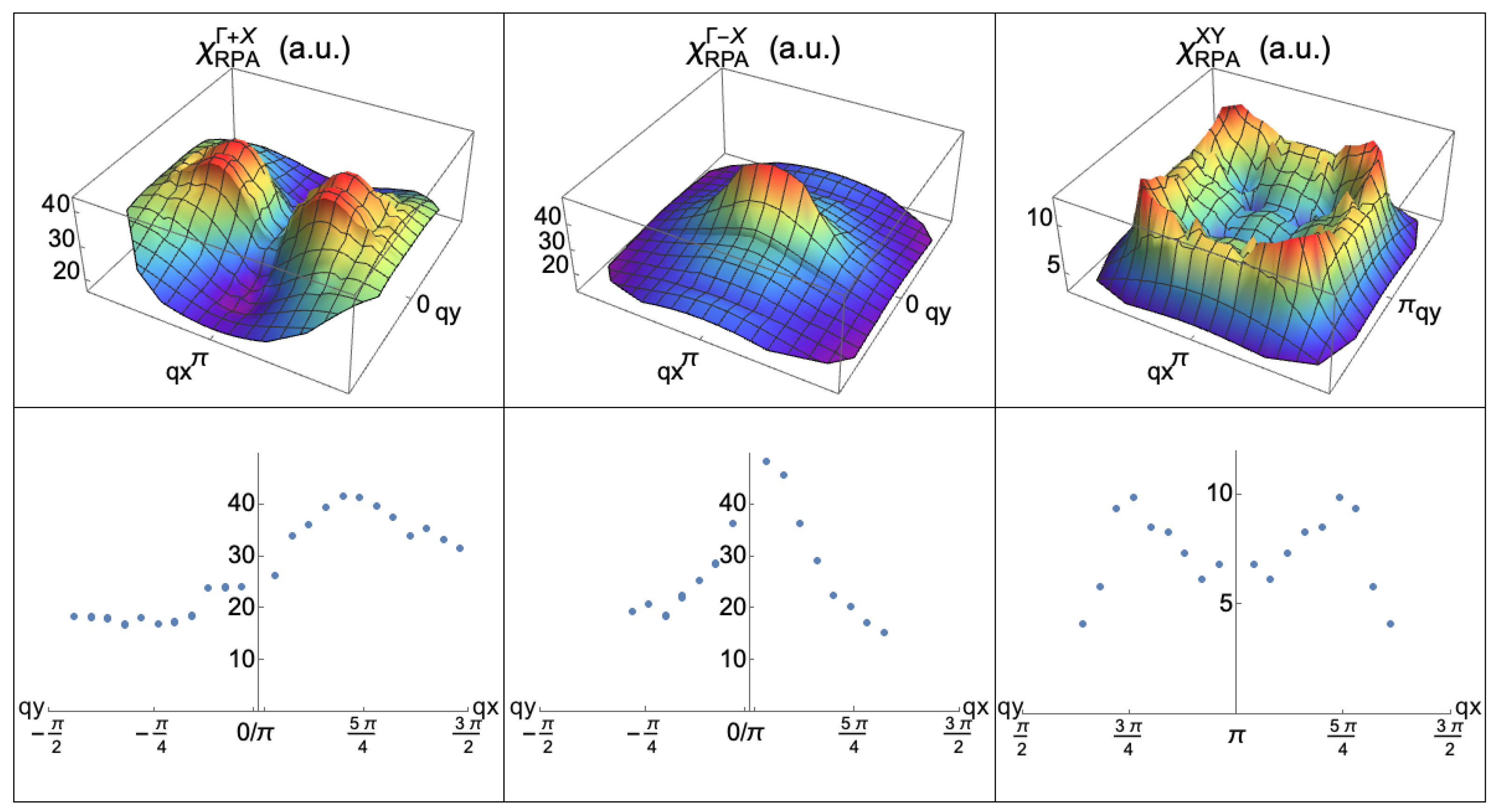
To gain insight into the previous result, we performed a numerical estimate for the RPA spin susceptibility given by Equation (14) for the four-pocket model, shown in Figure 1. We show ${\chi }_{yz\mathrm{RPA}}^{{\mathsf{\Gamma }}_{+}X}\left(\mathbf{q}\right)$, ${\chi }_{yz\mathrm{RPA}}^{{\mathsf{\Gamma }}_{-}X}\left(\mathbf{q}\right)$, and ${\chi }_{xy\mathrm{RPA}}^{XY}\left(\mathbf{q}\right)$ in Figure 2. In the upper panel, we show 3D color maps in $(q_x,q_y)$. The bottom panels show the 2D cuts along $q_x/q_y$ centered in ${\mathbf{Q}}_X=(\pi ,0)$ for the electron–hole spin susceptibilities and ${\mathbf{Q}}_M=(\pi ,\pi )$ for the electron–electron one. This representation allows easily comparing the relative weight of the different susceptibilities. Notice that the contributions of the Y pocket (not shown) are equivalent to those for the X pockets with a $\pi /2$ rotation, since in the tetragonal phase, the susceptibility is isotropic in both directions.

From Figure 2, we can highlight two main results:

(i) The orbital-selective RPA spin susceptibilities around ${\mathbf{Q}}_X$ and ${\mathbf{Q}}_M$ show a clear momentum-dependent structure of the peaks. This can be explained due to the degree of orbital nesting between pockets. The orbital nesting indicates the relative orbital composition between the two pockets involved in the spin exchange mechanism. In Figure 2, we can see that when there is an orbital mismatch, as is the case of the ${\mathsf{\Gamma }}_{+}$ and X pockets, the spin susceptibility develops two incommensurate peaks around ${\mathbf{Q}}_X$. In contrast, if there is an orbital match between pockets, i.e., the case of ${\mathsf{\Gamma }}_{-}$ and X, the spin susceptibility develops a single commensurate peak at the ${\mathbf{Q}}_X=(\pi ,0)$. For the ${\chi }_{xy\mathrm{RPA}}^{XY}\left(\mathbf{q}\right)$ susceptibility, there is a total mismatch between the $xy$ orbital of the electrons pockets. Thus, the spin susceptibility is totally incommensurate and develops four symmetric peaks that correspond to the overlaps of the $xy$ orbital contribution around the $(\pi ,\pi )$ point;

(ii) The main contribution to the spin susceptibility comes from the ${\mathbf{Q}}_{X/Y}$ spin mode, between the ${\mathsf{\Gamma }}_{-}$ and the $X/Y$ pockets. This is a consequence of the orbital composition of the nested bands. The Fermi surfaces of ${\mathsf{\Gamma }}_{-}$ and $X/Y$ are, in fact, characterized by fully matching orbitals.

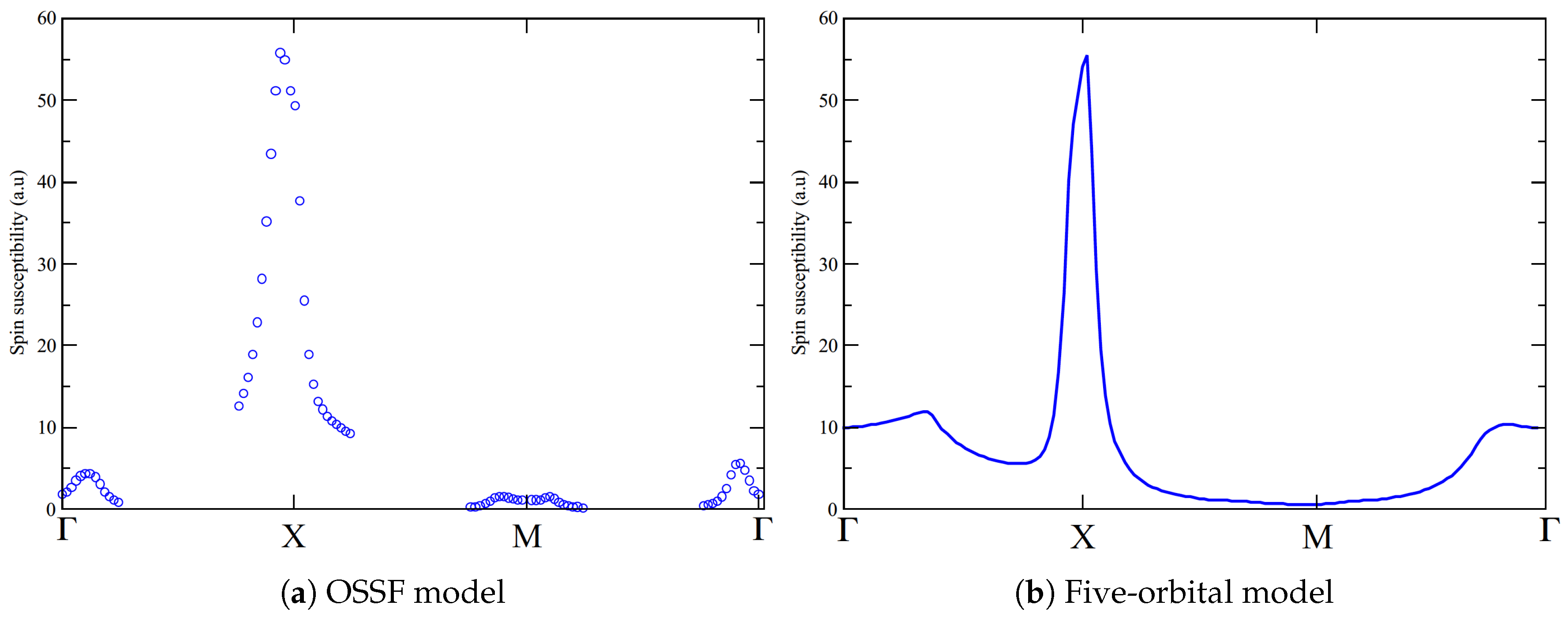
We compared our results with numerical calculations of the RPA spin susceptibility for a five-orbital model adapted from [5]. By tuning the filling and the crystal field, we can consider separately two different cases: the first one corresponds to a four-pocket model with better band nesting between the ${\mathsf{\Gamma }}_{-}$ and the electron pockets and the second case to a four-pocket model with better band nesting between the ${\mathsf{\Gamma }}_{+}$ and the $X/Y$ pockets. We obtained for the first case a commensurability of the RPA spin susceptibility at the ${\mathbf{Q}}_X=(\pi ,0)$, whereas in the second case, we obtained noncommensurate peaks around ${\mathbf{Q}}_X=(\pi ,0)$. Therefore, the same orbital modulation for the momentum dependence of the RPA spin susceptibility was obtained within the OSSF and the multiorbital models. We also computed the RPA spin susceptibility coming from the electron–electron sector within the five-orbital model. As expected, we found that the contribution from this sector was negligible in comparison with the one for the hole–electron sector [11]. It is worth noticing that, while the existence of a correlation between the orbital make-up of the Fermi surface and the momentum-dependent structure of the RPA spin excitation has already been highlighted within multiorbital models (e.g., [10]), the explicit link between orbital nesting and the momentum dependence of the spin susceptibility is made transparent within the RPA analysis of the OSSF model.

In Figure 3, we compare the cuts along the main symmetry directions of the RPA spin susceptibility (including the intraband ones) computed within the OSSF model and the multiorbital model. The calculation performed within the OSSF model reproduced remarkably well the overall momentum dependence of the spin spectrum, as well as the relative height and width of the various peaks.

This comparative analysis proved that we can obtain a reliable description of the spin spectrum within the OSSF model of Equation (13), without dealing with the tensorial form of the spin susceptibility given in the five-orbital model, Equation (10).

3.2. Superconductivity Mediated by OSSF

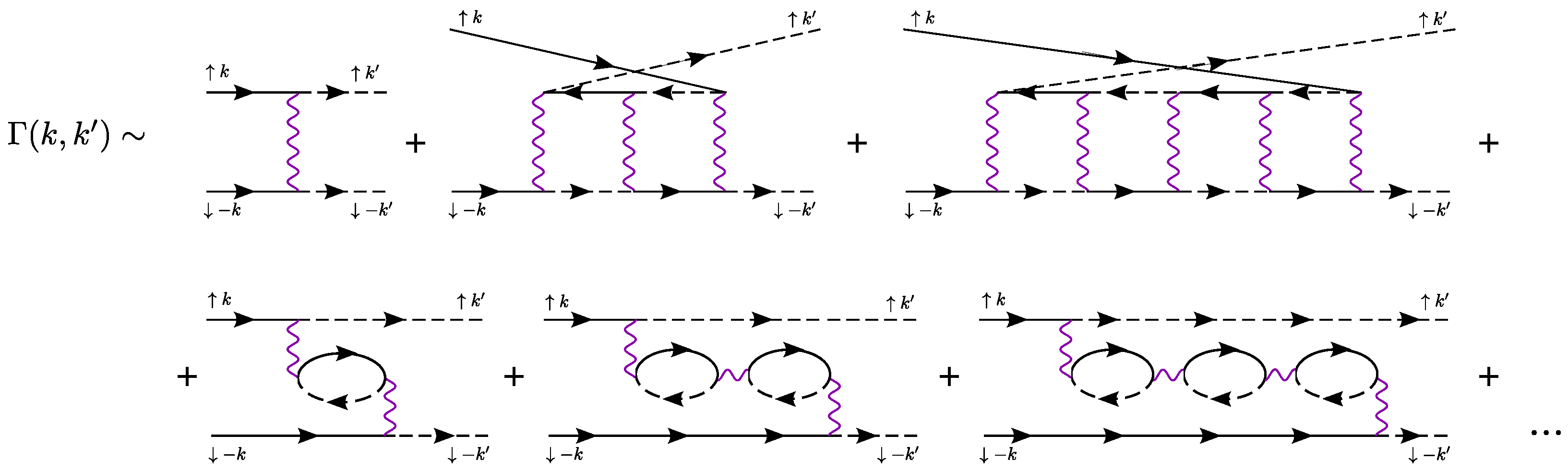
In Figure 4, we show the RPA leading diagrams for the SC vertex of electrons of opposite spin and momentum. Within the OSSF model, we can explicitly draw the Feynman diagrams up to the a finite order in $\tilde{U}$. This is possible given the intraorbital scalar character of the low-energy orbital-selective spin susceptibility that allowed us to easily perform the diagrammatic expansion explicitly. Notice that the expansion is instead practically unfeasible within the five-orbital model due to the complex tensorial structure of the pairing vertex.

As a consequence of the projection to a constrained orbital space within the OSSF model, the diagrammatic expansion for the RPA pairing vertex is formally equivalent to the one for the band basis model, which, however, does not contain the orbital information of the spin fluctuations’ exchange. Within the multiband model, the RPA pairing vertex is composed by the exchange of spin fluctuations connecting an electron pocket with a hole pocket. On the other hand, within the OSSF model, the essential difference is that the low-energy exchanged spin fluctuations connect a hole with an electron pocket with the same orbital content $yz$ or $xz$. In this way, we retain the simplicity of the analysis of the Feynman diagrams within the multiband model and, at the same time, account for the orbital degree of freedom of the system.

The leading RPA diagrams for the vertex (Figure 4) can be written as:

$${\mathsf{\Gamma }}_{\eta }^{l_{\pm }{l}_{\pm }^{\prime }}\left(\mathbf{q}\right)=\tilde{U}+\frac{{\tilde{U}}^2{\chi }_{\eta }^{l_{\pm }{l}_{\pm }^{\prime }}\left(\mathbf{q}\right)}{1-\tilde{U}{\chi }_{\eta }^{l_{\pm }{l}_{\pm }^{\prime }}\left(\mathbf{q}\right)}+\frac{{\tilde{U}}^3{\chi }_{\eta }^{{l_{\pm }{l}_{\pm }^{\prime }}^2}\left(\mathbf{q}\right)}{1-{\tilde{U}}^2{\chi }_{\eta }^{{l_{\pm }{l}_{\pm }^{\prime }}^2}\left(\mathbf{q}\right)}$$

(15)

where $\mathbf{q}={\mathbf{k}}^{\prime }-\mathbf{k}$ is the transferred momentum, $\tilde{U}$ is the intraorbital effective coupling, and ${\chi }_{\eta }^{l_{\pm }{l}_{\pm }^{\prime }}\left(\mathbf{q}\right)$ is the intraorbital susceptibility given in Equation (13). As we consider the spin channel only, the SC vertex is proportional to the RPA spin susceptibility and preserves the orbital and momentum dependencies and the physical properties discussed in the previous section. For instance, we obtained the same criterion of commensurability or incommensurability depending on the orbital matching between pockets. In the same way, we also obtained that the dominant contribution to the RPA pairing vertex was given by the spin fluctuations exchange between hole and electron pockets, the largest between pockets having matching orbitals, i.e., ${\mathsf{\Gamma }}_{-}-X/Y$.

3.3. Superconducting Gaps

We solved the BCS gap equations mediated by the OSSF for a four-pocket model for IBSs in the tetragonal phase. In order to better highlight the effect of the orbital nesting between the hole and electron nested pockets, we considered a case in which the two hole pockets are almost equivalent in size (model parameters can be found in Appendix D); see Figure 5. In this way, the degree of band nesting between the hole and electron pockets is the same for the inner and outer hole pockets, but the orbital matching condition determined by the space group of the iron plane [16] is different for ${\mathsf{\Gamma }}_{\pm }$. For simplicity, we show here the equations for the $yz$ and $xz$ components only. However, we numerically solved the full orbital system in which we also considered the SC vertex mediated by the exchange of spin fluctuations between the X and Y pockets; see Appendix C. The pairing Hamiltonian for the $yz$ and $xz$ orbital contributions reads:

$$\begin{array}{ccc}\hfill H_{yz,xz}^{pairing}& =& -\sum _{\mathbf{k},{\mathbf{k}}^{\prime }}{\mathsf{\Gamma }}_{yz\mathbf{k}{\mathbf{k}}^{\prime }}^{{\mathsf{\Gamma }}_{+}X}\left[{\left(u_{\mathbf{k}}^{\mathsf{\Gamma }}\right)}^2{h}_{\mathbf{k}}^{+†}{h}_{-\mathbf{k}}^{+†}{\left(u_{\mathbf{k}}^X\right)}^2{e}_{{\mathbf{k}}^{\prime }}^X{e}_{-{\mathbf{k}}^{\prime }}^X\right]-\sum _{\mathbf{k},{\mathbf{k}}^{\prime }}{\mathsf{\Gamma }}_{yz\mathbf{k}{\mathbf{k}}^{\prime }}^{{\mathsf{\Gamma }}_{-}X}\left[{\left(v_{\mathbf{k}}^{\mathsf{\Gamma }}\right)}^2{h}_{\mathbf{k}}^{-†}{h}_{-\mathbf{k}}^{-†}{\left(u_{\mathbf{k}}^X\right)}^2{e}_{{\mathbf{k}}^{\prime }}^X{e}_{-{\mathbf{k}}^{\prime }}^X\right]\hfill \\ & -& \sum _{\mathbf{k},{\mathbf{k}}^{\prime }}{\mathsf{\Gamma }}_{xz\mathbf{k}{\mathbf{k}}^{\prime }}^{{\mathsf{\Gamma }}_{+}Y}\left[{\left(v_{\mathbf{k}}^{\mathsf{\Gamma }}\right)}^2{h}_{\mathbf{k}}^{+†}{h}_{-\mathbf{k}}^{+†}{\left(u_{\mathbf{k}}^Y\right)}^2{e}_{{\mathbf{k}}^{\prime }}^Y{e}_{-{\mathbf{k}}^{\prime }}^Y\right]-\sum _{\mathbf{k},{\mathbf{k}}^{\prime }}{\mathsf{\Gamma }}_{xz\mathbf{k}{\mathbf{k}}^{\prime }}^{{\mathsf{\Gamma }}_{-}Y}\left[{\left(u_{\mathbf{k}}^{\mathsf{\Gamma }}\right)}^2{h}_{\mathbf{k}}^{-†}{h}_{-\mathbf{k}}^{-†}{\left(u_{\mathbf{k}}^Y\right)}^2{e}_{{\mathbf{k}}^{\prime }}^Y{e}_{-{\mathbf{k}}^{\prime }}^Y\right]+h.c.\hfill \end{array}$$

(16)

where ${\mathsf{\Gamma }}_{\eta \mathbf{k}{\mathbf{k}}^{\prime }}^{l_{\pm }{l}_{\pm }^{\prime }}$ with $\eta =yz/xz$ the RPA pairing vertex given by Equation (15) for the different pockets $l_{\pm }{l}_{\pm }^{\prime }$ and ${\left(u_{\mathbf{k}}^l\right)}^2$ and ${\left(v_{\mathbf{k}}^l\right)}^2$ are the coherence factors that connect the orbital and the band basis and account for the pockets’ orbital character.

The pairing Hamiltonian given by Equation (16) was solved in the mean field approximation by defining the orbital dependent SC order parameters for the hole sector (${\Delta }_{yz}^{{\mathsf{\Gamma }}_{+}X},{\Delta }_{yz}^{{\mathsf{\Gamma }}_{-}X},{\Delta }_{xz}^{{\mathsf{\Gamma }}_{+}Y},{\Delta }_{xz}^{{\mathsf{\Gamma }}_{-}Y}$) and for the electron sector (${\Delta }_{yz}^{X{\mathsf{\Gamma }}_{+}},{\Delta }_{yz}^{X{\mathsf{\Gamma }}_{-}},{\Delta }_{xz}^{Y{\mathsf{\Gamma }}_{+}},{\Delta }_{xz}^{Y{\mathsf{\Gamma }}_{-}}$). The resulting linearized gap equations at $T=0$ read as:

$$\begin{array}{ccc}\hfill {\Delta }_{yz{\mathbf{k}}^{\prime }}^{{\mathsf{\Gamma }}_{+}X}& =& -\sum _k\frac{{\mathsf{\Gamma }}_{yz\mathbf{k}{\mathbf{k}}^{\prime }}^{{\mathsf{\Gamma }}_{+}X}}{|v_{F\mathbf{k}}^X|}{\left(u_{\mathbf{k}}^X\right)}^4\left[{\Delta }_{yz\mathbf{k}}^{X{\mathsf{\Gamma }}_{+}}+{\Delta }_{yz\mathbf{k}}^{X{\mathsf{\Gamma }}_{-}}\right]\hfill \end{array}$$

(17)

$$\begin{array}{ccc}\hfill {\Delta }_{yz{\mathbf{k}}^{\prime }}^{{\mathsf{\Gamma }}_{-}X}& =& -\sum _k\frac{{\mathsf{\Gamma }}_{yz\mathbf{k}{\mathbf{k}}^{\prime }}^{{\mathsf{\Gamma }}_{-}X}}{|v_{F\mathbf{k}}^X|}{\left(u_{\mathbf{k}}^X\right)}^4\left[{\Delta }_{yz\mathbf{k}}^{X{\mathsf{\Gamma }}_{+}}+{\Delta }_{yz\mathbf{k}}^{X{\mathsf{\Gamma }}_{-}}\right]\hfill \end{array}$$

(18)

$$\begin{array}{ccc}\hfill {\Delta }_{xz{\mathbf{k}}^{\prime }}^{{\mathsf{\Gamma }}_{+}Y}& =& -\sum _k\frac{{\mathsf{\Gamma }}_{xz\mathbf{k}{\mathbf{k}}^{\prime }}^{{\mathsf{\Gamma }}_{+}Y}}{|v_{F\mathbf{k}}^Y|}{\left(u_{\mathbf{k}}^Y\right)}^4\left[{\Delta }_{xz\mathbf{k}}^{Y{\mathsf{\Gamma }}_{+}}+{\Delta }_{xz\mathbf{k}}^{Y{\mathsf{\Gamma }}_{-}}\right]\hfill \end{array}$$

(19)

$$\begin{array}{ccc}\hfill {\Delta }_{xz{\mathbf{k}}^{\prime }}^{{\mathsf{\Gamma }}_{-}Y}& =& -\sum _k\frac{{\mathsf{\Gamma }}_{xz\mathbf{k}{\mathbf{k}}^{\prime }}^{{\mathsf{\Gamma }}_{-}Y}}{|v_{F\mathbf{k}}^Y|}{\left(u_{\mathbf{k}}^Y\right)}^4\left[{\Delta }_{xz\mathbf{k}}^{Y{\mathsf{\Gamma }}_{+}}+{\Delta }_{xz\mathbf{k}}^{Y{\mathsf{\Gamma }}_{-}}\right]\hfill \end{array}$$

(20)

$$\begin{array}{ccc}\hfill {\Delta }_{yz{\mathbf{k}}^{\prime }}^{X{\mathsf{\Gamma }}_{+}}& =& -\sum _k\frac{{\mathsf{\Gamma }}_{yz\mathbf{k}{\mathbf{k}}^{\prime }}^{{\mathsf{\Gamma }}_{+}X}}{|v_{F\mathbf{k}}^{h_{+}}|}{\left(u_{\mathbf{k}}^{\mathsf{\Gamma }}\right)}^2\left[{\left(u_{\mathbf{k}}^{\mathsf{\Gamma }}\right)}^2{\Delta }_{yz\mathbf{k}}^{{\mathsf{\Gamma }}_{+}X}+{\left(v_{\mathbf{k}}^{\mathsf{\Gamma }}\right)}^2{\Delta }_{xz\mathbf{k}}^{{\mathsf{\Gamma }}_{+}Y}\right]\hfill \end{array}$$

(21)

$$\begin{array}{ccc}\hfill {\Delta }_{yz{\mathbf{k}}^{\prime }}^{X{\mathsf{\Gamma }}_{-}}& =& -\sum _k\frac{{\mathsf{\Gamma }}_{yz\mathbf{k}{\mathbf{k}}^{\prime }}^{{\mathsf{\Gamma }}_{-}X}}{|v_{F\mathbf{k}}^{h_{-}}|}{\left(v_{\mathbf{k}}^{\mathsf{\Gamma }}\right)}^2\left[{\left(v_{\mathbf{k}}^{\mathsf{\Gamma }}\right)}^2{\Delta }_{yz\mathbf{k}}^{{\mathsf{\Gamma }}_{-}X}+{\left(u_{\mathbf{k}}^{\mathsf{\Gamma }}\right)}^2{\Delta }_{xz\mathbf{k}}^{{\mathsf{\Gamma }}_{-}Y}\right]\hfill \end{array}$$

(22)

$$\begin{array}{ccc}\hfill {\Delta }_{xz{\mathbf{k}}^{\prime }}^{Y{\mathsf{\Gamma }}_{+}}& =& -\sum _k\frac{{\mathsf{\Gamma }}_{xz\mathbf{k}{\mathbf{k}}^{\prime }}^{{\mathsf{\Gamma }}_{+}Y}}{|v_{F\mathbf{k}}^{h_{+}}|}{\left(v_{\mathbf{k}}^{\mathsf{\Gamma }}\right)}^2\left[{\left(u_{\mathbf{k}}^{\mathsf{\Gamma }}\right)}^2{\Delta }_{yz\mathbf{k}}^{{\mathsf{\Gamma }}_{+}X}+{\left(v_{\mathbf{k}}^{\mathsf{\Gamma }}\right)}^2{\Delta }_{xz\mathbf{k}}^{{\mathsf{\Gamma }}_{+}Y}\right]\hfill \end{array}$$

(23)

$$\begin{array}{ccc}\hfill {\Delta }_{xz{\mathbf{k}}^{\prime }}^{Y{\mathsf{\Gamma }}_{-}}& =& -\sum _k\frac{{\mathsf{\Gamma }}_{xz\mathbf{k}{\mathbf{k}}^{\prime }}^{{\mathsf{\Gamma }}_{-}Y}}{|v_{F\mathbf{k}}^{h_{-}}|}{\left(u_{\mathbf{k}}^{\mathsf{\Gamma }}\right)}^2\left[{\left(v_{\mathbf{k}}^{\mathsf{\Gamma }}\right)}^2{\Delta }_{yz\mathbf{k}}^{{\mathsf{\Gamma }}_{-}X}+{\left(u_{\mathbf{k}}^{\mathsf{\Gamma }}\right)}^2{\Delta }_{xz\mathbf{k}}^{{\mathsf{\Gamma }}_{-}Y}\right]\hfill \end{array}$$

(24)

with $v_{F\mathbf{k}}^l={\partial }_{\mathbf{k}}\left({ϵ}_{\mathbf{k}}^{l\pm }\right)$ the Fermi velocity for the pocket l. Equations (17)–(24) represent the orbital components for each gap. Then, we define the total low-energy band gaps ${\Delta }_{\mathbf{k}}^l$ as:

$$\begin{array}{ccc}\hfill {\Delta }_{\mathbf{k}}^{{\mathsf{\Gamma }}_{+}}& =& {\left(u_{\mathbf{k}}^{\mathsf{\Gamma }}\right)}^2{\Delta }_{yz\mathbf{k}}^{{\mathsf{\Gamma }}_{+}X}+{\left(v_{\mathbf{k}}^{\mathsf{\Gamma }}\right)}^2{\Delta }_{xz\mathbf{k}}^{{\mathsf{\Gamma }}_{+}Y}\hfill \end{array}$$

(25)

$$\begin{array}{ccc}\hfill {\Delta }_{\mathbf{k}}^{{\mathsf{\Gamma }}_{-}}& =& {\left(v_{\mathbf{k}}^{\mathsf{\Gamma }}\right)}^2{\Delta }_{yz\mathbf{k}}^{{\mathsf{\Gamma }}_{-}X}+{\left(u_{\mathbf{k}}^{\mathsf{\Gamma }}\right)}^2{\Delta }_{xz\mathbf{k}}^{{\mathsf{\Gamma }}_{-}Y}\hfill \end{array}$$

(26)

$$\begin{array}{ccc}\hfill {\Delta }_{\mathbf{k}}^X& =& {\left(u_{\mathbf{k}}^X\right)}^2({\Delta }_{yz\mathbf{k}}^{X{\mathsf{\Gamma }}_{+}}+{\Delta }_{yz\mathbf{k}}^{X{\mathsf{\Gamma }}_{-}})\hfill \end{array}$$

(27)

$$\begin{array}{ccc}\hfill {\Delta }_{\mathbf{k}}^Y& =& {\left(u_{\mathbf{k}}^Y\right)}^2({\Delta }_{xz\mathbf{k}}^{Y{\mathsf{\Gamma }}_{+}}+{\Delta }_{xz\mathbf{k}}^{Y{\mathsf{\Gamma }}_{-}})\hfill \end{array}$$

(28)

where each low-energy band gap involves the sum of the different orbital contributions weighted by the correspondent coherent factors of the pocket. The gap functions ${\Delta }_{\mathbf{k}}^l$ given by the set of coupled Equations (25)–(28) contain information on the spatial and orbital structures of the pairs. The full set of equations, including also the contributions coming from the $xy$-pairing channel, can be found in Appendix C.

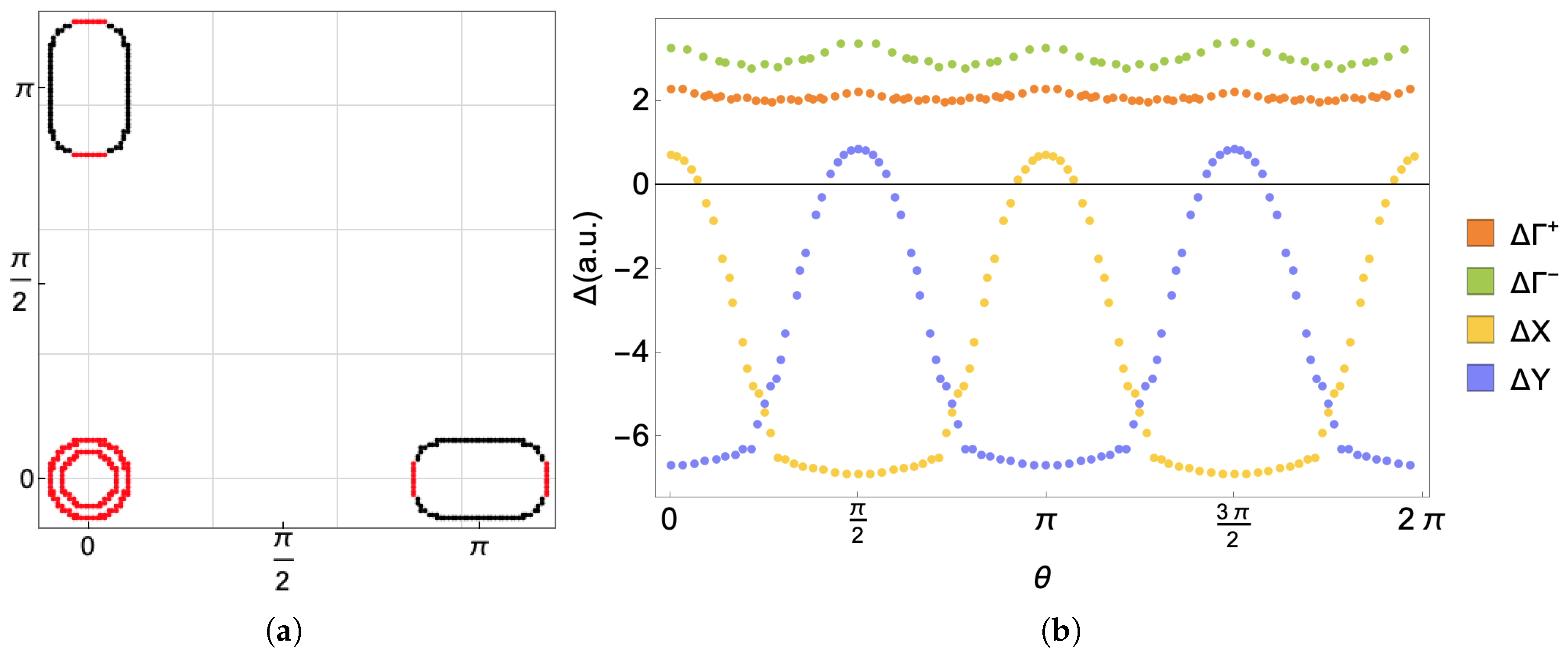
We solved numerically the linearized gap equations by searching for the largest eigenvalue that corresponds to the leading instability of the system. Then, we calculated its corresponding eigenfunction, which determines the symmetry and the structure of the gap function. We found an anisotropic $s_{\pm }$ symmetry as the dominant solution, followed by a nearly degenerate $d_{x^2-y^2}$ state, in agreement with previous multiorbital RPA results [5,9,10,11].

The results for the $s_{\pm }$ gap functions are summarized in Figure 5. Given the simplicity of our treatment, it is easy to verify that the overall momentum dependence of the band gaps directly follows from the momentum dependence of the pairing vertex (i.e., of the spin susceptibility) and the orbital make-up of the Fermi surface. As already mentioned, the key parameter that controls the angular modulation of the gap is the orbital matching between the low-energy states connected by the spin fluctuations that determine the structure of the spin susceptibilities (and thus of the pairing vertex). The orbital degree of freedom is also responsible for the hierarchy of the band gaps. In fact, given a similar condition of band nesting between the two hole pockets and the electrons, one could naively predict similar gaps opening along ${\mathsf{\Gamma }}_{\pm }$. However, from Figure 5b, it can be seen that the gap in ${\mathsf{\Gamma }}_{-}$ is larger than the gap in ${\mathsf{\Gamma }}_{+}$. This is a direct consequence of the orbital composition of the nested pockets: in fact, the exchange of intraorbital spin fluctuations between nested pockets having matching orbital, as ${\mathsf{\Gamma }}_{-}-X/Y$, is stronger than the spin exchange between the pockets presenting orbital mismatch, such as ${\mathsf{\Gamma }}_{+}-X/Y$. This reflects a larger spin susceptibility and SC vertex for the pockets presenting a better degree of orbital matching.

The results we obtained are in agreement with more complete RPA five-orbital model calculations. The main advantage of our derivation is that it gave us a new physical insight on the role of the orbital nesting in controlling the features of the SC gaps. We can compare our results, for example, with the ones obtained in [10], where the anisotropy of the gaps for a five-orbital model was discussed in detail by using RPA calculations for the exchange of spin and charge fluctuations. The authors concluded that the anisotropy of the gap on the different Fermi surface pockets arose from the interplay of the orbital make-up of the states on the Fermi surface together with the momentum dependence of the fluctuation exchange pairing interaction. In addition, to minimize the repulsion between the electron pockets, the gap can present accidental nodes. By comparing the results obtained within the OSSF model (Figure 5) and the five-orbital calculation (Figure 4b in [10]), one can see that the OSSF calculations qualitatively reproduce the main feature of the multiorbital ones, i.e., the modulated $s_{\pm }$ symmetry for the gap, with accidental nodes. We also reproduce the correct hierarchy of the band gaps with $|{\Delta }_{\mathbf{k}}^{{\mathsf{\Gamma }}_{-}}|>|{\Delta }_{\mathbf{k}}^{{\mathsf{\Gamma }}_{+}}|$. The main novelty here is that our analysis allows for a straightforward interpretation of the gap anisotropy and the band gap hierarchy in terms of the degree of orbital matching between nested Fermi surfaces.

4. Discussion

In this work, we showed that the OSSF model provides a reliable description of the magnetic excitations in IBSs and represents the minimal model to study spin-mediated superconductivity in this system.

We computed the spin susceptibility for a four-pocket model in the tetragonal phase and compared the results with the ones obtained for the five-orbital model. Depending on the degree of orbital nesting between pockets, we obtained an orbital modulation of the spin susceptibility that gives rise to commensurate or incommensurate peaks in the spin susceptibility when there is an orbital match or mismatch between the hole and the electron pockets, respectively. The spin exchange between pockets with matching orbitals is the larger contribution to the total spin susceptibility. By comparing the total spin susceptibility of the OSSF model with the one obtained within the five-orbital model, we showed that the OSSF reproduces qualitatively well the overall momentum dependence and the relative heights and widths of the peaks located at different momenta. This is a remarkable result considering that the OSSF model is a low-energy effective model that only considers the $yz,xz,xy$ orbitals and that the OSSF reduces the computation of the spin susceptibility to a few intraorbital scalar components.

We computed the pairing vertex mediated by the OSSF and the corresponding gap equations. Due to the intraorbital scalar character of the spin susceptibility of the OSFF model, it is possible to draw analytically the Feynman diagrams involved in the pairing vertex, something that is almost unfeasible within the five-orbital model due to the large number of different possible diagrams. By solving the corresponding BCS equations, we found as a leading instability a $s_{\pm }$ symmetry and a nearly degenerate $d_{x^2-y^2}$, in agreement with multiorbital calculations. Our finding of a close competition between the $s_{\pm }$ ground state and the $d_{x^2-y^2}$ appears in agreement with Raman experiments in various IBSs [30,31,32,33,34,35]. The analysis of the subdominant $d_{x^2-y^2}$ symmetry within the OSSF model is beyond the scope of this work. However, we expect that the inclusion of the orbital degree of freedom within multiband approaches implemented so far (see, e.g., [36,37,38,39,40]) could provide further insight on the SC properties of IBS.

The analysis of the bands gap structure shows that the angular dependence and the magnitudes of the different gaps depend directly on the degree of orbital matching between the hole and the electron pockets. In particular, the orbital nesting between the different Fermi surfaces is the parameter that controls the hierarchy of the band gaps, in contrast with the naive expectation of having a gap proportional to the degree of band nesting. This new insight on the role of the orbital composition of the nested pockets breaks the usual paradigm based on the Fermi surface matching as the parameter controlling the instabilities and establishes the orbital nesting as the crucial control parameter. It is worth noticing that the connection between the gap hierarchy and orbital matching of the nested pockets is more robust than a naive band nesting argument, as it does not depend on the fine-tuned matching of the size and shape of the Fermi surfaces, but relies instead on the orbital composition of the bands determined by the space group of the iron plane of IBSs.

In conclusion, in this work, we analyzed the magnetic excitations and SC gaps for a generic IBS system in the tetragonal phase using the OSSF model. Despite its simplicity, the OSSF model is able to reproduce well all the relevant qualitative features of the spin excitations and pairing interactions of the multiorbital description. It allows for an analytical treatment, making the interpretation of the results straightforward. Due to the orbital selectivity of the spin fluctuation, it allows including in a very simple way additional interacting channels, as we showed explicitly by considering the electron–electron interaction besides the hole–electron spin exchange. The simplified frame of the OSSF allowed us to gain physical insight into the role of orbital nesting in determining the angular modulations and the hierarchy of the band gaps. This result proves that the OSSF model is the minimal low energy model to study spin-mediated superconductivity in IBSs as it correctly incorporates in the low energy description the orbital composition of the bands determined by the space group of the iron plane.

References

- Mazin, I.I.; Singh, D.J.; Johannes, M.D.; Du, M.H. Unconventional Superconductivity with a Sign Reversal in the Order Parameter of LaFeAsO1−xFx. Phys. Rev. Lett. 2008, 101, 057003. [Google Scholar] [CrossRef] [PubMed] [Green Version]
- Kuroki, K.; Onari, S.; Arita, R.; Usui, H.; Tanaka, Y.; Kontani, H.; Aoki, H. Unconventional Pairing Originating from the Disconnected Fermi Surfaces of Superconducting LaFeAsO1−xFx. Phys. Rev. Lett. 2008, 101, 087004. [Google Scholar] [CrossRef] [PubMed] [Green Version]
- Boeri, L.; Dolgov, O.V.; Golubov, A.A. Is LaFeAsO1−xFx an Electron-Phonon Superconductor? Phys. Rev. Lett. 2008, 101, 026403. [Google Scholar] [CrossRef] [PubMed] [Green Version]
- Chubukov, A. Itinerant electron scenario. In Iron-Based Superconductivity; Johnson, P.D., Xu, G., Yin, W.G., Eds.; Springer International Publishing: Cham, Switzerland, 2015. [Google Scholar] [CrossRef]
- Graser, S.; Maier, T.A.; Hirschfeld, P.J.; Scalapino, D.J. Near-degeneracy of several pairing channels in multiorbital models for the Fe pnictides. New J. Phys. 2009, 11, 025016. [Google Scholar] [CrossRef]
- Ikeda, H.; Arita, R.; Kune, J. Phase diagram and gap anisotropy in iron-pnictide superconductors. Phys. Rev. B 2010, 81, 054502. [Google Scholar] [CrossRef] [Green Version]
- Graser, S.; Kemper, A.F.; Maier, T.A.; Cheng, H.P.; Hirschfeld, P.J.; Scalapino, D.J. Spin fluctuations and superconductivity in a three-dimensional tight-binding model for BaFe2As2. Phys. Rev. B 2010, 81, 214503. [Google Scholar] [CrossRef] [Green Version]
- Scalapino, D.J. A common thread: The pairing interaction for unconventional superconductors. Rev. Mod. Phys. 2012, 84, 1383–1417. [Google Scholar] [CrossRef] [Green Version]
- Hirschfeld, P.J.; Korshunov, M.M.; Mazin, I.I. Gap symmetry and structure of Fe-based superconductors. Rep. Prog. Phys. 2011, 74, 124508. [Google Scholar] [CrossRef] [Green Version]
- Maier, T.A.; Graser, S.; Scalapino, D.J.; Hirschfeld, P.J. Origin of gap anisotropy in spin fluctuation models of the iron pnictides. Phys. Rev. B 2009, 79, 224510. [Google Scholar] [CrossRef] [Green Version]
- Hirschfeld, P.J. Using gap symmetry and structure to reveal the pairing mechanism in Fe-based superconductors. Comptes Rendus Phys. 2016, 17, 197–231. [Google Scholar] [CrossRef]
- Sobota, J.A.; He, Y.; Shen, Z.X. Angle-resolved photoemission studies of quantum materials. Rev. Mod. Phys. 2021, 93, 025006. [Google Scholar] [CrossRef]
- Fanfarillo, L.; Cortijo, A.; Valenzuela, B. Spin-orbital interplay and topology in the nematic phase of iron pnictides. Phys. Rev. B 2015, 91, 214515. [Google Scholar] [CrossRef] [Green Version]
- Christensen, M.H.; Kang, J.; Andersen, B.M.; Fernandes, R.M. Spin-driven nematic instability of the multiorbital Hubbard model: Application to iron-based superconductors. Phys. Rev. B 2016, 93, 085136. [Google Scholar] [CrossRef] [Green Version]
- Fanfarillo, L.; Benfatto, L.; Valenzuela, B. Orbital mismatch boosting nematic instability in iron-based superconductors. Phys. Rev. B 2018, 97, 121109. [Google Scholar] [CrossRef] [Green Version]
- Cvetkovic, V.; Vafek, O. Space group symmetry, spin–orbit coupling, and the low-energy effective Hamiltonian for iron-based superconductors. Phys. Rev. B 2013, 88, 134510. [Google Scholar] [CrossRef] [Green Version]
- Kuroki, K.; Usui, H.; Onari, S.; Arita, R.; Aoki, H. Pnictogen height as a possible switch between high-Tc nodeless and low-Tc nodal pairings in the iron-based superconductors. Phys. Rev. B 2009, 79, 224511. [Google Scholar] [CrossRef] [Green Version]
- Kemper, A.F.; Korshunov, M.M.; Devereaux, T.P.; Fry, J.N.; Cheng, H.P.; Hirschfeld, P.J. Anisotropic quasiparticle lifetimes in Fe-based superconductors. Phys. Rev. B 2011, 83, 184516. [Google Scholar] [CrossRef] [Green Version]
- Bascones, E.; Valenzuela, B.; Calderòn, M.J. Magnetic interactions in iron superconductors: A review. Comptes Rendus Phys. 2016, 17, 36–39. [Google Scholar] [CrossRef]
- Ran, Y.; Wang, F.; Zhai, H.; Vishwanath, A.; Lee, D.H. Nodal spin density wave and band topology of the FeAs-based materials. Phys. Rev. B 2009, 79, 014505. [Google Scholar] [CrossRef] [Green Version]
- Fernandes, R.M.; Chubukov, A.V.; Knolle, J.; Eremin, I.; Schmalian, J. Preemptive nematic order, pseudogap, and orbital order in the iron pnictides. Phys. Rev. B 2012, 85, 024534. [Google Scholar] [CrossRef] [Green Version]
- Fanfarillo, L.; Mansart, J.; Toulemonde, P.; Cercellier, H.; Le Fèvre, P.; Bertran, F.; Valenzuela, B.; Benfatto, L.; Brouet, V. Orbital-dependent Fermi surface shrinking as a fingerprint of nematicity in FeSe. Phys. Rev. B 2016, 94, 155138. [Google Scholar] [CrossRef] [Green Version]
- Benfatto, L.; Valenzuela, B.; Fanfarillo, L. Nematic pairing from orbital-selective spin fluctuations in FeSe. NPJ Quantum Mater. 2008, 3, 56. [Google Scholar] [CrossRef] [Green Version]
- Fernández-Martín, R.; Fanfarillo, L.; Benfatto, L.; Valenzuela, B. Anisotropy of the dc conductivity due to orbital-selective spin fluctuations in the nematic phase of iron superconductors. Phys. Rev. B 2019, 99, 155117. [Google Scholar] [CrossRef] [Green Version]
- Altmeyer, M.; Guterding, D.; Hirschfeld, P.J.; Maier, T.A.; Valentí, R.; Scalapino, D.J. Role of vertex corrections in the matrix formulation of the random phase approximation for the multiorbital Hubbard model. Phys. Rev. B 2016, 94, 214515. [Google Scholar] [CrossRef] [Green Version]
- Kemper, A.F.; Maier, T.A.; Graser, S.; Cheng, H.P.; Hirschfeld, P.J.; Scalapino, D.J. Sensitivity of the superconducting state and magnetic susceptibility to key aspects of electronic structure in ferropnictides. New J. Phys. 2010, 12, 073030. [Google Scholar] [CrossRef]
- Grafe, H.J.; Paar, D.; Lang, G.; Curro, N.J.; Behr, G.; Werner, J.; Hamann-Borrero, J.; Hess, C.; Leps, N.; Klingeler, R.; et al. As75 NMR Studies of Superconducting LaFeAsO0.9F0.1. Phys. Rev. Lett. 2008, 101, 047003. [Google Scholar] [CrossRef]
- Fanlong, N.; Kanagasingham, A.; Takashi, I.; Athena, S.S.; Ronying, J.; Michael, A.M.; Brian, C.S.; David, M. Spin Susceptibility, Phase Diagram, and Quantum Criticality in the Eelctron-Doped High Tc Superconductor Ba(Fe1−xCox)2As2. J. Phys. Soc. Jpn. 2009, 78, 4. [Google Scholar] [CrossRef] [Green Version]
- Inosov, D.S.; Park, J.T.; Bourges, P.; Sun, D.L.; Sidis, Y.; Schneidewind, A.; Hradil, K.; Haug, D.; Lin, C.T.; Keimer, B.; et al. Normal-state spin dynamics and temperature-dependent spin-resonance energy in optimally doped BaFe1.85Co0.15As2. Nat. Phys. 2010, 6, 178–181. [Google Scholar] [CrossRef] [Green Version]
- Kretzschmar, F.; Muschler, B.; Böhm, T.; Baum, A.; Hackl, R.; Wen, H.H.; Tsurkan, V.; Deisenhofer, J.; Loidl, A. Raman-Scattering Detection of Nearly Degenerate s-Wave and d-Wave Pairing Channels in Iron-Based Ba0.6K0.4Fe2As2 and Rb0.8Fe1.6Se2 Superconductors. Phys. Rev. Lett. 2013, 110, 187002. [Google Scholar] [CrossRef] [Green Version]
- Böhm, T.; Kemper, A.F.; Moritz, B.; Kretzschmar, F.; Muschler, B.; Eiter, H.M.; Hackl, R.; Devereaux, T.P.; Scalapino, D.J.; Wen, H.H. Balancing Act: Evidence for a Strong Subdominant d-Wave Pairing Channel in Ba0.6K0.4Fe2As2. Phys. Rev. X 2014, 4, 041046. [Google Scholar] [CrossRef]
- Wu, S.F.; Richard, P.; Ding, H.; Wen, H.H.; Tan, G.; Wang, M.; Zhang, C.; Dai, P.; Blumberg, G. Superconductivity and electronic fluctuations in Ba1−xKxFe2As2 studied by Raman scattering. Phys. Rev. B 2017, 95, 085125. [Google Scholar] [CrossRef] [Green Version]
- Böhm, T.; Kretzschmar, F.; Baum, A.; Rehm, M.; Jost, D.; Hosseinian Ahangharnejhad, R.; Thomale, R.; Platt, C.; Maier, T.A.; Hanke, W.; et al. Microscopic origin of Cooper pairing in the iron-based superconductor Ba1−xKxFe2As2. NPJ Quantum Mater. 2018, 3, 48. [Google Scholar] [CrossRef] [Green Version]
- Jost, D.; Scholz, J.R.; Zweck, U.; Meier, W.R.; Böhmer, A.E.; Canfield, P.C.; Lazarević, N.; Hackl, R. Indication of subdominant d-wave interaction in superconducting CaKFe4As4. Phys. Rev. B 2018, 98, 020504. [Google Scholar] [CrossRef] [Green Version]
- He, G.; Li, D.; Jost, D.; Baum, A.; Shen, P.P.; Dong, X.L.; Zhao, Z.X.; Hackl, R. Raman Study of Cooper Pairing Instabilities in (Li1−xFex)OHFeSe. Phys. Rev. Lett. 2020, 125, 217002. [Google Scholar] [CrossRef] [PubMed]
- Maiti, S.; Hirschfeld, P.J. Collective modes in superconductors with competing s- and d-wave interactions. Phys. Rev. B 2015, 92, 094506. [Google Scholar] [CrossRef] [Green Version]
- Maiti, S.; Maier, T.A.; Böhm, T.; Hackl, R.; Hirschfeld, P.J. Probing the Pairing Interaction and Multiple Bardasis-Schrieffer Modes Using Raman Spectroscopy. Phys. Rev. Lett. 2016, 117, 257001. [Google Scholar] [CrossRef] [Green Version]
- Müller, M.A.; Shen, P.; Dzero, M.; Eremin, I. Short-time dynamics in s+is-wave superconductor with incipient bands. Phys. Rev. B 2018, 98, 024522. [Google Scholar] [CrossRef] [Green Version]
- Müller, M.A.; Volkov, P.A.; Paul, I.; Eremin, I.M. Collective modes in pumped unconventional superconductors with competing ground states. Phys. Rev. B 2019, 100, 140501. [Google Scholar] [CrossRef] [Green Version]
- Müller, M.A.; Eremin, I.M. Signatures of Bardasis-Schrieffer mode excitation in Third-Harmonic generated currents. arXiv 2021, arXiv:2107.02834. [Google Scholar]
Figure 1.
Fermi surface for the four-pocket model. The colors represent the main orbital character of the Fermi surface. Notice the orbital nesting between the inner hole pocket and the electron pockets. On the contrary, the Fermi surface of the outer hole pocket presents orbital mismatch with the electron pockets. The green/red arrows denote the orbital selective spin fluctuations (OSSFs), connecting hole and electron pockets at different momenta; see Equations (4)–(6).
Figure 2.
RPA spin susceptibility for a four-pocket model in the tetragonal phase. Three-dimensional maps (upper panels) and two-dimensional cuts (bottom panels) of the RPA susceptibilities shown in the space around the high symmetry points X for the hole–electron sector and M for the electron–electron sector. The orbital composition of the nested bands is at the origin of the momentum dependence of the RPA spin susceptibilities that present commensurate/incommensurate peaks depending on the orbital match/mismatch of the nested Fermi surfaces. The band parameters used in the calculations are detailed in Appendix D; the interaction is fixed at = 1 eV; and the temperature is eV.
Figure 3.
Total RPA spin susceptibility for the four-pocket model. We show the cuts along the high symmetry directions of the RPA spin susceptibility obtained within (a) the OSSF model and (b) the five-orbital model. Temperature is fixed to eV in both panels. We set the effective low-energy interaction as = 1 eV in (a), while the intraorbital and the interorbital on-site interactions for the five-orbital models are set to U = 1.2 eV, U, and in (b). The RPA susceptibility for the five-orbital model is computed for any momentum as it follows from a full-band calculation. On the other hand, the OSSF model is a low energy model, thus providing information of the bands at the Fermi level (Fermi pockets) only. This implies that not all possible values of are allowed. The RPA susceptibility is this case is well defined around the high symmetry points only, as one can see in Panel (a). Nonetheless, we find a remarkable qualitative agreement within the low-energy calculation and the five-orbital one.
Figure 4.
Pairing vertex in the random phase approximation up to fourth-order within the OSSF model.
Figure 5.
RPA gap functions within the OSSF model (a) plotted on the Fermi surface pockets (red circles for positive and black circles for negative gaps) and (b) plotted as a function of the angle from 0 to . The SC gap functions present symmetry with angular modulations controlled by the orbital composition of the nested bands. The hierarchy of the band gaps follows from the orbital nesting properties of the matching Fermi surface pockets. Band parameters are detailed in Appendix D, eV.
Publisher’s Note: MDPI stays neutral with regard to jurisdictional claims in published maps and institutional affiliations. |
© 2021 by the authors. Licensee MDPI, Basel, Switzerland. This article is an open access article distributed under the terms and conditions of the Creative Commons Attribution (CC BY) license (https://creativecommons.org/licenses/by/4.0/).
Share and Cite
MDPI and ACS Style
Fernández-Martín, R.; Calderón, M.J.; Fanfarillo, L.; Valenzuela, B. The Role of Orbital Nesting in the Superconductivity of Iron-Based Superconductors. Condens. Matter 2021, 6, 34. https://doi.org/10.3390/condmat6030034
AMA Style
Fernández-Martín R, Calderón MJ, Fanfarillo L, Valenzuela B. The Role of Orbital Nesting in the Superconductivity of Iron-Based Superconductors. Condensed Matter. 2021; 6(3):34. https://doi.org/10.3390/condmat6030034
Chicago/Turabian StyleFernández-Martín, Raquel, María J. Calderón, Laura Fanfarillo, and Belén Valenzuela. 2021. "The Role of Orbital Nesting in the Superconductivity of Iron-Based Superconductors" Condensed Matter 6, no. 3: 34. https://doi.org/10.3390/condmat6030034