The Maximum Common Subgraph Problem: A Parallel and Multi-Engine Approach


1
Dipartimento di Automatica e Informatica, Politecnico di Torino, Corso Duca degli Abruzzi 24, 10129 Torino, Italy
2
Cisco Systems, Talos Security Intelligence and Research Group, 06250 Sophia Antipolis, France
*
Author to whom correspondence should be addressed.
Computation 2020, 8(2), 48; https://doi.org/10.3390/computation8020048
Submission received: 8 April 2020
/
Revised: 6 May 2020
/
Accepted: 13 May 2020
/
Published: 18 May 2020
(This article belongs to the Section Computational Engineering)
Abstract
:The maximum common subgraph of two graphs is the largest possible common subgraph, i.e., the common subgraph with as many vertices as possible. Even if this problem is very challenging, as it has been long proven NP-hard, its countless practical applications still motivates searching for exact solutions. This work discusses the possibility to extend an existing, very effective branch-and-bound procedure on parallel multi-core and many-core architectures. We analyze a parallel multi-core implementation that exploits a divide-and-conquer approach based on a thread pool, which does not deteriorate the original algorithmic efficiency and it minimizes data structure repetitions. We also extend the original algorithm to parallel many-core GPU architectures adopting the CUDA programming framework, and we show how to handle the heavily workload-unbalance and the massive data dependency. Then, we suggest new heuristics to reorder the adjacency matrix, to deal with “dead-ends”, and to randomize the search with automatic restarts. These heuristics can achieve significant speed-ups on specific instances, even if they may not be competitive with the original strategy on average. Finally, we propose a portfolio approach, which integrates all the different local search algorithms as component tools; such portfolio, rather than choosing the best tool for a given instance up-front, takes the decision on-line. The proposed approach drastically limits memory bandwidth constraints and avoids other typical portfolio fragility as CPU and GPU versions often show a complementary efficiency and run on separated platforms. Experimental results support the claims and motivate further research to better exploit GPUs in embedded task-intensive and multi-engine parallel applications.
1. Introduction
Graphs are an extremely general and powerful data structure.
They can be used to model, analyze, and process a huge variety of phenomena and concepts by providing natural machine-readable representations. For instance, graphs may be used to represent the relationships between functions or fragments of code in programs, or the connections among functional blocks in electronic circuits.
Given a graph G, a graph H is a subgraph of G if all its vertices are also vertices of G. The subgraph H is called induced if it includes all the edges of G between its vertices; it is called non-induced, or partial, otherwise. The maximum common subgraph problem consists in finding the largest graph which is simultaneously isomorphic to a subgraph of two given graphs. The problem comes in two forms, namely the maximum common induced and the maximum common partial (or maximum common edge) subgraph problem. In the former, the goal is to find a graph with as many vertices as possible which is an induced subgraph of each of the two input graphs, that is, edges are mapped to edges and non-edges to non-edges. In the latter, the target is to find a common non-induced subgraph, that is, a graph with as many edges as possible. In this case “partial” indicates that not all edges need to be mapped, i.e., some edges might be skipped. In this paper, we discuss the induced variant, and for the sake of simplicity we will refer to it simply as the maximum common subgraph problem (MCS).
MCS problems arise in many areas, such as bioinformatics, computer vision, code analysis, compilers, model checking, pattern recognition, and have been discussed in literature since the seventies [1,2]. MCS has been recognized as an NP-hard problem and it is computationally challenging in the general case. In practice, running state-of-the-art algorithms become computationally unfeasible on problems with as little as 40 vertices, unless some meta information allows to reduce the search space. Practitioners from many fields are still asking researchers how to effectively tackle the problem in their real-world applications.
In 2017 McCreesh et al. [3] proposed McSplit, a very efficient branch-and-bound algorithm to find maximum common subgraphs for a large variety of graphs, such as undirected, directed, labeled with several labeling strategies, etc. Essentially, McSplit is a recursive procedure adopting a smart invariant and an effective bound prediction formula. The invariant considers a new vertex pair, within the current mapping between the two graphs, only if the vertices within the pair share the same label, i.e., they are connected in the same way to all previously selected vertices. The bound consists in computing, from the current mapping size and from the labels of yet to map vertices, the maximum MCS size the current recursion path may lead to, and to prune those paths that are not promising enough.
Within this framework, this paper presents the following contributions:
- As sequential programming has often become “parallel programming” [4,5], we present a CPU-based multi-core parallel design of the McSplit procedure. In this application, we parallelize the searching procedure viewing the backtrack search as forming a tree, and exploring different portions of the tree using different threads. Although high-level architecture-independent models (such as Thread Building Block, OpenMP, and Cilk) enable easy integration into existing applications, native threading approaches allow much more control over exactly what happens on what thread. For that reason, we adopt a native threading programming model to develop our CPU-based application, where threads are organized in a thread pool. The pool shares a queue in which tasks are inserted by a “master” thread and later extracted and solved by the first free “helper” thread. Mechanisms are used to avoid task duplication, task unbalance, and data structure repetition, as such problems may impair the original divide-and-conquer approach. A compact data structure, which represents partial results, is used to share solutions among threads.
- As in the last few years, it has become pretty clear that programming General Purpose GPU (GPGPU) applications is a move in the right direction for all professional users [6,7], we analyze how to extend the previous approach to many-core GPGPUs. First, we describe how to transform an intrinsically recursive solution into an iterative one which is able to handle the heavy workload unbalance and the massive data dependency of the original, recursive algorithm. After that, we select the implementation framework and redesign the parallel application. Nowadays, CUDA and OpenCL are the leading GPGPU frameworks, and each one brings its own advantages and disadvantages. CUDA is a proprietary framework created by NVIDIA, whilst OpenCL is open source. Even if OpenCL is supported in more applications than CUDA, the general consensus is that CUDA generates better performance results as NVIDIA provides extremely good integration. For that reason, we describe the corrections required to the multi-core CPU-based algorithm to handle the heavy workload unbalance and the massive data dependency of the original recursive algorithm on the CUDA framework. We would like to emphasize here that our implementation works only on NVIDIA GPUs, even if an OpenCL implementation would imply moderate modifications and corrections.
- As the MCS problem implicitly imply poor scalability, we present a few heuristics to modify the original procedure on hard-to-solve instances. The first one modifies the initial ordering used by the branch-and-bound procedure to pair vertices and to generate the recursion tree. Moreover, we suggest counter-measures to deal with the “heavy-tail phenomenon”, i.e., the condition in which no larger MCS is found, but the branch-and-bound procedure keeps recurring. Finally, following other application fields (such as the one of SATisfiability solvers [8]), we propose randomize tree search and automatic search restarts for expensive computations. These heuristics show very good performance on specific instances even if they cannot outperform the original implementation on average.
- To leverage the advantages and disadvantages of the various strategies we implemented, we extend the classical “winner-takes-all” approach to the MCS problem to a multi-engine (portfolio) methodology [8,9,10]. In our approach, different implementations may resort to different computation units, namely CPU and GPU cores, with a corresponding increase of both the overall memory bandwidth and the computational power and a consequent reduction of the classical multi-engine fragilities.
We run experiments on standard benchmarks coming from [11,12]. We compare the original McSplit implementations against the many-core, the multi-core, and the portfolio implementation. We also consider some intermediate versions, generated to move from the multi-core to the many-core and to the multi-engine approach, and we specify the advantages and disadvantages of each of them.
To sum up, we believe contributions 2, 3, and 4 do appear for the first time for the presented application. Contribution 1 can be considered as an extension of previous works, which uses a slightly different multi-threading approach and a different implementation language. It is also an intermediate step towards contribution 2. The impact of these contributions is proved by our experiments which compare our implementations with state-of-the-art tools on standard benchmarks.
Roadmap
The paper is organized as follow. Section 2 reports some background on graph isomorphism, and it summarizes McSplit. Section 3.1, Section 3.2, and Section 4 introduce our parallel multi-core, many-core, and multi-engine (portfolio) implementations, respectively. Section 5 reports our evidence analysis. Finally, Section 6 includes some final considerations and Section 7 presents a few possible main paths for further developments.
2. Background and Related Works
2.1. The Maximum Common Subgraph Problem
Finding the similarity of two graphs has been the subject of extensive research in the last decades [3,13,14,15,16,17,18,19,20]. Given a graph , a graph is a subgraph of graph G (i.e., ) if it is composed by a set of vertices such that . If H includes all the edges with both the endpoints in , it is called an induced subgraph. Otherwise, H is called a non-induced or partial subgraph. In this work, we will consider only induced subgraphs.
Figure 1 shows some examples of induced and of non-induced subgraphs. Given two graphs, G and H, the graph S is a common subgraph if S is simultaneously isomorphic to a subgraph of G and to a subgraph of H.
An MCS of G and H is the largest possible common induced subgraph, i.e., the common subgraph with as many vertices as possible. Figure 2 shows some examples with undirected and unlabeled graphs.
In the rest of the paper, we will indicate with and the number of vertices of G and H, respectively.
2.2. Related Works
MCS problems are common in biology and chemistry, in computer vision, computer-aided manufacturing, malware detection and program analysis, crisis management, and in social network analysis. The MCS problem is also strictly related to others classical graph algorithms such as finding a maximum common subgraph between two graphs. This in turn is the key step to measure the similarity or difference between two graphs [21,22]. As a consequence, several approaches have been adopted to solve MCS problems over the last a few years.
2.2.1. Sequential Approaches
McGregor [23] proposes a branch-and-bound algorithm based on two basic features. He first builds a searching tree in which the match between two vertices corresponds to a branch. Then, he constrains the search with a bounding function which evaluates the number of vertices that may still be matched. In this way, the current searching branch is pruned as soon as the bound becomes lower than the size of the largest known common subgraph. Many recent Constraint Programming (CP) approaches may be viewed as enhancements of this procedure.
Vismara et al. [15] introduce the first explicit CP model. Given two graphs G and H, constraint programming associates to every vertex a variable whose domain ranges over each vertex in H, plus an additional value which is used when the vertex v is not matched to any vertex of H. Edge constraints are introduced in order to ensure that variable assignments preserve edges and non-edges between matched vertices. Difference constraints are introduced in order to ensure that each vertex of H is assigned to at most one variable. Once these assumptions are given, the objective is simply to find an assignment of values to the variables v, maximizing the number of variables matched with a vertex in H.
This CP model was later improved by Ndiaye and Solnon [24] by replacing binary difference constraints with a soft global constraint. This constraint maximizes the number of vertices from G and H that are matched, while ensuring that each vertex of G is matched with a different vertex of H.
A completely different solution strategy is based on the concepts of association graph [25,26] and maximum clique. Given two graphs G and H, their association graph is a graph which includes a vertex for each matching pair composed by a node of G and a node of H, and all edges between them. It can be proved that a clique in an association graph corresponds to a set of compatible vertex mates. Therefore, the method proceeds in two steps. During the first one, the association graph of G and H is built. During the second one, the maximum clique of the association graph is found, delivering the desired MCS. When combined with a state-of-the-art maximum clique solver, this strategy is one of the best approaches for solving the problem on labeled graphs [27]. However, the association graph encoding is extremely memory-intensive, limiting its practical use to pairs of graphs with no more than a few hundred vertices.
Piva et al. [28] solve the induced version of the MCS problem with an algorithm based on Integer Programming (IP) and polyhedral combinatorics techniques. Essentially, the authors build a better formulation of the problem as an IP by theoretically investigating it using the polyhedral theory. Then, they verify the impact of these theoretical results in the computational performance of Branch-and-Bound and Branch-and-Cut algorithms.
Englert et al. [29] focus on the MCS problem applied to molecular graphs. The authors propose several heuristics to improve the accuracy and efficiency of previous algorithms as well as to increase the chemical relevance of their results. Among the suggested heuristics, the authors use extended connectivity fingerprints to search for MCSs and they provide a chemically relevant atom mapping.
Hoffman et al. [30] approach the MCS problem via the subgraph isomorphism problem. The subgraph isomorphism problem consists in finding a copy of a small pattern graph inside a larger target graph. In general, this is much less computationally challenging than the MCS problem. Anyhow, the authors propose the k↓ algorithm which tries to solve the subgraph isomorphism problem for , i.e., in the case in which the whole pattern graph can be found in the target. Should that not be satisfiable, k↓ tries to solve the problem for , i.e., with one vertex non matched, and should that also not be satisfiable, it iteratively increases k until the result is satisfiable. k↓ exploits strong invariants using paths and the degrees of vertices to prune large portions of the search space. Moreover, it mainly targets large instances, where the two graphs are of different orders but it is expected that the solution will involve most of the smaller graph.
2.2.2. Parallel Approaches
Several parallel methods concentrate on how to solve the subgraph isomorphism problem. McCreesh and Prosser [31] focus on constraint programming. The authors firstly introduce the concept of “supplemental” graph. Then, they use a weaker inference than previous CP strategies and they describe a variation of conflict-directed backjumping. After that, they suggest a thread-parallel implementation of the pre-processing and of the search phases. Finally, they explain how parallel search may safely interact with backjumping. Archibald et al. [32] designed an algorithm for subgraph isomorphism that instead of using the degree of a vertex to sort the matching pairs, adopts it to direct the proportion of search effort spent in different subproblems. This increases parallelization, such that the authors get impressive speedup on both satisfiable and unsatisfiable instances.
MCS problems are the target of Minot et al. [33], who describe a structural decomposition method for constraint programming. Their decomposition generates independent subproblems, which can then be solved in parallel. The authors compare their structural decomposition with domain-based decompositions, which basically split variable domains. They finally proved that the new method leads to better speedups in some classes of instances. McCreesh [34] presents parallel algorithms for the maximum clique and the subgraph problem, whereas he just reports some considerations for the parallel MCS problem. Following this work, Hoffmann et al. [35] compare the sequential and the parallel versions of three state-of-the art branch and bound algorithms for the MCS problem. Even if the authors prove that the parallel version of each algorithm is better than the corresponding sequential version, they mainly focus on presenting and interpreting the experimental data, rather than describing implementation details.
Other works concentrate on similar but different problems. For example, Kimming et al. [36] study the subgraph enumeration problem, in which the target is to find all subgraphs of a target graph that are isomorphic to a given pattern graph. The authors present a shared-memory parallelization of a state-of-the-art subgraph enumeration algorithms based on work stealing. Their implementation demonstrates a significant speedup on real-world biochemical data, despite a highly irregular data access pattern. The maximum clique problem is the subject of McCreesh et al. [37]. In this work, the authors concentrate on multi-core thread-parallel variants of a state-of-the-art branch-and-bound algorithm. They firstly analyze a few parallel strategies to demonstrate why some implementation choices give better or worse performance on some problems. Then, they present a new splitting mechanism which explicitly diversifies the search on top and that later re-splits work to improve balance. The authors show that their splitting strategy gives better and more consistent speedups than other mechanisms.
2.3. The McSplit Algorithm
In 2017, McCreesh et al. [3] proposed McSplit, a very effective branch-and-bound procedure to find MCSs. McSplit is essentially a recursive procedure based on two main ingredients: a smart invariant and an effective bound prediction formula. Different implementations of the algorithm have been provided by the authors.
The procedure dovetails the two ingredients in the following way. Let us suppose we have the two graphs G and H represented in Figure 3a,b. We consider graphs as simple as possible for the sake of readability. For now, we also suppose these graphs are undirected (even if they are represented as directed in Figure 3) and unlabeled, i.e., the nodes labels are reported only to uniquely identify all vertices.
McSplit builds a mapping M between the vertices of G and of H using a depth-first search. Initially, M is an empty set, and the algorithm adds a vertex pair to M at each recursion level. During the first recursion step, let us suppose we arbitrarily select vertex a in G, and we try to map this vertex with vertex b in H, that is . Now we label each unmatched vertex in G according to whether it is adjacent to vertex a, and we label each unmatched vertex in H according to whether it is adjacent to vertex b. For undirected graphs, adjacent vertices have label 1 and non-adjacent vertices have label 0. Table 1a shows these labels. At this point, we recur and we try to extend M with a new pair. A new pair can be inserted into M only if the vertices within the pair share the same label. This is McSplit main invariant. If during the second recursion step, we extend M with pair b and c, we obtain the new mapping , and the new label set represented in Table 1b. The third step consists of extending M with c and a, which is, at this point, the only remaining possibility. We obtain and the label set of Table 1c. The last two vertex d and d cannot be inserted int M because they have different labels. Then the recursive procedure backtracks and it looks-for another (possibly longer) match M. After all possibilities have been exhaustively explored, the final result, i.e., the MCS of G and H is represented in Figure 3c.
As previously mentioned, the second very important ingredient of the algorithm is the bound computation. This computation is used to effectively prune the space search. While parsing a branch by means of a recursive call, the following bound is evaluated:
where is the cardinality of the current mapping and L is the actual set of labels. If the bound is smaller than the size of the current mapping, there is no reason to follow that path, as it is not possible to find a matching set longer than the current one along it. In this way the algorithm prunes consistent branches of the decision tree, drastically reducing the computation effort.
As the MCS problem comes in many variants, McCreesh et al. propose small algorithmic variations to deal optimally with directed, vertex-labeled and edge-labeled graphs. For example, if we consider the graph in Figure 3a,b as directed and with node labels, and we apply the previous process incrementing it with the two previous modifications, we find the MCS reported in Figure 3d.
3. Parallel Approaches
In this section, we present our parallel approaches, the CPU-based multi-core in Section 3.1, and the GPU-based many-core in Section 3.2.
3.1. The CPU Multi-Core Approach
While other authors [34,35,38] briefly discuss a parallel multi-thread version to efficiently parallelize the algorithm analyzed in Section 2.3, no complete description of the concurrent MCS function is available in the literature. To have a complete control over threads, we avoid using high-level parallel programming APIs such as Threading Building Block (TBB), OpenMP, or Cilk Plus. Thus, to implement our concurrent version of the algorithm, we decomposed and restructured the original recursive procedure McSplit to balance the workload among native threads. The core procedure delegates to a set of helper threads portions of the job done by the original function during its deeper recursion levels (Figure 4).
The top-level function solve orchestrates all worker threads. It initializes the matching process among vertices, and in order to achieve independence between working threads, it performs a copy of all relevant data structures, before moving into recursion. Depending on the recursion level, function solve goes on calling master threads or helper threads. Helper threads are called at lower recursion levels to help master threads to solve their current tasks. It must be remarked that a master thread is not the first thread started by the operating system and that in different phases of the algorithm, any thread can act as a master thread. Each thread executing the main function of a particular branch of the recursion, and eventually asking for help, acts as a master thread. At the same time, each thread helping a master thread acts as a helper thread. The reason to adopt this strategy is that the concurrency level has been tuned to avoid useless copy of the current solution and to prevent overloading the task queue in the thread-pool with tasks that are too short. Generally speaking, during the first few levels of the recursion, each iteration of the main loop that pairs vertices from the two graphs is very time consuming. On the contrary, the deeper the procedure goes into the recursion tree, the shorter becomes each branch and its associated task. As a consequence, we define a threshold for the maximum depth in the recursion tree above which the function stops delegating work to other threads. Only master threads are called after this threshold, that is, delegation is not used when splitting the current task among more threads is too expensive and it would probably generate too many very short working threads.
In this scenario, threads cooperate with each other to compute, in parallel, different iterations of the main cycle in which pair of vertices are coupled depending on their labels. Thus the main task of all master threads and helper threads is to go on suggesting new matching pairs and eventually recurring on their own recursion path. The main difference between master and helper threads is that the latter make a copy of all incoming data structure before moving on. The main and the helper functions are designed such that they are data-independent, and they can be assigned to different threads to be run in parallel. Anyway, they are actually linked by two atomic variables. The first one is used as a shared index of the main iterative construct. In this way, the master and the helper thread can execute the same cycle, but they must distribute iterations without both executing the same ones. The second atomic variable is the size of the current matching, which is shared among all threads to correctly evaluate the opportunity to proceed along a new path. To be thread-safe, we manipulate these atomic objects using only atomic operators. We use the ones introduced by C11 (i.e., atomic_load, atomic_store, etc.) whose declarations can be found in the header stdatomic.h.
To further increase efficiency, we keep all threads running during the entire execution of the algorithm, and we orchestrate them using a thread pool. Such a pool implements a priority queue in which threads can insert the tasks they want to be helped with. These tasks include copies of the data structures and a pointer to the helper function. Helper threads can pick-up new tasks from the queue as soon as they are available. To achieve a higher level of parallelism, more than one helper thread can pick the same task and cooperate to solve it, also if at different times. The task objects are put in the queue following the order given by their position in the recursion tree. For example, a task generated at depth d will be put in the queue before any tasks generated at depth . In the same way, a task generated at depth d in the iteration of the main loop will be put after a task generated at depth d in the first iteration . The shared variables avoid repeating the same tasks more than once. Within the thread-pool, synchronization and communication among threads is guaranteed adopting a condition variables used, as usual, in conjunction with a mutex. Both the C11 and the POSIX versions of the conditional variable primitives have been tested.
A simplified version of this entire process is represented by Algorithm 1. The top level procedure parallelMCS receives the original graphs G and H as parameters. Lines 1–3 are dedicated to the initialization phase. In line 1, based on the initial labels, we partition the vertices of G and H into classes, storing the resulting partitions into the array . Then, in line 2, we set the current mapping M, and the best mapping , to the empty set. Line 3 is used to allocate the priority queue Q used by the thread-pool, and to initialize all threads working on the queue. After that, we call function solve which is the core branch-and-bound recursive procedure. It essentially adopts the concurrent scheme previously described.
| Algorithm 1 The multi-core CPU-based recursive branch-and-bound MCS procedure. |
parallelMCS (G, H)
solve (, M, , )
|
solve receives as parameters the bidomain partition, the current and the best mapping M and , and the recursion level depth (properly initialized to 0). At each run of the recursive function, if a greater mapping has been found (line 6), the best incumbent graph is updated. Then, the upper bound for the current search branch is computed (line 7) using Equation (1). If the bound has been hit (i.e., the current bound is lower or equal to the size of the actual incumbent, thus no future search on the current path can improve it), the branch is pruned and the function returns (line 8). Otherwise, a new mapping between unmapped vertices is searched. In this case, firstly the most promising label class is selected from the bidomain partition (line 9), according to some heuristic. Then, a vertex belonging to that label class is chosen as a new vertex v (line 10). Finally, the iterative cycle of lines 11–20 visits every vertex u of H belonging to the previously selected label class . For each of these vertices, the recursive function explores the consequences to add the pair , to the mapping M (line 12). Notice that considering as a new pair in the mapping, implies splitting the current classes, stored in , into two new sub-classes, according to whether vertices belonging to it are adjacent or not to v and u. This operation is performed by function filterDomain at line 13. At this point, as previously described, we resort to helper threads for the lower recursion levels (lines 15–16) and we proceed independently for higher depths (line 18). In the first case, a new pool task is first generated (line 15) and then enqueued in the thread pool queue (line 16). In the second case, a new recursive call is performed with the updated label classes , the current mapping M, the best one , and the recursion depth increased by 1 (line 18). Notice that the process reported in lines 14–19 is repeated in lines 22–27. This last section of the code is required to check the case in which the vertex is not mapped at all with any vertex of H. Thus v is ruled-out from the current set of classes (line 21) and the process proceeds either concurrently (lines 23–24) or recursively (line 26).
As a last comment, notice that a fundamental role in the system is played by the queue (Q) within the thread pool and by the working threads running for the entire process and waiting for new tasks () in the queue. In fact, the thread pool guarantees a very balanced work-load among threads: Any time a thread finishes a branch, it can go through the tasks queue and start helping other threads with their branches, thus reducing its idle time. This mechanism, which is not illustrated by the pseudo-code for the sake of simplicity, implies various execution flows, depending on the status of the queue:
- When the program starts and the thread pool is first initialized (line 3), each thread will start its own cycle when the task queue is empty. In this situation each thread acquires the lock on the queue (not everyone at the same time, of course), and then it tries to pick a task from the queue. Since the latter is empty, the thread skips all operations without doing anything, and the thread blocks on the condition variable waiting for someone to put a task in the queue and wake it up (POSIX mutex and condition variable objects are used but not detailed in this description).
- Every time the solve function adds a task to the queue (lines 18 or 26), each thread of the thread pool that in that moment is waiting for the condition variable to become signaled is released. The first thread which manages to acquire the lock proceeds within its main cycle, and it picks the task from the queue. Even if this task should no longer be executed by any other thread, the only entity allowed to remove it from the queue is the one that put it in the queue.
- When the task queue is not empty, tasks are ordered such that they are executed and completed following the order of the recursion. Any completed task that is still being executed by some thread, will be at the beginning of the queue. When a task is executed, it is marked as running, i.e., it has a NULL pointer instead of the actual pointer to the function used to solve the problem. Running tasks are simply skipped by any thread scanning the queue searching for a task to execute. When a task with a non-NULL pointer is found, the execution continues as the previous item point. If no task is found, the execution continues as in the first point.
3.2. The GPU Many-Core Approach
In this section, we show how the algorithm described in Section 3.1 can be modified in order to make it suitable to run on many-core GPUs. Although both CUDA and OpenCL have been the leading GPGPU frameworks in the last decade, CUDA is supposed to generate better performance results. As performance gain is one of the main target of our extension, we decided to use CUDA as developing platform. In the sequel, we will concentrate on the most effective strategies and optimizations among the several different ones that have been implemented in this platform.
As shown in previous sections, McSplit is intrinsically recursive, and its maximum recursion depth is equal to the number of vertices belonging to the final MCS. Unfortunately, even using dynamic parallelism, CUDA does not support more than 24 in-depth recursion levels, and it is then suitable only for graphs with a maximum of 24 nodes. For this reason, the first compulsory step to adapt our algorithm to CUDA is to modify the execution structure in order to formally remove recursion.
Recursion can usually be avoided using an explicit stack. In Algorithm 1 a new recursive call is performed at lines 18 and 26. To avoid these recursive calls, we could substitute these lines as follows. At line 18, we wrap all arguments of the solve procedure in a data structure and we push this structure into a stack. Then, after line 20, we perform an extra iterative construct which pops one item from the stack at every iteration, and it runs a new instance of the solve function with such an argument. This approach, besides not being very sophisticated, remains practically unfeasible on GPUs. Unlike standard recursion, it would use a lot of memory as the stack would store every argument for each virtual recursion of the original for loop at line 11–20. Unfortunately, the quantity of memory for each GPU thread is quite limited. Moreover, as each stack frame would correspond to a branch of the searching tree with a specific tree depth, this approach would lead to an extremely unbalanced workload for the GPU threads as workload will vary with the recursion depth. As a consequence, our main target is to refine this approach to keep under control the memory usage and to increase the work-balance among threads.
3.2.1. Labels Re-Computation
A first attempt to drastically reduce the amount of information stored into the stack, is the following one. Instead of storing all arguments of the solve function in all stack frames as previously suggested, each new stack entry can simply consist in a matching pair, i.e., a pair of integer values representing a possible mapping between a vertex of the first and a vertex of the second graph. Pairs can be pushed to be analyzed in the future, and popped by the thread which is going to analyze them. The first problem with this approach is to synchronize push and pop operations on the stack with the length of the current solution M. If we suppose to store the length of M into a proper variable, we can indicate increments and decrements of its value by storing two different reserved entries in the stack. For example, the value could be used to increase the solution length, and could be used to decrease it.
For example, let us suppose we are searching the MCS of two graphs (G and H) with 5 vertices. Figure 5 sketches the stack storing all pairs still to be managed and the current matching M. At the very beginning, any combination of one vertex from the first graph and one from the second graph is possible, therefore the stack will contain all vertex pairs. To maintain the same processing order of the standard recursive function, pairs can be pushed in the stack in reverse order, i.e., from down to , so that they are later popped in the correct one. When we pop the first pair, namely , we insert this pair into the current solution M, and we also compute the new label classes for each remaining vertex of both the input graphs. Then, we must push in the stack all pairs with matching labels and we move to the second matching pair in the current solution M. To synchronize these operations, we push the reserved entry (the red pair in Figure 5) before pushing all new vertex pairs onto the stack, and we insert the pair (the blue one, in the same figure) after pushing them. In this way, when the pair is popped, we know that the current solution has one more entry, and the position in array M of Figure 5 must be increased from 0 to 1. Similarly, when the pair is extracted, the current solution length has to be decremented to return to zero. In any case, similarly to the standard algorithm, every time a better solution is found, we store it as a new better solution .
Albeit computationally neat and efficient, this stack implementation is unfeasible, because the stack would need to store all possible combination of vertex pairs that we could chose as first pair. The number of such pairs is given by the multiplication principle and it is equal to the product of the degrees of the two input graphs. In other words, the necessity to store separately each vertex pair belonging to the same label class, instead of grouping them into a bidomain which is able to contain all of them, leads to stack whose size is quickly increasing. Moreover, this solution does not allow an efficiently bound computation. Indeed, to compute the bound with Equation (1) for any new branch, we must re-evaluate the labels for each remaining vertex after each pair has been selected. These two drawbacks lead to massive slowdowns and make questionable its utilization in order to solve the problem in reasonable time.
3.2.2. New Bidomain Stack
To recover from the drawbacks highlighted in the previous sub-section, we must find a solution which is able to group vertices in label-classes, to keep the stack small enough, and to maintain the algorithm iterative. To reach these targets, we redesign the previous approach to store into the stack bidomains in an optimized form.
First of all, for the sake of simplicity, we use an over-allocated static matrix to represent our stack. In the stack, we store records including 8 integer values. Thus, the stack becomes a matrix-like data structure, with eight columns and a variable number of rows. Each column must be able to store integers representing values up to the degree of the input graphs. To save memory space, we use unsigned characters limiting the graphs size to 254 vertices (as the value 255 is reserved for internal use). In this way, each stack entry is four byte long, as in the previous implementation, in which each entry contained two integer values. Stack entries of eight bytes allow better memory alignment, leading to benefits in terms of memory performance and address computation. Machines able to deal with graphs larger than 254 vertices should also provide much more memory, so the same algorithm could be adjusted to work with unsigned integers. The first five values correspond to the ones included in the original bidomain data structure and they have the same meaning. They indicate the beginning of the corresponding label class for G, and H (namely, left and right), the length of these label classes (i.e., the left and the right length), and an indication on whether the class include vertices which are adjacent or not to the previously selected ones. The remaining three columns are used to mimic the recursive process within the iterative one. In fact, as we cannot resort to recursion automatism to reinstate local variables when we backtrack, to restore our procedure to a correct status, we push into the stack three values. The sixth value stores the initial value of the right bidomain length (i.e., right length), the seventh one keeps track of the last right vertex which has been selected, and the last one stores the position in the solution for which the bidomain is “valid”. A bidomain set is valid only during the execution of a specific tree path (i.e., higher levels are handled with new bidomains created by the filterDomain function of Figure 1), but as all bidomains coexist into the same stack, we have to separate them depending on the solution level for which they are valid. Thus, the last value allows us to separate bidomains and to correctly select the best bidomain at each new iteration of the algorithm.
Following the previous scheme, to represent our current solution M, and our best one , we use an over-allocated static matrix including two rows and a variable number of columns of unsigned characters.
3.2.3. Our GPU Implementation
Given the data structure illustrated in Section 3.2.2, the GPU algorithm proceeds as reported in Algorithm 2.
Following the parallel version of Algorithm 1, the main function gpuParallelMCS starts its job initializing the required data objects. The , M, and have the meaning already analyzed in Section 3.1, i.e., they store the label classes, the current mapping, and the best mapping, respectively. Similarly to Section 3.1, Q is the data structure storing the problems (i.e., the vertex partitions) used by the CUDA kernel (i.e., the function kernel) to dispatch working threads (i.e., the function solve). Variable (initialized in line 4) is used to count the generated problems up, so that a new kernel function is run (line 13) only when a sufficient number of sub-problems has been generated (line 12).
After that, within the main cycle of lines 5–22, we extract a new problem from the bidomain array (line 6), and we deal with it in one of the following three ways:
- When the partition cannot lead to a better solution, we ignore it and we prune the corresponding searching path (lines 7–8).
- When it can lead to a larger MCS and it represents a small enough recursion level (line 9), we solved it by eventually running a new CUDA kernel (lines 10–15), A new CUDA kernel is run only when the number of pending sub-problems (or threads, i.e., ) is large enough (line 12). When this happens, we run a new kernel (function Kernel, line 13).
- When we do not rule out the problem and we do not run it within a new CUDA kernel, we solve it locally (lines 17–21). In this case the resolution pattern is similar to the many-core CPU code version. First, we select a vertex from the left bidomain and a vertex from the right bidomain (line 18). Then, we store them in the solution M (line 19) and we eventually update (line 20). Finally, we compute the new bidomain set based on the selected vertices (line 21). However, in the recursive algorithm, the selection of a vertex is performed by swapping it with the one at the end of the domain and by decreasing the bidomain size. In the recursive algorithm, this is possible because when backtracking to higher recursion levels, deep bidomains are destroyed, and the ones at higher levels have not been touched by lower recursions, thus the algorithm can continue with consistent data structures. When recursion is removed, however, we lose this important property, and when we select a vertex from the right bidomain and we decrease its size, the original size must be restored using the original value previously stored as the sixth value of the stack frame as described in Section 3.2.2.
| Algorithm 2 The many-core GPU-based iterative branch-and-bound MCS procedure. |
gpuParalleMCS (G, H)
kernel (Q, M, , )
solve (Q, M, , )
|
Lines 23–25 are used to run one final CUDA kernel to keep into account all subproblems (i.e., threads) still pending. The high-level routine gpuParallelMCS, is followed by the kernel function kernel (lines 26–28). This procedure allocates all required data structures and it moves all necessary data from the CPU to the GPU memory (line 26). After that, it calls the grid of threads solve, including (the number of blocks) blocks, each one with (the number of threads) threads.
The thread function solve somehow imitates the original branch-and-bound recursive procedure while proceeding on a single vertex pair partition. Recursion is substituted by the grid of thread manipulating the same set of problems Q. Each thread firstly extract from the problem set the partition on which it has to work. In our pseudo-code this operation is performed with the queue extraction of line 29, but in reality this operation is performed using the CUDA embedded variables representing the block and thread indices. Then, it proceeds through the main cycle of lines 30–38, where it follows a pattern similar to the one of function gpuParallelMCS. At this level, thread synchronization within the threads belonging to the same block is guaranteed by the synchThreads function (mapped on the CUDA __syncthreads instruction). Moreover, we also use atomic functions such as atomicMax and atomicCAS) to perform read-modify-write atomic operations on the objects storing the length of the current solution.
3.2.4. Complexity and Computational Efficiency
Analytical properties of parallel approximate branch-and-bound algorithms have been rarely studied. The maximum possible speedup of a single program as a results of parallelization is known as Amdahl’s law or its extensions the Gustafson’s Law or the Work-span model. For highly parallelizable problems, a k-fold speed-up should be expected when k processors are used. Unfortunately, “anomalies” of parallel branch-and-bound algorithms using the same search strategy as the corresponding sequential algorithms have long been studied [39,40,41]. These anomalies are due to the fact that the sequential and parallel branch-and-bound algorithms do not always explore the same search space. Simulations have shown that the speedup for these algorithms using k processors can be less than one (“detrimental” anomaly), greater than k (acceleration anomaly), or any value between 1 and k (deceleration anomaly). Malapert et al. [42] also showed that, on embarrassingly parallel search problems, the parallel speedup can be completely uncorrelated to the number of workers, making the results hard to analyze.
In our algorithm, the amount of work depends on how fast the bound converges to its final value thus it is not constant and this implies the possibility to have anomalies. Moreover, in our problem even the work balance is unusually difficult. Practically speaking, if the task we are trying to solve is large enough, then for any sequential algorithm its corresponding parallel algorithm is faster as we will show in the experimental section.
Concerning the GPU algorithm, the CUDA version is significantly slower than any other to start, due to the high computing overhead necessary to initialize the environment. This issue will be better discussed in the experimental result section.
As far as the memory used is concerned, memory grows linearly with the number of threads. Anyhow, this is not currently a problem, due to the limited graph size the approach is able to deal in acceptable times and to the compact data structure adopted.
4. The Portfolio Approach
The so-called “portfolio approaches” have been proposed and adopted in several domains. In such approaches, researchers drop the idea of designing a single, optimal algorithm, and resort to a portfolio of different tools, each one able to tackle specific instances of a given problem. The relationship between the properties of a problem instance and the performance of a tool is typically opaque and difficult to capture. As a consequence, the construction of a portfolio normally involves machine-learning activities.
Portfolio approaches were demonstrated the best approach for model checking and satisfiability in recent competition contexts [8,9,43]. In these scenarios, portfolio approaches have often been used in order to emphasize multi-core CPU exploitation and to encourage multi-threaded solutions [44]. Moreover, portfolio approaches have been proved to be more diversified and less sensitive to model characteristics [45,46,47].
Generally speaking, portfolio tools take as input a distribution of problem instances and a set of tools, and constructs a portfolio, optimizing a given objective function. The function can be related to the mean run-time, percent of instances solved, or score in a competition. In our case, we will focus on the number of instances solved in a specific slotted wall-clock time (The wall-clock time is the difference between the time at which the task finishes and the time at which the task started. It is also known simply as elapsed time). Using wall-clock time instead of process time (both as time limit and for tie-breaking) has the advantage to encourage parallelization. Indeed, the concurrency level of each tool can often be guessed only from experimental data, comparing CPU and wall-clock run times. Furthermore, in our portfolio, we may not only have different solvers possibly running in parallel on the CPU cores but at least one version running on the GPU, thus augmenting the range of variations and affecting different hardware devices, with separate resources. To improve scalability and the performances at least on specific and large-instances, we suggest the following heuristics applied to the original sequential or parallel algorithms.
4.1. Portfolio-Oriented Heuristics
4.1.1. Reordering the Adjacency Matrix
An efficient branch-and-bound procedure requires a good initial ordering to rearrange the recursion tree and improve the convergence speed. Our first heuristic (to which we will refer as to in the sequel) proposes an approach based on the analysis and permutation of the adjacency matrix of the two graphs to produce good recursion trees, which may significantly affect the time and memory requirements of the computation. When ordering an adjacency matrix for graph isomorphism, the rows of the matrix correspond to a permutation of the initial pairing scheme. We assume that the order is top-down. A straightforward analysis suggests that it is advantageous to pair variables with similar support sets. McCreesh et al. [3] always sort the vertices in descending order of degree (or total degree, in the case of directed graphs). Anyhow, as the same authors noticed, some improvements is possible in that direction.
In mathematics, a block matrix is a matrix that can be partitioned into a collection of smaller matrices each one including a block of horizontal and vertical lines. If we consider the adjacency matrix of a directed graph, the presence of more than one connected component in the graph signals the existence of a non-trivial block-diagonal form for the matrix. Identifying the connected components of the graph and then ordering each component individually is desirable. Finding the connected components is linear in the size of the matrix, even for full matrices, and leads to a decomposition of the problem. The overall order for a matrix that has multiple connected components is obtained by concatenating the orders for each component. The sorting of the components is based on the ratio between the number of rows and the number of columns. If the ratio is large, the component goes toward the beginning of the schedule.
Within each component, we order the vertices based on their bit relations. A square matrix is called upper triangular if all the entries below the main diagonal are zeros. Our ordering procedure is roughly based on the algorithm of Hellerman and Rarick [48] to put a matrix in bordered block lower-triangular form. Initially, all non-zero rows and columns of the matrix block form the active submatrix. The procedure then iteratively removes rows and columns from the active block submatrix and assigns them to final positions. It iteratively chooses the column that intersects the maximum number of shortest rows of the active submatrix. Then, it moves that column out of the active block submatrix and immediately to its left. Once the active block submatrix vanishes, the block matrix has been permuted.
4.1.2. Dead-End Recovery and Restart Strategy
As analyzed in Section 2.3, the recursive procedure adopts a quite effective bound prediction formula to constrain the tree search. However, this constraining effect is reduced when the value of the current bound gets closer to the actual one. Moreover, repeated adjustments of the bound may drastically slow-down the procedure, forcing it to visit useless tree sub-sections. For this reason function McSplit was also modified using a top-down strategy (similar to the one adopted by k↓ [30]) by calling the main solve function once per goal size, that is, , , , etc., being G the smaller graph between G and H. This procedure has been proved to beat the original ones in those cases in which the MCS covers nearly all of the smaller graph.
Moving in this direction, Figure 6 shows the cost of procedure (the original sequential version of McSplit) as a function of the size of the computed MCS. For the sake of simplicity, we consider only one representative graph pair with increasing size of the MCS, size varying from 15 to 25. Essentially, the two plots report the number of recursions (Figure 6a) and the wall-clock times (Figure 6b) required to move from one value of the bound to the next one. As we use a logarithmic scale along the y-axis, it is easy to infer that costs drastically increase with the bound, and get quite high close to the final bound value.
Keeping this consideration in mind, we define “dead-ends” as the condition in which no larger MCS is found, but the branch-and-bound procedure keeps recurring. Dead-ends re-computation may prove expensive, and we try to forecast them and to reduce their impact. To predict dead-ends, we rely on a global criterion such as the number of recursions. When this number exceeds a specific threshold without improving the size of the minimum common subgraph, we consider the current sub-tree as leading to a dead-end. Thresholds can be evaluated using absolute values or by taking into consideration the number of recursions that led to the last increment of the bound. Once a dead-end is predicted, we reduce its impact using two different procedures.
The first one (referred as heuristic in the sequel) consists in increasing the bound either by a little value (usually 1) or by doubling it. After varying the bound the procedure may prove that the new bound is till reachable, finding a higher bound, or unreachable, proving unable to find a higher bound. In the first case, we have just avoided several useless iterations, pruning the search tree much faster and increasing the convergence speed. In the second one, we have found an upper bound for the size of the MCS. In this case, we look for the correct bound exploiting a binary search within the lower and the upper bounds. This search converges in a logarithmic number of recursive checks to the exact bound.
A second possibility (referred as heuristic in the sequel) consists in consists in adopting a “restart” strategy. Restart strategies have been proposed for satisfiability (SAT) solvers, and they have been used for over a decade [49]. A restart procedure forces the SAT solver to backtrack according to some specifically defined criterion. Although this may not be considered as a sophisticated technique, there is mounting evidence that it has crucial impact on performance. In our case, restarting can be thought of as an attempt to avoid spending too much time in branches in which there is not an MCS larger than the current one. We adopt a simple restart strategy for our MCS tools, consisting in the random selection of another tree branch within the current bidomain representation, from which to move on using recursion. At the same time, to make sure that the branch-and-bound procedures stop searching only once the entire tree has been visited, for each restart we store global information to indicate which part of the tree has already been visited. This information consists of task object pairs. Task objects have been introduced in Section 3.1, and each pair indicates the range of recursions already taken into consideration. Notice that, to avoid too large data structure and to be efficient, restarts should not be applied too frequently. As a consequence, in this case, we often trigger a new restart when the number of recursions has doubled with respect to the last one in which we found a larger MCS.
4.2. The Portfolio Engines
Given all previous considerations, we built our portfolio starting from the following code versions (All versions are available under GNU Public License on GitHub (https://github.com/stefanoquer/graphISO)):
- Versions ( and ), are the original versions (sequential and parallel, respectively) implemented by McCreesh et al. [3], in C++.
- Version 1 () is a sequential re-implementation of the original code in C language. Even if the complexity of the native threads programming model is comparable for C and C++ languages, since the threaded work must be described as a function programming with native threads may look more natural with languages like C. This code also constitutes the starting version for all our implementations, as it is more coherent with all following requirements, modifications, and choices.
- Version 2 () is the C multi-thread version described in Section 3.1. It logically derives from and .
- Version 3 () is an intermediate CPU single-thread implementation that removes recursion and decreases memory usage. It is logically the starting point for comparison for the following two versions.
- Version 4 () is a CPU multi-thread implementation based on the same principles of the following CUDA implementation.
- Version 5 () is the GPU many-thread implementation, described in Section 3.2. It is based on and .
Notice that while the original version and were written in C++, all our versions have been implemented in C language but which is written in CUDA. We had a preference for C because even if the complexity of the native threads programming model is comparable for C and C++ languages, programming with native threads looks more natural with languages like C, since each thread must be described as a function. Moreover, C implementations (specifically and ) have been designed to explore the feasibility of new approaches in developing a maximum common subgraph algorithm in the CUDA environment, not to necessarily obtain the best possible performances. For example, is drastically slower than all other versions, but it exemplifies the possibility to re-implement on much more completely independent threads. Indeed, the same system is used on a wider scale in , which is significantly faster than , although these two versions make use of the same approach.
Finally, to increase the range of variations, we also modified versions , , and with the heuristics , , and presented in Section 4.1. However, we only inserted in our portfolio the implementations derived from version , i.e., , , and . This is mainly due to two main factors. From the one side, version is generally faster than version , and they proved to be affected more or less in the same way by our heuristics (please, see Section 5.2 for further details). From the other one, as our heuristics perform slightly worse than the original versions on average, it was not worthwhile to waste GPU resources running our version modified by them. Moreover, on the GPU, heuristics may increase “branch divergence” and decrease efficiency (please, see Section 5.4 for further details on this issue). We also consider the clique encodings of McCreesh et al. [27], and the k↓ algorithm of Hoffmann et al. [30]. Anyhow, we did not insert those in our portfolio, because they are often outrun by version or and we want to limit the number of engines in our portfolio.
In our implementation, all previous engines are orchestrated by a Python interface. This interface may run in two modalities. In the first one, several processes, each one running a different algorithm or a different configuration of the same algorithm, are run in parallel. Whenever a process finishes with a result, all others are terminated. In the second one, we first run only sequential versions for a few seconds (usually from 5 to 10). In case a result is not returned, we concurrently run the parallel CPU version and the massively parallel GPU implementation. In this last case, the CPU and the GPU versions proceed independently, even if some information (e.g., the current bound) could be maintained and updated globally. The portfolio thus includes several tool versions written in C, C++, and CUDA, plus a high-level script written in Python. We will refer to the portfolio approach as version in the sequel.
5. Experimental Results
In this section, we report results for all versions described in Section 4, i.e., versions –, the multi-engine (portfolio) application , and the impact of their performances of all heuristics described in Section 4.1.
Tests were performed on a machine initially configured for gaming purposes and equipped with: A CPU Intel i7 4790k over-clocked to GHz; 16 GiB of RAM at 2133 MHz; a GPU NVIDIA GTX 980 over-clocked to 1300 MHz, with 4 GiB of dedicated fast memory and 2048 CUDA cores belonging to Compute Level . The CPU had 4 physical cores, which benefit from Intel’s Hyper-Treading and are split into 8 logical cores, theoretically improving multitasking. The number of threads present in the pool for the parallel CPU version was set to the number of logical threads that could run in parallel on the processor, i.e., 8. In all cases applications run within the Ubuntu 18.04 LTS operating system.
5.1. Data-Sets Description
We tested our code using the ARG database of graphs provided by Foggia et al. [12] and De Santo et al. [11]. The ARG database is composed by several classes of graphs, randomly generated according to six different generation strategies with various parameters settings. The result is a huge data-set of 168 different types of graphs and a total of different graphs (For more information on the ARG database visit https://mivia.unisa.it/datasets/graph-database/arg-database/). For our purposes, we selected only a subset of the data-set, containing graphs pairs already prepared to have MCSs of specific dimensions. In particular, we used the mcs10, mcs30, mcs50, mcs70 and mcs90 categories, i.e., graphs pairs with maximum common subgraphs corresponding to 10, 30, 50, 70 and 90% of the original graphs size. For each of these categories, several generation strategies are present, such as bound-valence graphs (bvg) or graphs generated using 2D, 3D, or 4D meshes with different parameters.
Starting from this subset of the ARG database we considered two sub-categories of graphs pairs: Small ones (with less than 40 vertices, 2750 pairs), and medium (from 40 to 60 vertices, 250 pairs). Graphs larger than 60 vertices are not considered as it has been impossible to solve any problem in less than 7200 seconds (i.e., 2 h wall-clock time). All graphs are manipulated as undirected and unlabeled to generate the following results.
5.2. Results on Small-Size Graphs
We run experiments on small-size graphs to perform an initial evaluation of our tools and to better drive experiments on larger graphs.
Figure 7 evaluates all sequential and parallel versions on the small graph set with a tight wall-clock time limit, equal to 10 s. Sequential and parallel versions are grouped in two separate plots, Figure 7a,b, respectively. For both graphics, given an execution time threshold on the x-axis, the relative y value indicates the number of problem instances solved by the algorithm under such a threshold. The x-axis has a logarithmic scale, while the y-axis is standard linear.
From Figure 7a it is possible to see that all sequential versions perform more or less in the same way, with a gap of about half an order of magnitude between the slowest () and the fastest () version. In s these implementations solved from about 1500 to about 1750 instances (out of 2750). It is interesting to notice that among the sequential approaches, the iterative implementation () is the fastest one.
Not surprisingly, multi-threaded versions are usually less effective than sequential ones for very small problems. This is mainly due to the higher computing overhead required to instantiate all threads. As a consequence, none of the multi-thread versions can be considered faster than any sequential version to solve small and easy instances. Nevertheless, starting from run-times around s, parallels version quickly recover the performance gap and actually start performing significantly better for every remaining instance, with speedups up to almost an order of magnitude. The iterative multi-thread version () performs up to two orders of magnitude worse than the original parallel versions (). This fact can be explained by remembering that such a version was only developed to explore the possibility to implement the sequential algorithm in a multi-thread but non-collaborative way. Thus threads in this implementation are independent, and performances can better scale by increasing the number of threads, what is desirable attempting a CUDA implementation. Moreover, it is possible to notice that the parallel C++ version () performs generally better for simple instances. From the plot, we can read that the parallel C++ version solved just over 2000 instances (out of 2750) in less than s. The sequential version took about four times this time to solve the same number of instances.
As expected, due to the high computing overhead necessary to initialize the environment, the CUDA version is significantly slower than any other to start and the plot has a flat step in the bottom part. This phenomenon is due to the fact that the algorithm runs on the CPU up to the fifth depth level of the virtual research tree and only after such level branches are delegated to GPU threads. In any instance for which the solution turns out to be very small (i.e., a maximum common subgraph with up to 5 vertices), actually the GPU is never called into play, and the computation is entirely done by the CPU. Such instances, in the small set database are about 260, and they are the first growing part of the plot, up to the step. Then, when instances begin to have larger solutions, and thus also the GPU is used to solve them, a gap is formed due to the need of copying data to and from the GPU. For this reason, instances that make use of the GPU do not run for less than about 20 milliseconds. This consideration explains the initial gap between the CPU curve and all other ones in the graphic. From there on, the performance of version increases much faster than any other version, actually going to almost equalize the fastest CPU parallel version in terms of the number of timeout instances, even considering its much higher starting time.
To summarize, for the smaller set parallel CPU versions (both the original one in C++ and our C implementation) are the best performing implementations. The CUDA implementation, even if not competitive for the easier pairs, is faster than the C sequential versions for run-times higher than one second. Moreover, for the harder instances, CUDA is able to close the gap with the faster implementations, and it can be noted that the tangent line to the curves in the timeout point, at 10 s, is almost horizontal for the original parallel versions, while it is more inclined for the CUDA one. This let us think that for harder instances, i.e., requiring more than 50 s, the CUDA implementation can become faster than all other implementations.
To analyze the potential benefit of our heuristics, Figure 8 analyzes the performance of our fastest sequential version (, Figure 8a) and our fastest parallel version (, Figure 8b) modified with them. The two plots report on the x-axis the running times of the original version ( and , respectively), and on the y-axis the running times for the three modified versions represented with different symbols and colors. The heuristics include: Our reordering strategy for the adjacency matrix (, blue crosses), the dead-end prediction with bound correction (, red stars), and the dead-end prediction with randomized restart (, green boxes). Points on the main diagonal include benchmarks on which the performance is the same. As it can be noticed, different heuristics perform quite differently on different graph pairs and the behavior of both the sequential and the parallel version are affected in a similar way by the three heuristics. Moreover, even if the original versions seem to perform better on average, the heuristics seem to improve them a lot on specific instances like it was anticipated.
To deepen our analysis of this aspect a bit further, Table 2 numerically analyzes how often the original implementations are improved. For both the best sequential implementation () and the best parallel one (), augmented with the three heuristics (, , and ), the table reports the number of solved instances (out of 2750), the total and the average time to solve these instances, and the number of instances in which each heuristic is the fastest one. For example heuristic beats all other strategies in 304 instances (345) in the sequential (parallel) implementation. This confirms how the heuristics may show very good performance on specific instances even if they cannot outperform the original version on average as the number of solved instances (and the average times) are always a little bit worse. For that reason, they can have a higher impact in a multi-engine approach, where their strengths and weaknesses can be leveraged within the portfolio.
To conclude our analysis on small graphs, we compare our portfolio approach with all previously analyzed versions. Figure 9 show our results. It is easy to argue that the portfolio is faster on average and able to solve more instances than any other method on both wall-clock time (and graph size) ranges. A more accurate analysis of the data plotted in Figure 9 shows that the number of instances in which the various methods are the fastest ones are the following: 43 times for , 902 for , 5 for , 130 for , 591 for , 0 for , 8 times for , 459 times for , 507 times for , 471 times for .
5.3. Results on Medium-Size Graphs
To extend our analysis to medium-size graphs, we consider our second set (made up of 250 graph pairs) and we extend the wall-clock time to 7200 s (i.e., 2 h).
Considering this new set and this new time limit, Figure 10 analyzes how well our procedures scale on larger instances and with increasing time limits. Figure 10a reports the number of instances solved from 0 to 200 s, every 10 s, and Figure 10a illustrates (using a different scale on the y-axis) the number of instances solved from 200 to 7200 s, every 100 s. On both graphics, the number of instances solved by the 4 main implementations, i.e., sequential (), multi-core parallel CPU-based (), many-code parallel GPU-based (), and the portfolio () is reported on the y-axis. For example, from 0 to 10 seconds (Figure 10a) can solve 50 instances (out of 250), 60, 63, and the portfolio 67. Please, recall that, as described in Section 4.2, the portfolio includes versions , , –, , , and . As it can be noticed from the two plots, albeit the different strategies have different efficiency and speed, they present a very similar overall trend, as the number of instances solved in each time unit decreases more or less continuously. The result of this behavior is that the number of instances solved by all methods becomes quite small beyond about 1000 s, with the slower versions essentially solving instances that faster methods solved before. This trend makes it harder to analyze the efficiency of our procedures and to show improvements and advantages. The small table on the right-hand size of the figure concludes that analysis by reporting the number of instances the various methods are unable to solve (out of 250 graph pairs) within 7200 s.
As for small graph pairs, Figure 11 reports the cumulative number of instances (y-axis) solved under a certain time (x-axis) for the same 4 implementations analyzed in Figure 10. Differently from all previous cumulative analysis, both axis are standard linear, to improve data readability. We concentrate on the time interval ranging from 0 to 2000 s, as the one from 2000 to 7200 s mainly include flat curves. As it can be noticed, as previously imagined, the CUDA version () closes the gap with the fastest parallel CPU implementation () around 20 s, and it is definitively faster than the CPU version up to about 1000 s. The difference between the GPU version and the portfolio is smaller and the plots seem to overlap most of the time.
As it is difficult to evaluate the performance difference on Figure 11, we deepen the analysis a bit further and we plot the same set of data in two different ways. Figure 12a–c plot our results sorted by increasing CPU times and considering only two implementations each time. Thus, Figure 12a plots the sorted CPU times of versions and , Figure 12b of and , and finally Figure 12c concentrates on and . Graphics show a little bit better the relative speed of the different strategies, but to highlight these differences even better, Figure 12d–f report the scatter plot (X-Y) of the same 3 implementation pairs (i.e., against , versus , and against ). Whereas points on the main diagonal imply the same speed, the ones below show an advantage for the method indicated on the y-axis, with definitely faster than , faster than , and somehow faster than .
5.4. Performance Analysis
To conclude our experimental analysis some more comments on our CUDA implementation are in order. As a matter of fact, two main aspects influence the performances of our CUDA implementation. They are the principle of data locality and the branch divergence. The first one needs to be maximized, so that when threads in the same warp access a variable in their local memory, all requests can be grouped in one single memory fetch of consecutive memory locations. In this way, the kernel exploits in a better way the memory bandwidth. The second aspect needs to be minimized. In fact, when threads in the same warp hit a branch instruction and they take different routes, the whole warp executes both routes sequentially, with part of the treads stalling on the first route and part of the threads stalling on the second one. In this way, the different branch paths are not executed in parallel but sequentially, and their execution time is added up. Moreover, if one or a few threads take a significantly longer route, compared to any other thread, during the same kernel execution, it or they will necessarily be waited by every other thread.
Figure 13 analyzes our application with Nsight, the CUDA profiling tool ( NVIDIA Nsight is a debugger, analysis and profiling tool for CUDA GPU computing (https://developer.nvidia.com/tools-overview)) . The pie chart reports the main reasons that force our working threads in a stall situation. Minor causes (i.e., from the “instruction fetch” item on) are only reported in the table and not in the pie chart. Overall, three main reasons can be easily identified.
The first one is “synchronization” stalls, which counts-up for 41% of the overall waiting time. These stall conditions are reached when a thread is blocked on a barrier instruction (e.g., __syncthreads). To reduce synchronization stalls, it is usually possible to improve load balancing and to increase the work done between synchronization points. Unfortunately, for our algorithm, the workload for different threads is inherently heavily unbalanced, and many of them stall at the end of their execution, just waiting for slower threads. We also try to play with the thread block size, but the results we reported are the best trade-off we could reach between the stalling time and the parallelization degree. Moreover, we already minimized the use of thread-fences, as we just wait at the end of each solve procedure (as described in Algorithm 2). With GPUs with compute capability larger than 3, synchronization stalls can also be reduced by substituting __syncthreads functions with warp shuffle operations. Unfortunately, this is possible only in those cases in which synchronization is done to perform data exchange through shared memory within a block of threads, Unfortunately, in our case, function __syncthreads is used as a thread barrier not for data integrity.
The second main reason for stalling, i.e., “memory dependency”, is due to those cases in which the next instruction is waiting for a previous memory accesses to complete. To reduce the memory dependency stalls, it is often necessary to improve memory coalescing and the efficiency of bytes fetching, or the to increase memory-level parallelism. Unfortunately, in our code the data locality principle is limited, as each thread has a separate stack to simulate recursion, and the stack is allocated in the local memory of each thread. Thus, every time a location of the stack is accessed, a memory fetch has to be performed. Such requests cannot be coalesced within threads in the same warp, because each thread use different cells of its stack, and these cells are not close to each other in memory.
The third significant reason for thread stalling, i.e., “execution dependency”, takes place when an instruction is blocked waiting for one or more arguments to be ready. To reduce execution dependency stalls, it is often necessary to increase instruction-level parallelism by, for example, increasing loop unrolling or processing several elements per thread. This prevents the thread from idling through the full latency of each instruction. Unfortunately, in our case, these remedies are not easy to implement, because we also have to take into account the number of registers reserved for each thread and the ones available for each block. This is an important limitation to increase the number of threads and the instruction parallelism.
In addition to Figure 13, it is also interesting to observe that some branch instructions in the kernel function show a high amount of divergence during the execution. Table 3 indicates the most divergent instructions inside the body of the kernel function discovered by Nsight. Note that the worst one, the one at line 325, corresponds to the code line where the bound of the current branch is computed and the branch is eventually pruned. When the tree branch is not pruned, the body of the main loop of the kernel function is executed to compute new label domains and new solutions. On the contrary, when the branch is pruned, the code jump to the next main iteration. The overall behavior is then significantly different. All other relevant branches with high divergence (around 20%), are again inside the main loop of the kernel function. This leads to a global high percentage of branch divergence in the core of the kernel function, limiting a lot the maximum instruction throughput reachable by the kernel.
6. Conclusions
In this work, we extend a state-of-the-art branch-and-bound algorithm used to find the maximum common subgraphs between two graphs in three main directions.
First, we parallelize it into a multi-core CPU implementation and a CUDA-based GPU many-core one. Concerning the CPU procedure, we experiment with several parallel approaches, going from using different data structures to adopting several divide-and-conquer paradigms, with the purpose of balancing the threads workload and to keep under control the memory usage. As far as the CUDA extension is concerned, like many other graphs algorithms, the analyzed one is based on complex data structures and on recursion. Both features do not usually suit well with GPU computing, and we propose a few ways to overcome these limitations.
Then, we develop new heuristics to reorder the adjacency matrix, trying to isolate matrix blocks and make them upper triangular, to smooth the heavy-tail phenomenon dealing with dead-ends, and to restart the process with automatic restarts. These strategies allow a significant performance improvement for specific graph pairs.
Finally, we propose a portfolio approach, integrating several local search algorithms as component tools. In this portfolio, a python interface orchestrates many CPU versions with one GPU procedure, exploiting modern hardware resources at their best. We demonstrate that the portfolio approach is beneficial in the domain, and CUDA versions may worth further analysis.
7. Future Works
Among the possible future extensions of this work we would like to mention the following.
As far as the CPU-based implementations are concerned, one of the current trends is to develop parallel applications using high-level parallel API, such as OpenMP, the Intel Threading Building Block (TBB), or Cilk Plus. These are usually used to significantly reduce the amount of additional coding overhead necessary by low level native threads, but they may also deliver some efficiency improvements. Some attempts can be made to re-write C and C++ versions using the more suitable high-level approach.
Concerning our GPU-based implementation, one of the first things we should do to further develop it, is to test it on different, more recent, and more powerful NVIDIA cards. Even if this may require some further optimization steps (for example, on memory management), working on larger graphs and much longer timeouts should allow a better analysis of the CUDA implementation.
Another possible working path is constituted by “cooperative” approaches. As previously described, one of the main weaknesses of the CUDA implementation is the high branch divergence due to unbalanced workloads. Such a problem may be partially hidden running a higher number of threads. A multi-thread program running on the CPU could quickly produce a huge number of branches. Every time a large enough set of branches is ready, it could be possible to run a new GPU kernel while the CPU could move on to compute other branches and offloading them on more CUDA kernels. Even if this solution could actually create more useless work for the GPU than the current one, it could keep both the CPU and the GPU continuously busy to compute new branches and solving them.
On the application side, graph signature strategies (as MCS and subgraph isomorphism) are able to increase the accuracy of malware detection in obfuscated software. Unfortunately, all techniques based on graph manipulation do not scale well enough, due to the size of the graphs used to represent software applications and their number. Concerning the graph size, one possible extension of our work is to enrich current algorithms with some level of approximation. One of our current research paths is to dovetail our algorithms with the Montecarlo Tree Search. The Montecarlo Tree Search is a heuristic search algorithm which combines the precision of tree search with the generality of random simulation. Applied in a wide variety of fields, it can be seen as an extension of our current restarting policy, where the tree construction is guided by the approximate results provided by the previous work done. In other words, when a tree node is expanded, creating one or more child nodes, the possible outcomes of these nodes can be simulated and their evaluation can be back-propagated to select the current expansion path. As far as the number of graphs is concerned, a possible point of attack is given by the extension of the binary MCS procedure to multi-way MCS functions [50,51]. Within this framework, when a single MCS of many source graphs does not exist or it is too small, it may be better to find a larger subgraph for only a subset of the source graphs, trading-off between the size of the final MCS and the number of graphs considered.
Author Contributions
Conceptualization, A.M.; Methodology, Software, and Validation, S.Q.; Writing—review and editing, G.S. All authors have read and agreed to the published version of the manuscript.
Funding
This research received no external funding.
Acknowledgments
The author wish to thank Gabriele Mosca for implementing the first version of the tools and performing the initial experimental evaluation.
Conflicts of Interest
The authors declare no conflict of interest.
References
- Barrow, H.G.; Burstall, R.M. Subgraph Isomorphism, Matching Relational Structures and Maximal Cliques. Inf. Process. Lett. 1976, 4, 83–84. [Google Scholar] [CrossRef]
- Bron, C.; Kerbosch, J. Finding All Cliques of an Undirected Graph (algorithm 457). Commun. ACM 1973, 16, 575–576. [Google Scholar] [CrossRef]
- McCreesh, C.; Prosser, P.; Trimble, J. A Partitioning Algorithm for Maximum Common Subgraph Problems. In Proceedings of the 26th International Joint Conference on Artificial Intelligence (IJCAI’17), Melbourne, Australia, 19–25 August 2017; pp. 712–719. [Google Scholar]
- Mattson, T.; Sanders, B.; Massingill, B. Patterns for Parallel Programming, 1st ed.; Addison-Wesley Professional: Boston, MA, USA, 2004; p. 384. [Google Scholar]
- McCool, M.; Reinders, J.; Robison, A. Structured Parallel Programming: Patterns for Efficient Computation, 1st ed.; Morgan Kaufmann Publishers Inc.: San Francisco, CA, USA, 2012. [Google Scholar]
- Garbo, A.; Quer, S. A Fast MPEG’s CDVS Implementation for GPU Featured in Mobile Devices. IEEE Access 2018, 6, 52027–52046. [Google Scholar] [CrossRef]
- Cabodi, G.; Camurati, P.; Garbo, A.; Giorelli, M.; Quer, S.; Savarese, F. A Smart Many-Core Implementation of a Motion Planning Framework along a Reference Path for Autonomous Cars. Electronics 2019, 8, 177. [Google Scholar] [CrossRef] [Green Version]
- The SAT Competition Web Page. Available online: http://www.satcompetition.org/ (accessed on 1 October 2019).
- The SMT Competition Web Page. Available online: https://smt-comp.github.io/2019/index.html (accessed on 1 October 2019).
- Kotthoff, L.; McCreesh, C.; Solnon, C. Portfolios of Subgraph Isomorphism Algorithms. In Learning and Intelligent Optimization; Festa, P., Sellmann, M., Vanschoren, J., Eds.; Springer International Publishing: Cham, Switzerland, 2016; pp. 107–122. [Google Scholar]
- De Santo, M.; Foggia, P.; Sansone, C.; Vento, M. A Large Database of Graphs and its Use for Benchmarking Graph Isomorphism Algorithms. Pattern Recognit. Lett. 2003, 24, 1067–1079. [Google Scholar] [CrossRef]
- Foggia, P.; Sansone, C.; Vento, M. A Database of Graphs for Isomorphism and Sub-Graph Isomorphism Benchmarking. In Proceedings of the 3rd IAPR TC-15 International Workshop on Graph-based Representations, Ischia, Italy, 23–25 May 2001; pp. 176–187. [Google Scholar]
- Bunke, H.; Foggia, P.; Guidobaldi, C.; Sansone, C.; Vento, M. A Comparison of Algorithms for Maximum Common Subgraph on Randomly Connected Graphs. In Proceedings of the Joint IAPR International Workshops on Statistical Techniques in Pattern Recognition (SPR) and Structural and Syntactic Pattern Recognition (SSPR), Windsor, ON, Canada, 6–9 August 2002; pp. 123–132. [Google Scholar]
- Conte, D.; Foggia, P.; Vento, M. Challenging Complexity of Maximum Common Subgraph Detection Algorithms: A Performance Analysis of Three Algorithms on a Wide Database of Graphs. J. Graph Algorithms Appl. 2007, 11, 99–143. [Google Scholar] [CrossRef] [Green Version]
- Vismara, P.; Valery, B. Finding Maximum Common Connected Subgraphs Using Clique Detection or Constraint Satisfaction Algorithms. In Modelling, Computation and Optimization in Information Systems and Management Sciences; Le Thi, H.A., Bouvry, P., Pham Dinh, T., Eds.; Springer: Berlin/Heidelberg, Germany, 2008; pp. 358–368. [Google Scholar]
- Minot, M.; Ndiaye, S.N. Searching for a Maximum Common Induced Subgraph by Decomposing the Compatibility Graph. In Proceedings of the Workshop in Bridging the Gap Between Theory and Practice in Constraint Solvers (CP2014), Lyon, France, 8–12 September 2014; pp. 1–17. [Google Scholar]
- Chen, A.C.L.; Elhajj, A.; Gao, S.; Sarhan, A.; Afra, S.; Kassem, A.; Alhajj, R. Approximating the Maximum Sommon Subgraph Isomorphism Problem with a Weighted Graph. Knowl. Based Syst. 2015, 85, 265–276. [Google Scholar] [CrossRef]
- Bunke, H.; Foggia, P.; Guidobaldi, C.; Vento, M. Graph Clustering Using the Weighted Minimum Common Supergraph. In Proceedings of the 4th IAPR International Conference on Graph Based Representations in Pattern Recognition (GbRPR’03), York, UK, 30 June–2 July 2003; Springer: Berlin/Heidelberg, Germany, 2003; pp. 235–246. [Google Scholar]
- Blondel, V.; Gajardo, A.; Heymans, M.; Senellart, P.; Van Dooren, P. A Measure of Similarity between Graph Vertices: Applications to Synonym Extraction and Web Searching. SIAM Rev. 2004, 46, 647–666. [Google Scholar] [CrossRef]
- Zager, L.A. Graph Similarity and Matching. Ph.D. Thesis, Massachussetts Institute of Technology, Cambridge, MA, USA, 2005. [Google Scholar]
- Bunke, H. On a relation between graph edit distance and maximum common subgraph. Pattern Recognit. Lett. 1997, 18, 689–694. [Google Scholar] [CrossRef]
- Venero, M.L.F.; Valiente, G. A graph distance metric combining maximum common subgraph and minimum common supergraph. Pattern Recognit. Lett. 2001, 22, 753–758. [Google Scholar]
- McGregor, J.J. Backtrack Search Algorithms and the Maximal Common Subgraph Problem. Softw. Pract. Exp. 1982, 12, 23–34. [Google Scholar] [CrossRef]
- Ndiaye, S.M.; Solnon, C. CP Models for Maximum Common Subgraph Problems. In Proceedings of the 17th International Conference of Principles and Practice of Constraint Programming, Perugia, Italy, 12–16 September 2011; pp. 637–644. [Google Scholar]
- Balas, E.; Yu, C. Finding a Maximum Clique in an Arbitrary Graph. SIAM J. Comput. 1986, 15, 1054–1068. [Google Scholar] [CrossRef]
- Raymond, J.W.; Willett, P. Maximum Common Subgraph Isomorphism Algorithms for the Matching of Chemical Structures. J. Comput. Aided Mol. Des. 2002, 16, 521–533. [Google Scholar] [CrossRef] [PubMed] [Green Version]
- McCreesh, C.; Ndiaye, S.N.; Prosser, P.; Solnon, C. Clique and Constraint Models for Maximum Common (connected) Subgraph Problems. In International Conference on Principles and Practice of Constraint Programming; Springer: Berlin/Heidelberg, Germany, 2016; pp. 350–368. [Google Scholar]
- Piva, B.; de Souza, C.C. Polyhedral study of the maximum common induced subgraph problem. Ann. Oper. Res. 2012, 199, 77–102. [Google Scholar] [CrossRef] [Green Version]
- Englert, P.; Kovács, P. Efficient Heuristics for Maximum Common Substructure Search. J. Chem. Inf. Model. 2015, 55, 941–955. [Google Scholar] [CrossRef] [PubMed]
- Hoffmann, R.; McCreesh, C.; Reilly, C. Between subgraph isomorphism and maximum common subgraph. In Proceedings of the Thirty-First AAAI Conference on Artificial Intelligence, San Francisco, CA, USA, 4–9 February 2017; pp. 3907–3914. [Google Scholar]
- McCreesh, C.; Prosser, P. A Parallel, Backjumping Subgraph Isomorphism Algorithm Using Supplemental Graphs. In Principles and Practice of Constraint Programming; Pesant, G., Ed.; Springer International Publishing: Cham, Switzerland, 2015; pp. 295–312. [Google Scholar]
- Archibald, B.; Dunlop, F.; Hoffmann, R.; McCreesh, C.; Prosser, P.; Trimble, J. Sequential and Parallel Solution-Biased Search for Subgraph Algorithms. In Integration of Constraint Programming, Artificial Intelligence, and Operations Research; Rousseau, L.M., Stergiou, K., Eds.; Springer International Publishing: Cham, Switzerland, 2019; pp. 20–38. [Google Scholar]
- Minot, M.; Ndiaye, S.; Solnon, C. A Comparison of Decomposition Methods for the Maximum Common Subgraph Problem. In Proceedings of the IEEE 27th International Conference on Tools with Artificial Intelligence (ICTAI), Vietri sul Mare, Italy, 9–11 November 2015; pp. 461–468. [Google Scholar]
- McCreesh, C. Solving Hard Subgraph Problems in Parallel. Ph.D. Thesis, University of Glasgow, Glasgow, UK, 2017. [Google Scholar]
- Hoffmann, R.; Mccreesh, C.; Ndiaye, S.N.; Prosser, P.; Reilly, C.; Solnon, C.; Trimble, J. Observations from Parallelising Three Maximum Common (Connected) Subgraph Algorithms. In International Conference on the Integration of Constraint Programming, Artificial Intelligence, and Operations Research; Springer: Cham, Switzerland, 2018; pp. 298–315. [Google Scholar]
- Kimmig, R.; Meyerhenke, H.; Strash, D. Shared Memory Parallel Subgraph Enumeration. In Proceedings of the IEEE International Parallel and Distributed Processing Symposium Workshops (IPDPSW), Lake Buena Vista, FL, USA, 29 May–2 June 2017; pp. 519–529. [Google Scholar]
- McCreesh, C.; Prosser, P. The Shape of the Search Tree for the Maximum Clique Problem and the Implications for Parallel Branch and Bound. ACM Trans. Parallel Comput. 2015, 2. [Google Scholar] [CrossRef]
- Trimble, J. McSplit Implementations. Available online: https://github.com/ciaranm/cpaior2018-parallel-mcs-paper/tree/master/james-cpp-parallel (accessed on 1 October 2019).
- Lai, T.H.; Sahni, S. Anomalies in Parallel Branch-and-bound Algorithms. Commun. ACM 1984, 27, 594–602. [Google Scholar] [CrossRef] [Green Version]
- Li, G.; Wah, B.W. Coping with Anomalies in Parallel Branch-and-Bound Algorithms. IEEE Trans. Comput. 1986, C-35, 568–573. [Google Scholar] [CrossRef]
- de Bruin, A.; Kindervater, G.A.P.; Trienekens, H.W.J.M. Asynchronous parallel branch and bound and anomalies. In Parallel Algorithms for Irregularly Structured Problems; Ferreira, A., Rolim, J., Eds.; Springer: Berlin/Heidelberg, Germany, 1995; pp. 363–377. [Google Scholar]
- Malapert, A.; Régin, J.C.; Rezgui, M. Embarrassingly Parallel Search in Constraint Programming. J. Artif. Int. Res. 2016, 57, 421–464. [Google Scholar] [CrossRef] [Green Version]
- Cabodi, G.; Loiacono, C.; Palena, M.; Pasini, P.; Patti, D.; Quer, S.; Vendraminetto, D.; Biere, A.; Heljanko, K. Hardware Model Checking Competition 2014: An Analysis and Comparison of Model Checkers and Benchmarks. Int. J. Satisf. Boolean Model. Comput. (JSAT) 2016, 9, 135–172. [Google Scholar] [CrossRef] [Green Version]
- Bordeaux, L.; Hamadi, Y.; Samulowitz, H. Experiments with Massively Parallel Constraint Solving. In Proceedings of the Twenty-First International Joint Conference on Artificial Intelligence, Acapulco, Mexico, 9–10 August 2003. [Google Scholar]
- Xu, L.; Hutter, F.; Hoos, H.H.; Leyton-Brown, L. SATzilla: Portfolio-based Algorithm Selection for SAT. J. Artif. Intell. Res. 2008, 32, 565–606. [Google Scholar] [CrossRef] [Green Version]
- Pulina, L.; Tacchella, A. A self-adaptive multi-engine Solver for Quantified Boolean Formulas. Constraints 2009, 14, 80–116. [Google Scholar] [CrossRef]
- Hamadi, Y.; Sais, L. ManySAT: A Parallel SAT Solver. Int. J. Satisf. Boolean Model. Comput. 2009, 6, 245–262. [Google Scholar] [CrossRef] [Green Version]
- Hellerman, S.; Rarick, D.C. The Partitioned Preassigned Pivot Procedure (P4). Sparse Matrices Their Appl. 1972, 67–76. [Google Scholar] [CrossRef]
- Gomes, C.P.; Selman, B.; Kautz, H. Boosting Combinatorial Search Through Randomization. In Proceedings of the Fifteenth National Conference on Artificial Intelligence (AAAI-98) Tenth Conference on Innovative Applications of Artificial Intelligence (IAAI-98), Madison, WI, USA, 26–30 July 1998; pp. 431–437. [Google Scholar]
- Hariharan, R.; Janakiraman, A.; Nilakantan, R.; Singh, B.; Varghese, S.; Landrum, G.; Schuffenhauer, A. MultiMCS: A Fast Algorithm for the Maximum Common Substructure Problem on Multiple Molecules. J. Chem. Inf. Model. 2011, 51, 788–806. [Google Scholar] [CrossRef]
- Dalke, A.; Hastings, J. FMCS: A novel algorithm for the multiple MCS problem. J. Cheminform. 2013, 5, 1. [Google Scholar] [CrossRef] [Green Version]
Figure 1.
An undirected graph with induced and non-induced subgraphs. (a): The original undirected graph with 8 vertices and 15 edges. (b): An induced subgraph. (c): A non-induced subgraph. (d): A non-connected subgraph.
Figure 1.
An undirected graph with induced and non-induced subgraphs. (a): The original undirected graph with 8 vertices and 15 edges. (b): An induced subgraph. (c): A non-induced subgraph. (d): A non-connected subgraph.

Figure 2.
Given the graphs G and H represented in (a), (b) reports 4 different possible maximum common subgraphs (MCSs). Labels are shown only to help identify the vertices.
Figure 2.
Given the graphs G and H represented in (a), (b) reports 4 different possible maximum common subgraphs (MCSs). Labels are shown only to help identify the vertices.

Figure 3.
A running example. The graphs G and H, of (a) and (b), produce the MCS of (c) if they are considered undirected and unlabeled, and the MCS of (d) if they are considered as directed and labeled.
Figure 3.
A running example. The graphs G and H, of (a) and (b), produce the MCS of (c) if they are considered undirected and unlabeled, and the MCS of (d) if they are considered as directed and labeled.

Figure 4.
Partitioning the original MCS function to parallelize it.

Figure 5.
The explicit stack and the solution array in the naive labeling approach.

Figure 6.
Number of recursions (a) and wall-clock times (b), in the standard sequential McSplit procedure, as a function of the size of the MCS discovered.
Figure 6.
Number of recursions (a) and wall-clock times (b), in the standard sequential McSplit procedure, as a function of the size of the MCS discovered.

Figure 7.
Cumulative number of instances (y-axis) solved under a certain time (x-axis) plotted separately for the sequential and parallel versions.
Figure 7.
Cumulative number of instances (y-axis) solved under a certain time (x-axis) plotted separately for the sequential and parallel versions.

Figure 8.
Running times for different heuristics (reported on the y-axis) implemented within the sequential (a) and parallel (b) version, and reported on the x-axis.
Figure 8.
Running times for different heuristics (reported on the y-axis) implemented within the sequential (a) and parallel (b) version, and reported on the x-axis.

Figure 9.
Cumulative number of instances (y-axis) solved under a certain time (x-axis) for all sequential and parallel versions plus the portfolio approach.
Figure 9.
Cumulative number of instances (y-axis) solved under a certain time (x-axis) for all sequential and parallel versions plus the portfolio approach.

Figure 10.
Scalability analysis for the MCS problem. (a) indicates the number of instances solved every 10 s, from 0 to 200 s. (b) reports the number of instances solved every 100 s, using a different scale on the y-axis. The table reports the number of unsolved instances (out of 250 and within 7200 s).

Figure 11.
Cumulative number of instances solved in a given run-time by the fastest sequential version (), our fastest parallel CPU-based implementation (), the GPU tool (), and the portfolio approach ().
Figure 11.
Cumulative number of instances solved in a given run-time by the fastest sequential version (), our fastest parallel CPU-based implementation (), the GPU tool (), and the portfolio approach ().

Figure 12.
Analysis of all main resolution strategies: sequential, multi-core CPU based, many-core GPU based, and portfolio. Each graphic reports sorted resolution times (a–c) or the related scatter plot (d–e) comparing these strategies pair-wise.
Figure 12.
Analysis of all main resolution strategies: sequential, multi-core CPU based, many-core GPU based, and portfolio. Each graphic reports sorted resolution times (a–c) or the related scatter plot (d–e) comparing these strategies pair-wise.

Figure 13.
An analysis of our CUDA-based implementation with the NVIDIA profiling tool (Nsight). The chart represents all main reasons forcing a CUDA kernel function to stall, decreasing performances. The table reports the metric names, their descriptions (for the Compute Level ), and the percentage of stalls in decreasing order.


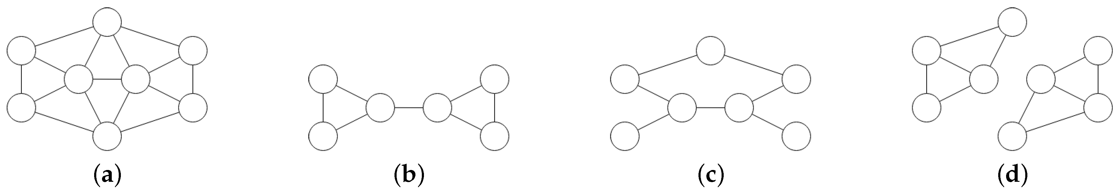
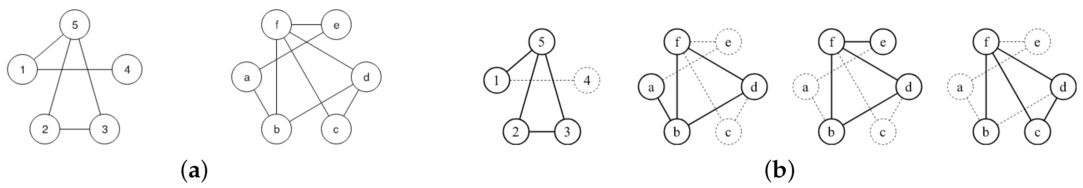
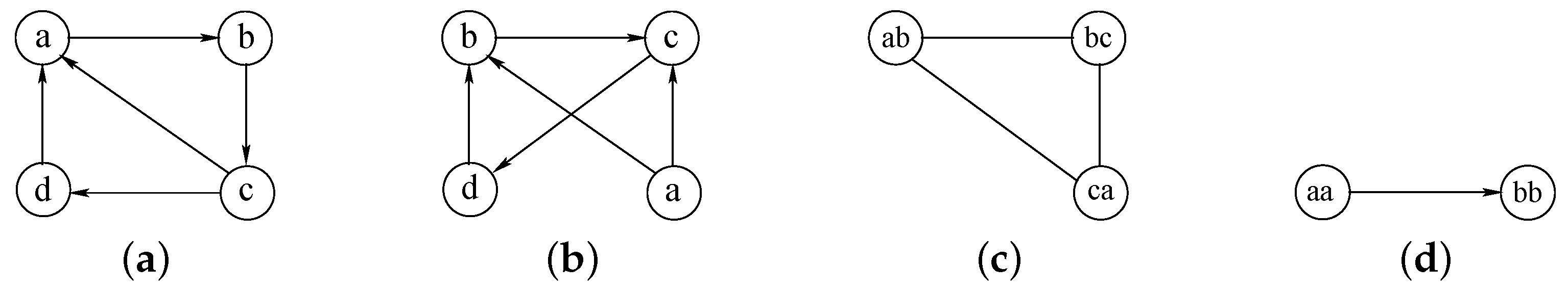
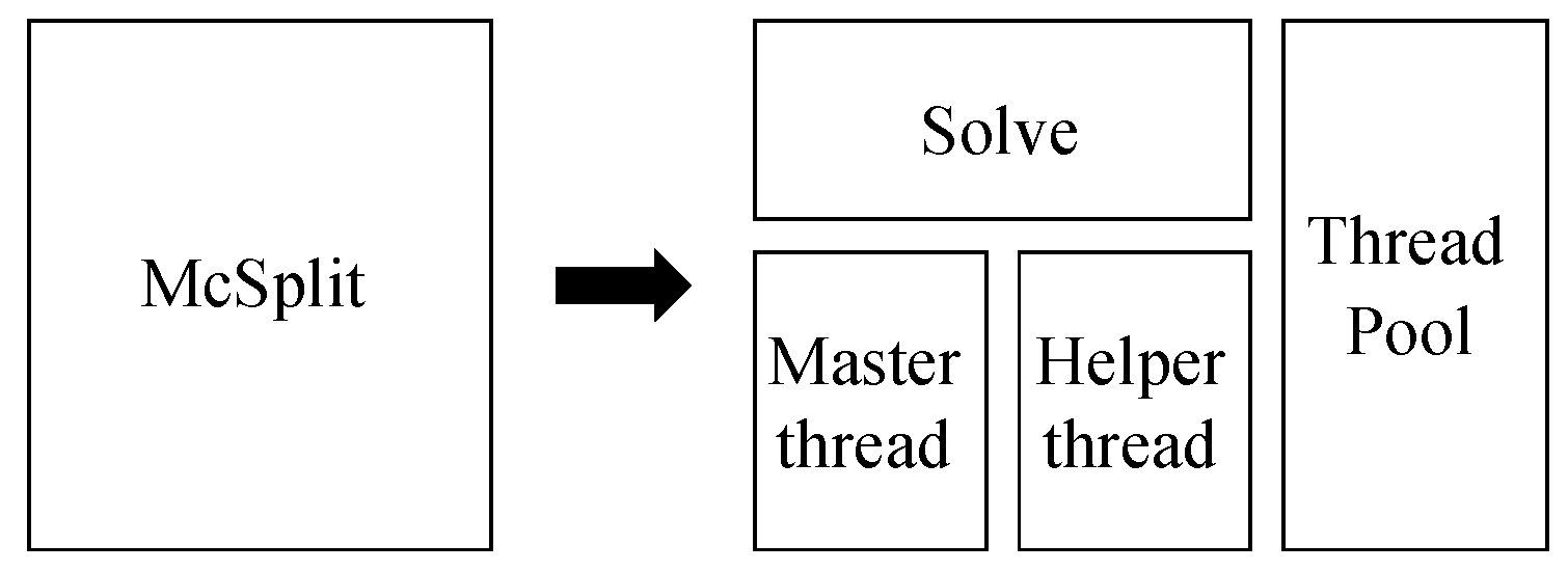
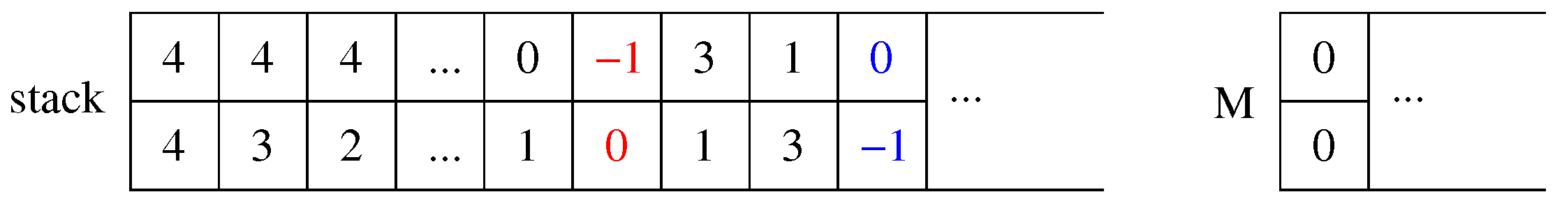
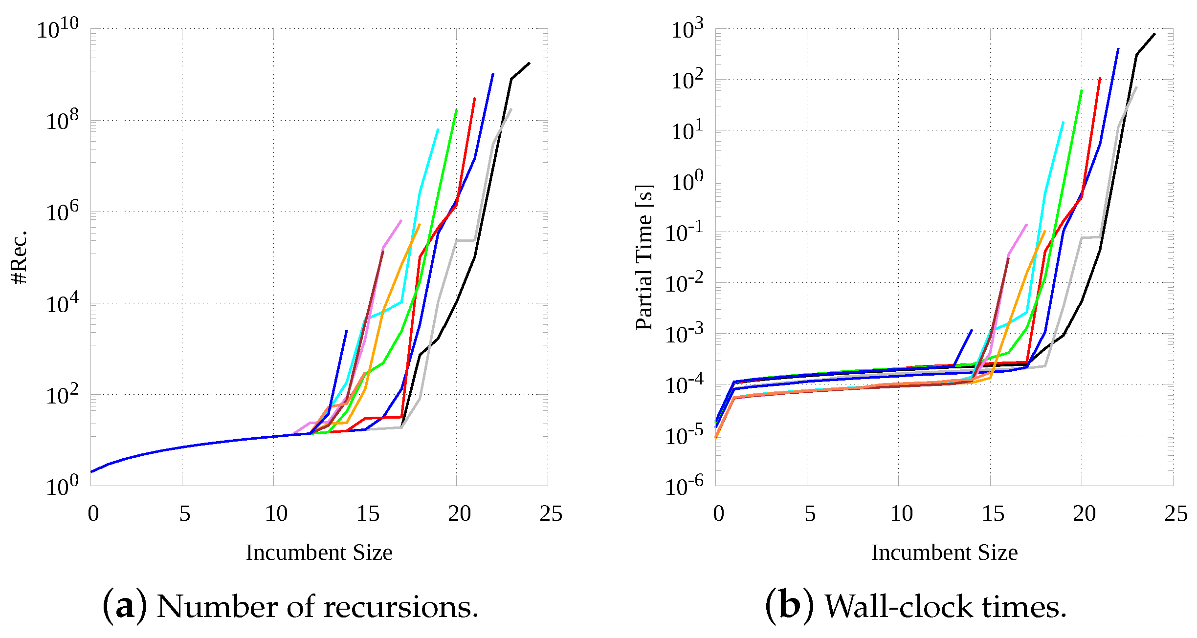
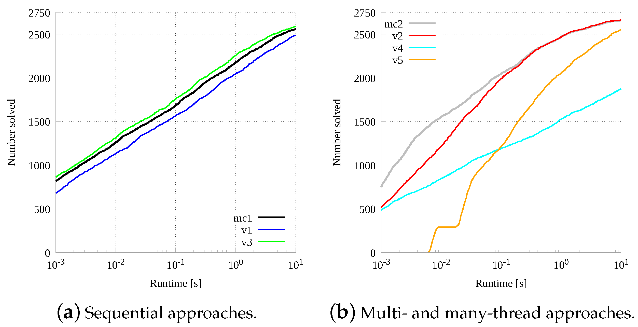
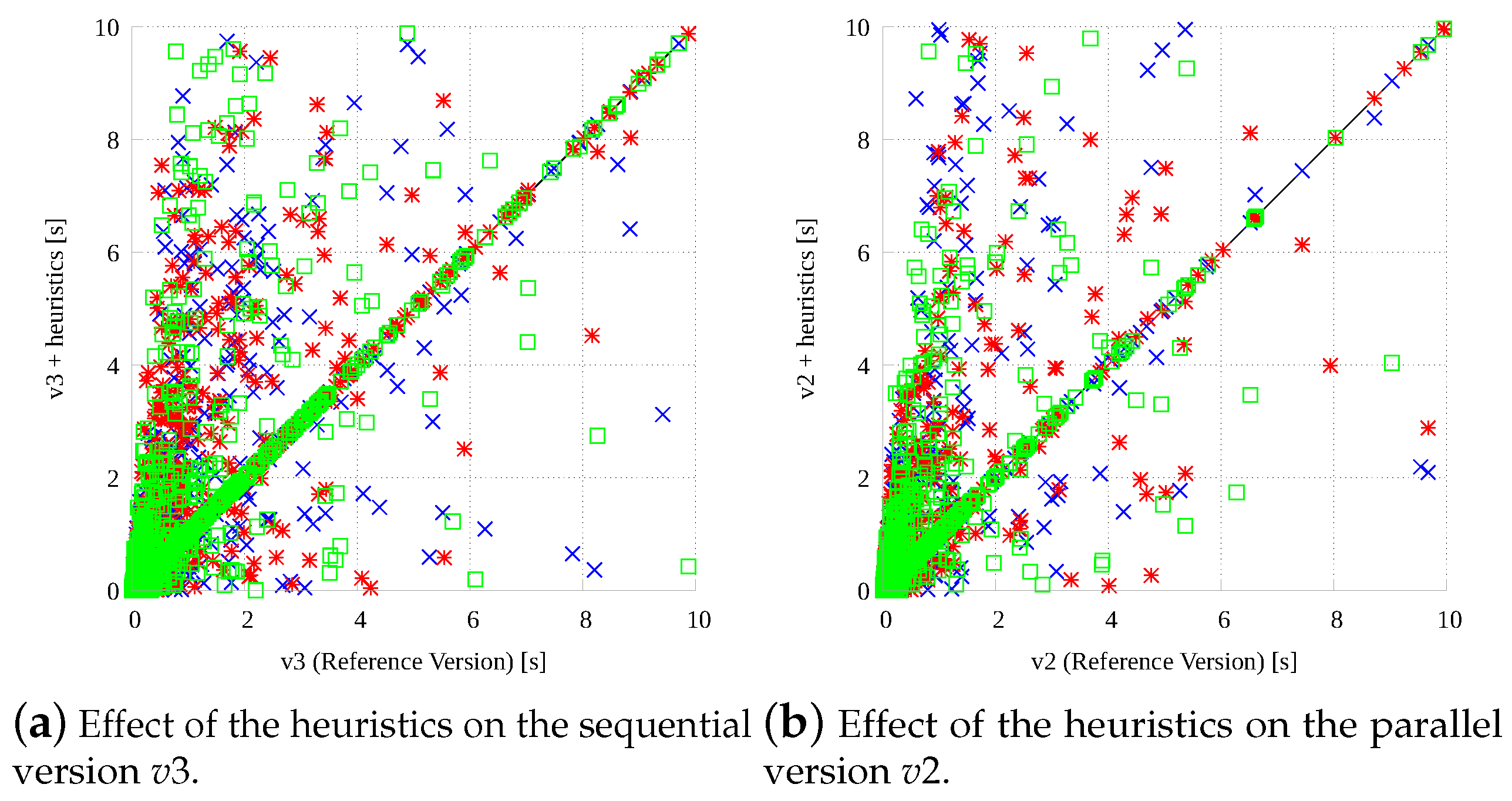
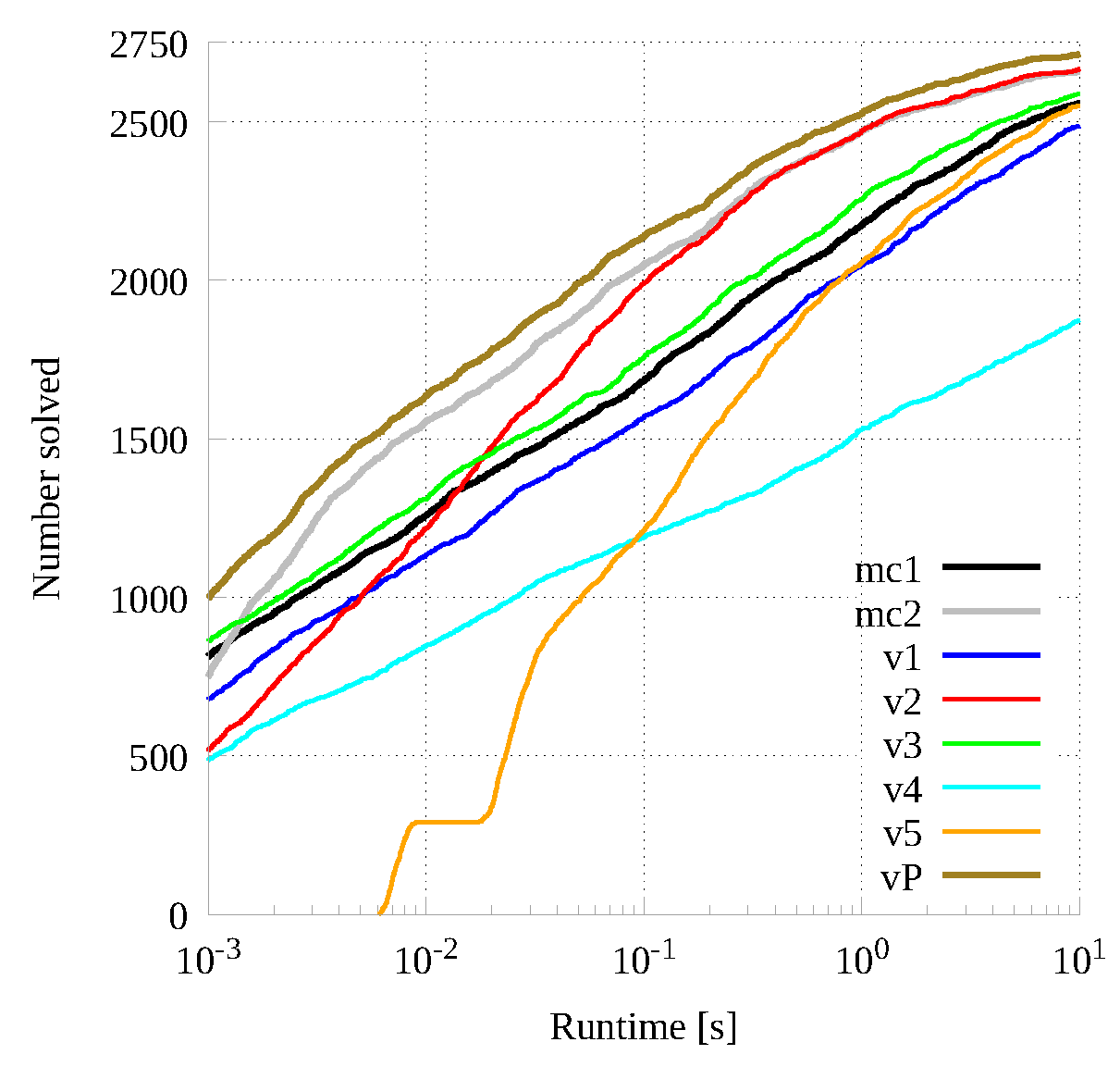
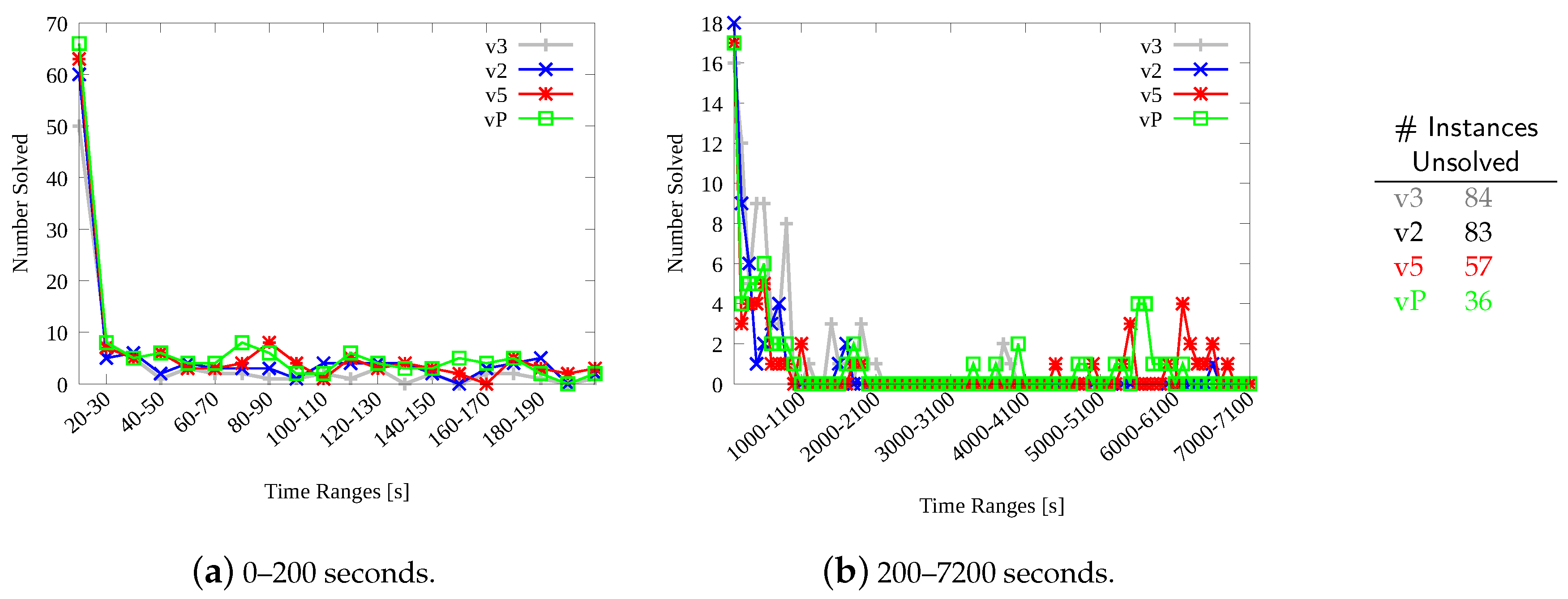
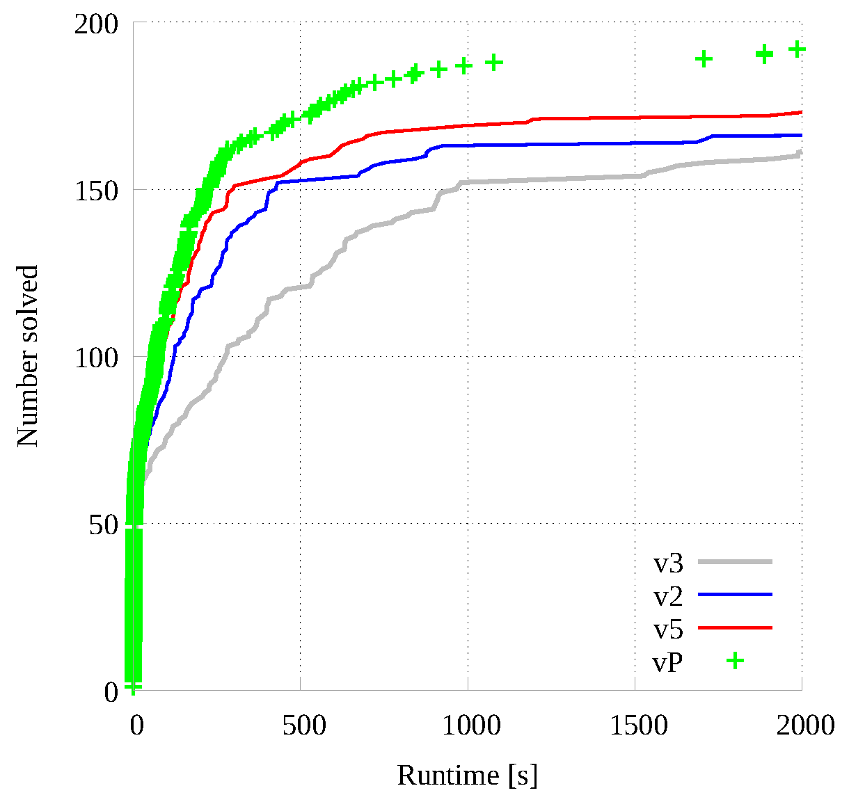
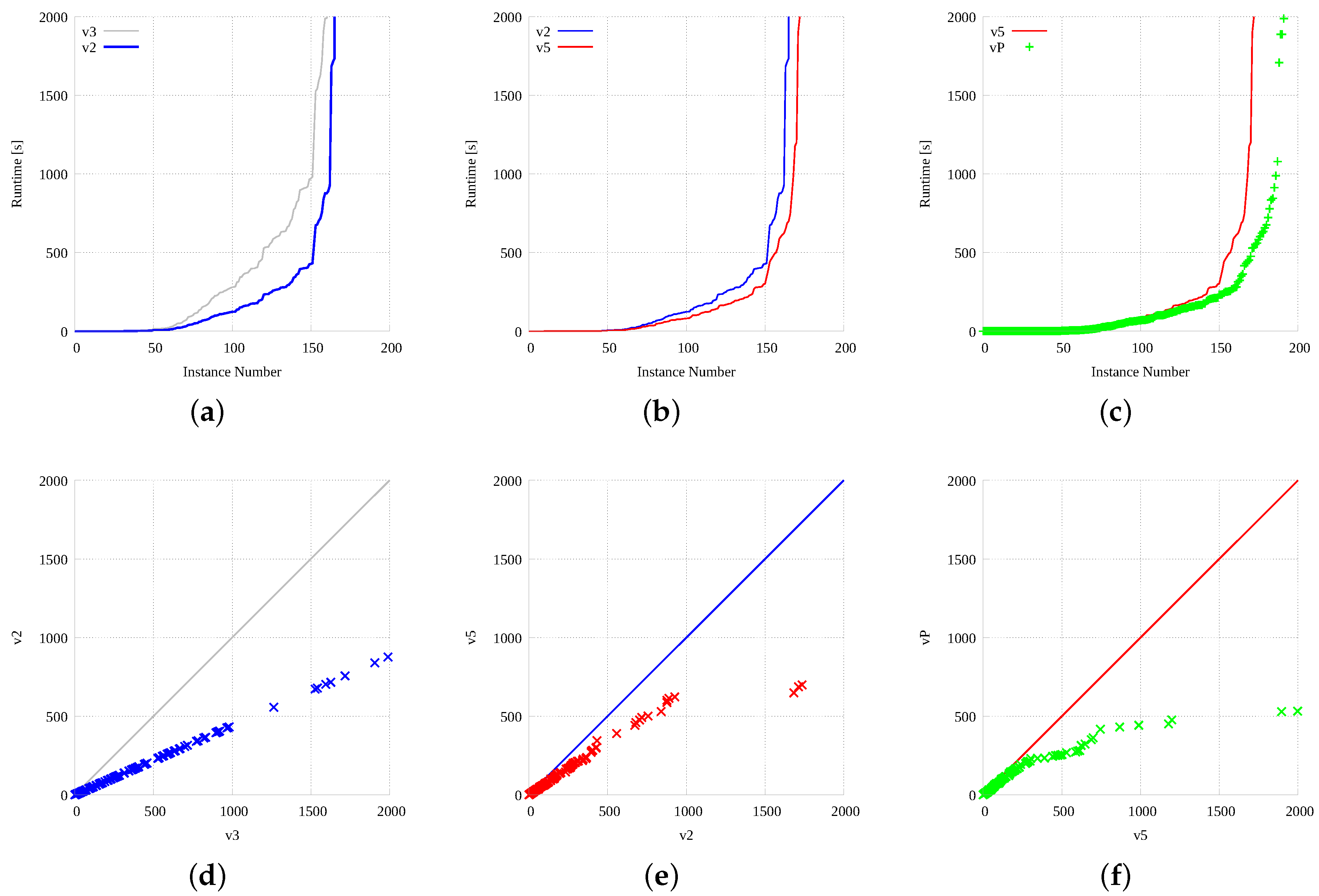
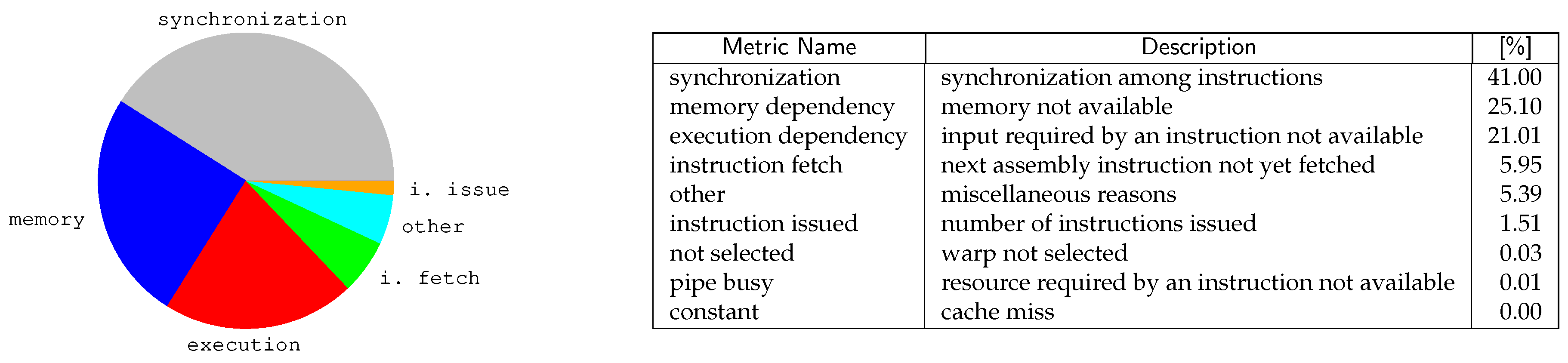
Table 1.
Labels on the non-mapped vertices of G and H with mapping: (a) , (b) and (c) .
| (a) | |||
|---|---|---|---|
| v | Label | v | Label |
| b | 1 | c | 1 |
| c | 1 | a | 1 |
| d | 1 | d | 1 |
| (b) | |||
| v | Label | v | Label |
| c | 11 | a | 11 |
| d | 10 | d | 11 |
| (c) | |||
| v | Label | v | Label |
| d | 101 | d | 110 |
Table 2.
Analysis on the impact of heuristics , , and , on the best sequential () and the best parallel () version.
Table 2.
Analysis on the impact of heuristics , , and , on the best sequential () and the best parallel () version.
| 2586 | 2535 | 2538 | 2530 | solved | 2665 | 2636 | 2633 | 2633 |
| 1321 | 1478 | 1595 | 1499 | total time | 822 | 1100 | 1039 | 1027 |
| 0.4798 | 0.5367 | 0.5789 | 0.5442 | avg. time | 0.2984 | 0.3993 | 0.3772 | 0.3731 |
| 273 | 304 | 340 | 352 | # best | 250 | 345 | 331 | 315 |
Table 3.
Extract from the profiling analysis executed by Nsight. The analysis shows the most divergent instructions in our CUDA main code section.
Table 3.
Extract from the profiling analysis executed by Nsight. The analysis shows the most divergent instructions in our CUDA main code section.
| Code Line | Divergence | Total Executions | |
|---|---|---|---|
| [%] | [#] | ||
| 253 | 9.4 | 17,078 | 180,781 |
| 325 | 40.7 | 26,932 | 66,120 |
| 329 | 22.1 | 6806 | 30,819 |
| 334 | 22.3 | 6884 | 30,819 |
© 2020 by the authors. Licensee MDPI, Basel, Switzerland. This article is an open access article distributed under the terms and conditions of the Creative Commons Attribution (CC BY) license (http://creativecommons.org/licenses/by/4.0/).
Share and Cite
MDPI and ACS Style
Quer, S.; Marcelli, A.; Squillero, G. The Maximum Common Subgraph Problem: A Parallel and Multi-Engine Approach. Computation 2020, 8, 48. https://doi.org/10.3390/computation8020048
AMA Style
Quer S, Marcelli A, Squillero G. The Maximum Common Subgraph Problem: A Parallel and Multi-Engine Approach. Computation. 2020; 8(2):48. https://doi.org/10.3390/computation8020048
Chicago/Turabian StyleQuer, Stefano, Andrea Marcelli, and Giovanni Squillero. 2020. "The Maximum Common Subgraph Problem: A Parallel and Multi-Engine Approach" Computation 8, no. 2: 48. https://doi.org/10.3390/computation8020048
Note that from the first issue of 2016, this journal uses article numbers instead of page numbers. See further details here.