Point-of-Care Using Vis-NIR Spectroscopy for White Blood Cell Count Analysis ^†

Abstract

Total white blood cells count is an important diagnostic parameter in both human and veterinary medicines. State-of-the-art is performed by flow cytometry combined with light scattering or impedance measurements. Spectroscopy point-of-care has the advantages of miniaturization, low sampling, and real-time hemogram analysis. While white blood cells are in low proportions, while red blood cells and bilirubin dominate spectral information, complicating detection in blood. We performed a feasibility study for the direct detection of white blood cells counts in canine blood by visible-near infrared spectroscopy for veterinary applications, benchmarking current chemometrics techniques (similarity, global and local partial least squares, artificial neural networks and least-squares support vector machines) with self-learning artificial intelligence, introducing data augmentation to overcome the hurdle of knowledge representativity. White blood cells count information is present in the recorded spectra, allowing significant discrimination and equivalence between hemogram and spectra principal component scores. Chemometrics methods correlate white blood cells count to spectral features but with lower accuracy. Self-Learning Artificial Intelligence has the highest correlation (0.8478) and a small standard error of 6.92 × 10${}^9$ cells/L, corresponding to a mean absolute percentage error of 25.37%. Such allows the accurate diagnosis of white blood cells in the range of values of the reference interval (5.6 to 17.8 × 10${}^9$ cells/L) and above. This research is an important step toward the existence of a miniaturized spectral point-of-care hemogram analyzer.

1. Introduction

Blood spectra information is characterized by multi-scale interference and matrix effects. These are considered the main limitations toward the existence of spectral point-of-care (POC) technologies, being characterized as violations of the Beer–Lambert law (BLL). Multi-scale interference is the result of overlapping spectral bands of different constituents, their concentration, and molar extinction coefficients, resulting in interference at different intensities observed in the spectra signal [1]. Matrix effects influence the molecular bonds of pure constituents or even lead to reactions that change their original absorbance bands and scattering effects (Mie and Rayleigh) [2,3].

The most common approaches to mitigate spectral interference in analytical chemistry and clinical analysis is to decrease sample complexity by separation and lab-on-a-chip technologies [4] or through reaction specificity biological biochips (e.g., immunological reactions) [5,6,7]. These approaches do not take advantage of the information-rich spectroscopy signal, which provides qualitative and quantitative information about a significant number of constituents in the same measurement [8].

The combination of signal processing, chemometrics, and artificial intelligence in biosensors is improving the accuracy of existing technologies by allowing signal corrections and pattern recognitions that quantify and diagnose clinical conditions, e.g., infection [9] or cancer [10]. Solving multi-scale information and matrix effects in spectroscopy [11,12,13] allows one to explore information-rich features in each sample spectra and to develop the next generation of reagent-less POC technologies.

White Blood Cells and Blood Spectroscopy

A visible near-infrared (Vis-NIR) spectroscopy signal carries both physical (e.g., scattering, reflectance, shadows) and chemical information (e.g., absorbance, fluorescence). The information about a constituent is distributed along the different wavelengths at different scales of intensity. Furthermore, this information is highly auto-correlated due to the superposition and convolution of both optical instrumentation and quantum uncertainty into large continuous spectral bands [14]. Dominant information in blood spectra is attributed to constituents that are highly absorbent in the Vis-NIR region: hemoglobin (Hgb) [15] and bilirubin (Bil) [16]. Red blood cells (RBC) are the dominant cells, and Hgb dominates absorbance/transmittance spectra. Constituents in lower concentrations or with lower absorbance/transmittance appear in the spectra as interferences in the dominant spectral features (e.g., Bil interference with Hgb [15]).

Total white blood cells (WBC) count is one of the most requested hematology parameters because of its broad diagnostic value, including for infection and leukemia. Leukocytosis and leukopenia, which are abnormal values (high/low, respectively) in WBC counts, are frequently associated with neutrophil changes, although other leukocytes and neoplastic cells can also cause fluctuations. Neutrophilia is usually related to inflammation, and neutropenia is usually related to greater peripheral use or reduced bone marrow production [17].

The most common methods for WBC differential are based on electrical impedance, laser light scattering, radiofrequency conductivity, and/or flow cytometry [18]. The basic principles of operation for automated hematology analyzers are based on cell size, directly affecting impedance and scattering angle. This approach has disadvantages for WBC differential, because cell sizes for each leukocyte type are highly dependent on the development stage and differentiation, leading to inaccurate counts in current automated equipment [19]. Despite laser scattering technology providing better accuracy than impedance technology, the latter is widely adopted in veterinary medicine. Impedance counting is an economically advantageous technology, and the best hematology practices recommend blood smear microscope counts on abnormal cases to confirm results [20].

WBC spectroscopy is a valuable diagnostic tool in medicine. Terentyeva (2016) [21] has shown the capacity of ultra-violet visible (UV-Vis) spectroscopy to discriminate leukocytes organelles (cytosol, nuclei, mitochondria, and membranes), as optical centers are able to discriminate between normal and abnormal cells. Changes in absorbance (200–400 nm) and the fluorescence/phosphofluorescence of WBC correspond to significant changes in organelle composition, allowing the diagnosis of chronic lymphocytes leukemia B-cells. Infrared spectroscopy for WBC has also been used in leukemia diagnosis [22,23,24] as well as disease progression monitoring [25,26,27,28]. Inaccessible infection diagnosis using infrared microscope spectroscopy of WBC components enables the determination of an infection source from viral and bacterial agents through support vector machines (SVM) [29].

Figure 1a shows the current state-of-the-art in hemogram quantification using flow cytometry with light scattering or impedance detection and microscopy blood smear count. These are non-portable technologies for the clinical laboratory, and they are very difficult to miniaturize. Oppositely, spectroscopy has no restrictions on the amount of sample as well as no use of reagents, making it ideal for portable POC technology. Figure 1b shows the prototype system, which uses Internet of Things (IoT) electronics and software, being controlled with a smartphone without requiring a dedicated application. A single drop of blood (∼10 $\mathsf{\mu }$L) is placed in a plug-in, re-usable capsule, which is inserted at the transmittance probe tip [30,31]. Capsules are designed with opposing mirrors to maximize internal reflections, and light is captured by a center pinhole fiber optics connected to the spectrometer working within the 300–800 nm range [30].

WBC is in a significantly lower number than RBC (∼1:1000). These are considerably harder to detect in the spectrum, and as a consequence, WBC information is a small percentage of spectral variance when compared to the RBC dominance. For this reason, state-of-the-art chemometrics and artificial intelligence technologies are currently unable to deal with small-scale interference and non-dominant spectral information sample constituents with good accuracy [14]. In special cases, there is a high correlation between RBC and WBC. If a subset is composed of solely these samples, WBC quantification is most likely quantified using the hemoglobin bands, resulting in a statistically valid model, but without causal interpretation. This biased subset can create the illusion of low detection limits, as the visible spectra are very sensitive to hemoglobin. Chemometrics or AI models that rely on data intrinsic correlations and do not hold causal relationships to the constituent should be used with caution, as high bias may occur if an unknown sample is out of the spectral characteristics of this subset [14].

Spectral POC hemogram analysis was developed for measuring RBC, Hgb and HTC in dog and cat blood [31]. The following MAPE metrics were achieved: (i) Dog blood: RBC (6.39%), Hgb (7.14%), hematocrit (HTC) (4.43%); (ii) cat blood: RBC (5.67%), Hgb (4.08%) and HTC (1.69%). RBC, Hgb and HTC are absorbance dominant. These are very well detected by Vis-SWNIR by spectral POC, allowing an accurate diagnosis at both high and low boundaries of the reference interval. MAPE at the higher and lower boundaries of the RI are 4% to 11%, allowing an accurate diagnosis [31]. These results were achieved using a new spectral processing methodology—self-learning artificial intelligence (SLAI), based on the search for covariance modes (CovM). A CovM is a subset of samples that can directly relate the concentration of the constituents to directly relate the concentration of the constituents to spectral interference features, isolating samples that preserve the same type of interference that sustain consistent quantification. CovM also reduce the dimensionality into local feature spaces that describe the particular bands that interfere, allowing both statistical and causal validation and interpretation [14].

The search for CovM is easier to understand considering pure constituents. As these do not hold interference, the covariance between concentration and spectral variance is maximal and holds a direct causal relationship between spectral bands gradients and concentration, as described by the Beer–Lambert law (BLL). Thus, the information contained in compositional changes and spectral bands is the same, only expressed into different basis and units (e.g., signal intensity at each wavelength vs. WBC concentration). This relationship is vectorial and the eigenstructure is unidimensional, being described by the molar extinction coefficient of the constituent, where concentrations are proportional to this vector basis [13,14,31].

In complex samples, e.g., blood, multi-scaled interferences arise from overlapping bands and distortions due to matrix effects (e.g., pH, scattering). Quantitative and qualitative interference information is continuous and spreads along all wavelengths. As biological variance is significantly large, the covariance of large/representative datasets is unstable and presents high dimensionality. This makes it necessary to unscramble the different types of interference that accurately relate the quantitative information of a particular constituent in the context of their interferents by searching for the CovM it belongs to [14]. The CovM is given by a group of samples that provide the same information between spectral interference features and constituent concentration, isolating a particular interference mode present in the dataset.

Each CovM sample has stable covariance between spectra ($\mathbf{X}$) and constituents ($\mathbf{Y}$) information. Such also implies that the information is similar but expressed on a different basis (wavelengths and concentrations). Therefore, the two information blocks exhibit latent structural similarity ($\mathbf{t}\sim \mathbf{u}$), where $\mathbf{t}$ and $\mathbf{u}$ are derived independently from singular value decomposition of $\mathbf{X}$ and $\mathbf{Y}$, where: $\mathbf{X}=\mathbf{T}{\mathbf{P}}^t$ and $\mathbf{Y}=\mathbf{U}{\mathbf{Q}}^t$; being $\mathbf{P}$ and $\mathbf{Q}$ the orthogonal basis of $\mathbf{T}$ and $\mathbf{U}$, respectively. Ideally, at each CovM, interference information is equivalent to the concentration ($\mathbf{t}\sim \mathbf{u}$), being described by a single eigenvector or 1 LV, providing a causal interpretation of spectral interference by cross-referencing the absorbance bands of constituents [1] holding the BLL relationship [13,31].

The objectives of this research are the demonstration of the main challenges faced to directly quantify non-dominant blood constituents, e.g., WBC, and the feasibility of using CovM search for accurate results. In this reasoning, we benchmark current state-of-the-art methods, e.g., similarity (SIM), partial least squares (PLS), local partial least squares (LocPLS), artificial neural networks (ANN) with the input of scores of PCA (PCA-ANN) and PLS (PLS-ANN), and least squares support vector machines (LS-SVM). We further investigate the feasibility of data augmentation as an information enhancement methodology, mitigating class imbalance characteristic of complex biological samples, e.g., canine blood.

2. Methods

2.1. Hemogram Analysis

Dog blood samples, already used in diagnostic clinical procedures, were collected from the jugular vein by qualified personnel using standardized venipuncture procedures at the Centro Hospitalar Veterinário do Porto. Remaining blood from EDTA tubes, previously collected but still fresh, were afterwards used for these assays. Hemogram parameters were determined using a Mindray BC-2800-vet auto-hematology analyzer (Mindray, Shenzhen, China) [32].

2.2. Spectroscopy

Figure 1b shows the Vis-SWNIR POC IoT prototype platform AgIoT2020 [33], using a spectrometer socket adapter (e.g., Hamamatsu C12666MA (Hamamatsu, Hamamatsu, Japan)) or USB based (e.g., Ocean Insight STS-Vis (Ocean Insite, Orlando, FL, USA)) and managing multiple light sources (e.g., LED and laser diodes). The specific version uses a power led (4500 K) at optimized temperature and power modulation. The optical configuration uses transmittance fiber optics with six illumination fibers and a center collection fiber, where a plug-in capsule containing the blood sample is docked. The capsules are built using opposing mirrors (path length of 5 mm) [30]. The average of three spectra was taken from EDTA blood samples and scatter corrected before further analysis [34]. Three replicates of 67 dog blood samples were used in this study out of a total of 201 spectral records.

2.3. Benchmarking

CovM search methodology was benchmarked against the following modeling approaches:

• Similarity: Eucledian distance as a metrics of the spectral and compositional similarity between neighboring samples in the feature space (e.g., [35,36]);
• Partial least squares (PLS): maximizes the covariance between the spectra $\mathbf{X}$ and blood WBC composition $\mathbf{Y}$ by determining the eigenvectors of ${\mathbf{X}}^t\mathbf{Y}$. This method forces the latent structures of spectra and composition (PLS scores—$\mathbf{U}$) to be equal (NIPALS algorithm) [37] for the determination of each correspondent basis ${\mathbf{U}}^t$ and ${\mathbf{Q}}^t$ [38]. It proceeds with deflation and sequential orthogonal eigenvectors of the remaining information in ${\mathbf{X}}^t\mathbf{Y}$ [37,39]. The number of deflations or latent variables are optimized by cross-validation/hold-out samples minimal predicted sum of squares (PRESS) [40]. PLS uses an oblique projection to determine the ${\mathbf{b}}_{pls}$ coefficients in $\mathbf{Y}={\mathbf{Xb}}_{pls}$ [37,39].
• Local PLS (LocPLS): uses KNN clustering to create local sub-groups, where local PLS models are optimized. The KNN clusters are obtained in the PCA scores space. The number of clusters and number of principal components (PC) is optimized by cross-validation/hold-out samples [41];
• Artificial neural networks (ANN): were introduced in spectroscopy as an approach to deal with non-linearity. ANN is a piece-wise linear combination of non-linear activation functions at each node (or neuron) of the network, being parameters optimized by back-propagation. Most ANNs in spectroscopy use PCA or PLS scores as input, being designated PCA-ANN and PLS-ANN [42,43]. The number of LV and ANN architecture (variables and layers) have to be optimized. In this research, we applied the most used template: (i) input layer—coordinates in the LV; (ii) hidden layer—optimized between two and three layers; and (iii) one output node—the estimation of WBC. The tangent and identity functions were used as hidden and output layer activation, respectively. ANN was regressed by back-propagation using the Levenberg–Marquardt algorithm;
• Least-squares support vector machines (LS-SVM): was introduced in spectroscopy to deal with the high non-linearity of feature spaces due to interference. SVM maps similarity between samples using the kernel function, mapping it into a new feature space, where the Gaussian radial basis function (RBF) maps the PLS scores ($\mathbf{U}$). The LS-SVM replaces the e-sensitive loss function by the square loss function to optimize the Karush–Kuhn–Tucker (KKT) linear system obtained by Lagrangian multipliers methodology [44]. At each U comprising an increasing number of LVs, the LS-SVM optimizes the RBF kernel width parameter ($\sigma$) and the regularization parameter of the KKT linear system ($\gamma$) [45]. The number of LV used to compute the kernel matrix is obtained by cross-validation/hold-out sample validation. LS-SVM was implemented using the kernlab library for R [46].

The standard error (SE), mean absolute percentage error (MAPE) and Pearson correlation (R) are presented for each model.

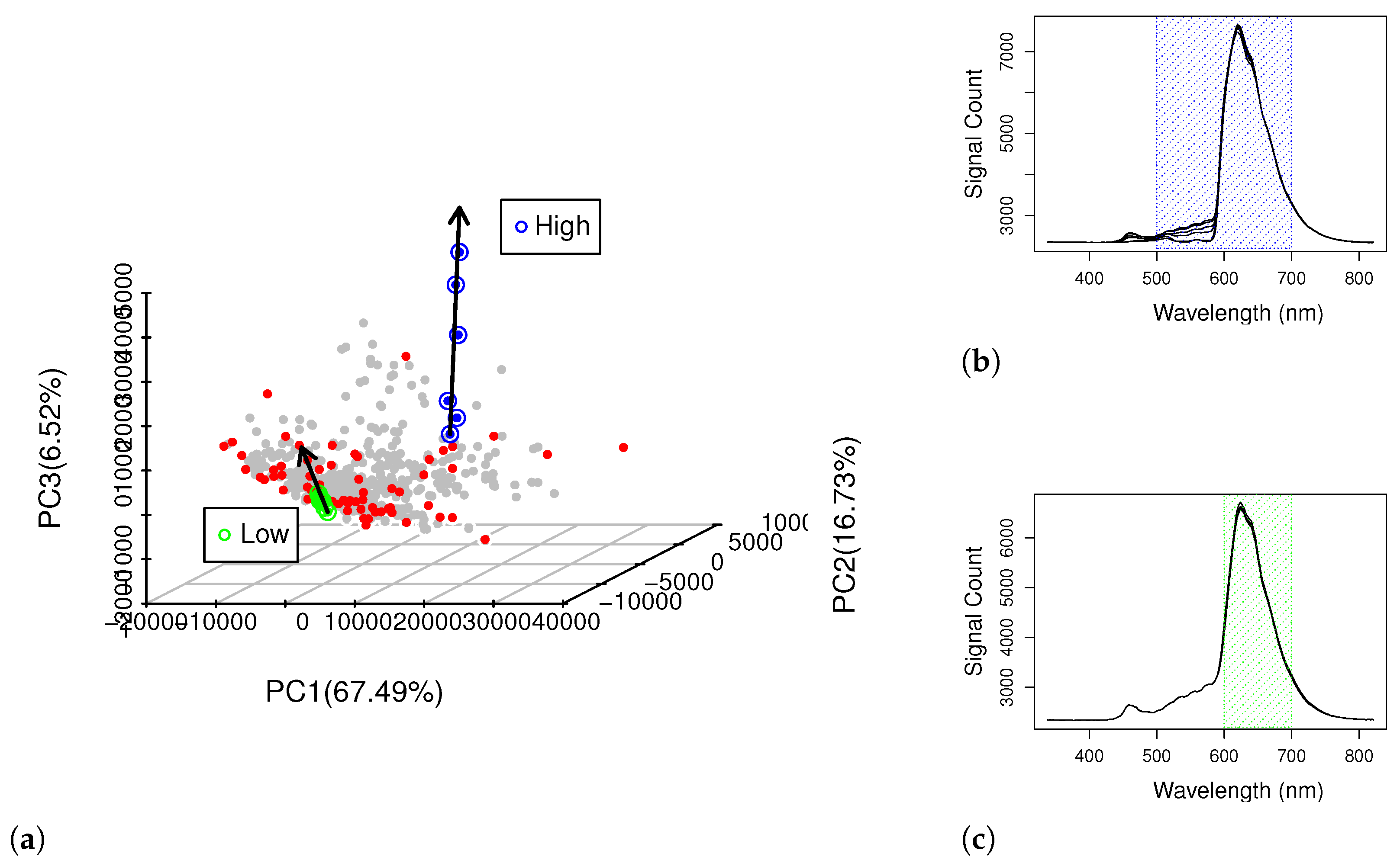
2.4. Covariance Mode Search

The basic principle of SLAI is the search for systematic and stable covariance between composition and spectral features [14]. Stable covariance has a direct relationship to the BLL, and SLAI uses this relationship to unscramble the complex multi-scale interference between blood constituents to quantify RBC, Hgb and HTC. Such is performed in two different steps:

• Feature space optimization: information about a constituent is present in the spectra in different scales and wavelengths. Selecting the correct features and transforms (e.g., singular value decomposition, Fourier or wavelets transforms) is essential to extract the information into a feature space that holds proportionality to the concentration of the constituents; and
• Covariance mode search: searching a group of samples within the feature space that belong to the same interference pattern. Such means that spectral features $\mathbf{X}$ hold the same information as composition $\mathbf{Y}$, with a stable covariance ${\mathbf{X}}^t\mathbf{Y}$.

The SLAI method searches the neighbors of a given sample in all directions to find a group of stable covariance with WBC. This group of samples already provides a quantification, but the method further optimizes the sub-space to find samples that hold the same gradient information between RBC and spectrum features, allowing a very accurate quantification. This sub-space is considered the covariance mode (CovM), where the latent structures of the spectrum features and composition are equivalent, allowing a direct relationship and the interpretation of interference; on the account that covariance is expressed in a single eigenvector, the relation has high accuracy.

2.5. Validation

All models were constructed and validated using a two-step approach: (i) cross-validation to optimize model parameters within the training set; and (ii) prediction for hold-out samples (HO) to estimate the error. Cross-validation (CV) is a hypothesis test to the null hypothesis, that is, the sample being present in the model dataset or not being present, a statistically similar result is expected or the effect is null. By leaving several samples out of model estimation, CV provides the error estimated for each sample in the training set if this sample is unknown, allowing one to decide which are the optimal parameters of each model that best depict the representative features of the dataset and not particularities of each sample (aka overfitting). If the dataset and model are representative, the null effect is expected when using the model to predict hold-out datasets, holding similar error results to the training dataset. CV is used to avoid over-optimization to the dataset (overfitting), and hold-out samples (HO) for null hypothesis testing, determining the generalization of the chosen model. Non-optimal models are more robust to generalization at the cost of accuracy, being an important trade-off when dealing with data scarcity.

Models are chosen for optimal generalization at minimum prediction error of CV (e.g., LV in PLS, ANN architecture). In the case of local methods (Local-PLS and CovM search), the leave-one-out CV and one HO sample were used due to the lower amount of data of the group of samples. Method performance was evaluated by computing the standard deviation (SE), the mean absolute percentage error (MAPE), and the Pearson correlation (R) as a metric of linearity between predicted and measured values. All models were constructed with the median spectra and validated using the leave-one-out cross-validation. CRAN-R was used for all computations (PLSR and NEURALNET packages; LocPLS, Similarity and SLAI using the authors code) [46].

2.6. Spectral Data Augmentation

Data augmentation increases the knowledge base diversity for improving model prediction accuracy [47,48]. It is especially relevant for spectroscopic blood analysis, because the high biological variance is difficult to be fully characterized by proof-of-concept experimental designs, as these are limited to a low number of samples. We refer to the experimental dataset as the real-world knowledge base dataset (RWD).

Herein, we introduce the concept of an ‘in silico’ synthetic spectroscopy dataset (SSD) as an augmentation technique for improving the spectral quantification of WBC. The SSD is computed using the random mixture of spectra and the WBC of two random real-world samples, producing an average spectrum and WBC as synthetic information for the SSD. This procedure is equivalent to mixing two samples physically, because under an ideal mixture assumption spectral information would have direct correspondence to WBC. Mixture samples are non-naturally occurring samples. For example, the blood of an animal never has the properties of the mixture of the blood of two different animals. By mixing ’in silico’ the information of real samples, the knowledge base has new samples that cover spectral gradients, providing the covariance information between spectral features and blood composition which otherwise would not be present in the RWD. A total of 500 SSD samples were obtained by mixing random pairwise RWD samples of spectra (X) and hemogram (Y), where $X_{SSD}=\frac{1}{2}(Xi+Xj)$ and $Y_{SSD}=\frac{1}{2}(Yi+Yj)$, being i and j random blood samples (Figure S1).

SSD is an independent dataset from RWD, where the information about RWD spectral gradients are expected to be preserved. Thus, models optimized using solely the SSD should be resentative of RWD covariance. Furthermore, with the higher spectral variance representativity of the SSD, higher prediction accuracies are expected when compared to using only RWD.

3. Results and Discussion

3.1. WBC Blood Spectroscopy

WBC are in a significantly less number than RBC and lack a chromophore distinct from hemoglobin, which would allow detection sensitivity in the UV-Vis. Instead, WBC information is spread along the 200 to 800 nm as interferences to hemoglobin [21]. This is observable in Figure 2a where dog blood with high WBC has significant absorbance in the 400 to 600 nm—region of interest 1 (ROI 1), whereas, low WBC show higher variance in the range of 600 to 800 nm (ROI 2, Figure 2a). ROI 1 is interferent with Hgb species that have peak absorbance from 500 to 600 nm [15,31] and Bil [16], and interference with WBC information enabling quantification must be investigated. The evaluation of the information structure equivalence between hemograms and spectral data is paramount because WBC is super-imposed and interferent to the other blood constituents.

Figure 2b,c present the three PC of the hemogram and spectra datasets from PCA analysis. PCA obtains orthogonal eigenvectors of a particular dataset by maximizing its variance, being one of the most widely used methods for the characterization of information structure in chemometrics. If one considers $\mathbf{X}$ the spectra (samples x wavelengths) and $\mathbf{Y}$ the hemogram (samples x RGB, Hgb, HTC and WBC) datasets, then the PCA decomposition is as follows: $\mathbf{X}=\mathbf{T}{\mathbf{P}}^t$ and $\mathbf{X}=\mathbf{U}{\mathbf{C}}^t$, where $\mathbf{T}$ and $\mathbf{U}$ are the coordinates in basis ${\mathbf{P}}^t$ and ${\mathbf{C}}^t$, respectively. If $\mathbf{X}$ and $\mathbf{Y}$ share a significant degree of common information, their variance has similar eigenstructure, and therefore, the coordinates $\mathbf{T}$ and $\mathbf{U}$ should be arranged in a qualitative similarity arrangement, despite the different basis being ${\mathbf{P}}^t$ and ${\mathbf{C}}^t$ [14]. The dominant loadings in hemogram data PCA are RBC and WBC, exhibiting a negative correlation (Figure 2b). The ratio WBC to RBC increases, as higher levels of WBC are observed. The scores coordinates allow the direct discrimination of hemograms with high (>$20\times {10}^9$ cells/L) and low (<$8.0\times {10}^9$ cells/L) levels of WBC, and the WBC loading vector provides a satisfactory quantitative interpretation of the WBC in the $\mathbf{U}$ scores space.

The spectral variance scores space ($\mathbf{T}$) is presented in Figure 2c (PC1 (67.49%), PC2 (16.73%) and PC3 (6.52%)). Similar to $\mathbf{U}$, the $\mathbf{T}$ space provides also discrimination between low and high WBC. Despite the high variance due to other blood constituents information present in the spectra, there is a gradient variation of spectral features related to WBC around a vector from low to high WBC (Figure 2c). Furthermore, samples are grouped from high (∼20 × 10${}^9$ cells/L) to extreme (∼70 × 10${}^9$ cells/L) WBC values.

As spectra carry more information than the hemogram, the variance of $\mathbf{T}$ is higher than $\mathbf{U}$, being the hemogram information a partial representation of blood composition. The higher amount of information in $\mathbf{T}$ implies that not all information in the spectra variance space is used to quantify WBC; only the relevant covariance that relates spectral gradient to WBC provides equivalence $\mathbf{T}\sim \mathbf{U}$—the CovM.

WBC and RBC present significant differences in terms of light-scattering characteristics. The scattering coefficient (S) is defined as the ratio $S=2\pi r/\lambda$; where r is the particle radius and $\lambda$ is the wavelength. The RBC radius in dogs is ∼7020 nm, and WBC ∼20,000 nm. As $S\gg$ 1, geometric scattering is dominant in dog blood in UV-Vis spectroscopy. The WBC surface area exposed to light is approximately 2152 $\mathsf{\mu }$m${}^2$, whereas that of RBC is 307 $\mathsf{\mu }$m${}^2$. WBC has eight times more area exposed to light than RBC. Such means the light exposure ratio of WBC to RBC surface areas can range from 0.65% for combinations of low WBC (4 × 10${}^9$ cells/L) and high RBC (5 × 10${}^{12}$ cell/L) to 30% at high WBC levels (70 × 10${}^9$ cell/L) and low RBC levels (2 × 10${}^{12}$ cell/L).

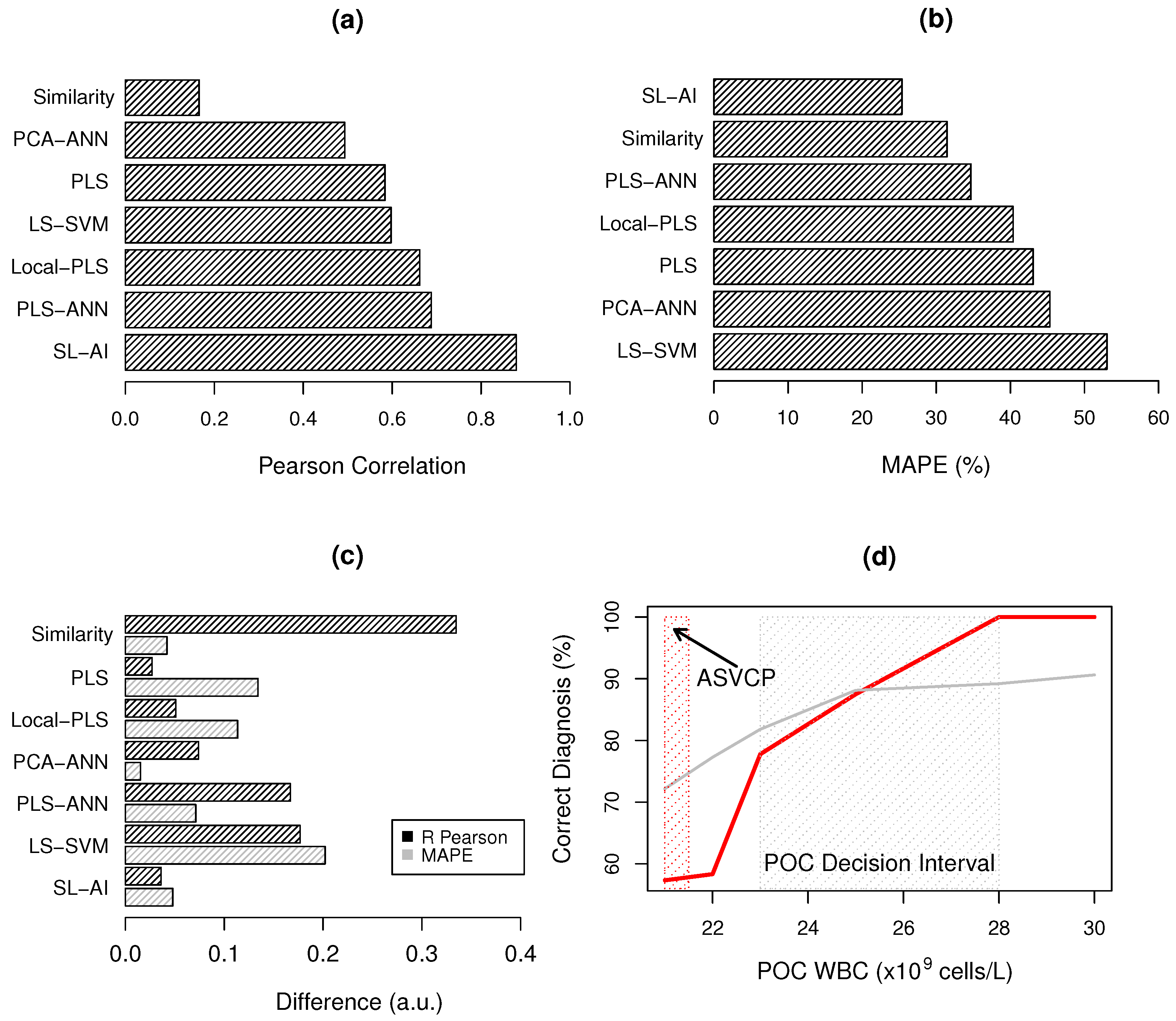
3.2. WBC Quantification

SIM was optimized using three neighboring samples, taking the Euclidean distance in the 3PC scores space, totaling 90.74% of spectral variance (Figure 2c). SIM has a low correlation and high error values (R = 0.4503, MAPE = 37.10%) (

Table 1. WBC quantification metrics using mixture and real datasets.

Method	Parameters	Dataset	R	SE (${10}^9$ Cells/L)	MAPE (%)
SIM	nPC = 3	Mixture	0.5005	8.16	35.66
	n = 3	Real	0.1658	15.66	31.45
PLS	LV = 6	Mixture	0.6109	6.87	29.66
		Real	0.5838	10.92	43.08
LocPLS	LV = 5	Mixture	0.6110	6.52	28.51
		Real	0.6619	10.10	40.37
PCA-ANN	LV = 3	Mixture	0.4197	8.01	46.85
	(8:18:12) ${}^{\left(1\right)}$	Real	0.4934	12.39	45.32
PLS-ANN	LV = 3	Mixture	0.5210	7.60	41.79
	(18:20:15) ${}^{\left(1\right)}$	Real	0.6879	9.02	34.67
LS-SVM		Mixture	0.4207	7.80	32.83
		Real	0.5976	7.50	53.04
SLAI	LV = 1	Mixture	0.8432	4.67	20.57
	nCov = 100	Real	0.8789	6.92	25.37

⁽¹⁾ Network hidden layer architecture; nPC—number of principal components. n—number of neighbors; nCovM—number of CovMs.

, Figure 3a). There is a high discrepancy between real and mixture datasets in terms of Pearson correlation coefficient (R). This low performance is because the Euclidean distance in the $\mathbf{T}$ space does not directly correspond solely to WBC information, and spectral variance (${\mathbf{X}}^t\mathbf{X}$) is not directly related to covariance (${\mathbf{X}}^t\mathbf{Y}$). Results for spectral POC hemogram of RBC, Hgb, and HTC [31] also demonstrated that spectral similarity cannot represent the first principles of the BLL.

PLS has significant correlation (R = 0.6069) but high prediction errors (MAPE = 31.09%) (Table 1, Figure 3b). The Pearson correlation for real (R = 0.6109) and mixture (R = 0.5838) datasets is similar, but PLS has very different error performances between the two datasets (MAPE of 43.08% and 29.66%, respectively) (Table 1). A PLS model was obtained using six LVs. The high number of LVs has implications in the interpretation of the PLS coefficients (${\mathbf{b}}_{pls}$). By adding new dimensions, more interferences are accounted for WBC quantification, resulting in a weighted oblique projection of all existing covariance modes [14,31]. As the eigenstructure of $\mathbf{X}$ is similar to $\mathbf{Y}$, the PLS algorithm is able to converge into an acceptable correlation value. As there are many types of spectral gradients due to interference, PLS is not able to take into account the details of each CovM. PLS is extremely effective when the global covariance (${\mathbf{X}}^t\mathbf{Y}$) is stable, that is, when interference is restricted to a small number of CovM, where the variance of samples is not complex (e.g., high purity chemical product), which is not the case of blood samples. PLS shows that there is a global correlation between spectral information and WBC. The smaller scale of variance in spectroscopy signal due to WBC concerning RBC and Hgb implies that the PLS model needs high dimensionality (6 LVs) to best represent the information. PLS is unable to further increase dimensionality without overfitting, because many CovM do not share the same ROIs used to quantify WBC.

LocPLS has better performance than PLS, with an R = 0.6612 and MAPE = 29.83% (Table 1, Figure 3c). It also has a good correlation agreement between real (R = 0.6619) and mixture datasets (R = 0.6110) but significant differences in terms of MAPE values (40.37% and 28.51%) (Table 1). LocPLS breaks down the complexity of the global covariance (${\mathbf{X}}^t\mathbf{Y}$) into an ensemble of PLS models along the spectral variance space $\mathbf{T}$, considering that a subset of similar samples may hold stable covariance. We also expected a significant reduction in the dimensionality of the PLS models, but results show a modest decrease to five LVs (see Table 1) and no significant gains in correlation (R) or prediction errors (MAPE) compared to PLS. LocPLS does not perform a systematic search for stable covariance, but it uses similarity metrics (Euclidean distance) to group samples. These may or may not belong to the same CovM, resulting in a non-systematic dimension reduction and model performance. LocPLS efficiency is higher in blood constituents that have dominant information in the spectra (e.g., RBC, Hgb, and HTC) [31], not being effective with non-dominant constituents, e.g., WBC.

SIM, PLS and LocPLS cannot model extreme high values of WBC, which have outlier characteristics to the rest of the datasets. Two extreme groups with WBC in the range of 40 to 70 × 10${}^9$ cells/L are outliers to the main model (Figure 3a–c). The high-dimensionality of PLS and LocPLS (6 and 5 LVs, respectively) does not capture the CovM to which these samples should be associated to predict WBC accurately.

ANN (PCA-ANN and PLS-ANN) exhibit low performance when modeling WBC spectral information compared to SIM, PLS, and LocPLS. The Pearson correlation (R) is 0.4214 and 0.5412 for PCA-ANN and PLS-ANN. Prediction errors are high, with an MAPE of 37.33% and 32.63% for PCA-ANN and PLS-ANN (Figure 3d). Both ANN models were optimized with three LVs and architecture of three hidden layers (Table 1). The performance of ANN models is consistent between the real and mixture datasets, showing that the information is similar between datasets, obtaining the same level of performance. PLS-ANN has a better performance than PCA-ANN, because PLS scores are obtained maximizing the covariance, whereas PCA maximizes the variance of the spectral datasets. ANN has high difficulty in finding consistent covariance, especially with low levels of spectral variance of WBC. As ANN is designed using piecewise linear and activation functions, they have better performance mapping non-linear phenomena to which there are clear decision boundaries between classes. PCA-ANN and PLS-ANN showed satisfactory performances only when modeling dominant spectral information, e.g., RGB, Hgb and HTC [31]. ANN approaches struggle to cope with multi-scale interference of non-dominant blood constituents, e.g., WBC.

LS-SVM exhibits poor correlations (R = 0.4372) and high prediction errors (MAPE = 41.35%) (Figure 3f). It also has high discrepancies between the real and mixture datasets, with R values of 0.5976 and 0.4207; and MAPE of 53.04% and 32.83%. LS-SVM has to use a significant number of samples as support vectors, providing more representation of the real than the mixture dataset. Figure 3f shows that LS-SVM has a significant number of outliers at both high and low WBC levels, not modeling extreme WBC values. The Gaussian RBF is used to convert the PLS scores space $\mathbf{U}$ into the SVM kernel matrix. This fails to capture groups of systematic covariance because the RBF can also be considered as a similarity metric.

SLAI presents significant correlations (R = 0.8478) and low prediction errors (MAPE = 20.94) (Figure 3g). Furthermore, it also has results between real and mixture datasets: (i) R: 0.8789 and 0.8432; and (ii) MAPE: 25.37% and 20.57%, respectively. SLAI reduces the dimensionality to 1 LV, being able to determine 100 CovM among the two datasets. The capacity to model extreme values of WBC is significantly improved, where WBC levels between 40 and 70 ×10${}^9$ cells/L are predicted with significantly less error, allowing to correctly diagnose high levels of WBC.

All presented models CV and hold-out samples results have been shown to have statistically similar R, SE and MAPE (p < 0.05).

3.3. Bias-Variance Analysis

POC WBC quantification linearity (Pearson correlation—R) and total error (MAPE) benchmarks are presented in Figure 4a,b. Only SLAI, PLS-ANN, and LocPLS have correlations above 0.60, where SLAI excels with an R = 0.8789 (Figure 3a, Table 1). SLAI also has the lowest total error, with an MAPE of 25.37%, whereas SIM (MAPE = 31.45%), PLS-ANN (MAPE = 34.67%) and LocPLS (MAPE = 40.37%). SLAI has the highest consistency of results metrics (R and MAPE) between the real and mixture datasets. Other consistent methods are PLS and LocPLS, whereas all other methods are not.

Quantitative information about WBC are present in the specific interference gradient of ROIs. As the mixture dataset is obtained by mixing real data, the WBC and spectral gradients are expected to be reasonably preserved, and the information of the mixture dataset represents the real data. Both SLAI, LocPLS, and PLS algorithms maximize covariance, being able to take advantage of the spectral gradients information expansion given by the mixture dataset.

Data augmentation by a random mixture of real data can preserve the spectral information structure, allowing one to complete the necessary information in the knowledge base for complex biological samples, e.g., dog blood. This is particularly relevant for dataset gaps, such as the lack of information on WBC between 40 and 70 ×10${}^9$ cells/L in the real dataset. The mixture of extreme values with lower WBC samples is not free of distortions, affecting model performance. Data augmentation is a trade-off—without filling the information gap, it would be difficult to derive local relationships between extreme WBC values and other samples. The presented data augmentation method is a first proof-of-concept approach that in our opinion should be expanded as a way to complete complex biological datasets, where anomalous samples are rare, and therefore, difficult to be covered by restricted datasets.

Bias analysis was performed by determining the percentage of results that comply with the American Society for Veterinary Clinical Pathology (ASVCP) allowable total error (ATE) quality criteria for WBC: (i) Optimal (Opt): 7.16%; (ii) Desired (Des): 14.29%; and (iii) Acceptable (Accep): 21.45% (see

Table 2. Bias analysis for dog WBC using spectroscopy POC—percentage of results in optimal, desired and acceptable categories.

	Real						Mixture
Method	% Inside RI			% Outside RI			% Inside RI			% Outside RI
	Opt	Des	Accep	Opt	Des	Accep	Opt	Des	Accep	Opt	Des	Accep
SIM	13.30	20.00	30.00	0.00	14.29	14.29	16.72	33.77	40.54	9.75	26.89	34.14
PLS	18.87	30.18	41.51	14.28	21.42	28.57	16.13	32.75	48.13	28.57	40.36	55.10
LocPLS	24.53	41.51	47.17	14.25	28.57	42.85	16.62	30.52	48.63	19.38	36.73	52.34
ANNPCA	14.00	24.00	36.00	0.00	5.88	11.76	15.67	28.85	45.03	24.24	34.34	44.44
ANNPLS	10.15	27.27	41.82	8.33	16.60	33.30	17.04	31.82	45.86	32.35	39.22	40.25
LS-SVM	4.72	14.24	23.81	25.00	25.00	25.00	19.19	33.83	44.94	20.00	30.00	36.60
SLAI	24.53	41.50	58.49	21.42	28.57	42.87	27.36	50.99	66.92	29.59	52.04	72.45

Best bias benchmarks are in bold.

). These criteria are based on veterinary doctor’s expectations in analytical limits for hemogram and other clinical analysis, where: (i) optimal is the best ATE limit for diagnosis, from where there is no clinical advantage in improving the method detection limits; (ii) desired—the limit value of ATE where the clinical decision is still comfortable; and (iii) acceptable—the limit from which the ATE is still valuable for clinical decisions, complementing other sources of clinical information.

State-of-the-art methods—SIM, PLS, PCA-ANN, PLS-ANN, and LS-SVM—present very low levels of acceptable results inside and outside the RI. These methods also show significant inconsistencies between real and mixture datasets (Table 2). Only PLS was able to obtain the best results for the mixture dataset inside (48.13%) and outside (55.10%) RI. LocPLS attained the highest percentage of acceptable results from state-of-the-art methods, with 47.17% and 48.68% (real and mixture) inside the RI; and 42.85% and 52.34% (real and mixture) outside the RI. These results are yet outside the ATE criteria of ASVCP [20].

SLAI has the highest values of acceptable errors ATE for real and mixture datasets (Table 2). In the (i) real dataset, it attains a percentage of 58.49% and 42.87%; and (ii) in the mixture dataset, 66.92%, and 72.45% acceptable results are obtained inside and outside the RI, respectively. Within the desired category, 52.04% of results are outside the RI from the mixture dataset.

SLAI does not yet satisfy the ATE of 21.45%. Only 58.49% of results can pass this criterion (Table 2). The limits imposed for WBC ATE are considered optimistic for the existing technology capabilities, being difficult to achieve even by the ground truth method—microscopy manual counts. It has been widely recognized that both WBC and their differentiated cell counts have high imprecision [20,49,50], and consequently, a wider decision interval should be considered [51]. Figure 4d presents how the number of correct high WBC diagnoses evolves with the WBC predicted by the spectroscopy POC. At the ASCVP ATE limit, the POC is unable to provide enough diagnosis confidence. However, if this boundary is slightly increased to 23 × 10${}^9$ cells/L, the accuracy of the diagnosis rapidly increases to 80% toward 100% of accurate diagnosis at 28 × 10${}^9$ cells/L. As the SLAI is trained with the established technology for hemogram, the present POC results are within today’s state-of-the-art technology capabilites.

3.4. CovM Interpretation

Spectra ROIs allow the interpretation of information used in each CovM WBC model. In addition to statistical validation, these allow the causal relationship by associating ROIs to absorbance and scattering characteristics of the group of samples belonging to a CovM. Figure 5 presents two CovMs at high and low WBC levels. Figure 5a shows the spectra PCA scores space ($\mathbf{T}$) with all datasets, where the low level of WBC CovM samples are in green, and the high-level are in blue. The presented arrows represent the covariance eigenvector (1 LV), correlating WBC to the spectral features. Both high and low WBC CovM eigenvectors point toward increasing values of PC2 and PC3, which is in agreement with the presented PCA scores and loading analysis presented in Figure 2b,c. The directions of each eigenvector are significantly different and represent the ROIs used to quantify WBC. The high WBC CovM sample spectra are presented in Figure 5b, showing that WBC quantification at these levels uses information from 500 to 700 nm. At high levels of WBC (35 to 70 × 10${}^9$ cells/L), very significant absorbance occurs in ROI 1 (400–600 nm) being less pronounced in ROI 2 (600–700 nm). In the low-level WBC CovM, WBC quantification is performed using only ROI 2.

RBC and Hgb absorbance dominates spectral information at low levels of WBC. As WBC spectral information is interferent with RBC and HgB, it is highly difficult to quantify WBC with ROI 1, because the signal variance contribution from WBC is very low. Therefore, at these levels, small-scale WBC information must be found in other ROIs. For this to happen, a group of samples with similar levels of RBC, Hgb, and HTC must be found to determine a small-scale variance in the spectra that corresponds to WBC variance, isolating the information in ROI 2 (Figure 5c). ROI 2 has much less absorbance and interference from RBC and Hgb, and therefore, WBC scattering and absorbance information is being used to quantify at low levels.

At high WBC levels, WBC information has more influence in spectral variance in ROI 1 and 2. The different levels of WBC begin to dominate the spectra in this ROI. More pronounced absorbance is observable at ROI 2 than in low levels of WBC (Figure 5b,c). The robustness of the CovM eigenvector is demonstrated at high-level WBC (Figure 5a): (i) an unknown sample that is under the alignment of the eigenvector can have its WBC value predicted using the information of the other CovM samples; and (ii) the predictability of any sample at a CovM can be assessed by the distance to the eigenvector, that is, any sample that is not in the alignment cannot be predicted accurately [14].

The quantification of low levels of WBC is limited by its small-scale variance in the spectroscopy signal. WBC detection limits are possible to be decreased by: (i) increasing the dataset knowledgbase, to find groups of stable values of RBC, Hgb and HTC, isolating WBC variance; and (ii) reference methods with higher accuracy—proving high statistical robustness to the spectra—WBC relationship.

Current state-of-the-art hemogram instruments or manual counting still cannot decrease the detection limits. It may only be feasible to decrease the spectral POC detection limits when the accuracy of reference methods improves.

4. Conclusions

UV-Vis spectroscopy is a viable POC technology for WBC dog blood hemogram analysis, providing real-time results with a single drop of blood. WBC spectral information is highly interferent with other blood constituents and, therefore, difficult to be unscrambled by the current state-of-the-art chemometrics and machine learning methods. CovMs have the highest result consistency between real and mixture datasets, further proving the relevance of using data augmentation with extreme WBC in restricted data, as a way to complete and expand the knowledgebase information. We also showed the challenges of lowering the POC WBC detection limits. At low WBC levels, more restricted ROIs with smaller scales of spectral variance are expected, implying that RBC/Hgb levels are necessary to isolate WBC spectral information to obtain accurate results.

References

1. Pasquini, C. Near infrared spectroscopy: A mature analytical technique with new perspectives—A review. Anal. Chim. Acta 2018, 1026, 8–36. [Google Scholar] [CrossRef] [PubMed]
2. Olinger, J.M.; Griffiths, P.R. Quantitative effects of an absorbing matrix on near-infrared diffuse reflectance spectra. Anal. Chem. 1988, 60, 2427–2435. [Google Scholar] [CrossRef]
3. Sparén, A.; Hartman, M.; Fransson, M.; Johansson, J.; Svensson, O. Matrix effects in quantitative assessment of pharmaceutical tablets using transmission Raman and Near-Infrared (NIR) Spectroscopy. Appl. Spectrosc. 2015, 69, 580–589. [Google Scholar] [CrossRef] [PubMed]
4. Nishat, S.; Jafry, A.T.; Martinez, A.W.; Awan, F.R. Paper-based microfluidics: Simplified fabrication and assay methods. Sens. Actuators B Chem. 2021, 336, 129681. [Google Scholar] [CrossRef]
5. Zhou, T.; Lu, D.; She, Q.; Chen, C.; Chen, J.; Huang, Z.; Feng, S.; You, R.; Lu, Y. Hypersensitive detection of IL-6 on SERS substrate calibrated by dual model. Sens. Actuators B Chem. 2021, 336, 129597. [Google Scholar] [CrossRef]
6. Jiang, K.; Wu, J.; Qiu, Y.; Go, Y.Y.; Ban, K.; Park, H.J.; Lee, J.H. Plasmonic colorimetric PCR for rapid molecular diagnostic assays. Sens. Actuators B Chem. 2021, 337, 129762. [Google Scholar] [CrossRef]
7. Lewińska, I.; Speichert, M.; Granica, M.; Tymecki, Ł. Colorimetric point-of-care paper-based sensors for urinary creatinine with smartphone readout. Sens. Actuators B Chem. 2021, 340, 129915. [Google Scholar] [CrossRef]
8. Burns, D.; Ciurczak, E. Handbook of Near Infrared Analysis, 2nd ed.; Marcel Dekker, Inc.: New York, NY, USA, 2001. [Google Scholar]
9. Barroso, T.G.; Martins, R.C.; Fernandes, E.; Cardoso, S.; Rivas, J.; Freitas, P.P. Detection of BCG bacteria using a magnetoresistive biosensor: A step towards a fully electronic platform for tuberculosis point-of-care detection. Biosens. Bioelectron. 2018, 100, 259–265. [Google Scholar] [CrossRef] [Green Version]
10. Lin, K.; Cheng, D.L.P.; Huang, Z. Optical diagnosis of laryngeal cancer using high wavenumber Raman spectroscopy. Biosens. Bioelectron. 2012, 35, 213–217. [Google Scholar] [CrossRef]
11. Monteiro-Silva, F.; Jorge, P.A.S.; Martins, R.C. Optical Sensing of Nitrogen, Phosphorus and Potassium: A Spectrophotometrical Approach toward Smart Nutrient Deployment. Chemosensors 2019, 7, 51. [Google Scholar] [CrossRef]
12. Barroso, T.; Ribeiro, L.; Gregório, H.; Santos, F.; Martins, R.C. Point-of-care Vis-SWNIR spectroscopy towards reagent-less hemogram analysis. Sens. Actuators B Chem. 2021, 343, 130138. [Google Scholar] [CrossRef]
13. Martins, R.C.; Barroso, T.; Jorge, P.; Cunha, M.; Santos, F. Unscrambling spectral interference and matrix effects in Vitis vinifera Vis-NIR spectroscopy: Towards analytical grade ‘in vivo’ sugars and acids quantification. Comput. Electron. Agric. 2022, 194, 106710. [Google Scholar] [CrossRef]
14. Martins, R.C. Big Data Self-Learning Artificial Intelligence Methodology for the Accurate Quantification and Classification of Spectral Information under Complex Variability and Multi-Scale Interference. WO/2018/060967, 5 April 2018. [Google Scholar]
15. Philo, J.; Adams, M.; Schuster, T.M. Association-dependent absorption spectra of oxyhemoglobin A and its subunits. J. Biol. Chem. 1981, 256, 7917–7924. [Google Scholar] [CrossRef]
16. Tan, H.; Liao, S.; Pan, T.; Zhang, J.; Chen, J. Rapid and simultaneous analysis of direct and indirect bilirubin indicators in serum through reagent-free visible-near-infrared spectroscopy combined with chemometrics. Spectrochim. Acta A Mol. Biomol. Spectrosc. 2020, 233, 118215. [Google Scholar] [CrossRef] [PubMed]
17. Burton, A.G.; Jandrey, K.E. Leukocytosis and Leukopenia. In Textbook of Small Animal Emergency Medicine; John Wiley & Sons, Ltd.: Hoboken, NJ, USA, 2018; Chapter 64; pp. 405–412. [Google Scholar] [CrossRef]
18. Chabot-Richards, D.S.; George, T.I. White Blood Cell Counts: Reference Methodology. Clin. Lab. Med. 2015, 35, 11–24. [Google Scholar] [CrossRef]
19. Rishniw, M.; Pion, P.D. Evaluation of performance of veterinary in-clinic hematology analyzers. Vet. Clin. Pathol. 2016, 45, 604–614. [Google Scholar] [CrossRef]
20. Nabity, M.B.; Harr, K.E.; Camus, M.S.; Flatland, B.; Vap, L. ASVCP guidelines: Allowable total error hematology. Vet. Clin. Pathol. 2018, 47, 9–21. [Google Scholar] [CrossRef] [Green Version]
21. Terent’yeva, Y.G.; Yashchuk, V.M.; Zaika, L.A.; Snitserova, O.M.; Losytsky, M.Y. The manifestation of optical centers in UV–Vis absorption and luminescence spectra of white blood human cells. Methods Appl. Fluoresc. 2016, 4, 044010. [Google Scholar] [CrossRef]
22. Ramesh, J.; Kapelushnik, J.; Mordehai, J.; Moser, A.; Huleihel, M.; Erukhimovitch, V.; Levi, C.; Mordechai, S. Novel methodology for the follow-up of acute lymphoblastic leukemia using FTIR microspectroscopy. J. Biochem. Biophys. Methods 2002, 51, 251–261. [Google Scholar] [CrossRef]
23. Ramesh, J.; Huleihel, M.; Mordehai, J.; Moser, A.; Erukhimovich, V.; Levi, C.; Kapelushnik, J.; Mordechai, S. Preliminary results of evaluation of progress in chemotherapy for childhood leukemia patients employing Fourier-transform infrared microspectroscopy and cluster analysis. J. Lab. Clin. Med. 2003, 141, 385–394. [Google Scholar] [CrossRef]
24. Liu, W.; Howarth, M.; Greytak, A.B.; Zheng, Y.; Nocera, D.G.; Ting, A.Y.; Bawendi, M.G. Compact biocompatible quantum dots functionalized for cellular imaging. J. Am. Chem. Soc. 2007, 130, 1274–1284. [Google Scholar] [CrossRef] [PubMed] [Green Version]
25. Sahu, R.K.; Zelig, U.; Huleihel, M.; Brosh, N.; Talyshinsky, M.; Ben-Harosh, M.; Mordechai, S.; Kapelushnik, J. Continuous monitoring of WBC (biochemistry) in an adult leukemia patient using advanced FTIR-spectroscopy. Leuk. Res. 2006, 30, 687–693. [Google Scholar] [CrossRef] [PubMed]
26. Zelig, U.; Mordechai, S.; Shubinsky, G.; Sahu, R.K.; Huleihel, M.; Leibovitz, E.; Nathan, I.; Kapelushnik, J. Pre-screening and follow-up of childhood acute leukemia using biochemical infrared analysis of peripheral blood mononuclear cells. Biochim. Biophys. Acta Gen. Subj. 2011, 1810, 827–835. [Google Scholar] [CrossRef] [PubMed]
27. Chaber, R.; Kowal, A.; Jakubczyk, P.; Arthur, C.; Łach, K.; Wojnarowska-Nowak, R.; Kusz, K.; Zawlik, I.; Paszek, S.; Cebulski, J. A Preliminary Study of FTIR Spectroscopy as a Potential Non-Invasive Screening Tool for Pediatric Precursor B Lymphoblastic Leukemia. Molecules 2021, 26, 1174. [Google Scholar] [CrossRef]
28. Kochan, K.; Bedolla, D.E.; Perez-Guaita, D.; Adegoke, J.A.; Veettil, T.C.P.; Martin, M.; Roy, S.; Pebotuwa, S.; Heraud, P.; Wood, B.R. Infrared Spectroscopy of Blood. Appl. Spectrosc. 2021, 75, 611–646. [Google Scholar] [CrossRef]
29. Agbaria, A.H.; Beck, G.; Lapidot, I.; Rich, D.H.; Kapelushnik, J.; Mordechai, S.; Salman, A.; Huleihel, M. Diagnosis of inaccessible infections using infrared microscopy of white blood cells and machine learning algorithms. Analyst 2020, 145, 6955–6967. [Google Scholar] [CrossRef]
30. Martins, R.C.; Sousa, N.; Osorio, R. Optical System for Parameter Characteization of an Element of Body Fluid or Tissue. US10209178B2, 19 February 2019. [Google Scholar]
31. Barroso, T.G.; Ribeiro, L.; Gregório, H.; Santos, F.; Martins, R.C. Visible Near-Infrared Platelets Count: Towards Thrombocytosis Point-of-Care Diagnosis. Chem. Proc. 2021, 5, 78. [Google Scholar] [CrossRef]
32. Brown, M.; Wittwer, C. Flow Cytometry: Principles and Clinical Applications in Hematology. Clin. Chem. 2000, 46, 1221–1229. [Google Scholar] [CrossRef] [Green Version]
33. INESCTEC. AgIoT—Modular Solution and Open Source IoT Solution for Agrofood Domain; INESCTEC: Porto, Portugal, 2020. [Google Scholar]
34. Martens, H.; Stark, E. Extended multiplicative signal correction and spectral interference subtraction: New preprocessing methods for near infrared spectroscopy. J. Pharm. Biomed. Anal. 1991, 9, 625–635. [Google Scholar] [CrossRef]
35. Ramirez-Lopez, L.; Behrens, T.; Schmidt, K.; Stevens, A.; Demattê, J.; Scholten, T. The spectrum-based learner: A new local approach for modelling soil vis-nir spectra of complex datasets. Geoderma 2013, 195–196, 268–279. [Google Scholar] [CrossRef]
36. Fachada, N.; Figueiredo, M.A.; Lopes, V.V.; Martins, R.C.; Rosa, A.C. Spectrometric differentiation of yeast strains using minimum volume increase and minimum direction change clustering criteria. Pattern Recognit. Lett. 2014, 45, 55–61. [Google Scholar] [CrossRef] [Green Version]
37. Ergon, R. Re-interpretation of NIPALS results solves PLSR inconsistency problem. J. Chemo. 2009, 23, 72–75. [Google Scholar] [CrossRef] [Green Version]
38. Geladi, P.; Kowalsky, B. Partial least squares regression: A tutorial. Anal. Chim. Acta 1988, 185, 1–17. [Google Scholar] [CrossRef]
39. Phatak, A.; Jong, S. The geometry of partial least squares. J. Chemom. 1997, 11, 311–338. [Google Scholar] [CrossRef]
40. Krstajic, D.; Buturovic, L.J.; Leahy, D.E.; Thomas, S. Cross-validation pitfalls when selecting and assessing regression and classification models. J. Chemom. 2014, 6, 10. [Google Scholar] [CrossRef] [Green Version]
41. Shen, G.; Lesnoff, M.; Baeten, V.; Dardenne, P.; Davrieux, F.; Ceballos, H.; Belalcazar, J.; Dufour, D.; Yang, Z.; Han, L.; et al. Local partial least squares based on global PLS scores. J. Chemom. 2019, 33, e3117. [Google Scholar] [CrossRef]
42. Janik, L.; Cozzolino, D.; Dambergs, R.; Cynkar, W.; Gishen, M. The prediction of total anthocyanin concentration in red-grape homogenates using visible-near-infrared spectroscopy and artificial neural networks. Anal. Chim. Acta 2013, 594, 107–118. [Google Scholar] [CrossRef]
43. Fernandes, A.; Franco, C.; Mendes-Ferreira, A.; Mendes-Faia, A.; Costa, P.; Melo-Pinto, P. Brix, pH and anthocyanin content determination in whole Port wine grape berries by hyperspectral imaging and neural networks. Comput. Electron. Agric. 2015, 115, 88–96. [Google Scholar] [CrossRef]
44. Suykens, J.; De Brabanter, J.; Lukas, L.; Vandewalle, J. Weighted least squares support vector machines: Robustness and sparse approximation. Neurocomputing 2002, 48, 85–105. [Google Scholar] [CrossRef]
45. Chauchard, F.; Cogdill, R.; Roussel, S.; Roger, J.; Bellon-Maurel, V. Application of LS-SVM to non-linear phenomena in NIR spectroscopy: Development of a robust and portable sensor for acidity prediction in grapes. Chemom. Intell. Lab. Syst. 2004, 71, 141–150. [Google Scholar] [CrossRef] [Green Version]
46. R Core Team. R: A Language and Environment for Statistical Computing; R Foundation for Statistical Computing: Vienna, Austria, 2022; Available online: http://www.r-project.org/ (accessed on 20 August 2022).
47. Nalepa, J.; Marcinkiewicz, M.; Kawulok, M. Data Augmentation for Brain-Tumor Segmentation: A Review. Front. Comput. Neurosci. 2019, 13, 83. [Google Scholar] [CrossRef] [Green Version]
48. Shorten, C.; Khoshgoftaar, T. A survey on Image Data Augmentation for Deep Learning. J. Big Data 2019, 6, 60. [Google Scholar] [CrossRef]
49. Jensen, A.L.; Kjelgaard-Hansen, M. Method comparison in the clinical laboratory. Vet. Clin. Pathol. 2006, 35, 276–286. [Google Scholar] [CrossRef] [PubMed]
50. Cook, A.M.; Moritz, A.; Freeman, K.P.; Bauer, N. Objective evaluation of analyzer performance based on a retrospective meta-analysis of instrument validation studies: Point-of-care hematology analyzers. Vet. Clin. Pathol. 2017, 46, 248–261. [Google Scholar] [CrossRef] [PubMed]
51. Cook, A.M.; Moritz, A.; Freeman, K.P.; Bauer, N. Quality requirements for veterinary hematology analyzers in small animals—A survey about veterinary experts’ requirements and objective evaluation of analyzer performance based on a meta-analysis of method validation studies: Bench top hematology analyzer. Vet. Clin. Pathol. 2016, 45, 466–476. [Google Scholar] [CrossRef]
Figure 1. Total white blood cell counts: (a) current laboratory methods—automated cell counting using electric impedance or laser scattering, and manual blood smear count at the microscope by trained hematologist; and (b) point-of-care approach—single blood drop spectroscopy counts using artificial intelligence (adopted from [12]).
Chemosensors 10 00460 g001
Figure 2. WBC spectral information: (a) dog blood spectra ( low WBC, high WBC and mixture spectra); (b) PCA scores of hemogram counts; and (c) PCA scores of blood spectra, where: mixture of hemogram/spectra samples, blood samples, low WBC and high WBC; hemogram PCA loading.
Chemosensors 10 00460 g002
Figure 3. WBC prediction for: (a) SIM; (b) PLS; (c) LocPLS; (d) PCA-ANN; (e) PLS-ANN; (f) LS-SVM; and (g) SLAI; where () represent the mixture of samples and () blood samples, respectively. Blue shaded rectangle represents the WBC reference interval for dogs (5.6–17.8 × 10 9 cells/L).
Chemosensors 10 00460 g003
Figure 4. WBC quantification benchmarks: (a) Pearson correlation coefficient; (b) MAPE and (c) absolute difference in R and MAPE between mixture and real samples predictions; and (d) percentage of correct diagnosis as function of WBC POC prediction: mixture spectra and real samples.
Chemosensors 10 00460 g004
Figure 5. WBC CovM demonstration: (a) high and low WBC CovMs in PCA scores space— mixture samples, real samples; CovM samples with low WBC, CovM samples with high WBC, and → the CovM vector; (b) High WBC CovM spectra and wavelength variance correlated to WBC (blue rectangle); (c) Low WBC CovM spectra and wavelength variance correlated to WBC (green rectangle).
Chemosensors 10 00460 g005