
Incorporating Robustness to Imaging Physics into Radiomic Feature Selection for Breast Cancer Risk Estimation

 , ,
, ,
Abstract
:Simple Summary
Abstract
1. Introduction
2. Materials and Methods
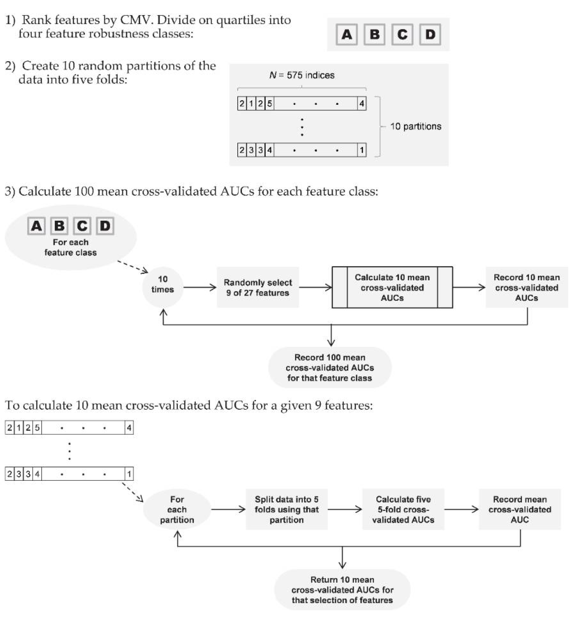
2.1. Roadmap
2.2. Robust Feature Identification
2.2.1. Study Population
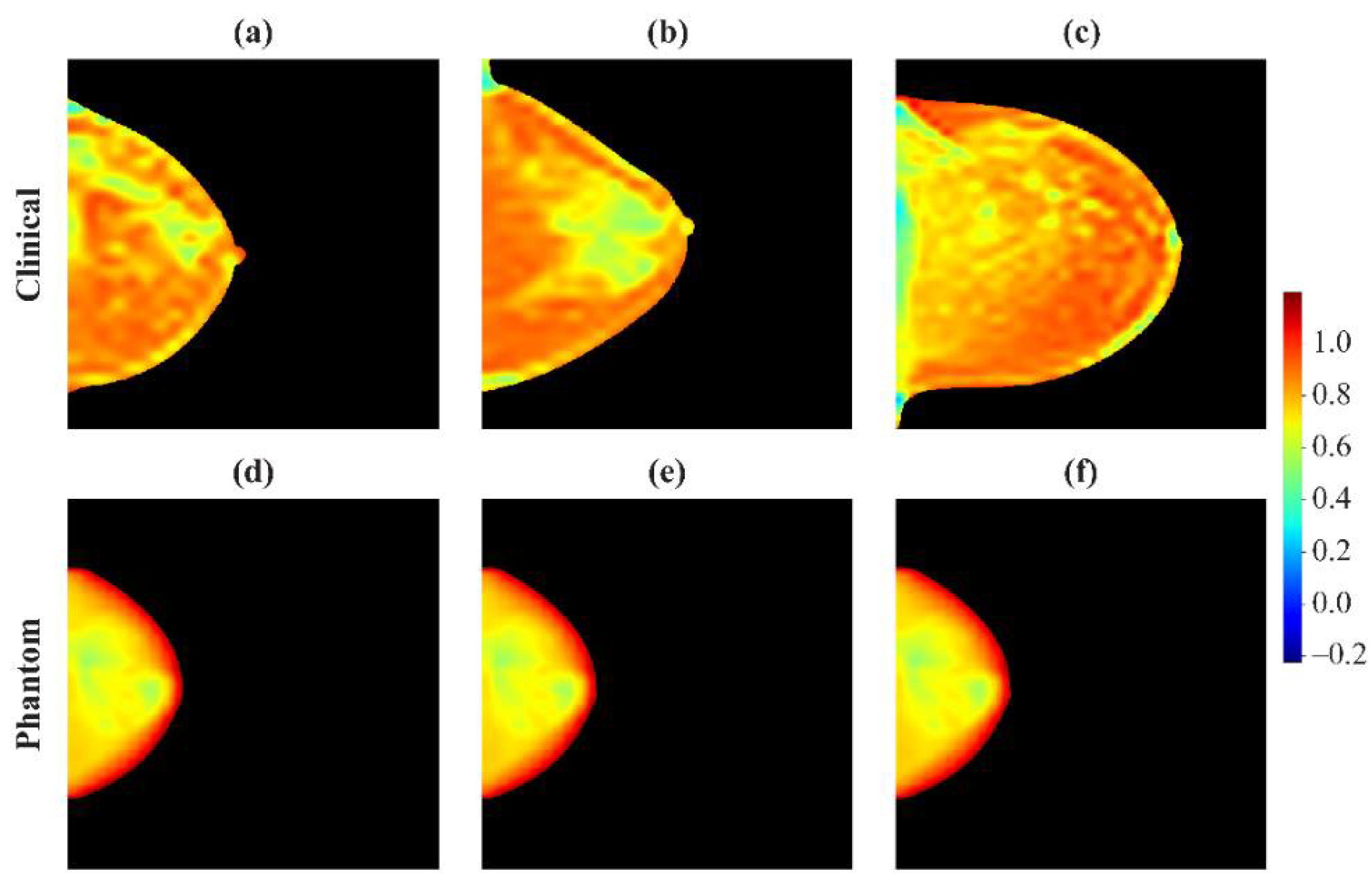
2.2.2. Phantom Data Acquisitions
2.2.3. Feature Extraction
2.2.4. Imaging Acquisition Variation
2.2.5. Intra-Woman Variation
2.2.6. Composite Measure of Variation
2.3. Case-Control Analysis
2.3.1. Study Population
2.3.2. Dimensionality Reduction
2.3.3. Case-Control Classification
3. Results
3.1. Roadmap
3.2. Robust Feature Identification
3.2.1. Study Population
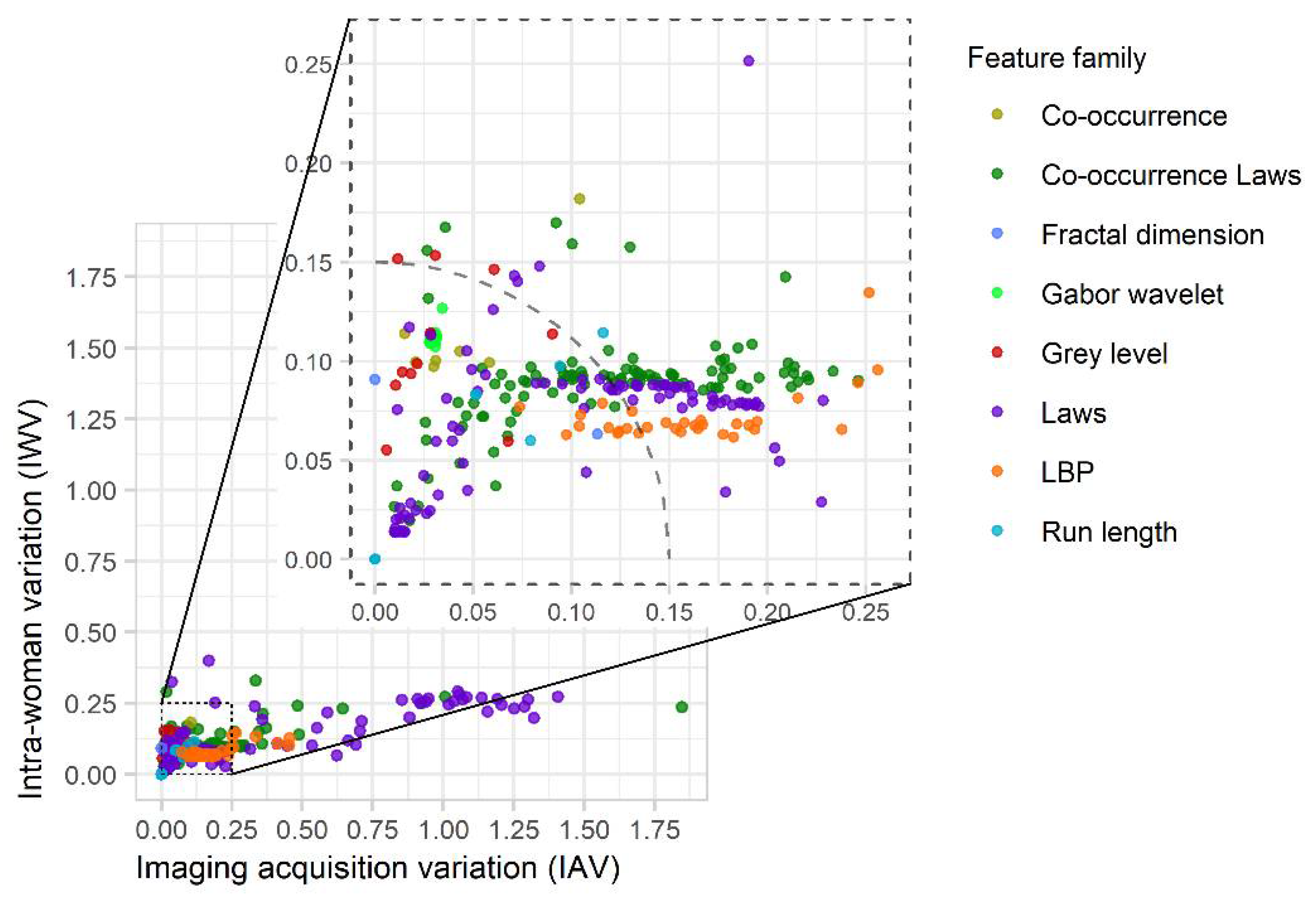
3.2.2. Robustness Calculations
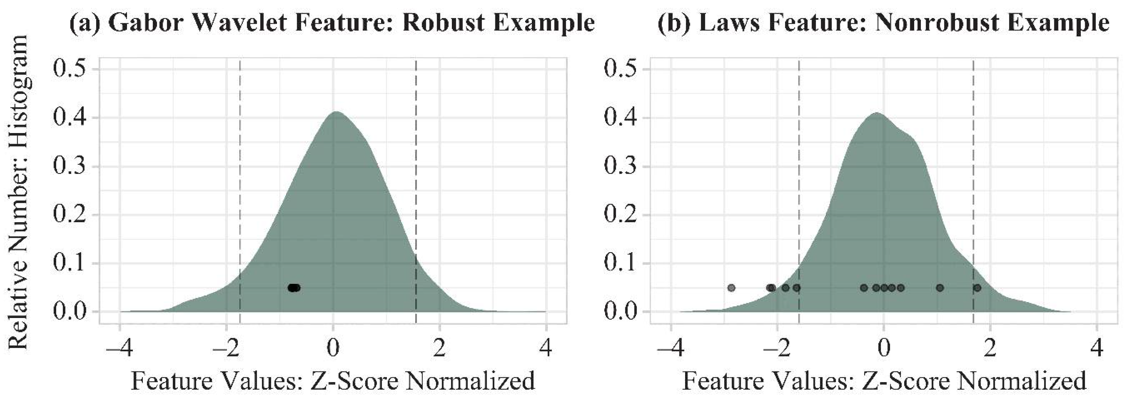
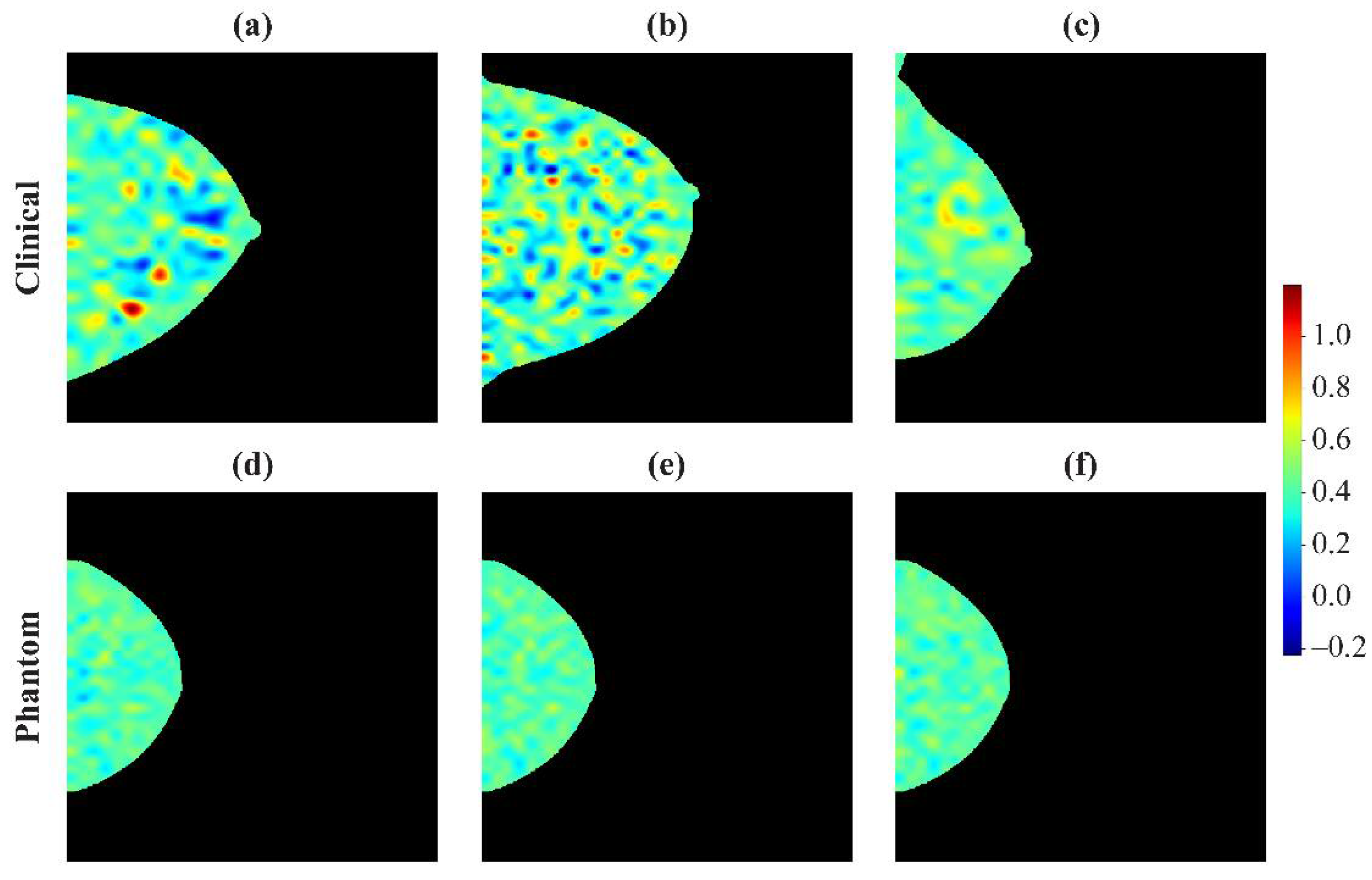
3.2.3. Examples of Robust and Non-Robust Features
3.3. Case-Control Evaluation
3.3.1. Dimensionality Reduction
3.3.2. Performance Evaluation
4. Discussion
5. Conclusions
Supplementary Materials
Author Contributions
Funding
Institutional Review Board Statement
Informed Consent Statement
Data Availability Statement
Conflicts of Interest
References
- Boyd, N.F.; Rommens, J.M.; Vogt, K.; Lee, V.; Hopper, J.L.; Yaffe, M.J.; Paterson, A. Mammographic breast density as an intermediate phenotype for breast cancer. Lancet Oncol. 2005, 6, 798–808. [Google Scholar] [CrossRef]
- Boyd, N.F.; Guo, H.; Martin, L.J.; Sun, L.; Stone, J.; Fishell, E.; Jong, R.A.; Hislop, G.; Chiarelli, A.; Minkin, S.; et al. Mammographic Density and the Risk and Detection of Breast Cancer. N. Engl. J. Med. 2007, 356, 227–236. [Google Scholar] [CrossRef] [PubMed] [Green Version]
- Wanders, J.O.P.; Holland, K.; Karssemeijer, N.; Peeters, P.H.M.; Veldhuis, W.B.; Mann, R.M.; van Gils, C.H. The effect of volumetric breast density on the risk of screen-detected and interval breast cancers: A cohort study. Breast Cancer Res. 2017, 19, 67. [Google Scholar] [CrossRef] [PubMed] [Green Version]
- Zheng, Y.; Keller, B.M.; Ray, S.; Wang, Y.; Conant, E.F.; Gee, J.C.; Kontos, D. Parenchymal texture analysis in digital mammography: A fully automated pipeline for breast cancer risk assessment. Med. Phys. 2015, 42, 4149–4160. [Google Scholar] [CrossRef] [PubMed] [Green Version]
- Gastounioti, A.; Conant, E.F.; Kontos, D. Beyond breast density: A review on the advancing role of parenchymal texture analysis in breast cancer risk assessment. Breast Cancer Res. 2016, 18, 1–12. [Google Scholar] [CrossRef] [Green Version]
- Malkov, S.; Shepherd, J.A.; Scott, C.G.; Tamimi, R.M.; Ma, L.; Bertrand, K.A.; Couch, F.; Jensen, M.R.; Mahmoudzadeh, A.P.; Fan, B.; et al. Mammographic texture and risk of breast cancer by tumor type and estrogen receptor status. Breast Cancer Res. 2016, 18, 122, Erratum in 2017, 19, 1. [Google Scholar] [CrossRef] [Green Version]
- Balagurunathan, Y.; Kumar, V.; Gu, Y.; Kim, J.; Wang, H.; Liu, Y.; Goldgof, D.B.; Hall, L.O.; Korn, R.; Zhao, B.; et al. Test–Retest Reproducibility Analysis of Lung CT Image Features. J. Digit. Imaging 2014, 27, 805–823. [Google Scholar] [CrossRef] [Green Version]
- Zhang, Y.; Oikonomou, A.; Wong, A.; Haider, M.A.; Khalvati, F. Radiomics-based Prognosis Analysis for Non-Small Cell Lung Cancer. Sci. Rep. 2017, 7, srep46349. [Google Scholar] [CrossRef]
- Parmar, C.; Grossmann, P.; Bussink, J.; Lambin, P.; Aerts, H.J.W.L. Machine Learning methods for Quantitative Radiomic Biomarkers. Sci. Rep. 2015, 5, 13087. [Google Scholar] [CrossRef]
- Rizzo, S.; Botta, F.; Raimondi, S.; Origgi, D.; Buscarino, V.; Colarieti, A.; Tomao, F.; Aletti, G.; Zanagnolo, V.; Del Grande, M.; et al. Radiomics of high-grade serous ovarian cancer: Association between quantitative CT features, residual tumour and disease progression within 12 months. Eur. Radiol. 2018, 28, 4849–4859. [Google Scholar] [CrossRef] [PubMed]
- Huynh, E.; Coroller, T.P.; Narayan, V.; Agrawal, V.; Romano, J.; Franco, I.; Parmar, C.; Hou, Y.; Mak, R.H.; Aerts, H.J.W.L. Associations of Radiomic Data Extracted from Static and Respiratory-Gated CT Scans with Disease Recurrence in Lung Cancer Patients Treated with SBRT. PLoS ONE 2017, 12, e0169172. [Google Scholar] [CrossRef] [Green Version]
- Wilkinson, L.; Friendly, M. The History of the Cluster Heat Map. Am. Stat. 2009, 63, 179–184. [Google Scholar] [CrossRef] [Green Version]
- Rizzo, S.; Botta, F.; Raimondi, S.; Origgi, D.; Fanciullo, C.; Morganti, A.G.; Bellomi, M. Radiomics: The facts and the challenges of image analysis. Eur. Radiol. Exp. 2018, 2, 1–8. [Google Scholar] [CrossRef]
- Robinson, K.; Li, H.; Lan, L.; Schacht, D.; Giger, M. Radiomics robustness assessment and classification evaluation: A two-stage method demonstrated on multivendor FFDM. Med. Phys. 2019, 46, 2145–2156. [Google Scholar] [CrossRef]
- Mendel, K.R.; Li, H.; Lan, L.; Cahill, C.M.; Rael, V.; Abe, H.; Giger, M.L. Quantitative texture analysis: Robustness of radiomics across two digital mammography manufacturers’ systems. J. Med. Imaging 2017, 5, 011002. [Google Scholar] [CrossRef]
- Yaffe, M.J.; Johns, P.C.; Nishikawa, R.M.; Mawdsley, G.E.; Caldwell, C.B. Anthropomorphic radiologic phantoms. Radiology 1986, 158, 550–552. [Google Scholar] [CrossRef]
- Keller, B.M.; Oustimov, A.; Wang, Y.; Chen, J.; Acciavatti, R.J.; Zheng, Y.; Ray, S.; Gee, J.C.; Maidment, A.D.A.; Kontos, D. Parenchymal texture analysis in digital mammography: Robust texture feature identification and equivalence across devices. J. Med. Imaging 2015, 2, 24501. [Google Scholar] [CrossRef] [PubMed] [Green Version]
- Conant, E.F.; Keller, B.M.; Pantalone, L.; Gastounioti, A.; McDonald, E.S.; Kontos, D. Agreement between Breast Percentage Density Estimations from Standard-Dose versus Synthetic Digital Mammograms: Results from a Large Screening Cohort Using Automated Measures. Radiology 2017, 283, 673–680. [Google Scholar] [CrossRef] [Green Version]
- Keller, B.M.; Nathan, D.L.; Wang, Y.; Zheng, Y.; Gee, J.C.; Conant, E.F.; Kontos, D. Estimation of breast percent density in raw and processed full field digital mammography images via adaptive fuzzy c-means clustering and support vector machine segmentation. Med. Phys. 2012, 39, 4903–4917. [Google Scholar] [CrossRef] [PubMed] [Green Version]
- Haralick, R.M.; Shanmugam, K.; Dinstein, I. Textural Features for Image Classification. IEEE Trans. Syst. Man. Cybern. 1973, 3, 610–621. [Google Scholar] [CrossRef] [Green Version]
- Galloway, M.M. Texture analysis using gray level run lengths. Comput. Graph. Image Process. 1975, 4, 172–179. [Google Scholar] [CrossRef]
- Chu, A.; Sehgal, C.; Greenleaf, J. Use of gray value distribution of run lengths for texture analysis. Pattern Recognit. Lett. 1990, 11, 415–419. [Google Scholar] [CrossRef]
- Ojala, T.; Pietikainen, M.; Maenpaa, T. Multiresolution gray-scale and rotation invariant texture classification with local binary patterns. IEEE Trans. Pattern Anal. Mach. Intell. 2002, 24, 971–987. [Google Scholar] [CrossRef]
- Manduca, A.; Carston, M.J.; Heine, J.J.; Scott, C.; Pankratz, V.S.; Brandt, K.R.; Sellers, T.A.; Vachon, C.M.; Cerhan, J.R. Texture Features from Mammographic Images and Risk of Breast Cancer. Cancer Epidemiol. Biomarkers Prev. 2009, 18, 837–845. [Google Scholar] [CrossRef] [Green Version]
- Gastounioti, A.; Hsieh, M.-K.; Cohen, E.; Pantalone, L.; Conant, E.F.; Kontos, D. Incorporating Breast Anatomy in Computational Phenotyping of Mammographic Parenchymal Patterns for Breast Cancer Risk Estimation. Sci. Rep. 2018, 8, 1–10. [Google Scholar] [CrossRef] [Green Version]
- Gandrud, C. Reproducible Research with R and R Studio; CRC Press: Boca Raton, FL, USA, 2013. [Google Scholar]
- Acciavatti, R.J.; Gastounioti, A.; Hu, Y.; Maidment, A.D.; Kontos, D.; Chen, J.; Hsieh, M.-K. Validation of the textural realism of a 3D anthropomorphic phantom for digital breast tomosynthesis. In Proceedings of the 14th International Workshop on Breast Imaging (IWBI 2018), Atlanta, GA, USA, 8–11 July 2018; Volume 10718, p. 107180R. [Google Scholar] [CrossRef]
- Andrearczyk, V.; Depeursinge, A.; Müller, H. Neural network training for cross-protocol radiomic feature standardization in computed tomography. J. Med. Imaging 2019, 6, 024008. [Google Scholar] [CrossRef]
- Sechopoulos, I. A review of breast tomosynthesis. Part I. The image acquisition process. Med. Phys. 2013, 40, 014301. [Google Scholar] [CrossRef] [PubMed] [Green Version]
- Sechopoulos, I. A review of breast tomosynthesis. Part II. Image reconstruction, processing and analysis, and advanced applications. Med. Phys. 2013, 40, 014302. [Google Scholar] [CrossRef] [PubMed] [Green Version]
- Friedewald, S.M.; Rafferty, E.A.; Rose, S.L.; Durand, M.A.; Plecha, D.M.; Greenberg, J.S.; Hayes, M.K.; Copit, D.S.; Carlson, K.L.; Cink, T.M.; et al. Breast Cancer Screening Using Tomosynthesis in Combination With Digital Mammography. JAMA 2014, 311, 2499–2507. [Google Scholar] [CrossRef] [PubMed] [Green Version]
- Conant, E.F.; Zuckerman, S.P.; McDonald, E.S.; Weinstein, S.P.; Korhonen, K.E.; Birnbaum, J.A.; Tobey, J.D.; Schnall, M.D.; Hubbard, R.A. Five Consecutive Years of Screening with Digital Breast Tomosynthesis: Outcomes by Screening Year and Round. Radiology 2020, 295, 285–293. [Google Scholar] [CrossRef] [Green Version]
- Gastounioti, A.; Oustimov, A.; Keller, B.M.; Pantalone, L.; Hsieh, M.-K.; Conant, E.F.; Kontos, D. Breast parenchymal patterns in processed versus raw digital mammograms: A large population study toward assessing differences in quantitative measures across image representations. Med. Phys. 2016, 43, 5862–5877. [Google Scholar] [CrossRef] [PubMed] [Green Version]
- Van Griethuysen, J.J.; Fedorov, A.; Parmar, C.; Hosny, A.; Aucoin, N.; Narayan, V.; Beets-Tan, R.G.; Fillion-Robin, J.-C.; Pieper, S.; Aerts, H.J. Computational Radiomics System to Decode the Radiographic Phenotype. Cancer Res. 2017, 77, e104–e107. [Google Scholar] [CrossRef] [PubMed] [Green Version]
- Davatzikos, C.; Rathore, S.; Bakas, S.; Pati, S.; Bergman, M.; Kalarot, R.; Sridharan, P.; Ou, Y.; Jahani, N.; Cohen, E.; et al. Cancer imaging phenomics toolkit: Quantitative imaging analytics for precision diagnostics and predictive modeling of clinical outcome. J. Med. Imaging 2018, 5, 011018. [Google Scholar] [CrossRef]
- Pati, S.; Singh, A.; Rathore, S.; Gastounioti, A.; Bergman, M.; Ngo, P.; Ha, S.M.; Bounias, D.; Minock, J.; Murphy, G.; et al. The Cancer Imaging Phenomics Toolkit (CaPTk): Technical Overview. In Brainlesion: Glioma, Multiple Sclerosis, Stroke and Traumatic Brain Injuries; Springer: Berlin, Germany, 2020; Volume 11993, pp. 380–394. [Google Scholar] [CrossRef]


| Characteristic | Source Population: 997 Women * | Neither Breast with Thickness in [40, 60] mm: 445 Women | At Least One Breast with Thickness in [40, 60] mm: 552 Women † | p-Value ‡ |
|---|---|---|---|---|
| Age | 0.01 | |||
| <40 | 29 (2.9%) | 18 (4.0%) | 11 (2.0%) | |
| [40, 50) | 270 (27.1%) | 128 (28.8%) | 142 (25.7%) | |
| [50, 60) | 304 (30.5%) | 144 (32.4%) | 160 (29.0%) | |
| [60, 70) | 268 (26.9%) | 113 (25.4%) | 155 (28.1%) | |
| ≥70 | 126 (12.6%) | 42 (9.4%) | 84 (15.2%) | |
| Race | 0.96 | |||
| Black | 464 (46.5%) | 206 (46.3%) | 258 (46.7%) | |
| White | 457 (45.8%) | 207 (46.5%) | 250 (45.3%) | |
| Other | 64 (6.4%) | 28 (6.3%) | 36 (6.5%) | |
| Missing | 12 (1.2%) | 4 (0.9%) | 8 (1.4%) | |
| BI-RADS®Density | <0.005 | |||
| A | 113 (11.3%) | 58 (13.0%) | 55 (10.0%) | |
| B | 552 (55.4%) | 258 (58.0%) | 294 (53.3%) | |
| C | 310 (31.1%) | 113 (25.4%) | 197 (35.7%) | |
| D | 22 (2.2%) | 16 (3.6%) | 6 (1.1%) | |
| BMI, Median (IQR) | 28.1 | 26.7 | 29.9 | <0.005 |
| (23.8–33.6) | (23.5–32.3) | (24.6–35.3) |
| Characteristic | Total Population: 575 Women | Cases: 115 Women | Controls: 460 Women | p-Value * |
|---|---|---|---|---|
| Age | 1 | |||
| <40 | 10 (1.7%) | 2 (1.7%) | 8 (1.7%) | |
| [40, 50) | 145 (25.2%) | 29 (25.2%) | 116 (25.2%) | |
| [50, 60) | 135 (23.5%) | 27 (23.5%) | 108 (23.5%) | |
| [60, 70) | 180 (31.3%) | 36 (31.3%) | 144 (31.3%) | |
| ≥70 | 105 (18.3%) | 21 (18.3%) | 84 (18.3%) | |
| Race | 1 | |||
| Black | 305 (53.0%) | 61 (53.0%) | 244 (53.0%) | |
| White | 270 (47.0%) | 54 (47.0%) | 216 (47.0%) | |
| BI-RADS®Density | 0.08 | |||
| A | 63 (11.0%) | 9 (7.8%) | 54 (11.7%) | |
| B | 340 (59.1%) | 61 (53.0%) | 279 (60.7%) | |
| C | 161 (28.0%) | 38 (33.0%) | 123 (26.7%) | |
| D | 6 (1.0%) | 3 (2.6%) | 3 (0.7%) | |
| Missing | 5 (0.9%) | 4 (3.5%) | 1 (0.2%) | |
| BMI, Median | 28.3 | 28.1 | 29 | 0.54 |
| (IQR) | (23.7–34.6) | (23.6–34.7) | (24.2–34.5) |
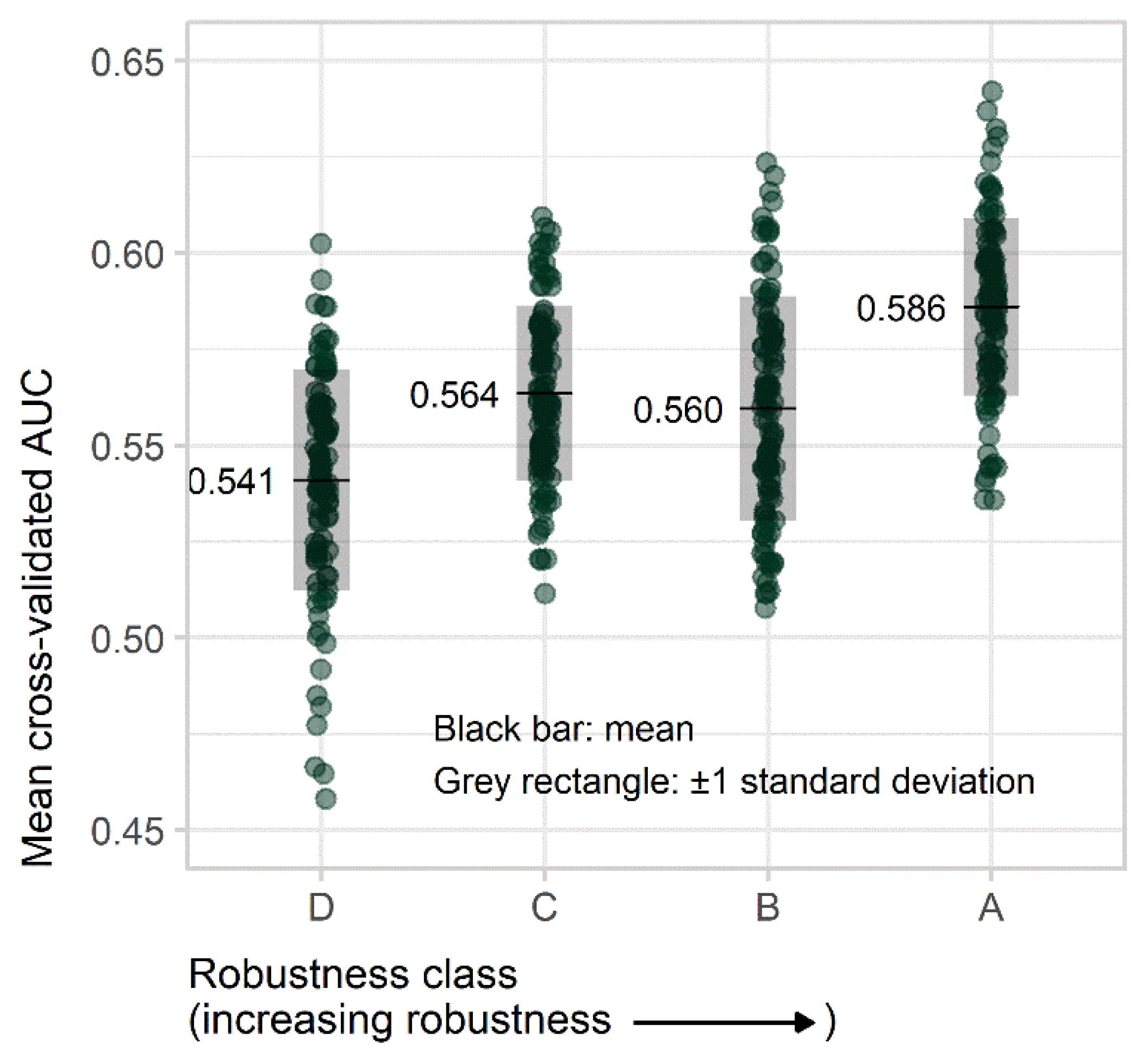
| Robustness Class | CMV Range (Mean) | AUC Mean (SD) | Coefficient (95% CI) | Standard Error | p-Value * |
|---|---|---|---|---|---|
| D | 0.47–1.43 (0.97) | 0.54 (0.029) | Reference | ||
| C | 0.19–0.46 (0.30) | 0.56 (0.023) | 0.022 (0.015–0.030) | 0.004 | <0.005 |
| B | 0.14–0.19 (0.16) | 0.56 (0.029) | 0.018 (0.011–0.026) | 0.004 | <0.005 |
| A | 0.020–0.14 (0.089) | 0.59 (0.023) | 0.045 (0.038–0.052) | 0.004 | <0.005 |
Publisher’s Note: MDPI stays neutral with regard to jurisdictional claims in published maps and institutional affiliations. |
© 2021 by the authors. Licensee MDPI, Basel, Switzerland. This article is an open access article distributed under the terms and conditions of the Creative Commons Attribution (CC BY) license (https://creativecommons.org/licenses/by/4.0/).
Share and Cite
Acciavatti, R.J.; Cohen, E.A.; Maghsoudi, O.H.; Gastounioti, A.; Pantalone, L.; Hsieh, M.-K.; Conant, E.F.; Scott, C.G.; Winham, S.J.; Kerlikowske, K.; et al. Incorporating Robustness to Imaging Physics into Radiomic Feature Selection for Breast Cancer Risk Estimation. Cancers 2021, 13, 5497. https://doi.org/10.3390/cancers13215497
Acciavatti RJ, Cohen EA, Maghsoudi OH, Gastounioti A, Pantalone L, Hsieh M-K, Conant EF, Scott CG, Winham SJ, Kerlikowske K, et al. Incorporating Robustness to Imaging Physics into Radiomic Feature Selection for Breast Cancer Risk Estimation. Cancers. 2021; 13(21):5497. https://doi.org/10.3390/cancers13215497
Chicago/Turabian StyleAcciavatti, Raymond J., Eric A. Cohen, Omid Haji Maghsoudi, Aimilia Gastounioti, Lauren Pantalone, Meng-Kang Hsieh, Emily F. Conant, Christopher G. Scott, Stacey J. Winham, Karla Kerlikowske, and et al. 2021. "Incorporating Robustness to Imaging Physics into Radiomic Feature Selection for Breast Cancer Risk Estimation" Cancers 13, no. 21: 5497. https://doi.org/10.3390/cancers13215497