

A Method to Compute Shadow Geometry in Open Building Information Modeling Authoring Tools: Automation of Solar Regulation Checking

Laboratoire Piment, Université de La Réunion, 120 Avenue Raymond Barre, 97430 Le Tampon, France
*
Author to whom correspondence should be addressed.
Buildings 2023, 13(12), 3120; https://doi.org/10.3390/buildings13123120
Submission received: 20 November 2023
/
Revised: 11 December 2023
/
Accepted: 12 December 2023
/
Published: 15 December 2023
(This article belongs to the Topic Sustainability, Challenges and Opportunities to Optimizing Building Performance)
Abstract
:Building solar protection regulations is essential to save energy in hot climates. The protection performance is assessed using a shading factor computation that models the sky irradiance and the geometry of shadow obstructing the surface of interest. While Building Information Modeling is nowadays a standard approach for practitioners, computing shadow geometry in BIM authoring tools is natively impossible. Methods to compute shadow geometry exist but are out of reach for the usual BIM authoring tool user because of algorithm complexity and non-friendly BIM implementation platform. This study presents a novel approach, dubbed solid clipping, to calculate shadow geometry accurately in a BIM authoring tool. The aim is to enhance project delivery by enabling solar control verification. This method is based on typical Computer Aided Design (CAD) in BIM authoring tools. The method is generic enough to be implemented using any BIM authoring tool’s visual and textual API. This work demonstrates that a thermal regulation, here the French overseas one, can be checked concerning solar protection, thanks to a BIM model. Beyond automation, this paper shows that, by directly leveraging the BIM model, designs presently not feasible by the usual process can be studied and checked.
1. Introduction
The incorporation of renewable energy sources is essential for attaining enduring sustainability [1]. Limitless solar energy is necessary to mitigate the construction sector’s greenhouse gas (GHG) emissions [2]. There are two methods for converting radiative energy. The first is thermal transfer, where the energy is used for heating purposes or to generate hot water by passing it through the building envelope. The other method involves the absorption of solar radiation by solar panels, which then convert it into electric energy using photovoltaic (PV) systems [3]. Optimizing both conversion systems is crucial to achieving optimal performance throughout the seasons, particularly in tropical climates [4,5,6]. It is essential to consider the unique characteristics of each building, like shadows. Considering shadows is crucial to guarantee the dependable functioning of systems. While building designers may prioritize assessing the overall performance of a structure, such as energy consumption per square meter, they can also utilize more minor scale performance indicators, such as the shading factor, to evaluate specific components. This factor quantifies the proportion of energy that reaches the glass surface of a window, taking into account any potential barrier caused by the surrounding environment, compared to the energy that comes to the surface without any obstruction. Subsequently, it can be employed, specifically in regions with tropical climates, to assess the efficacy of shade devices. Similarly to the regulations followed in Indonesia and India [7], the French regulation for tropical climate (RTAADOM) presents a parametric model and tables of acceptable values for determining the shading factor of some building components such as walls or windows. These values are contingent upon the location of the building and the orientation of the windows [8,9,10,11].
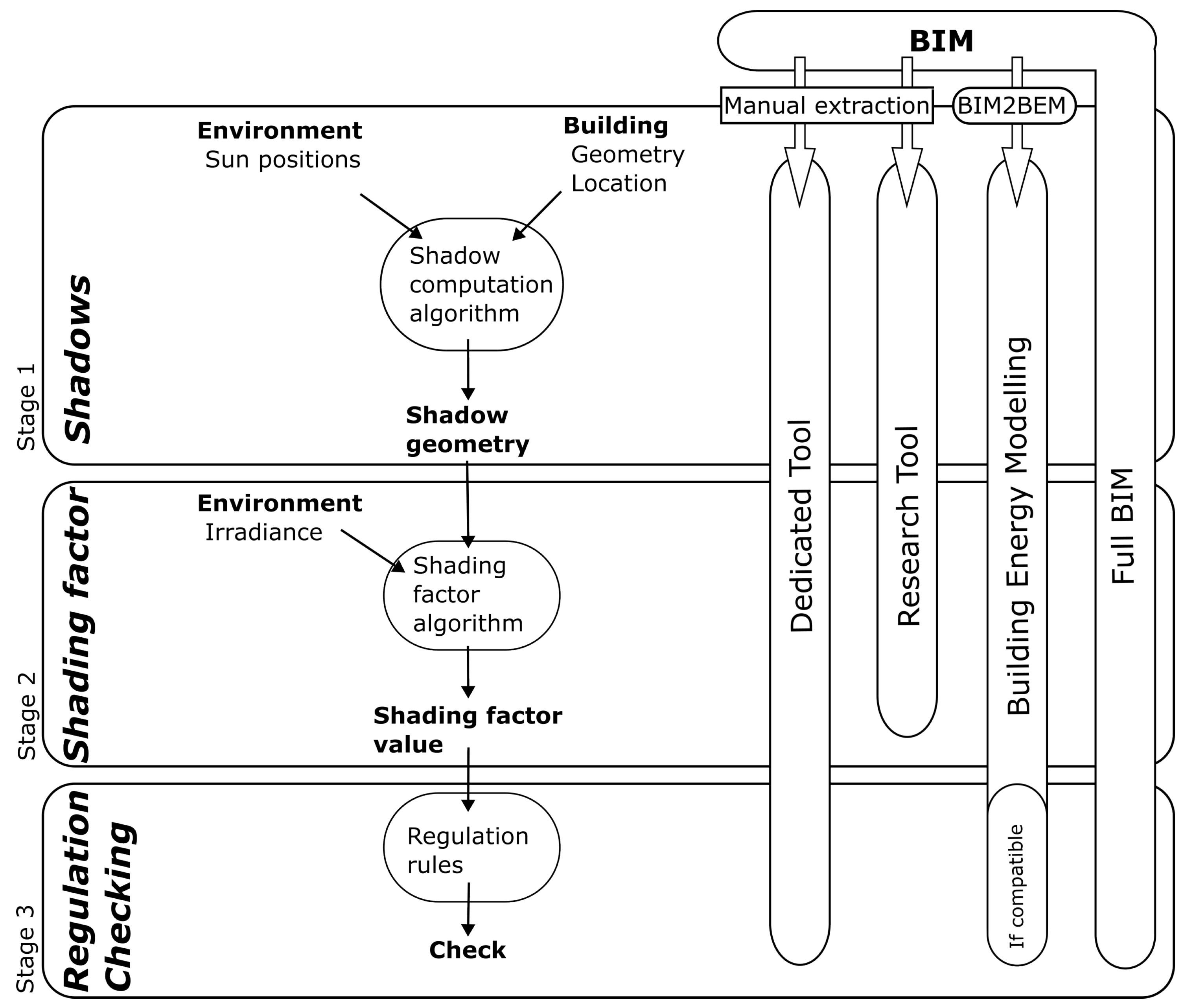
Figure 1 shows the framework of this paper. The left part of the figure illustrates this point of view and highlights each stage’s important input and output. The right part shows different implementation alternatives regarding the computation stages. The left part of Figure 1 shows that regulation based on the shading factor relies on three stages: (1) evaluation of shadow geometric features such as area, (2) integration in a shading factor model to compute the value of shading factor, and, finally, (3) comparison to a reference value to check a regulation. This paper focuses on this framework of regulation checking thanks to a shading factor. While the second stage is nowadays straightforward, thanks to accessible numerical tools such as a spreadsheet or a scripting language, the computation of 3D shadow geometry features (first stage) remains a challenging task.
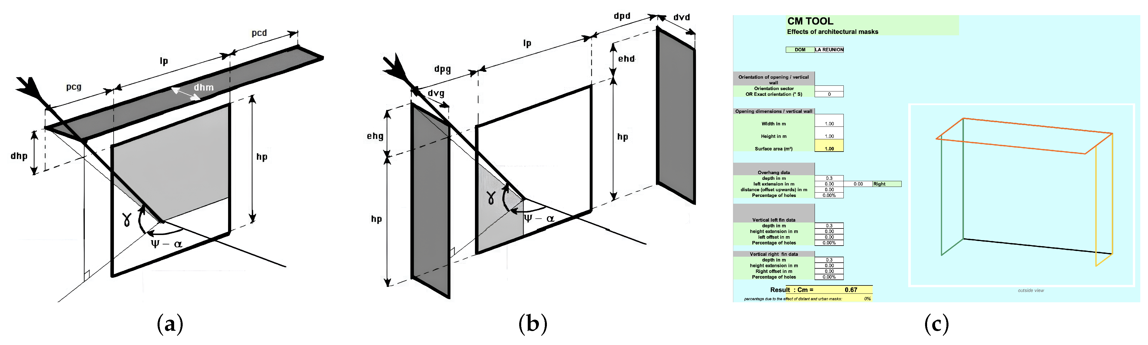
The RTAADOM offers a specialized tool in a secure spreadsheet that combines all steps necessary to calculate shading factor values. The system utilizes a basic parametric geometric model of solar protection, requiring the user to manually map their building design onto the parameter space of the geometric model. Figure 2 shows both the geometric configurations modeled in the RTAADOM and a snapshot of the user interface. Figure 2a shows all the parameters used to parametrize the overhang protection. If vertical fins are added, Figure 2b shows all the supplementary parameters to parametrize them. The official and protected spreadsheet that implements this model can be found on the French government website [12] and a snapshot of the interface is shown in Figure 2c. While the user directly inputs most parameters to describe the solar protection geometry, the parameters and correspond to the sun’s position in the computation and are not exposed to the user. Real designs are generally more complex than the geometric model and the projection represents a critical step in the process. To overcome this point, in other words, to compute the shading factor with complex geometry, two alternative approaches are identified. The first one is to use research tools that implement various approaches over the first two stages of the process. While very flexible and capable thanks to cutting-edge algorithms, by design, its purpose is not oriented through checking and relies on tailored inputs.
Designers can use Building Energy Modeling (BEM) approaches and established and reliable tools like EnergyPlus. EnergyPlus incorporates a shading factor as an intermediate outcome in the overall performance assessment. Proficiency in software development is necessary to make any adjustments to this implementation based on many modeling assumptions. Therefore, it is essential to ensure that the shading factor used in BEM matches the one used in the software. Nevertheless, this alignment needs to be more consistently apparent, as exemplified by the instance of RTAADOM. Integrating Building Information Modeling (BIM) into building performance modeling is a significant step in sustainable design. This collaboration enhances the ability to use parametric design, allowing architects and engineers to quickly evaluate multiple potential solutions, leading to more knowledgeable and effective decision-making processes [13]. In addition, the seamless integration of BIM with building rating systems can transform the green certification process by automating several components and enhancing a building’s sustainability credentials. The BIM approach, known for extracting material quantities from models automatically, makes green building assessments easier and faster by expediting sustainability evaluations [14,15]. Furthermore, integrating BIM into evaluations of environmentally friendly construction dramatically improves project completion efficiency and data organization while supporting sustainability goals. BIM also has a crucial function in optimizing the efficiency of regulatory compliance and certification procedures. An example is the emphasized advantages of integrating Building Information Modeling (BIM) with energy simulation as part of the LEED certification procedure [16]. Nevertheless, exporting the BIM model amplifies the likelihood of flaws inside the file, which could compromise the outcomes’ precision. Another method involves directly processing BIM model data within the modeling software to avoid any data loss, although this necessitates using proprietary software. To tackle more extensive issues related to accessibility, some authors have proposed using tools that rely on the IFC format. The utilization of IFC files simplifies the implementation of external tools, especially in cloud environments. An instance of a BIM platform that operates in the cloud and includes a calculation tool to verify the Envelope Thermal Transfer Value (ETTV) calculation showcases the potential of this technique to improve accessibility and scalability while guaranteeing the precision of essential calculations [17].
Nowadays, Building Information Modeling (BIM) workflow and associated authoring tools have become standard practice in designing buildings. Beyond software, BIM is a way to structure and efficiently share the building data’s complexity. Over the last two decades, the Industry Foundation Classes (IFC) data scheme has become the standard for open BIM. The Industry Foundation Classes (IFC) file format is a crucial Building Information Modeling (BIM) standard. IFC, developed by BuildingSMART, aims to enhance interoperability within the architectural, engineering, and construction (AEC) sector. The open data model, compliant with the Standard [18], facilitates the transfer and dissemination of information often utilized in BIM workflows, surpassing the constraints imposed by proprietary software. An IFC file is a complete data container containing detailed metadata and geometric information about building elements. The file format encompasses specific information such as the geometric depiction, material characteristics, and spatial connections of building elements. It facilitates interoperability in AEC but true interoperability between BIM software using IFC has not been achieved. Nonetheless, based on open or closed data schema, BIM authoring tools should be the original source of information to compute the shading factor. In other words, the inputs of the three previously presented approaches (Dedicated Tool, Research Tool, and BEM) should be extracted and/or converted from BIM to a suitable data format. Due to their specificity, manual extraction prevails for the first two. Concerning BEM, automating the generation of the BEM model from BIM data is an active topic of research [19] but remains challenging due to the complexity of both data models. Even if automation works, the benefits of BIM workflow could be limited by any data flow without automatic feedback from BEM to BIM. To overcome that challenge, a solution is to embrace a total BIM approach where the needed shading factor is computed using a BIM authoring tool with native data. This is the primary goal of this paper.
The primary obstacle lies in calculating the shadow geometry, specifically within a BIM authoring tool. Although they may be seen, they lack practicality and must be recalculated as simple geometric entities. This research introduces a novel technique dubbed “solid clipping” that utilizes common elements of the Computer Aided Design (CAD) kernel found in BIM authoring tools. The method is easily comprehensible and uncomplicated to execute with either a visual or textual API. This paper demonstrates implementing a technique in openBIM using IFCOpenshell and Python. The method is then employed to calculate the RTAADOM shading factor in a BIM model. The results of the geometric reference model are discussed.
This paper is structured as follows. Section 2.1 provides information regarding the calculation of the shading factor, encompassing both Stage 1 and Stage 2. Section 2.2 entails an exposition of the solid clipping technique. Section 3 covers applying solid clipping to calculate the RTAADOM shading factor in BIM.
2. Methodology
This section provides a brief state of the art about the computation of shading factor. It also introduces the shading factor used in the RTAADOM that has to be checked on the BIM model. A new method to compute the BIM authoring tool’s shadow geometry easily is introduced.
2.1. An Overview of Shading Factor Computation
2.1.1. Shadow Geometry Computation
Computation of shadow is a mature field in video games, virtual reality, and 3D modeling. Over the last few decades, numerous techniques have been created to, most of the time, render better and faster [20], in other words, to optimize software and hardware to achieve realistic views for human eyes through pixels. The goal here is different. It is to compute the geometry of the direct shadow of a single light source for quantitative analysis needed in design and engineering. Unfortunately, standard BIM authoring tools or viewers compute and display such shadows but do not expose them as actionable objects for quantitative analysis. Intuitively, lighting simulation software would be a perfect candidate to compute shadow. Still, most of the effort is oriented to rendering a realistic view and predicting lighting conditions inside buildings [21,22,23,24]. Moreover, direct shadow geometries are intermediate and unreachable computation results as a step of a building energy analysis workflow. In the same way, direct shadows are an intermediate result of Building Environmental Modeling (BEM) based on zone model [25]. Beyond the expertise needed to extract such results, these modeling approaches need to convert and augment BIM data to a suitable dedicated model [26,27,28]. Even if progress has been made in this task, the cost and expertise needed to build such a model to extract shadow are disproportionate.
In the context of solar radiation modeling, shadow computation methods can be classified into four categories: trigonometric (TgM), polygon clipping (PgC), pixel counting (PxC), and ray tracing (RT). Trigonometric models use parametric geometry of obstructions to analytically project them on the surface of interest [29]. While computationally efficient, they are limited in terms of geometry [30]. The French regulation RTAADOM proposes such a model, implemented in a spreadsheet, to compute the shading factor for a parametric model of solar protection [31]. Polygon clipping (PgC) computes shadow as the intersection of polygons on the surface of interest [32]. The polygons are the projection of the faces of obstructing objects. This method is much more versatile but shows limitations with non-convex or holed shapes in standard implementations [33]. Despite these limitations, PgC is primarily implemented in the BEM tools. Pixel counting computes the number of lighted (oppositely shaded) pixels representing the surface of interest from the sun’s viewpoint. While this method provides an estimation due to sampling through pixels, it is versatile and precise [33,34] thanks to modern graphic hardware that can efficiently deal with high-resolution images. In order to achieve optimal results, it is necessary to apply this technique using a visual programming language like OpenGL, which consequently demands specialized expertise. Ray tracing involves the casting and propagating of numerous basic rays that eventually undergo reflection [35,36,37]. In the forward version, the rays are cast from the sun and those that hit the surface of interest can be used to evaluate the shadow area. In the backward version, the rays are cast from the surface of interest and the counts of the number of rays intercepted by the obstruction can be used to estimate shadows. As a sampling method based on randomness, precision should assessed [38]. One significant advantage is that the multireflection of rays can be modeled.
2.1.2. Shading Factor
For a given surface, the shading factor describes the ratio between incoming irradiance with obstruction and irradiance without I. The shading factor comprises two models: a sky model to describe the different irradiance components caught by a surface of interest and a shadow model to compute the shaded area. The sky model generally decomposes the total irradiance into direct, diffuse, and reflected components, and projects it on a tilted surface. The shadow model describes how each irradiance component is impacted by obstructions in front of the surface of interest.
Sky model decomposes the total irradiance I on a tilted surface in the direct and the diffuse ones for a given location and time on earth. Numerous models have been developed [39], varying in terms of physical and mathematical complexity to offer better precision in predictions [40]. Models mainly differ in how they decompose the diffuse component into different contributions: isotropic from the sky dome, circumsolar, horizon brightening, and reflected from the ground.
This work will only use a basic model with isotropic diffuse radiation for both sky and ground [41,42]. Such a model allows us to consider essential physical traits of the problem without much mathematical complexity. Moreover, the thermal regulation that has to be checked automatically is based on this model. The total irradiance I is then written as with:
where is the direct-normal component of solar irradiance on the horizontal surface, is a geometric factor, is the global diffuse horizontal solar irradiance, is the tilt angle of the surface from the horizon, is the global horizontal solar irradiance, and is the soil albedo.
To compute a shading factor, including diffused irradiance, one needs to consider the effect of shadow on diffuse component . One common approach is to consider the non-direct source of radiance as a sum of direct sources from different directions with associated direct shadows. In other words, the shaded diffuse component is computed via the integration of discretized shaded sources [30,32,40,43]. Following [29], the instantaneous shading factor is defined for one solar position by the ratio between the irradiance with shadow and without:
where , , and are the geometric shading factors for direct, diffuse, and reflected irradiance components, respectively. For direct irradiance, is given by the ratio of the sunlit area and its total area: . For diffuse component and a given hemisphere discretization, is given by:
where i and j denote the discretized height and latitude coordinates of the considered portion of sky hemisphere, is the radiance passing through the portion of hemisphere calculated according a sky model, is the angle between the sky element and the normal of the surface, and is the solid angle of the sky portion seen from the surface. A similar approach can compute a geometric shading ratio for the reflected component depending on the use case and the modeling hypothesis about ray reflection. While the instantaneous shading factor can be interesting to assess predictions minutely, the average overtime period is often used in application, . Alternatively, the RTAADOM uses an integral form to define the shading factor:
2.2. A New Method to Compute Shadow Geometry: Solid Clipping
BIM authoring tools generally implement a Computer Aided Design (CAD) kernel suitable to model the shapes of building components using surface and solid modeling. The proposed method is based on essential solid modeling operations such as extrusion and intersection to compute shadow, inspired by the polygon clipping approach. It is an oversimplified version of the shadow volume technique [44], a well-known method capable of rendering complex scenes in terms of geometry and daylighting. Indeed, our goal is to compute shadow on one face F of the model for a unique direct light source.
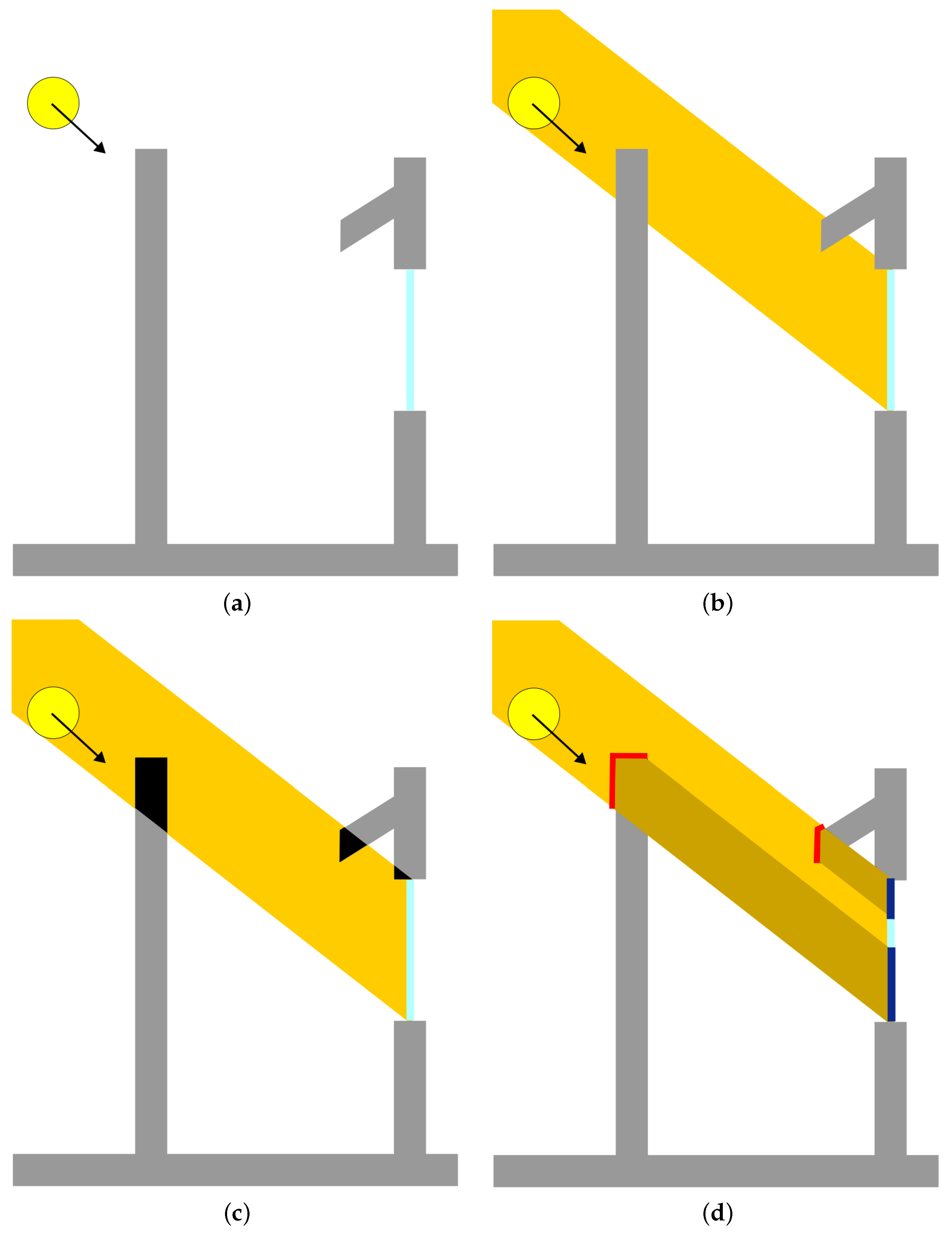
As it can be seen in Figure 3, where the method is applied to cast shadows on a window, the shadow computation method consists of four steps:
- Identification of the building walls or elements that can cast a shadow regarding sun exposition, as in Figure 3a;
- Extrusion of a three-dimensional (3D) sun path in the direction of the wall where shadows have to be evaluated, as in Figure 3b;
- Calculation of 3D intersections of the sun path with the building to identify the parts that can generate shadows on the considered walls, as in Figure 3c;
- Extrusion of previous 3D intersections, reduced to intersection surfaces, up to the considered walls to trace and calculate the shadows, as in Figure 3d.
This method has inspired the algorithm described in Algorithm 1.
| Algorithm 1: Algorithm to compute shadow |
 |
Let us detail line by line Algorithm 1 along with a 2D illustration in Figure 3. The extension to 3D is straightforward.
- Line 1
- The points downward, i.e., from the sun through the face of interest F. F is extruded to the infinite along to create the “solid of light” . It represents the light flux without obstruction, as shown in Figure 3a.
- Line 2
- The Boolean intersection between the solid and all the other solid of the BIM model () is computed and stored in . Shown in black in Figure 3c.
- Line 5 to 8
- Line 10
- The Boolean union of all the (dark blue in Figure 3d) defines the face shadow .
The order of solid operation has been optimized to propose a robust algorithm. Indeed, one can think of uniting the extrusion to perform one unique intersection, thus saving time. It has been found that the intersection of a unique volume resulting from the union of multiple possibly overlapping extrusions is more error-prone than the union of multiple intersections on the face F. In other words, for the sake of robustness, it is better to deal with the most straightforward atomic geometry. The advantages and limitations of this method regarding application results will be discussed at the end of the paper.
3. Application: Checking the RTAADOM on BIM Models
The solid clipping method has been applied to compute the RTAADOM shading factor. Thanks to the IFCOpenShell library, a Python tool has been developed to implement the solid clipping method to compute the RTAADOM shading factor .
Validation of RTAADOM Shading Factor Computed Using BIM
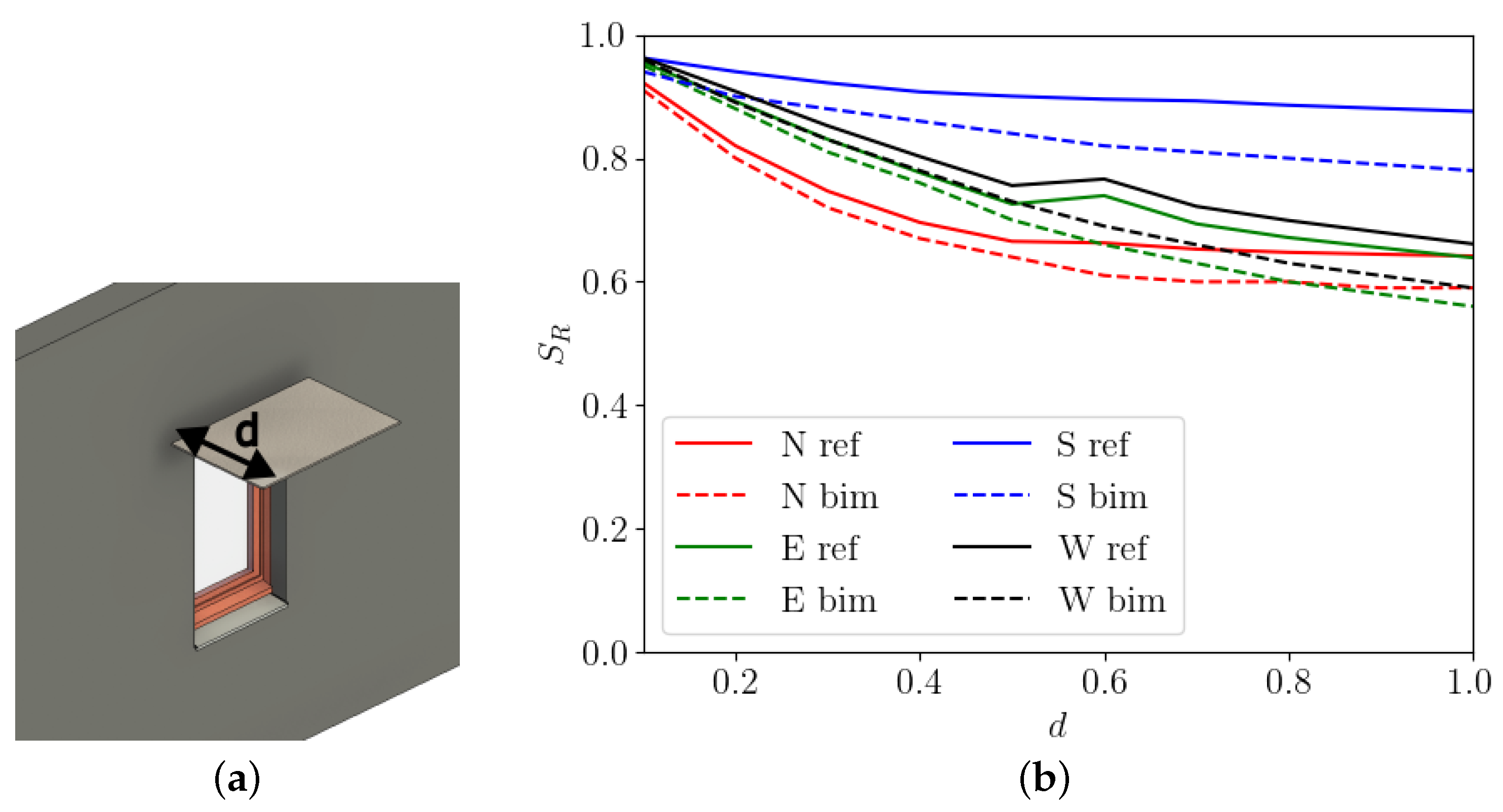
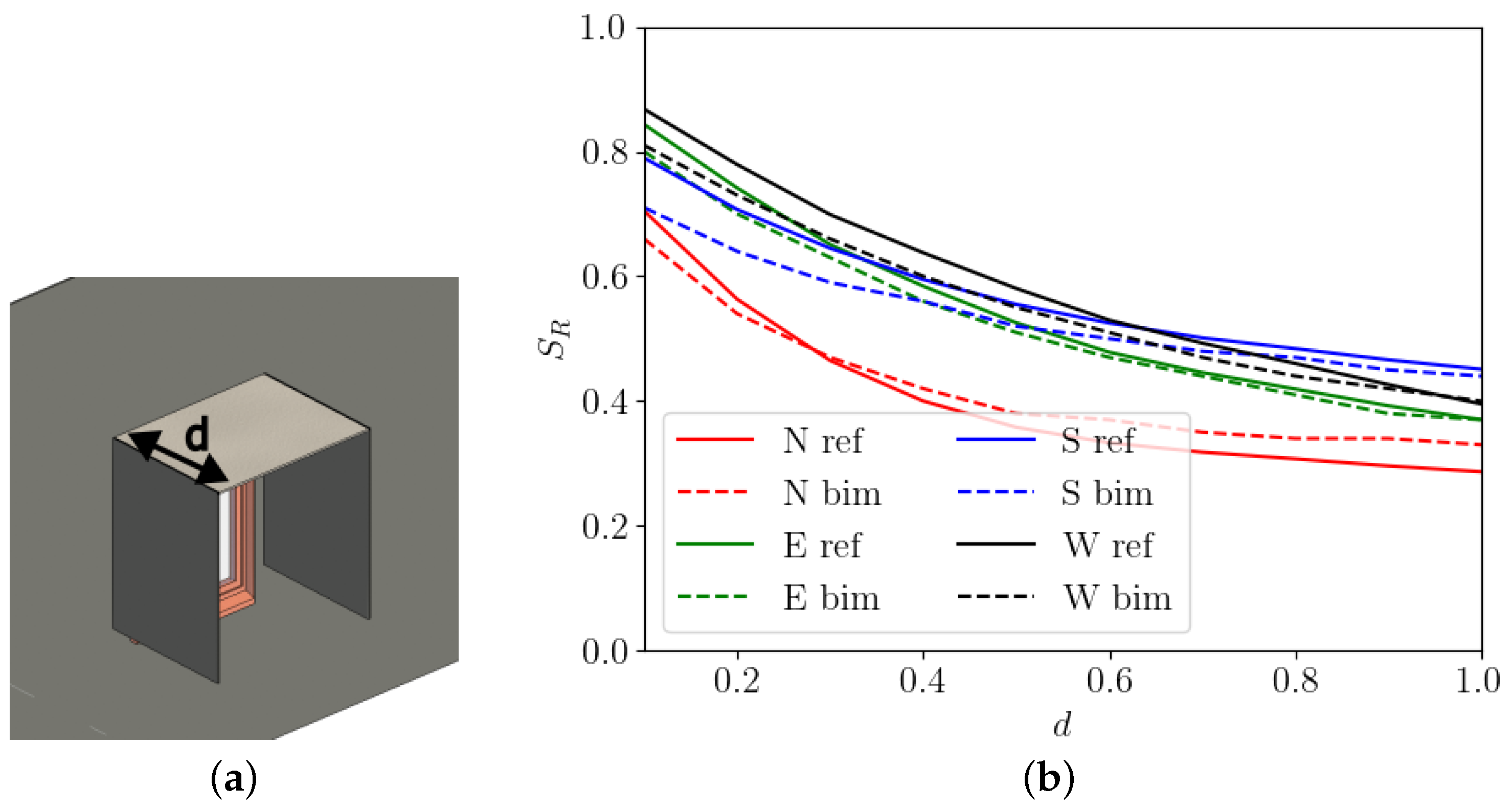
In this section, a comparison of shading factor values given by the RTAADOM official Excel sheet with those computed using our automatic analysis of an IFC file has been made. Varying window configuration regarding protection geometry and orientation, values were quantitatively compared. The first model comprises four walls and 10 identical windows with solar protection hosted on the same linear wall. An overhang of different depths is associated with each window, as shown in Figure 4a. For each window, the overhang depth d increases from to by steps. This BIM model, and thus these 10 protection configurations, are strictly geometrically equivalent to those managed by the parametric model of the RTAADOM (see Figure 2).
The window’s orientation can be controlled by setting the angle between the project north and the true north. The comparison of the values for a window oriented to the four cardinal orientations can be achieved.
Figure 4b shows values as a function of for four orientations. Table 1 shows the corresponding raw data. The solid line represents values computed from the IFC file with solid clipping and the dashed lines correspond to the values given by the regulation Excel tool . As expected, decreases as increases. Except for the south orientation, there is an excellent agreement between and values.
A second model was created by adding vertical fins to each overhang, as shown in Figure 5a. Table 2 shows the corresponding raw data. Figure 5b shows an even better agreement between and when vertical fins are added.
Table 3 shows the Mean Absolute Error (MAE) for each orientation and protection configuration. The MAE is below five percent except for the overhang facing south. Merging all the data, MAE is equal to . The raw data can be found in Table 1 and Table 2. The discrepancy can be attributed to the modeling of the diffuse part. While the RTAADOM gives an explicit formula, our implementation requires an integration process sensitive to many parameters. Nonetheless, the results are very close and such small errors should be balanced by the automation gain, both in time and quality.
4. Conclusions and Perspectives
This paper introduces a new method to compute the exact shadow geometry necessary to evaluate shading factors. This method, called solid clipping, uses simple computational geometry tools implemented in BIM authoring tools and actionable through textual or visual API. Implementing the shading factor with a reference tool associated with French regulation has been validated. It has also been qualitatively shown that the design is unverifiable with the regulation and can be easily checked with our implementation. From an engineering perspective, two main benefits can be identified. Firstly, proper automation makes the cost of regulation checking plummet. Thus, checking a regulation becomes a quality assessment tool throughout the whole life of the project not just at the end. Secondly, implementing solid clipping using the BIM API allows us to deal with the geometry of shadows as complex as those of the building elements that generate them. In other words, if a solar protection design is created with a BIM authoring tool, the generated shadow can be leveraged to compute a shading factor. Combining these benefits will lead to a better cost–quality–delay balance in delivering sustainable buildings designed in BIM.
4.1. Extending Regulation Using BIM
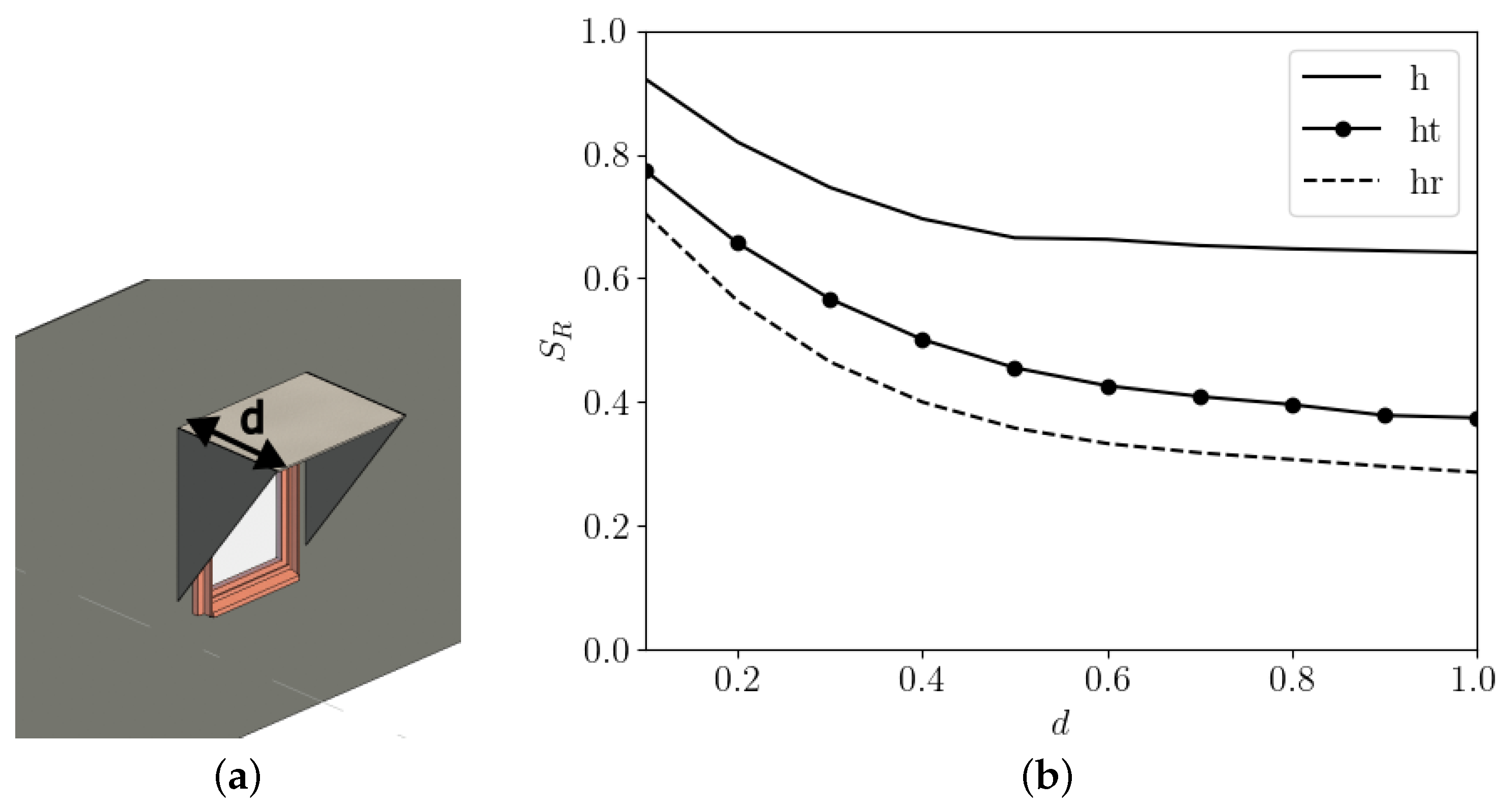
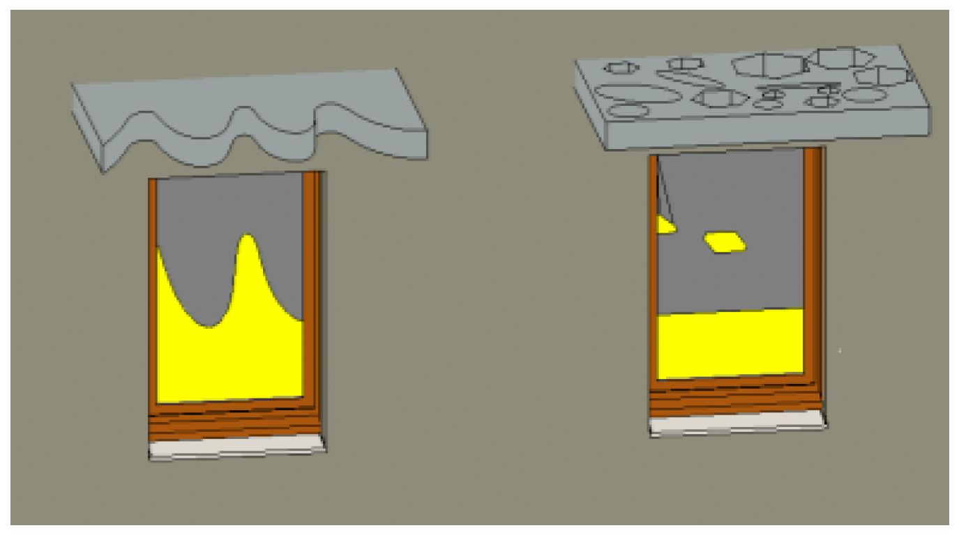
Having assessed the precision and thus validated the implementation of shading factors, it is possible to extrapolate the computation to a configuration not handled by the regulation. So, was computed for protection with triangle-shaped fins instead of rectangular ones. Intuitively, this is an intermediate solution in terms of performance between the previously studied configurations: overhang with and without rectangular fins. Figure 6b confirms this by showing for the three studied protection configurations. As expected, the triangle-shaped fins generate intermediate values of . Beyond such a design as is currently implemented in the tropical French territory, the original and creative design can be assessed usingour method. For example, Figure 7 shows three examples of the solar protection of different architectural complexity for illustration. While inefficient, they highlight the capability of the solid clipping method to deal with complex geometries.
4.2. Research Directions
From a research perspective, this work paves the way in multiple directions. For example, advanced components such as phase-changing material or thermochromic glasses are exposed to non-uniform irradiance on their surface. Having easy access to realistic shadow geometries thanks to solid clipping and BIM modeling will improve models and thus their deployment for energy saving. More broadly, such exact and potentially complex shadows can be used as an input table in BEM tools to assess the impact of advanced solar protection. Smart solar protection could also use precise knowledge of shadow geometry. Indeed, having an internal reference in addition to sensors could help smart systems make better decisions and detect faults.
Author Contributions
Conceptualization, C.V., D.B. and G.R.; Methodology, C.V. and D.B.; Software, C.V.; Validation, C.V.; Formal analysis, C.V.; Investigation, C.V. and D.B.; Resources, C.V.; Data curation, C.V.; Writing—original draft, C.V., D.B. and G.R.; Writing—review & editing, C.V., D.B. and G.R.; Visualization, C.V.; Project administration, G.R.; Funding acquisition, G.R. All authors have read and agreed to the published version of the manuscript.
Funding
This research was funded by the French Deposits and Consignments Office grant number Fund: PIA3-MCENT.
Data Availability Statement
The data presented in this study are available in the article.
Conflicts of Interest
The authors declare no conflict of interest.
References
- Ang, T.Z.; Salem, M.; Kamarol, M.; Das, H.S.; Nazari, M.A.; Prabaharan, N. A comprehensive study of renewable energy sources: Classifications, challenges and suggestions. Energy Strategy Rev. 2022, 43, 100939. [Google Scholar] [CrossRef]
- Li, G.; Li, M.; Taylor, R.; Hao, Y.; Besagni, G.; Markides, C. Solar energy utilisation: Current status and roll-out potential. Appl. Therm. Eng. 2022, 209, 118285. [Google Scholar] [CrossRef]
- Hayat, M.B.; Ali, D.; Monyake, K.C.; Alagha, L.; Ahmed, N. Solar energy-A look into power generation, challenges, and a solar-powered future. Int. J. Energy Res. 2019, 43, 1049–1067. [Google Scholar] [CrossRef]
- Vassiliades, C.; Agathokleous, R.; Barone, G.; Forzano, C.; Giuzio, G.; Palombo, A.; Buonomano, A.; Kalogirou, S. Building integration of active solar energy systems: A review of geometrical and architectural characteristics. Renew. Sustain. Energy Rev. 2022, 164, 112482. [Google Scholar] [CrossRef]
- Rabani, M.; Bayera Madessa, H.; Nord, N. Achieving zero-energy building performance with thermal and visual comfort enhancement through optimization of fenestration, envelope, shading device, and energy supply system. Sustain. Energy Technol. Assessments 2021, 44, 101020. [Google Scholar] [CrossRef]
- Hwang, R.L.; Chen, W.A. Identifying relative importance of solar design determinants on office building façade for cooling loads and thermal comfort in hot-humid climates. Build. Environ. 2022, 226, 109684. [Google Scholar] [CrossRef]
- Bhatia, A.; Sangireddy, S.A.R.; Garg, V. An approach to calculate the equivalent solar heat gain coefficient of glass windows with fixed and dynamic shading in tropical climates. J. Build. Eng. 2019, 22, 90–100. [Google Scholar] [CrossRef]
- Grosdemouge, V.; Garde, F. Passive design in tropical climates: Key strategies implemented in a French certified sustainable neighbourhood. In Proceedings of the PLEA 2016 Los Angeles—36th International Conference on Passive and Low Energy Architecture, Los Angeles, CA, USA, 11–13 July 2016. [Google Scholar]
- Garde, F.; Adelard, L.; Boyer, H.; Rat, C. Implementation and experimental survey of passive design specifications used in new low-cost housing under tropical climates. Energy Build. 2004, 36, 353–366. [Google Scholar] [CrossRef]
- Garde, F.; David, M.; Adelard, L.; Ottenwelter, E. Elaboration of thermal standards for french tropical islands. Presentation of the PERENE Project. In Proceedings of the CLIMA International Conference in the Field of Heating, Ventilation and Airconditioning (HVAC), Lausanne, Switzerland, 9–12 October 2005; pp. 71–83. [Google Scholar]
- Garde, F.; Ottenwelter, E.; Bornarel, A. Integrated building design in tropical climates: Lessons learned from the ENERPOS net zero energy building. ASHRAE Trans. 2012, 118, 1–9. [Google Scholar]
- Textes réglementaires et fiches d’application de la RTAADOM. Available online: https://www.reunion.developpement-durable.gouv.fr/textes-reglementaires-et-fiches-d-application-a686.html (accessed on 11 December 2023).
- Casini, M. Chapter 5—Building performance simulation tools. In Construction 4.0; Woodhead Publishing: Sawston, UK, 2021; pp. 221–262. [Google Scholar]
- Seghier, T.E.; Khosakitchalert, C.; Lim, Y.W. A BIM-Based Method to Automate Material and Resources Assessment for the Green Building Index (GBI) Criteria. In Proceedings of 2021 4th International Conference on Civil Engineering and Architecture; Springer: Singapore, 2022; pp. 527–536. [Google Scholar]
- Marzouk, M.; Ayman, R.; Alwan, Z.; Elshaboury, N. Green building system integration into project delivery utilising BIM. Environ. Dev. Sustain. 2022, 24, 6467–6480. [Google Scholar] [CrossRef]
- Ryu, H.S.; Park, K.S. A study on the LEED energy simulation process using BIM. Sustainability 2016, 8, 138. [Google Scholar] [CrossRef]
- Liu, Z.; Wang, Q.; Gan, V.J.; Peh, L. Envelope thermal performance analysis based on building information model (BIM) cloud platform—Proposed green mark collaboration environment. Energies 2020, 13, 586. [Google Scholar] [CrossRef]
- 16739-1:2018; Industry Foundation Classes (IFC) for Data Sharing in the Construction and Facility Management Industries—Part 1: Data Schema. International Organisation For Standardisation: Geneva, Switzerland, 2018.
- Ciccozzi, A.; de Rubeis, T.; Paoletti, D.; Ambrosini, D. BIM to BEM for Building Energy Analysis: A Review of Interoperability Strategies. Energies 2023, 16, 7845. [Google Scholar] [CrossRef]
- Akenine-Möller, T.; Haines, E.; Hoffman, N. Real-Time Rendering; CRC Press: Boca Raton, FL, USA, 2019. [Google Scholar]
- Tzempelikos, A.; Athienitis, A.K. The impact of shading design and control on building cooling and lighting demand. Sol. Energy 2007, 81, 369–382. [Google Scholar] [CrossRef]
- Montiel-Santiago, F.J.; Hermoso-Orzáez, M.J.; Terrados-Cepeda, J. Sustainability and Energy Efficiency: BIM 6D. Study of the BIM Methodology Applied to Hospital Buildings. Value of Interior Lighting and Daylight in Energy Simulation. Sustainability 2020, 12, 5731. [Google Scholar] [CrossRef]
- Shikder, S.H.; Price, A.; Mourshed, M. Evaluation of four artificial lighting simulation tools with virtual building reference. In Proceedings of the European Simulation and Modelling Conference (ESM 2009), Leicester, UK, 28–29 October 2009; pp. 77–82. [Google Scholar]
- Natephra, W.; Motamedi, A.; Fukuda, T.; Yabuki, N. Integrating building information modeling and virtual reality development engines for building indoor lighting design. Vis. Eng. 2017, 5, 19. [Google Scholar] [CrossRef]
- Shin, M.; Haberl, J.S. Thermal zoning for building HVAC design and energy simulation: A literature review. Energy Build. 2019, 203, 109429. [Google Scholar] [CrossRef]
- Gao, H.; Koch, C.; Wu, Y. Building information modelling based building energy modelling: A review. Appl. Energy 2019, 238, 320–343. [Google Scholar] [CrossRef]
- Sun, Y.; Haghighat, F.; Fung, B.C.M. A review of the-state-of-the-art in data-driven approaches for building energy prediction. Energy Build. 2020, 221, 110022. [Google Scholar] [CrossRef]
- Farzaneh, A.; Monfet, D.; Forgues, D. Review of using Building Information Modeling for building energy modeling during the design process. J. Build. Eng. 2019, 23, 127–135. [Google Scholar] [CrossRef]
- Cascone, Y.; Corrado, V.; Serra, V. Calculation procedure of the shading factor under complex boundary conditions. Sol. Energy 2011, 85, 2524–2539. [Google Scholar] [CrossRef]
- Elmalky, A.M.; Araji, M.T. Computational procedure of solar irradiation: A new approach for high performance façades with experimental validation. Energy Build. 2023, 298, 113491. [Google Scholar] [CrossRef]
- Outil de Calcul du Coefficient, Cm. Available online: https://rt-re-batiment.developpement-durable.gouv.fr/IMG/zip/outil_cm_v1.0.xls.zip (accessed on 29 November 2023).
- Melo, E.G.; Almeida, M.P.; Zilles, R.; Grimoni, J.A. Using a shading matrix to estimate the shading factor and the irradiation in a three-dimensional model of a receiving surface in an urban environment. Sol. Energy 2013, 92, 15–25. [Google Scholar] [CrossRef]
- Rocha, A.P.d.A.; Oliveira, R.C.; Mendes, N. Experimental validation and comparison of direct solar shading calculations within building energy simulation tools: Polygon clipping and pixel counting techniques. Sol. Energy 2017, 158, 462–473. [Google Scholar] [CrossRef]
- Rocha, A.P.d.A.; Mendes, N.; Oliveira, R.C.L.F. Domus method for predicting sunlit areas on interior surfaces. Ambiente Construído 2018, 18, 83–95. [Google Scholar] [CrossRef]
- Wang, X.; Zhang, X.; Zhu, S.; Ren, J.; Causone, F.; Ye, Y.; Jin, X.; Zhou, X.; Shi, X. A novel and efficient method for calculating beam shadows on exterior surfaces of buildings in dense urban contexts. Build. Environ. 2023, 229, 109937. [Google Scholar] [CrossRef]
- Robledo, J.; Leloux, J.; Lorenzo, E.; Gueymard, C.A. From video games to solar energy: 3D shading simulation for PV using GPU. Sol. Energy 2019, 193, 962–980. [Google Scholar] [CrossRef]
- Erdélyi, R.; Wang, Y.; Guo, W.; Hanna, E.; Colantuono, G. Three-dimensional SOlar RAdiation Model (SORAM) and its application to 3-D urban planning. Sol. Energy 2014, 101, 63–73. [Google Scholar] [CrossRef]
- Arias-Rosales, A.; LeDuc, P.R. Shadow modeling in urban environments for solar harvesting devices with freely defined positions and orientations. Renew. Sustain. Energy Rev. 2022, 164, 112522. [Google Scholar] [CrossRef]
- Antonanzas-Torres, F.; Urraca, R.; Polo, J.; Perpiñán-Lamigueiro, O.; Escobar, R. Clear sky solar irradiance models: A review of seventy models. Renew. Sustain. Energy Rev. 2019, 107, 374–387. [Google Scholar] [CrossRef]
- Loutzenhiser, P.; Manz, H.; Felsmann, C.; Strachan, P.; Frank, T.; Maxwell, G. Empirical validation of models to compute solar irradiance on inclined surfaces for building energy simulation. Sol. Energy 2007, 81, 254–267. [Google Scholar] [CrossRef]
- Liu, B.Y.; Jordan, R.C. The interrelationship and characteristic distribution of direct, diffuse and total solar radiation. Sol. Energy 1960, 4, 1–19. [Google Scholar] [CrossRef]
- Duffie, J.A.; Beckman, W.A. Solar Engineering of Thermal Processes, 4th ed.; John Wiley: Hoboken, NJ, USA, 2013. [Google Scholar]
- Maestre, I.R.; Blázquez, J.L.F.; Gallero, F.J.G.; Cubillas, P.R. Influence of selected solar positions for shading device calculations in building energy performance simulations. Energy Build. 2015, 101, 144–152. [Google Scholar] [CrossRef]
- McCool, M.D. Shadow volume reconstruction from depth maps. ACM Trans. Graph. 2000, 19, 1–26. [Google Scholar] [CrossRef]
Figure 1.
Checking of a regulation based on shading factor computation is split into three stages: (1) shadow geometry computation, (2) shading factor computation, and (3) checking regulation.
Figure 1.
Checking of a regulation based on shading factor computation is split into three stages: (1) shadow geometry computation, (2) shading factor computation, and (3) checking regulation.

Figure 2.
RTAADOM geometric model: (a) configuration and parameters to describe overhang, (b) configuration and parameters to describe fins, and (c) snapshot of the translated protected spreadsheet implementing the model with overhang in orange, vertical left fin in green and vertical right fin in yellow.

Figure 3.
Successive stages of computation for a simple 2D model: (a) The model of interest with a window and a few wall elements that can cast a shadow. The vector is plotted. (b) Extrusion. (c) Intersection with in black. (d) Face selection (red), extrusion of faces along (dark yellow), intersection with F gives as a patch of surface (dark blue).

Figure 4.
(a) Snapshot of a window with an overhang of depth d. (b) Shading factor as a function of the overhang depth d for the four cardinal orientations (color) and the two computation methods (line style).
Figure 4.
(a) Snapshot of a window with an overhang of depth d. (b) Shading factor as a function of the overhang depth d for the four cardinal orientations (color) and the two computation methods (line style).

Figure 5.
(a) Snapshot of a window with an overhang and rectangular vertical fins of depth d. (b) Shading factor as a function of the overhang and vertical fins depth d for the four cardinal orientations (color) and two computation methods (line style).
Figure 5.
(a) Snapshot of a window with an overhang and rectangular vertical fins of depth d. (b) Shading factor as a function of the overhang and vertical fins depth d for the four cardinal orientations (color) and two computation methods (line style).

Figure 6.
(a) Snapshot of a window with an overhang and triangular vertical fins of depth d. (b) Shading factor as a function of the overhang and triangular vertical fins depth d for the north orientation is represented by the dotted curve (labeled ). The overhang with (labeled ) and without (labeled h) vertical rectangular fins is added for comparison.

Figure 7.
Snapshot of shadow computed by solid clipping for original solar protection design: (left) curved boundary parametrized by a spline, (right) rectangular shape with holes.
Figure 7.
Snapshot of shadow computed by solid clipping for original solar protection design: (left) curved boundary parametrized by a spline, (right) rectangular shape with holes.


Table 1.
Shading factor values computed with the spreadsheet (left) and with our approach (right) for solar protection with overhang.
Table 1.
Shading factor values computed with the spreadsheet (left) and with our approach (right) for solar protection with overhang.
| Reference | BIM | |||||||||
|---|---|---|---|---|---|---|---|---|---|---|
| d | North | South | East | West | d | North | South | East | West | |
| 0.1 | 0.91 | 0.94 | 0.95 | 0.96 | 0.1 | 0.92 | 0.96 | 0.96 | 0.96 | |
| 0.2 | 0.80 | 0.90 | 0.88 | 0.89 | 0.2 | 0.82 | 0.89 | 0.94 | 0.91 | |
| 0.3 | 0.72 | 0.88 | 0.81 | 0.83 | 0.3 | 0.75 | 0.83 | 0.92 | 0.85 | |
| 0.4 | 0.67 | 0.86 | 0.76 | 0.78 | 0.4 | 0.70 | 0.78 | 0.91 | 0.80 | |
| 0.5 | 0.64 | 0.84 | 0.70 | 0.73 | 0.5 | 0.67 | 0.73 | 0.90 | 0.76 | |
| 0.6 | 0.61 | 0.82 | 0.66 | 0.69 | 0.6 | 0.66 | 0.74 | 0.90 | 0.77 | |
| 0.7 | 0.60 | 0.81 | 0.63 | 0.66 | 0.7 | 0.65 | 0.69 | 0.89 | 0.72 | |
| 0.8 | 0.60 | 0.80 | 0.60 | 0.63 | 0.8 | 0.65 | 0.67 | 0.89 | 0.70 | |
| 0.9 | 0.59 | 0.79 | 0.58 | 0.61 | 0.9 | 0.64 | 0.66 | 0.88 | 0.68 | |
| 1.0 | 0.59 | 0.78 | 0.56 | 0.59 | 1.0 | 0.64 | 0.64 | 0.88 | 0.66 | |
Table 2.
Shading factor values computed with the spreadsheet (left) and with our approach (right) for solar protection with overhang and vertical fins.
Table 2.
Shading factor values computed with the spreadsheet (left) and with our approach (right) for solar protection with overhang and vertical fins.
| Reference | BIM | |||||||||
|---|---|---|---|---|---|---|---|---|---|---|
| d | North | South | East | West | d | North | South | East | West | |
| 0.1 | 0.66 | 0.71 | 0.80 | 0.81 | 0.1 | 0.70 | 0.84 | 0.79 | 0.87 | |
| 0.2 | 0.54 | 0.64 | 0.70 | 0.73 | 0.2 | 0.56 | 0.74 | 0.71 | 0.78 | |
| 0.3 | 0.47 | 0.59 | 0.63 | 0.66 | 0.3 | 0.46 | 0.65 | 0.64 | 0.70 | |
| 0.4 | 0.42 | 0.56 | 0.56 | 0.60 | 0.4 | 0.40 | 0.58 | 0.59 | 0.64 | |
| 0.5 | 0.38 | 0.52 | 0.51 | 0.55 | 0.5 | 0.36 | 0.53 | 0.56 | 0.58 | |
| 0.6 | 0.37 | 0.50 | 0.47 | 0.51 | 0.6 | 0.33 | 0.48 | 0.53 | 0.53 | |
| 0.7 | 0.35 | 0.48 | 0.44 | 0.47 | 0.7 | 0.32 | 0.45 | 0.50 | 0.49 | |
| 0.8 | 0.34 | 0.47 | 0.41 | 0.44 | 0.8 | 0.31 | 0.42 | 0.48 | 0.46 | |
| 0.9 | 0.34 | 0.45 | 0.38 | 0.42 | 0.9 | 0.30 | 0.39 | 0.47 | 0.43 | |
| 1.0 | 0.33 | 0.44 | 0.37 | 0.40 | 1.0 | 0.29 | 0.37 | 0.45 | 0.40 | |
Table 3.
Mean absolute error between computed value of and .
| Wall Orientation | Overhang | Overhang and Fins |
|---|---|---|
| North | 0.037 | 0.030 |
| East | 0.045 | 0.018 |
| South | 0.064 | 0.036 |
| West | 0.044 | 0.028 |
Disclaimer/Publisher’s Note: The statements, opinions and data contained in all publications are solely those of the individual author(s) and contributor(s) and not of MDPI and/or the editor(s). MDPI and/or the editor(s) disclaim responsibility for any injury to people or property resulting from any ideas, methods, instructions or products referred to in the content. |
© 2023 by the authors. Licensee MDPI, Basel, Switzerland. This article is an open access article distributed under the terms and conditions of the Creative Commons Attribution (CC BY) license (https://creativecommons.org/licenses/by/4.0/).
Share and Cite
MDPI and ACS Style
Voivret, C.; Bigot, D.; Rivière, G. A Method to Compute Shadow Geometry in Open Building Information Modeling Authoring Tools: Automation of Solar Regulation Checking. Buildings 2023, 13, 3120. https://doi.org/10.3390/buildings13123120
AMA Style
Voivret C, Bigot D, Rivière G. A Method to Compute Shadow Geometry in Open Building Information Modeling Authoring Tools: Automation of Solar Regulation Checking. Buildings. 2023; 13(12):3120. https://doi.org/10.3390/buildings13123120
Chicago/Turabian StyleVoivret, Charles, Dimitri Bigot, and Garry Rivière. 2023. "A Method to Compute Shadow Geometry in Open Building Information Modeling Authoring Tools: Automation of Solar Regulation Checking" Buildings 13, no. 12: 3120. https://doi.org/10.3390/buildings13123120
Note that from the first issue of 2016, this journal uses article numbers instead of page numbers. See further details here.