Going Beyond Code: Monitoring Disaggregated Energy and Modeling Detached Houses in Hawai‘i

Abstract

Hawai‘i was the first state to establish a statewide 100% renewable energy goal to be met by 2045. To address the potential impact of new residential construction, a team conducted field studies and developed whole-building energy models of detached houses in Hawai‘i. The goal was to inform the state, a major developer, and the Hawai‘i design community on how current residential design could be modified to meet the newly adopted energy codes and renewable energy goals. Seven houses with air-conditioning were monitored for disaggregated energy use, temperature, and humidity for one year. The building simulation software BEopt^TM v.2.8 was used to conduct parametric analyses and cost/energy optimizations to evaluate design options. The energy-optimized model for this hot-humid climate included the following: increasing the efficiency of the air-conditioning system; utilizing ceiling fans with occupancy sensors while increasing the thermostat set-point; a light-colored exterior finish and roof; a radiant barrier; longer eaves; and Energy Star appliances. The energy-optimized model reduced the annual site energy by approximately 47.1% compared to the model that minimally complied with the International Energy Conservation Code 2015. A 4.5-kW grid-tied photovoltaic array would achieve a net-zero annual site energy value.

1. Introduction

Sustainable development and the mitigation of climate change are global concerns that have gained attention in recent decades. Among the strategies being used to tackle these challenges is improving the energy efficiency in buildings [1]. According to the International Energy Agency (IEA), “buildings construction and operations accounted for 36% of global final energy use and 39% of energy-related carbon dioxide emissions in 2017”, displaying values that are larger than those of the transportation or industry sectors [2]. Hawai‘i has set an aggressive energy goal of providing 100% renewable energy by 2045 [3]. As of 2017, fossil fuel-fired plants produce 72% of the State’s carbon-intensive electricity [4]. In terms of building energy use, the residential sector represents 32% of revenue from electricity sales in Hawai‘i [5]. Energy efficiency in the residential sector is considered a critical cornerstone in achieving Hawai‘i’s ambitious energy goals.

In the hot-humid climate regions of the U.S., air-conditioning currently accounts for 27% and lighting accounts for 10% of all house energy expenditures [6]. Based on previously conducted energy audits of centrally-conditioned U.S. Navy and Marine Corps houses on Oahu, Hawai’i, it was observed that air-conditioning consumes, on average, 44% (range 25 to 69%; n = 28) of a house’s total electricity usage [7]. Global air-conditioning energy use has doubled since the year 2000 and energy needs for air-conditioning are estimated to triple by 2050, mostly driven by economic and population growth in the hottest parts of the world [8]. There is a strong need to improve thermal comfort in hot-humid climates while minimizing fossil fuel energy use and greenhouse gas emissions. The Department of Energy’s (DOE) Building America program provides a list of optimized thermal enclosure, heating, ventilation and air-conditioning (HVAC), and component solutions for cost-effective energy savings for new homes in hot-humid climates [9]. This paper builds upon the DOE list with varied and new recommendations based on monitored and simulated houses in Hawai‘i.

In this study, the University of Hawai‘i’s Environmental Research and Design Lab (ERDL) and Sustainable Design and Consulting (SDC) collaborated to focus on the role of architectural design in reducing the use of fossil fuels and improving the energy performance of buildings by accounting for several factors, as follows: site; orientation to the sun; shading devices; building envelope thermal properties; daylighting; passive heating and cooling; efficient HVAC; lighting; and control systems [10]. Traditional, global hot-humid climate buildings prioritize shade with dominant roofs with large overhangs to block rain and sun, and maximize airflow with minimal walls and houses raised on posts [11]. Although passive cooling is effective in reducing fossil fuel energy use in hot-humid climates, a fully passive design that lacks mechanical cooling is less acceptable across the broader market today, and recent suburban house developments in Hawai‘i rely less on passive ventilation and more on active cooling. From our observations in recent decades, once a house is centrally air-conditioned, users commonly become reliant on the mechanical cooling, regardless of relatively benign weather conditions. Other researchers [12] found that centralized air-conditioners triple the energy use compared to decentralized air-conditioning systems. Recognizing that fully passive cooling is less common now, this study focuses on residential energy reduction in mechanically cooled houses in Hawai‘i.

The client for this research project is the Department of Hawaiian Home Lands (DHHL). This allows the project to potentially help an indigenous population and have a large, positive impact for thousands of houses. The DHHL helps native Hawaiian beneficiaries to obtain long-term, low-cost leases of DHHL property lots and mortgages for building a house in order to increase their economic self-sufficiency [13]. The DHHL owns over 200,000 acres of land intended for development. Our study focuses on the houses built by one builder/developer, Gentry Kapolei Development, LLC, who has built 14,000 houses in Hawai‘i since 1968, and is currently building more DHHL and private sector houses.

The first objective of our research project was to collect one year of disaggregated energy use and thermal comfort data for seven centrally air-conditioned houses in Hawai‘i. No peer-reviewed publications could be found that reported on the disaggregated energy use in detached houses in Hawai‘i and very little post-occupancy evaluation has been conducted on DHHL houses. One study was conducted by the National Renewable Energy Laboratory (NREL) from 2011 to 2012 on 19 houses in a DHHL neighborhood called Kaupuni in Waianae, western Oahu [14]; however, it did not disaggregate energy by end use.

The second objective of our research was to identify improvements to current residential design to reduce the energy consumption in future energy-efficient or net-zero energy detached houses in Hawai‘i. Using the energy simulation software, Building Energy Optimization Tool (BEopt^TMv2.8, NREL), a series of local sensitivity analyses where one factor was changed and all other factors were fixed [15] helped the team understand the influence of the individual design components on the total performance of the model [16]. Sensitivity studies were conducted by varying a range of values for building enclosures, cooling systems, lighting, plug loads, and controls, in order to quantify their ranges of potential energy savings. The BEopt cost/energy optimization feature identified the most cost-effective energy efficiency measures and demonstrated the potential to dramatically reduce the energy use. We also estimated the size of the on-site photovoltaic array required to achieve a net-zero annual site energy value.

In addition to the research objectives, we also provided academic research opportunities for a multidisciplinary group of students. The multidisciplinary student researchers’ training contributed to Hawai‘i’s objective to build a workforce with new skills for energy independence [17]. We graphically communicated the results to industry stakeholders to encourage the incorporation of energy saving improvements into the next round of house construction. Energy education was provided to the participating homeowners throughout the study using the results of the monitored data to formulate suggestions to reduce energy consumption. The final results were also presented at a neighborhood association meeting. The results from this study will not only have the ability to improve future DHHL homesteads, but also impact the design of future houses and neighborhood developments in Hawai‘i.

2. Materials and Methods

2.1. Monitoring Methods

Seven similar houses were monitored to collect disaggregated energy, temperature, and humidity data over one year. We selected these houses for their potential to demonstrate replicable, large-scale, future energy savings. This section describes the houses and our data collection methods.

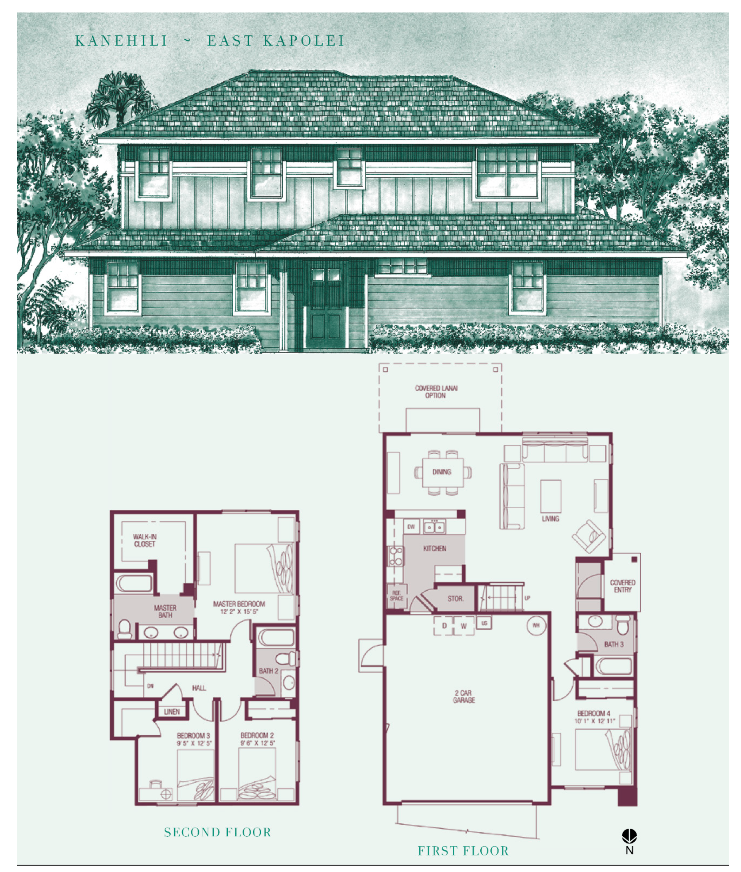
The three to five bedroom detached house typology (Figure 1) featured in this research is in high demand: 62% of buyers seeking housing on Oahu prefer detached houses with three or four bedrooms [18]. Most houses studied are four-bedroom houses, which is similar to Hawaii’s median number of rooms per occupied housing unit of 4.6 in 2019 [18]. This research includes a range of occupants per household, varying from two to eight, which is characteristic of Oahu. While Oahu’s average household size is 2.99, Hawai‘i’s crowding rate has long been among the highest in the nation. An average of 23% of Oahu households in 1992–2019 were doubled up or crowded, which is much more likely in Native Hawaiian households than other households. Doubled up is defined as more than one family per housing unit, and crowded is defined as more than one person per room for 1992–2011 and then two persons per bedroom for 2016–2019, respectively [18].

The houses monitored for this study are located in the DHHL neighborhood of Kanehili in Kapolei, Hawai‘i. Kanehili is a 37-hectare area located at 21°20’19.8” N, 158°03’20.1” W, elevation 23 m. Based on the U.S. climate zone map provided by the International Energy Conservation Code (IECC), the region of study is located in climate zone 1 [19]. There are 390 lots in the neighborhood, with a minimum lot size of 465 m². Over 85% of the houses in the neighborhood are centrally air-conditioned and constructed by one company (builder), including all of the houses presented in this study. The houses studied had three to five bedrooms. The size of the living areas of the houses, which does not include the garage and covered entry, ranged from 141.9 to 155.7 m² and were built between 2009 and 2015 when the Hawai‘i State Energy Code had adopted the IECC 2006.

Table 1. Characteristics of the seven houses included in the study and the dates of monitoring.

House ID#	Total Floor Area (m2)	Living Area (m2)	Bed-rooms	Stories	Year Built	Occupancy	PV	Dates Monitored
1	196.6	148.9	4	2	2015	6 a, c	No	23 June 2017–9 February 2018
2	203.4	155.7	5	2	2010	6 a, d	No	28 June 2017–27 June 2018
3	201.3	153.7	4	2	2010	8 a, c	No f	29 June 2017–28 June 2018
4	201.3	153.7	4	2	2009	2 a, e	Yes	28 June 2017–27 June 2018
5	196.6	148.9	4	2	2009	2 b, d	Yes	15 September 2017–14 September 2018
6	225.4	148.9	4	2	2009	3 a, c	Yes	28 June 2017–27 June 2018
7	189.5	141.9	3	1	2009	3 b, c	Yes	15 September 2017–14 September 2018

^a Occupied often; ^b unoccupied during the day on weekdays; ^c anecdotally uninterested in energy efficiency; ^d anecdotally moderately interested in energy efficiency; ^e anecdotally very interested in energy efficiency; ^f House #3 added photovoltaic (PV) arrays during the year, but it was not metered.

lists the houses, their characteristics, whether they had photovoltaic (PV) arrays, and the monitoring dates. There were two to eight occupants in each house and, anecdotally, their level of interest in energy efficiency varied. Houses #5 and #7 were usually unoccupied during the day on weekdays, whereas all other houses were occupied most of the time.

Houses in the study were constructed of 3.8 cm × 8.9 cm (1.5” × 3.5”) wood studs with R-1.94 m²-K/W (R-11 h-ft²-°F/Btu) batt insulation. There was R-3.34 m²-K/W (R-19 h-ft²-°F/Btu) spray-foam insulation in the conditioned attic at the rafters. The central, ducted air-conditioning capacity was 7 kW (24,000 Btu/h), with a seasonal energy efficiency ratio (SEER) of 16.1, and had a programmable thermostat. The air-conditioning air handling unit with an evaporator coil was located in the conditioned attic and the condensing unit was located outside the house. The houses had ceiling fans or electrical junction boxes for occupants to install ceiling fans. Each house had solar water heating with electric backup and electric appliances, and did not use natural gas or propane. The builder had their houses rated on the Home Energy Rating System (HERS) Index [20] by an independent auditor. The HERS ratings for these houses ranged from 50 to 55, on a scale of one to 100, with a standard new house built in 2006 as the reference at 100, meaning that they are approximately 45–50% more energy efficient than the reference house. The results of this study show that there are still many improvements that can be made.

Each house was monitored for one year between June 2017 and September 2018 (Table 1). A link to the monitored data files can be found in the Supplementary Materials section. The energy monitoring disaggregated the following end-use components: air-conditioning compressor and air handling unit; clothes dryer; stove; kitchen refrigerator; water heater; and PV system if present. For all houses, lighting, non-appliance plug loads, and ventilation fans could not be disaggregated due to shared electrical circuits and are presented together. These demands were estimated by subtracting the monitored end uses from the whole house energy load. Power was monitored continuously and averaged at a one-minute resolution with eGauge^® energy meters (with current transducers), which saves data onboard and does not lose data if temporarily disconnected from the internet. Data acquisition was automated over the internet and inserted into our database using a Python script [21].

The monitored data is considered sufficient for the purposes of this study despite several limitations. House #1 dropped out of the study and was only monitored for 7.5 months (23 June 2017 to 9 February 2018), as noted in Table 1 and Table 4. The energy use for House #1 during non-monitored months was estimated based on its average monthly energy use for non-seasonal loads. The air-conditioning and water heating load for Houses #1, #6, and #9 followed the same seasonal trends. House #1’s missing energy data for these seasonal loads between February and June was estimated by graphing the monthly energy use for Houses #1, #6, and #9 and interpolating the missing values for House #1. House #3 added PV halfway through the study, but it was not monitored. House #7 was missing 21 days of PV data at the start of the monitoring period due to eGauge installation difficulties and the missing data were estimated by copying the first 10 days plus the last 11 days of data for the monitored year. Unexpectedly, the eGauges were sometimes missing minute-level data. Houses #2–#7 were missing no more than 2 h of data over the year for most end uses, except for House #2, which had 24 h of missing refrigerator data. The energy use on days that had missing minutes of data was estimated by multiplying the average power for that house’s end use on that day by 24 h.

The temperature and humidity were monitored with Onset Hobo U12-012 loggers at a fifteen-minute resolution. Four Hobo loggers were placed inside each house: two downstairs and two upstairs (the single-story house only had three indoor loggers). Data from these loggers were manually downloaded during site visits every two to three months. Site visits provided an opportunity for face-to-face meetings with homeowners to answer questions, provide informal education, and receive feedback. The visits also gave student research assistants opportunities to experience the houses they were modeling using energy simulation software. Energy reports giving a monthly breakdown of energy use were mailed to the homeowners. A flyer with energy saving suggestions was distributed at a presentation at a neighborhood association meeting and mailed to the homeowners involved in the study.

2.2. IECC 2015 Energy Model Methods

The team created a whole-building energy model of one of the monitored houses (House #3) using the following software, weather file, and documents. Geometry and construction materials were based on construction drawings, HERS rating reports, and site visit observations. The energy models were created in BEopt^TM v2.8 with EnergyPlus^TM and followed the 2014 Building America Housing Simulation Protocols benchmark specifications [22]. The energy model minimally meets the IECC 2015 standard, which is expected to be adopted by all counties in Hawai‘i in 2020. This model, referred to as “IECC 2015”, was used as the benchmark for the parametric analysis and its inputs are listed in

Table 2. Inputs in BEopt^TM for the International Energy Conservation Code (IECC) 2015 minimum model.

Component	IECC 2015 Minimum Model Inputs
Exterior wall	Gypsum board 12.7 mm (0.5”)
	Wood studs 38 mm × 89 mm (nominal 2” × 4”) spaced 40.6 cm (16”) on center, fiberglass batt R-2.3 m2-K/W (R-13 h-ft2-°F/Btu), oriented strand board, fiber cement finish, medium-dark color 0.04 m2-K/W (R-0.2 h-ft2-°F/Btu) absorptivity 0.75
Unfinished attic	Fiberglass batt at ceiling R-5.3 m2-K/W (R-30 h-ft2-°F/Btu) vented, specific leakage area = 0.0051
Roof	Asphalt shingle, medium color, absorptivity 0.75, No radiant barrier
Ceiling	Gypsum board 12.7 mm (0.5”)
Foundation/floors	Uninsulated concrete slab 10.2 cm (4”), wood floors, no carpet
Window areas	15% of conditioned floor area, 25.0 m2 (278 ft2)
Windows	Double pane, non-metal frame, U = 2.8 W/m2-K (0.5 Btu/h-ft2-°F), SHGC = 0.25, No window overhangs
Interior shading multiplier	Summer = 0.87, Winter = 0.87
Doors/door area	Wood U-Value = 2.84 W/m2-K (0.50 Btu/h-°F-ft2), 3.72 m2 (40 ft2)
Eaves	Roof eave length 0.6 m (2 ft)
Air leakage	5 ACH50
Mechanical ventilation	ASHRAE 62.2 2013 standard, exhaust 41.1 L/s (87.1 cfm), fan power 13.1 W No energy recovery ventilator or heat recovery ventilator
Central AC, cooling set-point, ducts	SEER 14, set-point 23.9°C (75°F), ducts in unconditioned attic, insulation R-0.3 m2-K/W (R-1.7 h-ft2-°F/Btu), leakage 1.9 l/s (4 cfm) per 30.48 m (100 ft) at 25 Pa
Ceiling fan	1.7 Standard efficiency ceiling fans, US national average number of fans
Lighting	75% high efficacy electric lighting
Water heater	Solar: collection area 5.95 m2 (64 ft2), electric resistance backup: energy factor 0.99, cycling derate = 0
Water distribution	R-0.53 m2-K/W (R-3 h-ft2-°F/Btu), trunk branch, copper
Appliances	Standard efficiency refrigerator with a side freezer and ice dispenser, 718 kWh/year, standard electric stove, standard clothes washer, standard electric clothes dryer, no dishwasher
Plug loads	National average energy use

. The IECC 2015 model uses default BEopt^TM assumptions for occupancy in order to represent a typical household.

The simulations used a typical meteorological year (TMY3) weather file for Barber’s Point, which is approximately 3.4 km from the neighborhood. The TMY3 file required cleaning; erroneous temperature values for ten consecutive hours were unreasonably low, at −9.3 °C, and were replaced with temperature values immediately before and after the affected period. This cleaned weather file was used in all simulations.

Some components of existing House #3 are better or worse than the minimum requirements of the standard reference design presented in the performance compliance pathway guidelines of the IECC 2015 Table R405.5.2 [23]. Components of existing House #3 that are different from the IECC 2015 minimum standards include the SEER rating of the AC system of 16 rather than 14, the mechanical ventilation rate from the 2010 ASHRAE 62.2 standard rather than the 2013 version, and zero ceiling fans rather than the national average of 1.7.

The existing solar water heating system uses a standard water heater as the storage tank and electric resistance backup. Oahu does not experience freezing temperatures so potable water is directly pumped to the solar collection panels and no antifreeze is used. Because BEopt^TM does not have this option, NREL (Personal communication, Jeff Maguire, research engineer, NREL, email 12 March 2019) recommended selecting tankless electric with a cycling derate of zero as the electric backup. A link to the BEopt file can be found in the Supplementary Materials section.

2.3. Parametric Energy Simulation and Optimization Methods

After creating the IECC 2015 baseline model, we simulated parametric energy models to compare individual energy efficiency measures in terms of the annual site energy use. Modifications to the building envelope, glazing, HVAC system, lighting, and appliances were tested. By isolating the individual options, it was possible to test their respective impact on the energy use. The parametric models were used to compare the relative percentage energy savings and were not intended to predict the actual energy use.

Prior to the parametric models, a series of local sensitivity analyses where one factor was changed and all other factors were fixed [15] (e.g., testing multiple values for a window solar heat gain coefficient) helped the team understand the range of potential energy savings from individual design components. The sensitivity analyses (not presented in this paper) identified energy efficiency measures’ point of diminishing returns, when, as the performance of a variable was improved, the energy savings were marginal. The sensitivity analyses assisted the research team in selecting the energy efficiency measures presented in the parametric energy analyses.

The team used BEopt’s optimization function to identify the least-cost combinations of energy efficiency measures to achieve either the highest energy savings or the lowest annual energy-related costs. Energy-related costs include utility bills; the cost of adding efficiency measures to the mortgage payment; and the present value of future replacement costs for options with lifetimes of less than the analysis period, typically 30 years [24]. The construction cost multipliers for efficiency measures for Honolulu were entered into BEopt: 1.31 for materials and 1.43 for labor [25]. One monitored house’s electricity costs from early 2017 were used ($9/month fixed cost plus $0.2640/kWh, with an approximate average of $0.2783/kWh).

3. Results and Discussion

3.1. Energy and Thermal Performance of Monitored Houses

The seven monitored houses had the same builder and construction materials and similar HERS ratings, but the site energy use intensity (EUI;

Table 3. Metered annual electricity use and site energy use intensity based on the total floor area and living area.

House ID#	Whole House Electricity Use	Site Energy Use Intensity Based on Total Floor Area		Site Energy Use Intensity Based on Living Area
	(kWh/year)	(kWh/m2/year)	(kBtu/ft2/year)	(kWh/m2/year)	(kBtu/ft2/year)
1	13,636	69.4	22.1	91.6	29.2
2	13,121	64.5	20.4	84.3	26.7
3	14,025	69.7	22.1	91.3	28.9
4	6,187	30.7	9.7	40.3	12.8
5	11,468	58.3	18.5	77.0	24.4
6	12,381	54.9	17.4	83.1	26.4
7	10,455	55.2	17.5	73.7	23.4

) varied by a factor of two due to the variations in the number of occupants, air-conditioning usage, and plug loads. Houses 1, 2, and 3, which have six to eight occupants, have a higher EUI and energy use for the water heater, dryer, and stove (

Table 4. Annual energy use (kWh/year) disaggregated by end use and PV production for the seven metered houses.

	House ID#
End-Use	1 a	2	3	4	5	6	7
AC compressor	5393	5753	5540	1374	5270	5069	3636
AC air handling unit	573	1063	1211	1081	918	1069	706
Water heater	816	548	625	108	387	146	62
Large appliances
Dryer	1393	1274	1128	186	607	856	729
Refrigerator	323	1151	1203	839	714	718	1045
Stove	985	487	571	224	93		212
Plug loads and lights	4153	2845	3747	2375	3479	4523	4065
Whole house	13,636	13,121	14,025	6,187	11,468	12,381	10,455
PV production	0	0	0 b	5422	5262	4066	6851 c
Net use	13,636	13,121	14,025	765	6206	8315	3604

^a House #1’s annual data was estimated based on 7.5 months of metered data; ^b House #3 added PV during the year, but it was not metered; ^c House #7 was missing 21 days of PV data, which was estimated.

) than the houses with two to three occupants. The site EUI was calculated without accounting for PV production for both the living area and total floor area. The living area is defined here as the area inside the house, and the total floor area includes the living area plus the garage and covered entry. The lighting, plug loads, and appliances in the garage (including the washer, clothes dryer, and water heater) for all houses are included in both EUIs for the living area and total floor area. Although unconditioned, the garage often served as a part-time occupied space for a large family, who used refrigerators, computers, TVs, power tools, and other equipment in this space.

Table 4 shows the annual disaggregated metered energy use of the seven houses. Air-conditioning accounted for 40% to 54% of the energy use (mean 47%), similar to the 44% we have seen in military housing on Oahu [7]. House #4 often turned off the AC, which resulted in notable savings: a total annual AC consumption of 2455 kWh vs. a range of 4342 to 6816 kWh for the other six houses. Some homeowners (personal communication with homeowners on various dates and a neighborhood meeting on 23 October 2018) stated that they thought it was better for the AC equipment to run all the time. The manufacturer (personal communication, Rheem customer support, 5600 Old Greenwood Rd, Fort Smith, AR, USA, telephone 19 October 2018) and the local service coordinator (personal communication, Charles Young, Admor, Honolulu, HI, USA, telephone 19 October 2018) said that this was not true.

The solar water heating with electric backup accounted for 1% to 6% of the energy use (mean 3%). Large appliances (the stove, kitchen refrigerator, and dryer) accounted for 12% to 22% of the energy use (mean 18%), although House #6 did not have the stove metered. Lighting and plug loads accounted for 22% to 39% of the energy use (mean 32%). The PV systems on four houses produced 33% to 88% of the houses’ energy consumption (mean 58%).

Air-conditioning is one of the major energy end uses, partly because of the relatively low thermostat set-points. Five of the seven houses had mean indoor temperatures of 23.2 °C (73.8 °F) or below (

Table 5. Mean and standard deviation (SD) of the annual indoor temperature and humidity of the seven monitored houses.

House ID#	Temperature (°C) Mean (SD)		Relative Humidity (%) Mean (SD)
1	22.4	(1.2)	57.5	(2.8)
2	23.2	(1.0)	62.4	(5.6)
3	23.1	(1.1)	63.8	(6.3)
4	26.9	(1.7)	61.0	(5.7)
5	23.0	(2.0)	61.2	(6.0)
6	23.1	(1.2)	58.1	(3.4)
7	25.1	(0.7)	62.4	(6.0)

). The mean interior temperature of all seven houses, 23.8 °C (74.8 °F), is lower than the Building America Simulation Protocol cooling temperature setpoint of 24.4 °C (76 °F) [22] and the 2015 International Energy Conservation Code [23] set-point of 23.9 °C (75 °F). The monitored relative humidity mean was below 64%.

In order to understand how the metered energy use in our study’s Kanehili development compares to other houses in the state, we looked at the NREL study of the Kaupuni development in Waianae, Oahu, HI, to provide a comparative model [14]. Both the Kanehili and Kaupuni studies monitored the energy use in centrally air-conditioned, detached, DHHL houses, with similar air conditioner efficiency ratings of SEER 16.1 and 16 for Kanehili and Kaupuni, respectively, and the same mean indoor temperature of 23.8 °C (74.8 °F). The data in the NREL publication was used to calculate an aggregate EUI for the living area of the combined 19 Kaupuni houses and compared to an aggregate EUI for the living area from this study of the seven houses in the Kanehili sample (

Table 6. Energy use comparison to another Department of Hawaiian Home Lands (DHHL) neighborhood on Oahu studied by the National Renewable Energy Laboratory (NREL) [14].

Neighborhood	Year of Study	Age of Houses (year)	Houses Studied (N)	Living Area (m2)	EUIs Based on Living Area
					(kWh/m2/year)	(kBtu/ft2/year)
Kaupuni, Waianae	2011–2012	0–1	19	121–156	75.7	24.0
Kanehili, Kapolei	2017–2018	7–9 a	7	142–156	77.3	24.5

^a One house was 2–3 years old.

). The Kanehili houses with an EUI of 77.3 kWh/m²/year (24.5 kBtu/ft²/year) were 2% more energy intensive than the Kaupuni houses with an EUI of 75.7 kWh/m²/year (24.0 kBtu/ft²/year). In addition to many other possible factors, the Kanehili houses were eight years older at the time of the study and it is possible that the air-conditioning equipment may have degraded over time, which may account for the slightly higher energy use.

3.2. Parametric Energy Simulation and Optimization Results

The options described in the parametric analysis were included in the optimization unless otherwise noted. Feedback from the builder of the monitored houses was also included.

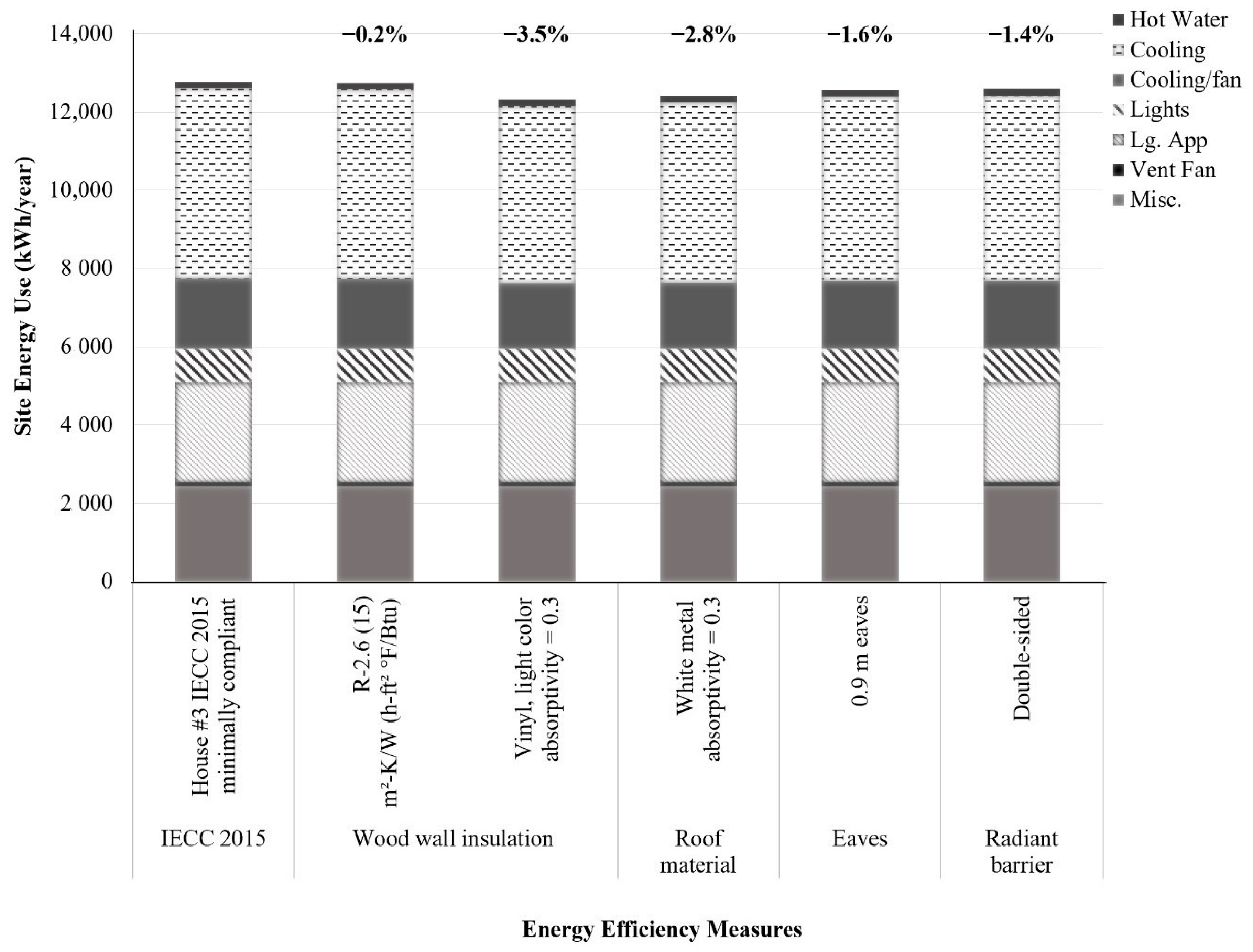
The changes to the building envelope showed modest estimated reductions in annual energy consumption compared to the IECC 2015 case, approximately 0.2% to 3.5%, depending on the measure changed (Figure 2).

• Increasing the nominal R-value of the wall insulation from R-2.3 m²-K/W (R-13 h-ft²-°F/Btu) to R-2.6 m²-K/W (R-15 h-ft²-°F/Btu) showed an energy savings value of 0.2%. During a conversation with the builder, we agreed that the modest energy cost savings do not justify the increased cost of additional insulation.
• Incrementally changing the ceiling insulation from nominal R-5.3 m²-K/W (R-30 h-ft²-°F/Btu) up to R-10.6 m²-K/W (R-60 h-ft²-°F/Btu) showed almost zero energy savings and is not included in the figure or optimization.
• Changing the exterior wall absorptivity from 0.75 (a medium-dark-colored fiber-cement finish) to 0.30 (a light-colored vinyl finish) reduces the annual energy use by 3.5%. During a conversation with the builder, we confirmed that light-colored exterior walls are cheap to implement.
• Changing the roof material from asphalt medium-colored shingles with an absorptivity of 0.75 to a white metal roof with an absorptivity of 0.30 reduces the annual energy by 2.8%. The builder later responded that light-colored shingles are not used because they get soiled by red dirt and algae, and the modest energy savings would not warrant the additional cost of a metal roof.
• Extending the eaves from 0.6 to 0.9 m reduces the annual energy by 1.6%. During a conversation with the builder, an increased overhang depth was determined to be infeasible for their developments due to encroachment on the required setback from the property line.
• Adding a double-sided foil radiant barrier in the roof reduces the annual energy consumption by 1.4%. During a conversation with the builder, it was ascertained that the main barrier to implementation is installing the radiant barrier across multiple roof trusses.

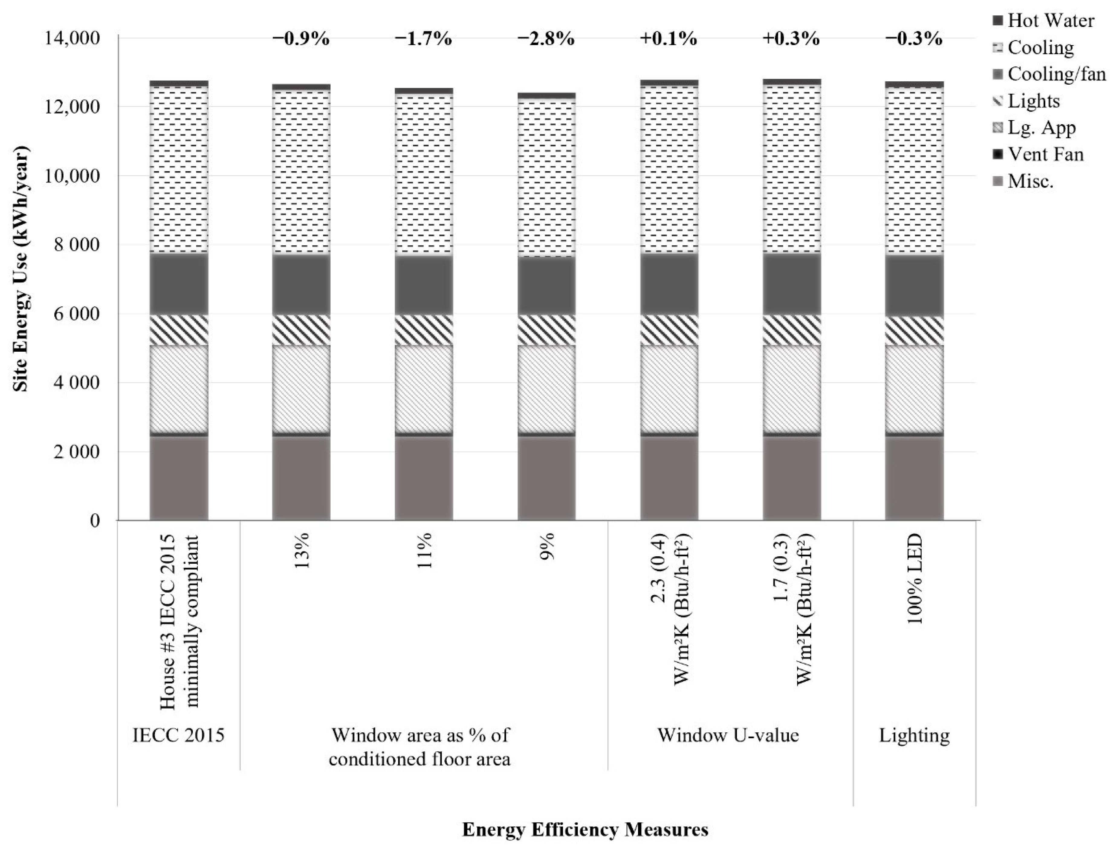
Individual changes to the window performance and lighting efficiency also showed modest changes in the annual energy consumption compared to the IECC 2015 case, approximately −2.8% to + 0.3% (Figure 3).

• Reducing the ratio of the window area to the conditioned floor area from 15% to 9% shows an annual energy savings of 2.8%, due to a reduction in cooling. Developers would not likely reduce the window area due to an undesirable reduction in occupants’ daylight and views. These options were not included in the optimization.
• Changing the window U-values from 2.8 W/m²-K (0.5 Btu/h-ft²-°F) to 2.3 W/m²-K (0.4 Btu/h-ft²-°F) or 1.7 W/m²-K (0.3 Btu/h-ft²-°F) increased the annual energy consumption by 0.1% and 0.3%, respectively. The better-insulated windows trapped heat inside and slightly increased the cooling energy in the evening, especially during the cooler months.
• Adding window overhangs of 0.6 to 0.9 m to all windows decreased the annual energy use by 0.5% and 1.1%, respectively (not shown in the figures; not included in the optimization).
• Upgrading from 75% to 100% high-efficacy electric lighting shows an estimated 0.3% annual energy savings. Although the savings are modest, the measure is recommended because there is little to no increased initial cost. The 75% efficiency was not included in the optimization.

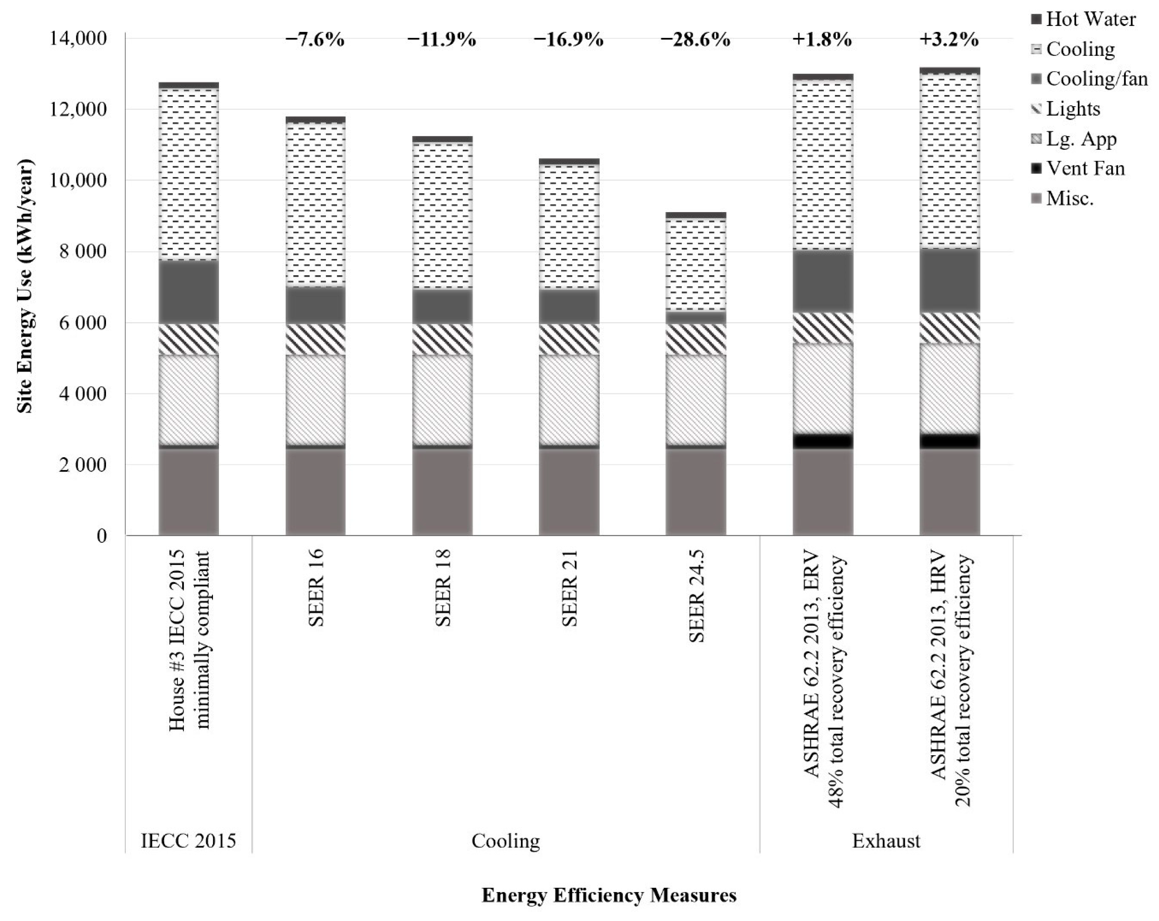
Improvements in the efficiency of the HVAC showed substantial reductions in the annual energy consumption compared to the IECC 2015 case, ranging from 7.6% to 28.6% (Figure 4).

• Increasing the HVAC system efficiency from SEER 14 to SEER 16, SEER 18, SEER 21, and SEER 24.5 results in estimated annual energy savings of 7.6%, 11.9%, 16.9%, and 28.6%, respectively. During a conversation with the builders (in late 2018), we learned that their houses built in 2019–2020 will likely have an SEER 20 rating, representing a notable improvement over the existing or minimally code-compliant cooling systems. The builders appreciated quantitative estimates of energy savings with more efficient air-conditioning systems, which helped them prioritize purchases to meet their goal to reduce energy costs for the homeowner. This energy efficiency measure has a high likelihood of being implemented because the builder controls the selection of the air-conditioning SEER rating (which is a marketable feature), unlike some of the energy-saving measures that rely on occupant behavior.
• The addition of an energy recovery ventilator (ERV; total recovery efficiency of 0.48) or heat recovery ventilator (HRV; total recovery efficiency 0.20 (Personal communication, Kosol Kiatreungwattana, senior engineer, NREL, Golden, CO, e-mail, 30 May 2019 and [26])) increased the annual energy consumption by 1.8% and 3.2%, respectively, mainly due to an increased ventilation fan energy. In other words, the amount of recovered cooling energy was less than the ERV or HRV fan energy. The cooling and cooling/fan energy decreased slightly with the ERV and increased slightly with the HRV. Both were set to use the ASHRAE 62.2 2013 ventilation rate (same as the IECC 2015 benchmark). These were not included in the optimization.

Additional parametric simulations for ceiling fans, the occupancy sensor, and the cooling temperature offset show significant potential energy savings. Increasing the number of fans in the house from 1.7 standard ceiling fans (national average) [22] to five “premium efficiency” fans (meaning that the power needed for each fan is reduced by 50%) increased the annual energy consumption by 3.2% (Figure 5). Five fans were selected in order to have one in each bedroom and one in the main living space. Another option combined the five premium efficiency fans with occupancy sensors so they only turned on when occupied, and increased the cooling set-point at all times from 23.9 °C (75 °F) to 26.1 °C (79 °F). The 26.1 °C (79 °F) cooling set-point is within the comfort zone using the ASHRAE Standard 55–2017 Section 5.3.3 Elevated Air Speed Comfort Zone Method [27]. The Center for the Built Environment’s Thermal Comfort Tool [28], using the Predicted Mean Vote (PMV) method, shows a neutral sensation within the comfort zone for the following inputs: operative temperature of 26.1 °C; air speed of 0.25 m per second (m/s); humidity of 65%; metabolic rate of 1.1 met; and typical summer indoor clothing level of 0.5 clo. A typical living room ceiling fan provides an air speed of 0.254 to 1.016 m/s (50–200 feet per minute) [10]. This reduced the annual energy consumption by 17.6% (Figure 5) and represents the largest energy savings for the occupant-controlled measures tested, but requires diligence from the occupant to turn up the thermostat. Only the option with five fans and the thermostat setback was included in the optimization.

Several parametric energy model simulations were conducted to compare the energy use of standard appliances in the IECC 2015 case to Energy Star or more energy-efficient appliances. After the large appliance parametric simulations were completed, the top energy saving options were placed into one model called “combined energy-efficient appliances” (Figure 5), which showed an 8.1% annual energy savings value compared to the IECC 2015 case and included upgrading the following: the clothes dryer was upgraded from standard electric to premium electric; the clothes washer was upgraded from standard electric to Energy Star compliant; the cooking stove was upgraded from a standard electric stove to an induction stove; and the refrigerator with a side freezer and ice dispenser was changed to an Energy Star compliant refrigerator with a top freezer and no ice dispenser. A dishwasher was not included in the parametric analysis because it was not included in the IECC 2015 benchmark case for this study.

Compared to the DOE Building America list of optimized solutions for cost-effective energy savings for new homes in hot-humid climates [9], this research’s energy models suggest new recommendations: a high reflectance exterior wall and roof; higher (less stringent) recommendations for the window U-value, with a value of 0.5 instead of 0.33; a higher (less stringent) window solar heat gain coefficient of 0.25 due to limited double-pane glazing products [29] being able to meet the DOE value of 0.2; new energy savings estimates with longer overhangs; a higher cooling equipment SEER of 24.5 instead of 18; and no ventilation enthalpy recovery.

The differences between the IECC 2015 minimum baseline model, BEopt optimization’s “least-cost-optimized model” (minimum energy-related costs), and the “energy-optimized model” (maximum energy reduction) are listed in

Table 7. Component differences between the IECC 2015 minimum baseline model, the least-cost-optimized model, and the energy-optimized model.

IECC 2015 Minimum Baseline Model Component	Least-Cost-Optimized Model Components	Energy-Optimized Model Components
HVAC efficiency SEER 14	Variable speed HVAC SEER 24.5	Variable speed HVAC SEER 24.5
No ceiling fans. Cooling set-point 23.9 °C (75°F)	Five premium efficiency fans with occupancy sensorsIncrease the cooling set-point from 23.9 °C (75 °F) to 26.1 °C (79 °F)	Five premium efficiency fans with occupancy sensors Increase the cooling set-point from 23.9 °C (75°F) to 26.1 °C (79 °F)
Appliances: standard efficiency	Appliances: energy efficient, except stove is standard electric	Appliances: energy efficient including induction stove
Exterior finish: medium color with absorptivity of 0.75	Exterior finish vinyl light color with absorptivity of 0.30	Exterior finish vinyl light color with absorptivity of 0.30
Eaves 0.6 m	Same as IECC 2015	Eaves 0.9 m
No radiant barrier	A double-sided foil radiant barrier	A double-sided foil radiant barrier
Roof material: medium color asphalt shingle with absorptivity of 0.75	Same as IECC 2015	White metal roof with absorptivity of 0.30
75% high efficiency lighting	100% LED lighting	100% LED lighting
Window U-value 0.5	Window U-value 0.4	Same as IECC 2015

. The least-cost-optimized model reduced the annual site energy use by 45.5% compared to the IECC 2015 benchmark case, from 12,770 to 6957 kWh/year (Figure 5;

Table 8. Annual energy use (kWh/year) disaggregated by the end use and energy use intensity (kWh/m²/year based on the living area) results for the IECC 2015 minimum model, least-cost-optimized model, and energy-optimized model.

End Use	IECC 2015 Minimum Model		Least-Cost-Optimized Model		Energy-Optimized Model
	Annual Energy (kWh/year)	EUI (kWh/m2/year)	Annual Energy (kWh/year)	EUI (kWh/m2/year)	Annual Energy (kWh/year)	EUI (kWh/m2/year)
AC compressor	4868		1486		1322
AC air handling unit	1779		167		155
Large appliances	2550		1700		1665
Miscellaneous	2430		2500		2500
Lights	865		832		832
Water heating	170		164		167
Ventilation fan	108		108		108
Total energy use	12,770		6957		6749
EUI		83.1		45.3		43.9

). The annual energy-related costs (including additional mortgage and lifecycle costs related to the improved design) for the least-cost-optimized model were reduced by 45.3%, from $3479 to $1904. The energy-optimized model reduced the annual site energy use by approximately 47.1% (Figure 5) to 6749 kWh/y. The annualized energy-related costs for the energy-optimized model were reduced by 39.6% to $2100.

A comparison of the disaggregated annual energy use from the simulations can be seen in Table 8. The greatest savings compared to the IECC model baseline was in the AC energy use (compressor plus air handling unit), with 75.1% and 77.8% reductions for the least-cost-optimized and energy-optimized models, respectively. Large appliances showed 33.3% and 34.7% reductions for the least-cost-optimized and energy-optimized models, respectively.

The energy-optimized model design is depicted in Figure 6. To meet the net-zero energy target, this design would need a grid-tied PV array of only a 4.5 kW capacity (calculations are not presented here) versus an estimated 8.4 kW array for the IECC 2015 minimally compliant design. The 4.5 kW PV array would easily fit on the existing house’s roof. Including other strategies, such as shade trees and using the house in mixed-mode by using natural ventilation when the weather permits, would further reduce the energy needs, but these were not modeled in this study.

3.3. Limitations

The data collection and energy modeling had the following limitations. The BEopt^TM program does not account for electric lighting energy savings that can be gained with daylight. While the existing houses have 18.7% window area to floor area ratios, the IECC 2015 maximum window area is 15% of the floor area, and one parametric simulation had an even smaller window area. The simulations with the reduced window area do not show the potential increase in electric lighting energy. The BEopt^TM program has limited types of insulation materials. The existing houses had spray-foam insulation, but we had to select “fiberglass batt” of the same insulation value, which is less airtight.

4. Conclusions

This study demonstrates, through field measurements and building simulations, that a net-zero energy value is possible for air-conditioned houses in Hawai‘i. It expands the available dataset on detached residential energy use in Hawai‘i, adds new information on disaggregated energy use, and provides insights into air-conditioning operation and interior temperature preferences. Mechanical cooling and plug loads, including appliances, are the major energy end uses with opportunities for incremental improvement.

The houses in the study were built when the energy code was based on IECC 2006. The site EUI, based on the living area, ranged from 40 to 92 kWh/m²/year. They were only 2% more energy intensive compared to another DHHL neighborhood studied by NREL in 2012, which was designed to result in net-zero energy, yet showed potential for improvement beyond even the IECC 2015 energy code.

Air-conditioning accounted for 40% to 54% of the annual site energy use (mean 47%). Six of the seven centrally air-conditioned DHHL houses studied used the air-conditioning all of the time and only House #4 took advantage of natural ventilation at times. House #4 used 59% less energy for air-conditioning compared to the average of the other six houses. This indicates an opportunity to educate occupants on the significant potential energy savings that can be obtained from mixed-mode operation. Occupant education is possible through existing communication methods, such as the homeowner manual currently provided by the builder, homeowners association meetings, or utility bill mailings. The observed continuous use of air-conditioning in a location where natural ventilation can meet indoor comfort 46% of the year (using ASHRAE 55 adaptive comfort standards) warrants further research into occupant motivations and potential for behavioral change.

Mean indoor temperatures for five of the houses ranged from 22.4 to 23.2 °C, which is lower than the cooling set-points referenced in the Build America Protocol (24.4 °C) and the IECC 2015 (23.9 °C). From this, we can infer that many residents prefer temperatures that are cooler than one might expect for residents acclimated to Hawai‘i’s climate. The cooler temperature preference was unexpected and may warrant further research with a larger sample size because current industry guidance [30] states that occupants prefer warm, dry conditions with personal fans. The cooler temperature preference should be a consideration when simulating energy use and sizing a photovoltaic array to meet a net-zero goal in Hawai‘i. The other two houses’ interior mean temperatures were 25.1 and 26.9 °C.

This study provides a replicable process to demonstrate that combined energy efficiency measures and grid-tied rooftop PV can achieve a net-zero energy house design in Hawai‘i. The energy-optimized model reduced the annual site energy consumption by 47.1% compared to a minimally compliant IECC 2015 model. The following measures are listed from highest to lowest energy savings: variable speed SEER 24.5 HVAC; five premium efficiency fans with occupancy sensors and an increased cooling set-point from 23.9 °C (75 °F) to 26.1 °C (79 °F); all energy-efficient appliances; a light-colored exterior finish with an absorptivity of 0.30; extending eaves to 0.9 m; double-sided foil radiant barrier; white metal roof with an absorptivity of 0.30; and 100% LED lighting.

The measures identified in the energy-optimized and cost-optimized models are mostly similar to the prescriptive requirements given in the ambitious U.S. Department of Energy Zero Energy Residential Homes (ZERH) program [31], with the exception of the air-conditioning SEER (18 in ZERH versus 24.5 in this study). This study shows that designers and builders can optimize cost and energy savings with SEER 24.5 air-conditioning systems, which is new information that goes beyond existing aspirational guidance. The modeled energy and cost-optimized measures align with the Hawaii Energy Triennial 2019–2021 Plan’s approach to incentivize energy-efficient HVAC, appliances, consumer electronics, and lighting [32].

This study provides new estimated energy savings with ceiling fans and an increased cooling set-point, but also found that occupants were reluctant to change their behavior, even with in-person education. Other studies have also found that relaxing thermal comfort standards can minimize space cooling energy use in housing in a subtropical climate [33]. The suggestion is not new; a Hawaii energy-efficient home guide [34] has recommended this measure since 2008. Further study is needed to understand why occupants do not pursue the energy savings from this measure and whether occupant education would change their behavior.

The energy-optimized model’s reduction in annual energy use would save approximately 15 metric tons of carbon dioxide equivalents (CO₂e) annually for one house (based on source energy (Oahu CO₂e of 0.7632 kg/kWh [35] and site to source ratio of 3.3 [36])). With Oahu’s approximate electricity cost of US$0.2783/kWh (based on one monitored house’s electricity costs from early 2017), this saves the homeowner annualized energy-related costs of $1379, including the cost of energy efficiency measures added to the mortgage. By extrapolating the energy, emissions, and energy cost savings, this research strives to improve building policies, builders’ practices, and consumer knowledge. From 2012 to 2018, an average of 1061 new detached houses and duplexes, representing 41% of new residential units, were built on Oahu each year [37]. Assuming a similar rate of building over the next five years, if builders implement the information provided by this study, it would reduce CO₂ emissions by almost 79,600 metric tons and residents’ energy cost by almost $7,315,600. Energy efficiency can also reduce the peak electrical demand, which reduces requirements for generating capacity to serve the peak load [38].

Brochures, reports, and presentations were used to communicate to the developer, builder, and homeowners that energy-efficient designs and behaviors can help the State of Hawai‘i to meet its energy goals. Understanding the magnitude of energy savings with various energy efficiency measures is valuable to designers and code officials for informing future designs and energy codes, ultimately helping to meet the State’s goal of 100% renewable energy by 2045.

References

- IPCC. Climate Change 2014: Mitigation of Climate Change, Technical Summary; Cambridge University Press: New York, NY, USA, 2014. [Google Scholar]
- Global Alliance for Buildings and Construction; IEA; UN Environment. 2018 Global Status Report; United Nations Environment Program: Paris, France, 2018; ISBN 978-92-807-3729-5. [Google Scholar]
- State of Hawai‘i. About the Hawai‘i Clean Energy Initiative. Available online: http://www.hawaiicleanenergyinitiative.org/about-the-hawaii-clean-energy-initiative/ (accessed on 10 January 2019).
- Hawai‘i State Energy Office. Securing the Renewable Future. Available online: http://energy.hawaii.gov/renewable-energy (accessed on 10 January 2019).
- U.S. Energy Information Administration. Average Price of Electricity to Ultimate Customers by End-Use Sector. Available online: https://www.eia.gov/electricity/monthly/epm_table_grapher.php?t=epmt_5_6_a (accessed on 10 January 2019).
- U.S. Energy Information Administration. Electricity Data Browser. Available online: http://www.eia.gov/electricity/data/browser/ (accessed on 14 January 2019).
- Peppard, E.; Meder, S.; Maskrey, A.J.; Griffin, J. Energy Audit Results for Forest City Phase I and Phase II. Technical Report for the Hawai‘i Natural Energy Institute. Available online: https://www.hnei.hawaii.edu/sites/www.hnei.hawaii.edu/files/Energy Audit Results for Forest City Building Phase I and Phase II.pdf (accessed on 10 January 2019).
- International Energy Agency. The Future of Cooling; International Energy Agency: Paris, France, 2018. [Google Scholar] [CrossRef]
- DOE Building America. Building America’ s Optimized Solutions for New Homes Hot-Humid Climate. Available online: https://basc.pnnl.gov/sites/default/files/OptimizedSolutions_Hot-Humid_122214.pdf (accessed on 15 April 2020).
- Grondizik, W.T.; Kwok, A.G. Mechanical and Electrical Equipment for Buildings, 12th ed.; John Wiley & Sons: Hoboken, NJ, USA, 2014. [Google Scholar]
- Moore, F. Environmental Control Systems: Heating Cooling Lighting; Mc-Graw-Hill, Inc.: New York, NY, USA, 1993. [Google Scholar]
- Yun, G.Y.; Steemers, K. Behavioural, physical and socio-economic factors in household cooling energy consumption. Appl. Energy 2011, 88, 2191–2200. [Google Scholar] [CrossRef]
- Department of Hawiian Home Lands. About the Department of Hawaiian Home Lands. Available online: http://dhhl.hawaii.gov/about/ (accessed on 18 January 2019).
- Norton, P.; Kiatreungwattana, K.; Kelly, K.J. Evaluation of Model Results and Measured Performance of Net-Zero Energy Homes in Hawai‘i. In Proceedings of the 2013 ASHRAE Annual Conference, Denver, CO, USA, 22–26 June 2013; pp. 1–8. [Google Scholar]
- Wei, T. A review of sensitivity analysis methods in building energy analysis. Renew. Sustain. Energy Rev. 2013, 20, 411–419. [Google Scholar] [CrossRef]
- Heiselberg, P.; Brohus, H.; Hesselholt, A.; Rasmussen, H.; Seinre, E.; Thomas, S. Application of sensitivity analysis in design of sustainable buildings. Renew. Energy 2009, 34, 2030–2036. [Google Scholar] [CrossRef] [Green Version]
- State of Hawai‘i. Hawai‘i Clean Energy Initiative Goals and Objectives. Available online: http://www.hawaiicleanenergyinitiative.org/about-the-hawaii-clean-energy-initiative/goals-and-objectives/ (accessed on 26 June 2020).
- SMS. Hawai‘i Housing Planning Study. 2019. Available online: https://dbedt.hawaii.gov/hhfdc/files/2020/01/FINAL-State_Hawaii-Housing-Planning-Study.pdf (accessed on 26 June 2020).
- U.S. Department of Energy. International Energy Code Council (IECC) Climate Zone Map, Building America Solution Center. Available online: https://basc.pnnl.gov/images/iecc-climate-zone-map (accessed on 20 January 2019).
- The Residential Energy Services Network. Understanding the HERS Index. Available online: https://www.resnet.us/hers-index-score-card (accessed on 20 February 2019).
- ERDL, Scrape-util, GitHub Inc. 2019. Available online: https://github.com/erdl/legacy-scrape-util (accessed on 20 January 2019).
- Wilson, E.; Metzger, C.E.; Horowitz, S.; Hendron, R. 2014 Building America House Simulation Protocols. Available online: https://www.nrel.gov/docs/fy14osti/60988.pdf (accessed on 26 June 2020).
- International Code Council. 2015 International Energy Conservation Code-Third Printing; International Code Council, Inc.: Washington, DC, USA, 2016; ISBN 9781609834869. [Google Scholar]
- Christensen, C.; Anderson, R.; Horowitz, S.; Courtney, A.; Spencer, J. BEopt Software for Building Energy Optimization: Features and Capabilities. Available online: https://www.nrel.gov/docs/fy06osti/39929.pdf (accessed on 26 June 2020).
- Faithful & Gould. Pacific Northwest National Laboratory Residential Energy Efficiency Measures Location Factors 2011. Available online: https://web.archive.org/web/20170125121627/https://bc3.pnnl.gov/sites/default/files/Location_Factors_Report.pdf (accessed on 1 June 2020).
- Minnesota Sustainable Housing Initiative. HRV/ERV Comparison Chart. Available online: http://www.mnshi.umn.edu/kb/scale/hrverv.html (accessed on 9 April 2019).
- ASHRAE. ANSI/ASHRAE Standard 55-2017 Thermal Environmental Conditions for Human Occupancy; ASHRAE: Atlanta, GA, USA, 2017. [Google Scholar]
- Hoyt, T.; Schiavon, S.; Tartarini, F.; Cheung, T.; Steinfeld, K.; Piccioli, A.; Moon, D. CBE Thermal Comfort Tool. Center for the Built Environment, University of California Berkeley. 2019. Available online: http://comfort.cbe.berkeley.edu/ (accessed on 26 June 2020).
- Ander, G.D. Whole Building Design Guide, Windows and Glazing. Available online: https://www.wbdg.org/resources/windows-and-glazing (accessed on 4 September 2019).
- Harriman, L.G.; Lstiburek, J.W. The ASHRAE Guide for Buildings in Hot & Humid Climates, 2nd ed.; ASHRAE: Atlanta, GA, USA, 2009; ISBN 9781933742434. [Google Scholar]
- U.S. Department of Energy. DOE Zero Energy Ready Home National Program Requirements (Rev.07). 2019. Available online: https://www.energy.gov/sites/prod/files/2019/04/f62/DOE ZERH Specs Rev07.pdf (accessed on 26 June 2020).
- Hawai‘i Energy. Triennial Plan Program Years 2019–2021. Available online: https://hawaiienergy.com/files/resources/AnnualPlan_PY19-21.pdf (accessed on 26 June 2020).
- Ren, Z.; Chen, D. Modelling study of the impact of thermal comfort criteria on housing energy use in Australia. Appl. Energy 2018, 210, 152–166. [Google Scholar] [CrossRef]
- Hawaiian Electric Company; Maui Electric Company; Hawai‘i Electric Light Company. Energy Tips & Choices. 2008. Available online: http://www.hawaiicleanenergyinitiative.org/storage/energy_tips_choices_2008.pdf (accessed on 26 June 2020).
- U.S. Environmental Protection Agency. eGRID Summary Tables 2018. Available online: https://www.epa.gov/sites/production/files/2020-01/documents/egrid2018_summary_tables.pdf (accessed on 15 April 2020).
- Hawaiian Electric Industries. 2018 Form 10-K Hawaiian Electric Co Inc Annual Report. Available online: https://sec.report/Document/0000354707-19-000043/ (accessed on 15 April 2020).
- DBEDT. Research and Economic Analysis, State of Hawai‘i Data Book 2018. Available online: http://files.hawaii.gov/dbedt/economic/databook/db2018/section21.pdf (accessed on 26 June 2020).
- State of Hawai‘i Public Utilities Commission. Report to the 2019 Legislature on Hawai‘i’s Energy Efficiency Portfolio Standards. Available online: https://puc.hawaii.gov/wp-content/uploads/2018/12/EEPS-2019-Legislative-Report_FINAL.pdf (accessed on 26 June 2020).
Figure 1.
Elevation (top) and floor plans (bottom) for House #3 and House #4. Modified from copyrighted image from Gentry Kapolei Development, LLC, 2008.
Figure 2.
Simulated annual site energy (kWh/year) consumption for selected parametric building envelope energy efficiency measures vs. the IECC 2015 baseline. Percent changes in annual energy use are labeled.
Figure 3.
Simulated annual site energy (kWh/year) consumption for parametric fenestration and lighting energy efficiency measures vs. the IECC 2015 baseline. Percent changes in annual energy use are labeled.
Figure 4.
Simulated annual site energy (kWh/year) consumption for parametric cooling and mechanical ventilation energy efficiency measures vs. the IECC 2015 baseline. Percent changes in annual energy use are labeled.
Figure 5.
Simulated annual site energy (kWh/year) consumption for ceiling fans, appliances, and the optimized models vs. the IECC 2015 baseline. Percent changes in annual energy use are labeled.
Figure 6.
Energy-optimized model depiction: Items with an asterisk (*) were modified from the IECC 2015 minimum energy model, whilst items with two asterisks (**) were not modeled but are recommended for consideration.