
A Generic Approach to Simulating Temperature Distributions within Commercial Lithium-Ion Battery Systems


1
Technology Development, MAN Energy Solutions SE, Stadtbachstr. 1, 86153 Augsburg, Germany
2
Institute for Sustainable Energy Systems (ISES), Munich University of Applied Sciences, Lothstr. 64, 80335 Munich, Germany
3
Electrochemical Energy Conversion and Storage Systems Group, Institute for Power Electronics and Electrical Drives (ISEA), RWTH Aachen University, Campus-Boulevard 89, 52074 Aachen, Germany
*
Author to whom correspondence should be addressed.
Batteries 2023, 9(10), 522; https://doi.org/10.3390/batteries9100522
Submission received: 11 September 2023
/
Revised: 20 October 2023
/
Accepted: 21 October 2023
/
Published: 23 October 2023
(This article belongs to the Section Battery Modelling, Simulation, Management and Application)
Abstract
:Determining both the average temperature and the underlying temperature distribution within a battery system is crucial for system design, control, and operation. Therefore, thermal battery system models, which allow for the calculation of these distributions, are required. In this work, a generic thermal equivalent circuit model for commercial battery modules with passive cooling is introduced. The model approach can be easily adopted to varying system designs and sizes and is accompanied by a corresponding low-effort characterization process. The validation of the model was performed on both synthetic and measured load profiles from stationary and marine applications. The results show that the model can represent both the average temperature and the occurring temperature spread (maximum to minimum temperature) with deviations below 1 K. In addition to the introduced full-scale model, further simplifying assumptions were tested in order to reduce the computational effort required by the model. By comparing the resulting simplified models with the original full-scale model, it can be shown that both reducing the number of simulated cells and assuming electrical homogeneity between the cells in the module offer a reduction in the computation time within one order of magnitude while still retaining a high model accuracy.
1. Introduction
Large-scale lithium-ion-based battery systems have become an established element of modern energy systems within the last decade. Common applications range from mass markets such as automotive and stationary up to, as of now, niche uses such as electrified marine powertrains [1,2,3,4,5]. Concerning these large-scale battery systems, both investigations on the laboratory scale and the experience obtained from the field have shown that their thermal behavior is crucial over the entire life span. Regarding operational safety, failure cases such as overheating, thermal runaway, and thermal propagation have all proven to be of the highest relevance [6,7,8,9,10,11]. Furthermore, even with below-critical conditions, the temperature still heavily influences important characteristics of Li-ion batteries, such as the impedance behavior or the aging progress [12,13,14,15].
Regarding large-scale battery systems, which comprise multiple cells connected in series and parallel, in addition to the average temperature, the temperature distribution between the individual cells must also be considered. Temperature deviations can be caused by uneven heat generation, as well as by deviating heat capacities or varying heat dissipation from the individual cells to their surroundings [16,17]. Due to the temperature dependency of the battery impedance, temperature gradients cause variations in the current or voltage for cells in parallel or series connections. The influence of temperature differences on the current distribution in parallel connections was investigated by various researchers [18,19,20,21]. Among those, Fill et al. [16] further discussed the occurring positive feedback loop between the electrical and thermal behavior, since current differences intensify existing temperature differences in the system due to the negative temperature coefficient of the battery impedance.
In addition, and as a result of electrical variations, uneven temperature distributions further trigger deviations in the aging progress. Generally, the dependence of aging on the cell temperature is assumed to be of an exponential nature following the Arrhenius law [22]. Zilberman et al. [23] used simulations to investigate the influence of different temperature deltas on the aging rate. The generally negative influence indicated by the results was also verified by several experimental studies, such as those of Chiu et al. [24] and Paul et al. [25]. Within this context, a maximum deviation of 5 K is often given as a rule of thumb in order to avoid severely increased aging [20,26]. The influence of different cooling strategies and cell arrangements is also an ongoing subject of research, as shown by Ji et al. [27] and Cao et al. [26]. Apart from deviating cell temperatures, inhomogeneous temperature distributions within the cells might also influence their behavior, as shown, among others, by Werner et al. [28]. Both inter- and intracell temperature variations relate to the broader topic of cell-to-cell variations (CtCVs) and their influence on the system behavior [17,29,30].
With both the average temperature and the temperature distribution within a battery system being of high relevance for its operation, thermal system modeling has become a major topic in research and development ever since. Thermal battery models are used, among others, for battery design and the optimization of operating regimes. In addition, live applications such as model-predictive control or model-based predictive maintenance are also relevant use cases [31]. The key requirements for suitable models for such applications are accuracy and spatial–temporal resolution, as well as computational demand and easy parameterization for different system structures.
The foundation of a thermal battery system model is the battery cell model. Cell models can represent different degrees of cell internal inhomogeneity. The most common are so-called 0D lumped parameter models as used, among others, by Shadman Rad et al. [32], which assume equal temperature and electrothermal characteristics within the entire battery cell. Models including 1D models [33,34], 2D models [35], or 3D models [36,37] increase the geometrical complexity accordingly and are used, among others, during the geometrical dimensioning of a cell or the investigations of cell internal defects such as nail penetration. Scaling these cell models to the system level requires the representation of the thermal interaction with other cells, passive components such as the system housing, and the environment. This can be achieved by using highly resolved computational fluid dynamics (CFDs) models [26,38,39]. These models allow for a precise representation of the system’s geometry and the calculation of complex phenomena such as heat convection. However, in return, they require extensive knowledge about the system’s geometrical structure and used materials, thus rendering the parameterization challenging. Also, the resulting models are usually very demanding during computation, thus hindering an effective usage in live model applications.
Another approach is given by so-called thermal equivalent circuit models (T-ECM), which represent the thermal interactions in the system through electrical components such as resistors and capacitors. Thermal equivalent circuit models can incorporate different degrees of spatial resolution, ranging from complex 3D models as given, among others, by Kleiner et al. [29] up to highly simplified models incorporating 0D cell models as given, among others, by Gan et al. [40] and Murashko et al. [41]. A comparative study on the influence of the model complexity on accuracy and computational effort is given by Lechermann et al. The authors in [42] tested various levels of order reduction for a 3D thermal module model, as well as implemented artificial neural networks as surrogate models [42]. In general, thermal equivalent circuit models enable a considerably faster computation in exchange for often limited accuracy and resolution. However, they usually still require an extensive parameterization and often do not allow for live computation when applied to large-scale systems consisting of thousands of individual battery cells.
Following this conflict of interests, the present work intends to contribute the following aspects to the state of the art of thermal battery system modeling:
- A thermal battery system model for a commercial Li-ion battery module with a focus on computational simplicity and easy adaptation to other module geometries.
- A corresponding parameterization approach, which allows for the rapid determination of all of the required parameters without causing irreversible damage to the module.
- An analysis of further simplifying assumptions, which reduces the model’s resolution and accuracy in exchange for faster computation.
The resulting modeling approach intends to extend the electrical model proposed in [43] through a thermal perspective providing a holistic tool chain for the electro thermal modeling of large-scale battery systems.
In order to enable a meaningful evaluation of the proposed thermal battery model, reference indications for the model accuracy and computational cost are necessary. For this purpose, quantitative excerpts taken from existing publications are presented in the following. It must be mentioned, however, that the complexity of the system under investigation strongly influenced the achievable model accuracy, hence limiting the comparability with different modeling approaches. Regarding the computational performance, deviations of the model depth and the performance of the executing system and solver algorithm further hindered comparisons between different modeling approaches. Therefore, a quantitative comparison can always only serve as an indication for the evaluation of a model.
Regarding single cell models, the published results often exhibit maximum model errors of around 1 K, e.g., 1.5 K in [34] and 1.35 K in [35]. At the module or pack level, errors of up to 3.3 K [38], or 5 % of the measured temperature [40], can be found. Higher accuracies are, among others, given by Lechermann et al. [42] and Kleiner et al. [29] with maximum errors below 1 K and 0.5 K, respectively. In terms of the computational effort, the published results vary to an even higher degree. The highly spatially resolved model proposed by Trady et al. [36] requires beyond 1000 s per hour of simulated profile. On the other end of the spectrum, Lechermann et al. [42] describe various model designs achieving below 1 s per hour profile time, although these do not include initialization and postprocessing [42].
2. Experimental Setup
2.1. System under Investigation and Experimental Setup
During the investigations, a lithium-ion battery module manufactured by LG Energy Solution was used. The module comprises 28 64 Ah NMC pouch cells with a maximum load rating of in a 14s2p configuration. Within the module, the cells are grouped into two 1D cell stacks with 14 cells each, which are separated by an isolation pad (see Figure 1). The applied cell numbering indicates each cell’s serial position along rising electrical potentials. The individual cells are electrically interconnected by copper connection plates and geometrically separated by aluminium spacers. The interconnections between the two submodules, as well as between the sub-modules and the power terminals, are achieved via solid copper busbars. The entire module is housed in an aluminium casing with additional steel elements at supporting positions.
During the measurements, the module was connected to a Scienlab SL/80/100/8BT6C battery tester with an additional SL/U/MCM16C unit for the individual measurement of all 14 cell voltages. In total, current and voltage were measured with an accuracy of and , respectively. All measurements were conducted in an ATT DM340T climate chamber. In order to measure the temperature distribution inside the module, 14 type K thermocouples were inserted into every second aluminium spacer (see Figure 1). The temperatures recorded by these sensors are, in the following, referred to as cell temperatures . Additional thermocouples were placed onto the housing () and the positive and negative terminal (, ), as well as inside the climate chamber in order to record the ambient temperature (). The sensors were integrated via two PEAK Systems MU-Thermocouple1 CAN modules. In order to quantify the resulting accuracy, the entire sensor chain was compared to a Lufft XP100 reference sensor. For this purpose, five thermocouples and the reference sensor were inserted into a distilled waterbath and tempered to 10, 20, 30, and 40 . The measurements resulted in a mean deviation of −1.12 K compared to the reference sensor with a maximum deviation of 0.37 K between the individual sensors. The determined mean error was not compensated in the following but was taken into account during the model validation.
2.2. Analytical Investigations
Some of the characteristics that are relevant to the following model parameterization can be obtained without conducting actual electrothermal test procedures. In the first step, the elements of the module housing were disassembled and weighed in order to calculate the corresponding heat capacities derived from the literature values. By disassembling the rear cover of the module, one of the aluminium spacers was also accessed and weighed. All weighing was conducted with a Kern PNS 3000-2 laboratory scale. The resulting masses m and heat capacities are given in Table 1. A potential nondestructive approximation to this process would be to calculate the housing mass from the total module weight and the cell masses given by the data sheet.
In order to determine the thermal resistances of the copper busbars interconnecting the submodules and the module terminals, the Wiedemann–Franz law was applied. The Wiedemann–Franz law (Equation (1)) describes the relation between the electrical conductivity and thermal conductivity in metals as proportional to the temperature T with the constant [44].
Using this relationship, the determination of the thermal resistance for complicated geometries can be substituted by the relatively simple measurement of the electrical resistance. Busbar 1 connects the positive pole and the first submodule, while busbar 2 connects the negative pole to the second submodule. Busbar 3 interconnects the two submodules. All electrical resistances were measured with a Gossen Metrawatt Metra Hit H+E CAR. The resulting thermal resistances for a reference temperature of 25 are given in Table 2. In addition to the busbars, the thermal resistance of the isolation pad between the two submodules was analytically determined from the thickness of the pad and the material properties of expanded polystyrol (EPS).
2.3. Steady-State and Cooling Curve Measurements
While some characteristics can be obtained by direct measurement or analytical calculation, most of the thermal properties of the battery module must be obtained via specific experiments if the process is meant to be nondestructive. Consequently, various steady-state–cooling curve (SSCC) experiments have been conducted for this study [45]. During the steady-state tests, the module was continuously stressed by alternating 5 s current pulses. The corresponding losses in the form of irreversible heat generation, also called Joules heat generation , heated the module until a steady state was reached. During these experiments, the steady state was defined by a temperature change below . The reversible heat due to entropy changes can be neglected, since it changes sign with the current and, therefore, does not, on average, account for additional heating. In the steady state, the heat dissipated to the environment equals the heat generated from the pulses. Figure 2 shows the module current and the corresponding average cell voltage for a 20 h heating period with a load of 2C/3. All experiments were conducted at a state of charge (SoC) of 50%.
Figure 3a depicts the resulting temperatures of the cells and the housing at an ambient temperature set point of 20 . The experiment was repeated at four different loads between C/2 and 1C (see Figure 3b).
Since the heat generation can be attributed to the electrical losses, its value can be calculated from the module current , the average overvoltage , and the number of cell pairs in series :
In theory, can be determined by subtracting the initial average open circuit voltage () measured before the experiment from the measured voltage during the heating period. However, this only holds as long as the battery remains in the electrical steady state i.e., no changes in the SoC occur. As shown in Figure 2, this assumption was not valid for the conducted experiments. The visible drift in the measured voltage indicates a SoC change, which is most likely due to imprecise current measurement and control. Investigating the OCV before and after the heating phase allows for the determination of the occurring SoC drift, which amounts to just below 1% for the 2/3C profile. In order to account for this effect, the OCV curve (dashed yellow line) was calculated as the linear interpolation between the initial OCV and the OCV after the heating period.
By measuring the temperature difference between the cells, the housing, and the environment, the equivalent thermal resistance can be calculated according to Equation (4) using the mean heat generation in the steady state. Table 3 lists the measured temperature deltas between the cells and the environment (C2A), between the cells and the housing (C2H), and between the housing and the environment (H2A), as well as the calculated heat generations and resulting thermal resistances.
Following the 20 h heating phase, the pulsing terminated and the module cooled down to ambient temperature (see Figure 3). During cooling, heat from the cell stack was dissipated via the housing to the environment. Equation (5) approximates the temperature trajectory using the starting temperature and the thermal time constant .
By fitting this equation to the measured curves, the thermal time constant can be determined. When applying this method, the entire cell stack is considered as a homogeneous heat capacity with equal temperature. Inhomogeneous temperature distributions may result in distortions of the pure exponential trajectory. Since the remaining mean absolute error during fitting was found to be below 0.02 K, this assumption was considered uncritical. With the thermal time constant being the product of the cell stack heat capacity and the thermal resistance , the corresponding heat capacity can be determined. The results are given in Table 3.
2.4. Entropy Variation Measurements
During the operation of a Li-ion-based battery system, the entropy variation as a function of the SoC must also be considered as a relevant characteristic due to its corresponding heat generation , which is given by Equation (6) using Faraday’s constant F:
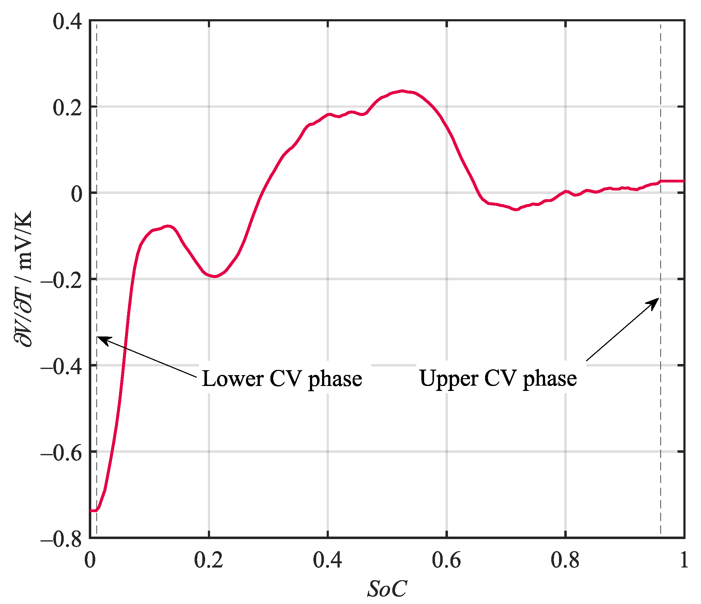
Various potentiometric and calorimetric methods for the determination of the entropy heat coefficient (EHC) i.e., , have been proposed by researchers. The method applied in this work is a dynamic calorimetric approach introduced by Damay et al. [46]. It is able to determine a high-resolution entropy curve in a comparably short time by recording the temperature development during a full charge and discharge cycle under a constant current–constant voltage (CC-CV) regime. By calculating the temperature gradient from the recorded temperature curves and multiplying it by the stack heat capacity , the heat balance can be derived. Using the thermal resistance , the dissipated heat can be calculated. The remaining total heat generation can be understood as the sum of the irreversible Joules heat and the entropy heat . While the entropy heat changes sign with the current, the Joules heat is always positive, i.e., heating. Therefore, the difference between the two total heat generations equals the sum of the entropy heat generations in charging and discharging direction. This derivation is accurate assuming a negligible current dependency of the internal resistance. The resulting entropy curve obtained during a C/2 CC-CV cycle is given in Figure 4. The dashed lines mark the regions during which the constant voltage regime was active. These regions cannot be used to determine the EHC with the given method, since the current was no longer equal in charging and discharging direction. The curve was, therefore, held on the last valid point during these sequences.
3. Modeling
3.1. Electrical System Modeling
As shown in Section 2, the calculation of the heat generation in a battery cell requires information from the electrical domain, such as the SoC and the Joules losses. For this reason, a thermal battery model is usually directly coupled with a corresponding electrical model that is able to calculate these values. The thermal model used in this work was coupled with the electrical battery system model described in [43]. The underlying electrical cell model consists of an SoC calculation via Coulomb counting and an ECM with a serial resistor and two RC elements. The open-circuit voltage includes a linear zeroth-order hysteresis model, while the overvoltage was calculated in dependence of the SoC and cell temperature.
In order to scale the electrical cell model to the system level, the cell model was instantiated separately for every physical cell in the system and interconnected according to the actual cell topology (see Figure 5). Every instance of the cell model was parameterized with its own resistance and capacity deviation, and , respectively, as well as its individual initial state of charge , thereby allowing for the calculation of the voltage distribution within the system. The influence of the cell connector resistances is not considered within the electrical model. The total connection resistance can be determined from the difference between the module voltage measured at the terminals and the sum of the cell voltages under load. Calculating the connection resistance from the entropy variation test data resulted in total resistance of 0.37 m, which can be neglected compared to the sum of the cell resistances.
The electrical system model is fully implemented in the object-oriented Modelica modeling language using its open-source distribution OpenModelica. The model parameterization used in this work was taken from [43]. It was experimentally obtained for the same battery module as was used for this work.
3.2. Thermal System Modeling
In the thermal domain, each cell is modeled as a 0D heat capacity by approximating a uniform temperature within the entire cell. This assumption is regularly considered acceptable due to the high internal thermal conductivity compared to the heat transfer to the environment [47]. The internal heat generation of each cell is calculated from the sum of the power losses at the resistive elements in dependence of the current and the entropy heat according to Equation (7). Further heat sources such as the heat of mixing are usually considered negligible and are therefore not included [34]. For a more detailed investigation of the individual contributions of different heat generation terms to the total heat generation, the reader is referred to [48,49].
Since every cell model was individually parameterized with , , and , the Joules losses were also calculated cell specifically. The entropy curve used in the cell-specific calculation of the entropy heat was assumed to be equal for each cell.
In order to aggregate the single cell model instances into a thermal system model, they were connected to each other, as well as to the housing and the environment, via various thermal resistors. The resulting thermal equivalent circuit model for the battery module is shown in Figure 6. The module housing was approximated as a uniform heat capacity . This assumption is expected to be valid due to the high thermal conductivity of the metallic housing and the comparably small temperature deviations between the single cells. Each cell was connected to the housing via a thermal resistor , which can be individually parameterized for every instance. The cell-to-housing resistors represent both the heat transfer via the adjacent surfaces and the convective transmissions of the cells to the housing. The housing heat capacity was further connected to the ambient potential via a thermal resistor , whose value was set in dependence to the housing temperature. This dependency represents the variable convective flow conditions, among others, induced by the speed of the main fan in the climate chamber, which increases at higher heat losses of the module to the environment.
The thermal interconnection of the cells via the aluminium spacers was modeled by an additional heat capacity and two corresponding thermal resistances . The resistors represent both the direct conduction via the adjacent surfaces and the heat conduction via the copper cell connectors. The combination of the cell and spacer with their corresponding thermal resistances forms a repeatable unit within the model. In addition to the spacers, the two submodules were separated by a thermal resistor representing the isolation pad in the center of the module. As introduced in Section 2.1, the cells in the front, rear, and center were also interfaced by three copper busbars, which were each modeled via a thermal resistor . The temperatures measured at the terminal poles of the module were introduced as the temperature potentials and and form the model boundary. Since these temperatures are usually not measured during the operation of commercial battery modules, the thermal interconnection between different modules via the terminal poles must also be considered when investigating installations on the rack, pack, or system level.
The introduced thermal equivalent circuit model can be easily adapted for different 2D geometries consisting of cuboid cells, such as pouch or prismatic cell types. Cylindrical cells, which can be arranged in different geometries, require a further adaption of the model. Also, active air or liquid cooling systems are not represented by the given model approach as of now. In order to include such systems, an additional set of thermal resistances would need to be included, which would connect the cells to the thermal potential of the cooling stream. The relevance and implications of this expansion are further discussed in Section 6.
The battery-system model described in Section 3.1 and Section 3.2, as well as the corresponding parameterization introduced in the following section, are publicly available for use by other researchers. For access details, refer to the data availability statement.
3.3. Parameter Generation
In order to determine the parameters of the thermal battery system model, the experiments described in Section 2.2, Section 2.3 and Section 2.4 were used. The heat capacities and , as well as the resistances and , were directly obtained through the measurements described in Section 2.2. The cell heat capacity was determined by subtracting the heat capacity of all of the spacers in the module from the stack heat capacity (see Table 3) and dividing the result by the number of cells in the stack. The resulting heat capacity of the single cell was calculated to be 1587 J/K. At a data-sheet cell weight of 1163 g, this results in a specific heat capacity of 1364 J/gK. When compared to the literature values as aggregated by Steinhardt et al. [50], this value falls slightly above usual values, which is most likely due to the consideration of the cell connectors within the cell heat capacity. For the thermal resistance , the results of the SSCC experiments given in Table 3 were used as a temperature-dependent lookup table.
While the majority of the parameters can be determined directly from the SSCC experiments, the cell-specific cell-to-housing resistances and the cell-to-spacer resistances require further analysis, since the distribution of the total heat flow to the individual surfaces cannot be determined without direct measurement. Therefore, numerical optimization was chosen for the determination of the remaining parameters. For this purpose, the introduced thermal equivalent circuit model and the measured temperatures taken from the steady-state experiments (see Figure 3) were used. Since the steady state is concerned, all of the heat capacities within the equivalent circuit can be neglected. Furthermore, the above-introduced thermal resistances and the heat generation were given as known parameters. Using the resulting model, a set of simulated temperatures can be calculated and compared to their measured counterparts. By minimizing the resulting sum of squared errors (SSEs), the optimal parameter set can be determined:
In theory, the given optimization allows for the determination of an individual parameter for each cell k in the module. However, in order to achieve stable fits, the number of degrees of freedom must be significantly reduced. Therefore, the value for was assumed to be equal for all of the cells apart from the cells directly at the front and rear of the module. This corresponds to the equal perimeter housing surface adjacent to each cell. By employing this simplification, four parameters remained as the degrees of freedom during the optimization. The results of the optimization with the differential evolution algorithm [51] are given in Table 4 for all of the four SSCC experiments, as well as the average values, which were further used for the model parameterization. Even though they were clearly within distinct ranges, the results still show a visible deviation present in the four SSCC experiments. This relates to the simplifications made during the model design, especially the likely temperature dependency of the thermal resistances used to model the heat transfer between the cells in the housing and the heat transfer via the busbars.
4. Validation
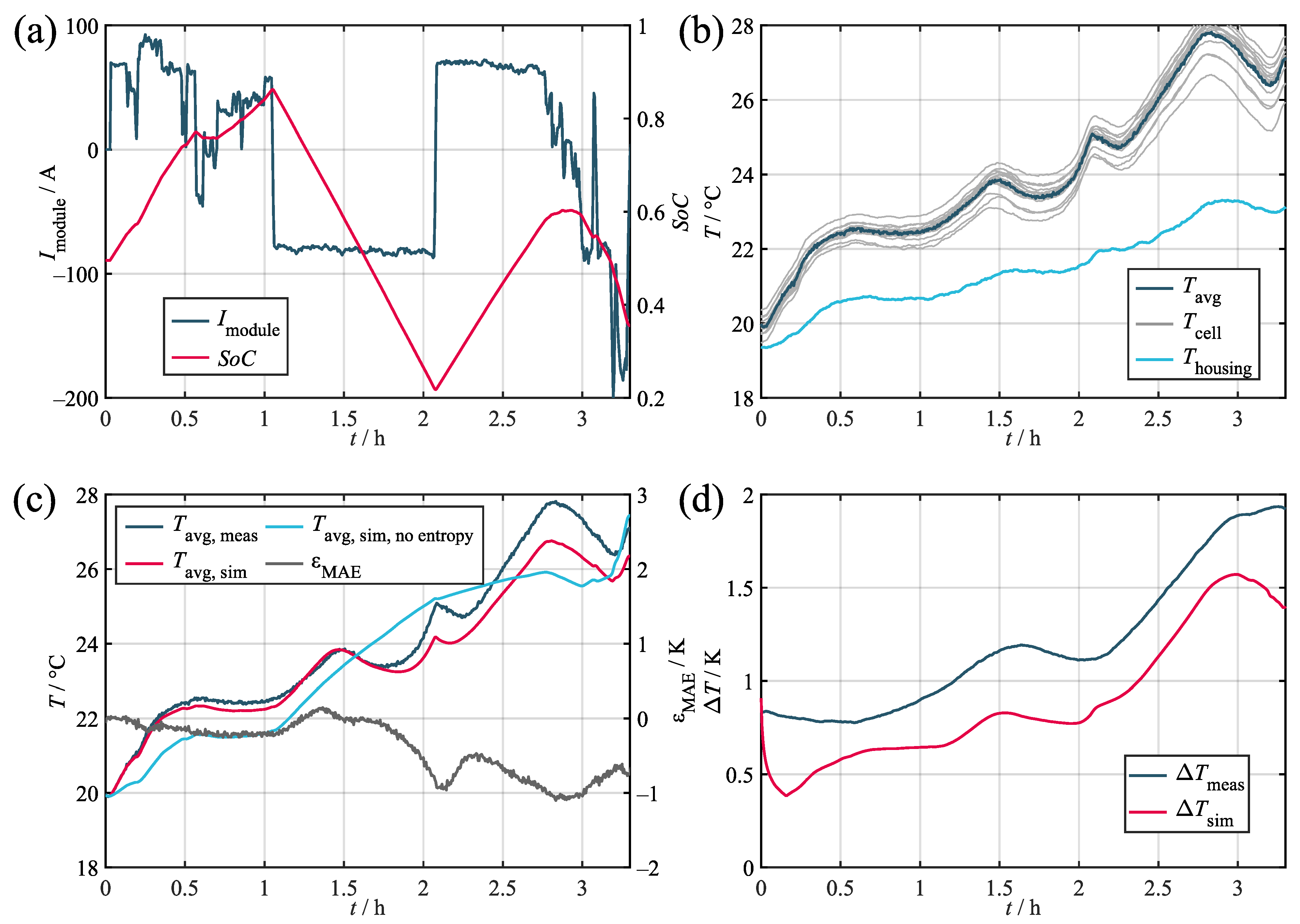
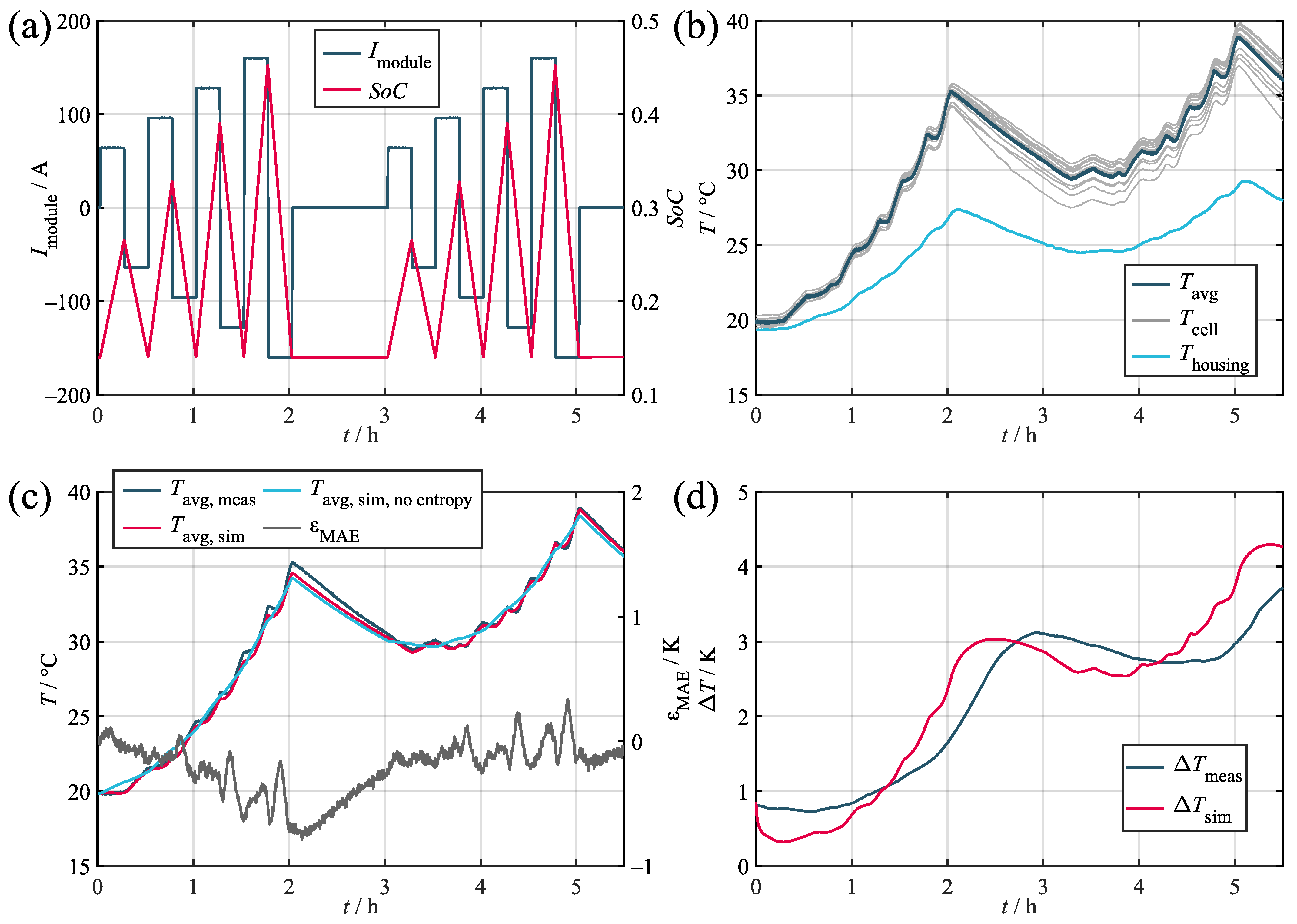
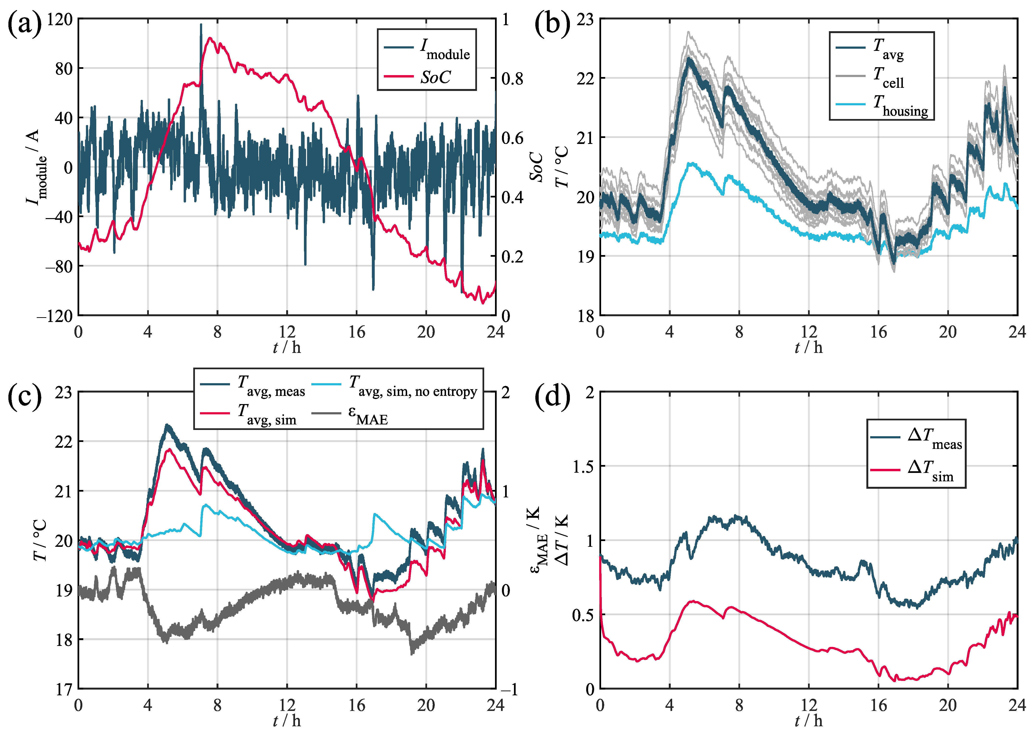
In order to quantify its accuracy, the model was tested against three different load profiles taken from different applications. Their corresponding key parameters are given in Table 5. The results obtained during the validation are given in Table 6 and shown in Figure 7, Figure A1, and Figure A2. Within the figures, the subplots labeled as (a) depics the load profile and the corresponding SoC trajectory. The subplots labeled as (b) show the corresponding measured temperatures of the cell stack, the housing, and the environment. All of the validation measurements were preceded by a full CC-CV charging procedure and consequent discharge to the initial SoC. Prior to commencing the measurements, both thermal and electrical relaxation were achieved via a waiting time of 24 h. The comparison of the average measured and simulated temperatures and the resulting error values are given in the subplots labeled as (c). The average was derived from the temperature of the 14 thermocouples both in the measurement and simulation, where the temperatures of the spacer heat capacities were taken as a suitable substitute. In order to further quantify the representation of the temperature distribution, the temperature spread was used. The subplots labeled as (d) show the occurring spread during both the measurement and simulation. The temperature spread was chosen as a quality criterion, because it is a good indicator for the potential consequences of the temperature deviation in the module and allows for simple interpretation. The validation data recorded during the testing of the synthetic profile is publicly available for use by other researchers. For access details, refer to the data availability statement.
Regarding the average temperature, the validation confirms that the model can represent the measurement accurately with maximum absolute errors of ca. 1 K in the worst case and a 0.28 K mean absolute deviation across all of the profiles. Upon comparing the three profiles, the model proved to be more precise in relative terms for higher loads. This relates to the increasing impact of the entropy heat component at low loads compared to the Joules heat component. Since the entropy heat coefficient is usually only within the range of hundreds of microvolts per Kelvin and, therefore, requires highly accurate measurement devices and conditions, its determination is susceptible to inaccuracies. As can be seen, the stationary and marine profiles in particular showed significant decreases in accuracy when neglecting the entropy heat due to the comparably low loads applied and the quadratic nature of the Joules heat component.
Regarding the temperature spread, a maximum deviation of about 2 K can be observed for the marine profile with increasing spreads at higher average temperatures. During simulation, it can be seen that, while matching the overall course, the simulation fell consistently below the measured curve. This offset error relates to the sensor accuracies described in Section 2.1, with the five thermocouples tested showing an internal deviation of 0.37 K. This was not replicated by the model, which caused the initial temperature spread to subside fairly quickly before the distribution originating from the actual load developed. The same behavior can also be observed for the stationary profile (Figure A2), thereby indicating a steady offset error of ca. 0.5 K. In this context, the observed maximum sensor deviation of 0.37 K is also expected to increase when testing larger samples of sensors.
While the marine and the stationary profiles both showed a trajectory comparable to the measurement with a distinct offset error, the synthetic profile (Figure A1) requires further interpretation. Although the initial drop in the temperature spread associated with the sensor deviation is clearly visible, the simulated curve surpassed the measured reference during both of the load phases. This effect most likely relates to the heat transfer via the terminal busbars. During the test procedure, the terminals surpassed temperatures of 50 . Since, in the model, the terminals are directly coupled to most of the inner and outer cells via two thermal resistors, even incurring small inaccuracies while determining the value of the said resistors can lead to comparably large temperature increases. This effect is especially visible for the synthetic profile, since it incorporated the highest average load of the three profiles.
5. Model Simplification
The model as hitherto presented requires about 660 s of computation time for running the synthetic 5.5 h load profile in a secondwise resolution on a performant desktop PC. While 120 s/h can be considered acceptable for running few simulations on a single battery module, a potential live simulation of a large-scale system consisting of hundreds of modules would require tremendous computational power and would, therefore, cause significant costs for the operator. In order to enable such applications, a simplification approach for the presented model is introduced in the following. The objective is the reduction of the computational effort while retaining the model quality of the original full-scale model.
5.1. Derivation
In order to derive a simplified model version, the original cell-discrete model was converted into a continuous model. As shown in Figure 8, the battery module was considered to consist of two homogeneous thermal masses separated by the isolation pad. Both of the thermal masses hold a temperature distribution in dependence of the longitudinal position x and independent of the lateral position. Within the homogeneous thermal mass, a vertical slice of length comprises the heat capacity and the position- and time-dependent heat generation . The heat capacity includes the heat capacities of the cells, as well as the spacers, and is considered to be equally distributed along the module length.
The individual increments were further interconnected by the thermal resistance and connected to the housing via the thermal resistance . In assuming a homogeneous thermal mass, is independent of x. In contrast, the cell-to-housing resistance must be considered as variable over x in order to represent the increased heat transfer at the front, i.e., the rear as well, of the module. The given description can also be formulated as Equation (9) according to Fourier’s law of thermal conduction:
To solve Equation (9), the model must be discretized along the x axis, with the number of increments determining the resulting computational effort and accuracy of the model. Simulating the model in 28 increments corresponds to the full-scale model presented in Section 3 with merged spacer and cell heat capacities. In the following, the effects of reducing the number of discrete increments on the achievable computation time and model accuracy were tested. During this process, the additional elements apart from the cell stack (housing, isopad, and copper busbars) were implemented according to the full-scale model.
5.2. Verification
For the verification of the derived simplified model, its performance was compared to the reference model results given in Section 4. Figure 9 shows the increase in the mean absolute error for the average temperature (a) and the temperature spread (b) over the achievable simulation time normalized to a one hour profile time. Data point 1 shows the reference model with 28 cells, while points 2–6 show the the results for the model simplification discretized in 28, 20, 14, 8, and 4 increments. The results indicate the expected conflict of objectives between simulation duration and additional error, with the error increasing significantly for low numbers of increments. It can also be seen that the temperature spread was much more susceptible to the reduction in increments, which almost doubled the original mean absolute error of the full-scale model for the four-increment simplification. In investigating the underlying sensitivity, the required computation time can be plotted over the number of increments. The resulting curve shows a strong quadratic relationship, thus suggesting the complexity of the problem in asymptotic notation.
In addition to reducing the number of increments, the computational speed can also be increased by changing the nature of the electrothermal model coupling. In the full-scale model, every thermal cell model is coupled with an individual electrical cell model, thus enabling a cell-specific calculation of and the consideration of a cell-specific within the electrical model. Simplifying this approach by only calculating an average electrical behavior using the average temperature as an input and an average heat generation as the output allows for a further reduction in the computation time. Figure 9 shows the results of this electrically homogeneous approach. It can be seen that, for the same number of increments, the computation time was severely reduced, while the error increase was comparably low for large numbers of increments. This corresponds to the comparably small influence of the electrical behavior deviations on the temperature distribution. However, it can still be seen that, even for the reference model, assuming electrical homogeneity induced a distinct model error. Further reducing the number of increments did not initially affect the error significantly. This is due to the fact that the error resulting from the electrical homogeneity and the error resulting from the reduction in increments annul each other. Going further towards eight or four increments, the effect of the reduction in increments surpassed this effect and caused a significant increase in the model error.
While these results might suggest that assuming electrical homogeneity is a promising tool to achieve fast computation, it must be noted that this approach does not allow for an investigation of the electrical effects of large temperature spreads in the model. Also, the induced error might be significantly increased as soon as systems with large electrical CtCVs, e.g., aged systems, are simulated.
6. Discussion
The battery model introduced in this study offers an approach to thermal system modeling, which is easily adaptable to various module structures and designs. The corresponding parameterization procedure allows for the determination of all of the relevant parameters using comparably simple electrothermal measurements conducted with standard battery testing equipment. Also, the parameterization process can be conducted without disassembling the cell stack, i.e., opening the cell connectors, which would render the module unusable for further testing. However, it is still necessary for both the parameterization and validation of the model to measure the temperature distribution within the module, which was achieved by inserting additional temperature sensors into the module. To what extent reducing the number of sensors used during the experiments affects the quality of the resulting model parameterization is to be tested in further investigations. Also, promising and completely noninvasive methods such as impedance-based temperature determination, as introduced, among others, in [53,54], must be assessed in order to further simplify the parameterization process.
During validation, the general model quality was proven through the example of three load profiles with different load characteristics. With maximum absolute errors significantly below 1 K in almost all of the scenarios, the resulting model accuracy falls well within the range of the existing literature models presented in Section 1. The results also show that neglecting entropy-based heat generation causes significant model errors, especially for low-current load profiles. This contradicts the repeatedly made assumption that entropy effects can be neglected without inducing major model errors. Regarding the temperature spread as the key quantity for assessing the system behavior, the model was generally able to follow the measured trajectory. However, the offset induced by the sensor deviation was identified as a relevant error source, which must be taken into account when applying the model. Furthermore, the representation of the busbars connecting the cells to the module terminal is also likely to have a large influence on the simulated temperature spread.
In its presented form, the model requires around 120 s per hour of profile time to compute. In order to further reduce the computational effort, a continuous model description was derived and discretized using varying numbers of increments. The comparison of the simplified model to the reference shows that the achievable reduction in computation time and the additional induced error are in conflict. Nevertheless, significant reductions in computation time were possible without major accuracy concessions. Also, the assumption of electrical homogeneity proved to be highly effective in terms of the computation time. However, it must be considered that this simplification eliminates the possibility to investigate electrothermal interdependencies on a system level. In total, the achievable computational performance places the model at the faster end of the models presented in the recent literature, although, as detailed in Section 1, direct quantitative comparison must be considered with caution. In any case, the prime advantage of the presented simplification process is not to be found in the shortest possible computation time, but in the identification of the multiobjective tradeoff between the computation time and the accuracy. This allows for a use-case-specific tailoring of the model towards the given requirements.
A major drawback of the introduced model is the as of now lacking representation of air- or liquid-cooled systems, since those cooling designs are very common across most applications. To address this issue, an additional set of thermal resistances connecting the cells to the thermal potential of the cooling stream (i.e., the coolant temperature) might be introduced. In the case of parallel cooling streams for each cell, i.e., approximately equal coolant temperatures, these resistors would share a common parameter, which could be determined by comparing the temperatures in the steady state with and without coolant flow. The resistance might also be set in dependence to the cell temperature in order to represent, e.g., varying fan speeds. Apart from the representation of actively cooled systems, the thermal interaction with other modules in a rack might also be addressed in future model versions. This relates primarily to the terminal temperatures, which were considered to be a boundary condition in the presented model. While both of the adjustments to the model would certainly increase its complexity, it can still be stated that the described simplification processes remain applicable to the model.
Realizing the outlined extensions to the current model is to be the subject of further investigations. This also applies to its applications in live scenarios such as model-based predictive maintenance. An exemplary implementation could include a live comparison of the simulated temperature spread representing the healthy system to the temperature spread measured in the physical system in order to detect increased internal and external resistances or malfunctions in the cooling system. Through that approach, the early detection of potentially hazardous faults would be possible, thereby significantly increasing operational safety and system availability for the customer.
Author Contributions
Conceptualization, A.R., S.L. and O.B.; methodology, A.R. and O.B.; validation, A.R.; investigation, A.R.; resources, S.L. and O.B.; writing—original draft preparation, A.R.; writing—review and editing, S.L., O.B. and D.U.S.; funding acquisition, S.L. and D.U.S. All authors have read and agreed to the published version of the manuscript.
Funding
This research was funded by the European Union’s Horizon 2020 research and innovation programme under grant agreement No 861647 (NAUTILUS—Nautical Integrated Hybrid Energy System for Long-haul Cruise Ships).
Data Availability Statement
The data presented in this study are openly available through the Open Science Framework at https://doi.org/10.17605/OSF.IO/G8J4E, accessed on 1 September 2023.
Acknowledgments
The efforts of Christian Rosenmüller (UAS Munich), Cem Ünlübayir (RWTH), and Markéta Šimková (Grant Garant) are gratefully acknowledged.
Conflicts of Interest
The authors declare no conflict of interest.
Abbreviations
The following abbreviations are used in this manuscript:
| C2A | Cell-to-ambient |
| C2C | Cell-to-cell |
| C2H | Cell-to-housing |
| CC-CV | Constant current–constant voltage |
| CFD | Computational fluid dynamics |
| CtCV | Cell-to-cell variations |
| EHC | Entropic heat coefficient |
| EPS | Expanded polystyrol |
| H2A | Housing-to-ambient |
| NMC | Nickel manganese cobalt oxide |
| OCV | Open-circuit voltage |
| RMSE | Root-mean-square error |
| SSCC | Steady-state–cooling curve |
| SSE | Sum of squared errors |
| SoC | State of charge |
| T-ECM | Thermal equivalent circuit model |
Appendix A. Additional Validation Results
Appendix A.1. Validation Results for the Synthetic Load Profile
Figure A1.
Validation results for the synthetic load profile. (a) Current and SoC. (b) Measured temperatures. (c) Measured and simulated average cell temperatures. (d) Measured and simulated temperature spread in the module.
Figure A1.
Validation results for the synthetic load profile. (a) Current and SoC. (b) Measured temperatures. (c) Measured and simulated average cell temperatures. (d) Measured and simulated temperature spread in the module.

Appendix A.2. Validation Results for the Stationary Load Profile
Figure A2.
Validation results for the stationary load profile. (a) Current and SoC. (b) Measured temperatures. (c) Measured and simulated average cell temperatures. (d) Measured and simulated temperature spread in the module.
Figure A2.
Validation results for the stationary load profile. (a) Current and SoC. (b) Measured temperatures. (c) Measured and simulated average cell temperatures. (d) Measured and simulated temperature spread in the module.

References
- Hecht, C.; Spreuer, K.G.; Figgener, J.; Sauer, D.U. Market Review and Technical Properties of Electric Vehicles in Germany. Vehicles 2022, 4, 903–916. [Google Scholar] [CrossRef]
- Wesselmann, M.; Wilkening, L.; Kern, T.A. Techno-Economic evaluation of single and multi-purpose grid-scale battery systems. J. Energy Storage 2020, 32, 101790. [Google Scholar] [CrossRef]
- Figgener, J.; Stenzel, P.; Kairies, K.P.; Linßen, J.; Haberschusz, D.; Wessels, O.; Angenendt, G.; Robinius, M.; Stolten, D.; Sauer, D.U. The development of stationary battery storage systems in Germany—A market review. J. Energy Storage 2020, 29, 101153. [Google Scholar] [CrossRef]
- Kolodziejski, M.; Michalska-Pozoga, I. Battery Energy Storage Systems in Ships’ Hybrid/Electric Propulsion Systems. Energies 2023, 16, 1122. [Google Scholar] [CrossRef]
- Bach, H.; Bergek, A.; Bjørgum, Ø.; Hansen, T.; Kenzhegaliyeva, A.; Steen, M. Implementing maritime battery-electric and hydrogen solutions: A technological innovation systems analysis. Transp. Res. Part D Transp. Environ. 2020, 87, 102492. [Google Scholar] [CrossRef]
- Mallick, S.; Gayen, D. Thermal behaviour and thermal runaway propagation in lithium-ion battery systems—A critical review. J. Energy Storage 2023, 62, 106894. [Google Scholar] [CrossRef]
- Shahid, S.; Agelin-Chaab, M. A review of thermal runaway prevention and mitigation strategies for lithium-ion batteries. Energy Convers. Manag. X 2022, 16, 100310. [Google Scholar] [CrossRef]
- Wei, D.; Zhang, M.; Zhu, L.; Chen, H.; Huang, W.; Yao, J.; Yuan, Z.; Xu, C.; Feng, X. Study on Thermal Runaway Behavior of Li-Ion Batteries Using Different Abuse Methods. Batteries 2022, 8, 201. [Google Scholar] [CrossRef]
- Li, A.; Yuen, A.C.Y.; Wang, W.; Weng, J.; Lai, C.S.; Kook, S.; Yeoh, G.H. Thermal Propagation Modelling of Abnormal Heat Generation in Various Battery Cell Locations. Batteries 2022, 8, 216. [Google Scholar] [CrossRef]
- Chen, Y.; Kang, Y.; Zhao, Y.; Wang, L.; Liu, J.; Li, Y.; Liang, Z.; He, X.; Li, X.; Tavajohi, N.; et al. A review of lithium-ion battery safety concerns: The issues, strategies, and testing standards. J. Energy Chem. 2021, 59, 83–99. [Google Scholar] [CrossRef]
- Feng, X.; Ouyang, M.; Liu, X.; Lu, L.; Xia, Y.; He, X. Thermal runaway mechanism of lithium ion battery for electric vehicles: A review. Energy Storage Mater. 2018, 10, 246–267. [Google Scholar] [CrossRef]
- Alipour, M.; Ziebert, C.; Conte, F.V.; Kizilel, R. A Review on Temperature-Dependent Electrochemical Properties, Aging, and Performance of Lithium-Ion Cells. Batteries 2020, 6, 35. [Google Scholar] [CrossRef]
- Vidal, C.; Gross, O.; Gu, R.; Kollmeyer, P.; Emadi, A. xEV Li-Ion Battery Low-Temperature Effects—Review. IEEE Trans. Veh. Technol. 2019, 68, 4560–4572. [Google Scholar] [CrossRef]
- Ma, S.; Jiang, M.; Tao, P.; Song, C.; Wu, J.; Wang, J.; Deng, T.; Shang, W. Temperature effect and thermal impact in lithium-ion batteries: A review. Prog. Nat. Sci. Mater. Int. 2018, 28, 653–666. [Google Scholar] [CrossRef]
- Leng, F.; Tan, C.M.; Pecht, M. Effect of Temperature on the Aging rate of Li Ion Battery Operating above Room Temperature. Sci. Rep. 2015, 5, 12967. [Google Scholar] [CrossRef]
- Fill, A.; Mader, T.; Schmidt, T.; Avdyli, A.; Kopp, M.; Birke, K.P. Experimental investigations on current and temperature imbalances among parallel-connected lithium-ion cells at different thermal conditions. J. Energy Storage 2022, 51, 104325. [Google Scholar] [CrossRef]
- Baumann, M.; Wildfeuer, L.; Rohr, S.; Lienkamp, M. Parameter variations within Li-Ion battery packs – Theoretical investigations and experimental quantification. J. Energy Storage 2018, 18, 295–307. [Google Scholar] [CrossRef]
- Menner, S.; Siehr, J.; Buchholz, M. Investigation of current distributions of large-format pouch cells with individual temperature gradients by segmentation. J. Energy Storage 2021, 35, 102300. [Google Scholar] [CrossRef]
- Hosseinzadeh, E.; Arias, S.; Krishna, M.; Worwood, D.; Barai, A.; Widanalage, D.; Marco, J. Quantifying cell-to-cell variations of a parallel battery module for different pack configurations. Appl. Energy 2021, 282, 115859. [Google Scholar] [CrossRef]
- Klein, M.P.; Park, J.W. Current Distribution Measurements in Parallel-Connected Lithium-Ion Cylindrical Cells under Non-Uniform Temperature Conditions. J. Electrochem. Soc. 2017, 164, A1893–A1906. [Google Scholar] [CrossRef]
- Yang, N.; Zhang, X.; Shang, B.; Li, G. Unbalanced discharging and aging due to temperature differences among the cells in a lithium-ion battery pack with parallel combination. J. Power Sources 2016, 306, 733–741. [Google Scholar] [CrossRef]
- Schmalstieg, J.; Käbitz, S.; Ecker, M.; Sauer, D.U. A holistic aging model for Li(NiMnCo)O2 based 18650 lithium-ion batteries. J. Power Sources 2014, 257, 325–334. [Google Scholar] [CrossRef]
- Zilberman, I.; Schmitt, J.; Ludwig, S.; Naumann, M.; Jossen, A. Simulation of voltage imbalance in large lithium-ion battery packs influenced by cell-to-cell variations and balancing systems. J. Energy Storage 2020, 32, 101828. [Google Scholar] [CrossRef]
- Chiu, K.C.; Lin, C.H.; Yeh, S.F.; Lin, Y.H.; Huang, C.S.; Chen, K.C. Cycle life analysis of series connected lithium-ion batteries with temperature difference. J. Power Sources 2014, 263, 75–84. [Google Scholar] [CrossRef]
- Paul, S.; Diegelmann, C.; Kabza, H.; Tillmetz, W. Analysis of ageing inhomogeneities in lithium-ion battery systems. J. Power Sources 2013, 239, 642–650. [Google Scholar] [CrossRef]
- Cao, W.; Zhao, C.; Wang, Y.; Dong, T.; Jiang, F. Thermal modeling of full-size-scale cylindrical battery pack cooled by channeled liquid flow. Int. J. Heat Mass Transf. 2019, 138, 1178–1187. [Google Scholar] [CrossRef]
- Ji, C.; Wang, B.; Wang, S.; Pan, S.; Wang, D.; Qi, P.; Zhang, K. Optimization on uniformity of lithium-ion cylindrical battery module by different arrangement strategy. Appl. Therm. Eng. 2019, 157, 113683. [Google Scholar] [CrossRef]
- Werner, D.; Paarmann, S.; Wiebelt, A.; Wetzel, T. Inhomogeneous Temperature Distribution Affecting the Cyclic Aging of Li-Ion Cells. Part I: Experimental Investigation. Batteries 2020, 6, 13. [Google Scholar] [CrossRef]
- Kleiner, J.; Lechermann, L.; Komsiyska, L.; Elger, G.; Endisch, C. Thermal behavior of intelligent automotive lithium-ion batteries: Operating strategies for adaptive thermal balancing by reconfiguration. J. Energy Storage 2021, 40, 102686. [Google Scholar] [CrossRef]
- Feng, F.; Hu, X.; Hu, L.; Hu, F.; Li, Y.; Zhang, L. Propagation mechanisms and diagnosis of parameter inconsistency within Li-Ion battery packs. Renew. Sustain. Energy Rev. 2019, 112, 102–113. [Google Scholar] [CrossRef]
- Bhavsar, S.; Kant, K.; Pitchumani, R. Robust model-predictive thermal control of lithium-ion batteries under drive cycle uncertainty. J. Power Sources 2023, 557, 232496. [Google Scholar] [CrossRef]
- Shadman Rad, M.; Danilov, D.L.; Baghalha, M.; Kazemeini, M.; Notten, P. Adaptive thermal modeling of Li-ion batteries. Electrochim. Acta 2013, 102, 183–195. [Google Scholar] [CrossRef]
- Kim, Y.; Mohan, S.; Siegel, J.B.; Stefanopoulou, A.G.; Ding, Y. The Estimation of Temperature Distribution in Cylindrical Battery Cells Under Unknown Cooling Conditions. IEEE Trans. Control. Syst. Technol. 2014, 22, 2277–2286. [Google Scholar] [CrossRef]
- Forgez, C.; Vinh Do, D.; Friedrich, G.; Morcrette, M.; Delacourt, C. Thermal modeling of a cylindrical LiFePO4/graphite lithium-ion battery. J. Power Sources 2010, 195, 2961–2968. [Google Scholar] [CrossRef]
- Mesbahi, T.; Sugrañes, R.B.; Bakri, R.; Bartholomeüs, P. Coupled electro-thermal modeling of lithium-ion batteries for electric vehicle application. J. Energy Storage 2021, 35, 102260. [Google Scholar] [CrossRef]
- Tardy, E.; Thivel, P.X.; Druart, F.; Kuntz, P.; Devaux, D.; Bultel, Y. Internal temperature distribution in lithium-ion battery cell and module based on a 3D electrothermal model: An investigation of real geometry, entropy change and thermal process. J. Energy Storage 2023, 64, 107090. [Google Scholar] [CrossRef]
- Ghalkhani, M.; Bahiraei, F.; Nazri, G.A.; Saif, M. Electrochemical–Thermal Model of Pouch-type Lithium-ion Batteries. Electrochim. Acta 2017, 247, 569–587. [Google Scholar] [CrossRef]
- Gottapu, M.; Goh, T.; Kaushik, A.; Adiga, S.P.; Bharathraj, S.; Patil, R.S.; Kim, D.; Ryu, Y. Fully coupled simplified electrochemical and thermal model for series-parallel configured battery pack. J. Energy Storage 2021, 36, 102424. [Google Scholar] [CrossRef]
- Basu, S.; Hariharan, K.S.; Kolake, S.M.; Song, T.; Sohn, D.K.; Yeo, T. Coupled electrochemical thermal modelling of a novel Li-ion battery pack thermal management system. Appl. Energy 2016, 181, 1–13. [Google Scholar] [CrossRef]
- Gan, Y.; Wang, J.; Liang, J.; Huang, Z.; Hu, M. Development of thermal equivalent circuit model of heat pipe-based thermal management system for a battery module with cylindrical cells. Appl. Therm. Eng. 2020, 164, 114523. [Google Scholar] [CrossRef]
- Murashko, K.; Wu, H.; Pyrhonen, J.; Laurila, L. Modelling of the battery pack thermal management system for Hybrid Electric Vehicles. In Proceedings of the 2014 16th European Conference on Power Electronics and Applications, IEEE, Lappeenranta, Finland, 26–28 August 2014; pp. 1–10. [Google Scholar] [CrossRef]
- Lechermann, L.; Kleiner, J.; Komsiyska, L.; Hinterberger, M.; Endisch, C. A comparative study of data-driven electro-thermal models for reconfigurable lithium-ion batteries in real-time applications. J. Energy Storage 2023, 65, 107188. [Google Scholar] [CrossRef]
- Reiter, A.; Lehner, S.; Bohlen, O.; Sauer, D.U. Electrical cell-to-cell variations within large-scale battery systems—A novel characterization and modeling approach. J. Energy Storage 2023, 57, 106152. [Google Scholar] [CrossRef]
- Yadav, A.; Deshmukh, P.C.; Roberts, K.; Jisrawi, N.M.; Valluri, S.R. An analytic study of the Wiedemann—Franz law and the thermoelectric figure of merit. J. Phys. Commun. 2019, 3, 105001. [Google Scholar] [CrossRef]
- Madani, S.; Schaltz, E.; Knudsen Kær, S. Review of Parameter Determination for Thermal Modeling of Lithium Ion Batteries. Batteries 2018, 4, 20. [Google Scholar] [CrossRef]
- Damay, N.; Forgez, C.; Bichat, M.P.; Friedrich, G. A method for the fast estimation of a battery entropy-variation high-resolution curve—Application on a commercial LiFePO4/graphite cell. J. Power Sources 2016, 332, 149–153. [Google Scholar] [CrossRef]
- Wu, W.; Wang, S.; Wu, W.; Chen, K.; Hong, S.; Lai, Y. A critical review of battery thermal performance and liquid based battery thermal management. Energy Convers. Manag. 2019, 182, 262–281. [Google Scholar] [CrossRef]
- Xiao, M.; Choe, S.Y. Theoretical and experimental analysis of heat generations of a pouch type LiMn2O4/carbon high power Li-polymer battery. J. Power Sources 2013, 241, 46–55. [Google Scholar] [CrossRef]
- Chalise, D.; Lu, W.; Srinivasan, V.; Prasher, R. Heat of Mixing During Fast Charge/Discharge of a Li-Ion Cell: A Study on NMC523 Cathode. J. Electrochem. Soc. 2020, 167, 090560. [Google Scholar] [CrossRef]
- Steinhardt, M.; Barreras, J.V.; Ruan, H.; Wu, B.; Offer, G.J.; Jossen, A. Meta-analysis of experimental results for heat capacity and thermal conductivity in lithium-ion batteries: A critical review. J. Power Sources 2022, 522, 230829. [Google Scholar] [CrossRef]
- Storn, R.; Price, K. Differential Evolution - a Simple and Efficient Heuristic for Global Optimization over Continuous Spaces. J. Glob. Optim. 1997, 11, 341–359. [Google Scholar] [CrossRef]
- Kucevic, D.; Tepe, B.; Englberger, S.; Parlikar, A.; Mühlbauer, M.; Bohlen, O.; Jossen, A.; Hesse, H. Standard battery energy storage system profiles: Analysis of various applications for stationary energy storage systems using a holistic simulation framework. J. Energy Storage 2020, 28, 101077. [Google Scholar] [CrossRef]
- Ströbel, M.; Pross-Brakhage, J.; Kopp, M.; Birke, K.P. Impedance Based Temperature Estimation of Lithium Ion Cells Using Artificial Neural Networks. Batteries 2021, 7, 85. [Google Scholar] [CrossRef]
- Beelen, H.; Mundaragi Shivakumar, K.; Raijmakers, L.; Donkers, M.; Bergveld, H.J. Towards impedance—based temperature estimation for Li–ion battery packs. Int. J. Energy Res. 2020, 44, 2889–2908. [Google Scholar] [CrossRef]
Figure 1.
Depiction of the battery module under investigation with its aluminium housing partially disassembled. The cells are arranged in a 1D structure within two separated submodules.
Figure 1.
Depiction of the battery module under investigation with its aluminium housing partially disassembled. The cells are arranged in a 1D structure within two separated submodules.

Figure 2.
Voltage and current curves during steady-state and cooling curve experiments. The depicted curves show the electrical behavior for an alternating load of 2C/3.
Figure 2.
Voltage and current curves during steady-state and cooling curve experiments. The depicted curves show the electrical behavior for an alternating load of 2C/3.

Figure 3.
Temperature curves obtained during the steady-state and cooling curve experiments. (a) Cell, housing and ambient temperature, during the 2C/3 test. (b) Average cell temperatures for all conducted tests.
Figure 3.
Temperature curves obtained during the steady-state and cooling curve experiments. (a) Cell, housing and ambient temperature, during the 2C/3 test. (b) Average cell temperatures for all conducted tests.

Figure 4.
Entropy curve of the battery under investigation obtained via a dynamic calorimetric approach. The boundaries marked by the dashed lines indicate regions where a CV regime was active.
Figure 4.
Entropy curve of the battery under investigation obtained via a dynamic calorimetric approach. The boundaries marked by the dashed lines indicate regions where a CV regime was active.

Figure 5.
Electrical system model introduced in [43]. Every instance of the cell model was parameterized with individual parameter deviations in order to determine the resulting voltage distribution.
Figure 5.
Electrical system model introduced in [43]. Every instance of the cell model was parameterized with individual parameter deviations in order to determine the resulting voltage distribution.

Figure 6.
Depiction of the thermal equivalent circuit model used for the calculation of the temperatures in the module. The schematic structure of the physical module is underlaid.
Figure 6.
Depiction of the thermal equivalent circuit model used for the calculation of the temperatures in the module. The schematic structure of the physical module is underlaid.

Figure 7.
Validation results for the marine load profile. (a) Current and SoC. (b) Measured temperatures. (c) Measured and simulated average cell temperatures. (d) Measured and simulated temperature spread in the module.
Figure 7.
Validation results for the marine load profile. (a) Current and SoC. (b) Measured temperatures. (c) Measured and simulated average cell temperatures. (d) Measured and simulated temperature spread in the module.

Figure 8.
Derivation of the continuous description for the thermal battery module model.

Figure 9.
Verification results for the model simplification discretized in various numbers of increments. (a) Additional average temperature error over normalized computation time. (b) Additional temperature spread error over normalized computation time.
Figure 9.
Verification results for the model simplification discretized in various numbers of increments. (a) Additional average temperature error over normalized computation time. (b) Additional temperature spread error over normalized computation time.


Table 1.
Weighed masses and calculated heat capacities of the module housing and spacers.
| Housing (Perimeter) | Housing (Front) | Housing (Rear) | Spacer | |
|---|---|---|---|---|
| Material | Al6063 | Alloyed steel | Alloyed steel | Al6063 |
| m/kg | 5.39 | 1.06 | 1.00 | 0.074 |
| /J/K | 5 073.6 | 520.2 | 491.0 | 69.8 |
Table 2.
Measured electrical resistances and derived thermal resistances of the busbars and the submodule isolation.
Table 2.
Measured electrical resistances and derived thermal resistances of the busbars and the submodule isolation.
| Busbar 1 | Busbar 2 | Busbar 3 | Isolation Pad | |
|---|---|---|---|---|
| Material | Copper | Copper | Copper | EPS |
| /m | 0.043 | 0.252 | 0.153 | - |
| /K/W | 5.91 | 34.64 | 21.03 | 11.06 |
Table 3.
Results of the steady-state and cooling curve experiments conducted at four loads.
| /W | /K | /K | /K | /K/W | /K/W | /K/W | /s | /kJ/K | |
|---|---|---|---|---|---|---|---|---|---|
| 0.5 C | 19.14 | 4.54 | 2.18 | 2.36 | 0.237 | 0.114 | 0.123 | 10 190 | 42.93 |
| 0.66 C | 31.46 | 7.12 | 3.76 | 3.36 | 0.226 | 0.120 | 0.107 | 10 314 | 45.56 |
| 0.833 C | 46.25 | 10.13 | 5.38 | 4.75 | 0.219 | 0.116 | 0.103 | 10 472 | 47.82 |
| 1 C | 63.29 | 13.43 | 7.34 | 6.09 | 0.212 | 0.116 | 0.096 | 10 476 | 49.36 |
| Average | - | - | - | - | 0.224 | 0.117 | 0.107 | - | 46.42 |
C2A: Cells to ambient. C2H: Cells to housing. H2A: Housing to ambient.
Table 4.
Results of the model parameter determination via numerical optimization.
| /K/W | /K/W | /K/W | /K/W | |
|---|---|---|---|---|
| 0.5 C | 0.0197 | 0.262 | 0.404 | 5.55 |
| 0.66 C | 0.0289 | 0.408 | 0.687 | 4.69 |
| 0.833 C | 0.0268 | 0.396 | 0.647 | 4.65 |
| 1 C | 0.0212 | 0.345 | 0.557 | 5.08 |
| Average | 0.0242 | 0.353 | 0.574 | 4.99 |
Table 5.
Key parameters of the load profiles used during model validation.
| /h | |||||
|---|---|---|---|---|---|
| Marine profile | 3.4 | 1.56 C | 0.50 C | 20–85% | Figure 7 |
| Synthetic profile | 5.5 | 1.25 C | 0.63 C | 13–45% | Figure A1 |
| Stationary profile [52] | 24 | 0.9 C | 0.14 C | 5–95% | Figure A2 |
Table 6.
Results of the model validation for three different load profiles.
| Marine Profile | /K | /K | /K |
|---|---|---|---|
| Average temperature | 0.40 | 1.1 | 0.53 |
| - without entropy | 0.81 | 2.0 | 0.93 |
| Temperature spread | 0.30 | 0.51 | 0.31 |
| - without entropy | 0.33 | 0.58 | 0.36 |
| Synthetic profile | |||
| Average temperature | 0.24 | 0.79 | 0.31 |
| - without entropy | 0.42 | 1.1 | 0.50 |
| Temperature spread | 0.37 | 1.1 | 0.46 |
| - without entropy | 0.37 | 1.1 | 0.46 |
| Stationary profile | |||
| Average temperature | 0.21 | 0.68 | 0.26 |
| - without entropy | 0.51 | 2.2 | 0.72 |
| Temperature spread | 0.52 | 0.65 | 0.52 |
| - without entropy | 0.55 | 0.91 | 0.57 |
: Mean absolute error. : Maximum absolute error. : Root-mean-square error.
Disclaimer/Publisher’s Note: The statements, opinions and data contained in all publications are solely those of the individual author(s) and contributor(s) and not of MDPI and/or the editor(s). MDPI and/or the editor(s) disclaim responsibility for any injury to people or property resulting from any ideas, methods, instructions or products referred to in the content. |
© 2023 by the authors. Licensee MDPI, Basel, Switzerland. This article is an open access article distributed under the terms and conditions of the Creative Commons Attribution (CC BY) license (https://creativecommons.org/licenses/by/4.0/).
Share and Cite
MDPI and ACS Style
Reiter, A.; Lehner, S.; Bohlen, O.; Sauer, D.U. A Generic Approach to Simulating Temperature Distributions within Commercial Lithium-Ion Battery Systems. Batteries 2023, 9, 522. https://doi.org/10.3390/batteries9100522
AMA Style
Reiter A, Lehner S, Bohlen O, Sauer DU. A Generic Approach to Simulating Temperature Distributions within Commercial Lithium-Ion Battery Systems. Batteries. 2023; 9(10):522. https://doi.org/10.3390/batteries9100522
Chicago/Turabian StyleReiter, Alexander, Susanne Lehner, Oliver Bohlen, and Dirk Uwe Sauer. 2023. "A Generic Approach to Simulating Temperature Distributions within Commercial Lithium-Ion Battery Systems" Batteries 9, no. 10: 522. https://doi.org/10.3390/batteries9100522
Note that from the first issue of 2016, this journal uses article numbers instead of page numbers. See further details here.