Article

Revealing Silicon’s Delithiation Behaviour through Empirical Analysis of Galvanostatic Charge–Discharge Curves

1
Beyonder, Stokkamyrveien 30, 4313 Sandnes, Norway
2
Department of Energy and Petroleum Engineering, University of Stavanger, Kjølv Egelands hus, Kristine Bonnevies vei, 4021 Stavanger, Norway
3
Department of Battery Technology, Institute for Energy Technology (IFE), Instituttveien 18, 2007 Kjeller, Norway
4
CEA, CNRS, IRIG, SYMMES, University Grenoble Alpes, 38000 Grenoble, France
5
CEA, LITEN, DEHT, University Grenoble Alpes, 38000 Grenoble, France
6
Center for Materials Science and Nanotechnology, Department of Chemistry, P.O. Box 1033, Blindern, 0371 Oslo, Norway
*
Authors to whom correspondence should be addressed.
Batteries 2023, 9(5), 251; https://doi.org/10.3390/batteries9050251
Submission received: 26 February 2023 / Revised: 16 April 2023 / Accepted: 25 April 2023 / Published: 27 April 2023

Abstract

:
The galvanostatic charge–discharge (GCD) behaviour of silicon (Si) is known to depend strongly on morphology, cycling conditions and electrochemical environment. One common method for analysing GCD curves is through differential capacity, but the data processing required necessarily degrades the results. Here we present a method of extracting empirical information from the delithiation step in GCD data for Si at C-rates above equilibrium conditions. We find that the function is able to quickly and accurately determine the best fit to historical half-cell data on amorphous Si nanowires and thin films, and analysis of the results reveals that the function is capable of distinguishing the capacity contributions from the Li 3.5 Si and Li 2 Si phases to the total capacity. The method can also pick up small differences in the phase behaviour of the different samples, making it a powerful technique for further analysis of Si data from the literature. The method was also used for predicting the size of the reservoir effect (the apparent amount of Li remaining in the electrode), making it a useful technique for quickly determining voltage slippage and related phenomena. This work is presented as a starting point for more in-depth empirical analysis of Si GCD data.

1. Introduction

Ever-growing demand for efficient energy storage has highlighted the need for new materials that can increase the power, charge rate, and storage capacity of lithium-ion batteries (LIBs). One such material is silicon (Si), which exhibits an almost 10-fold increase in gravimetric capacity compared to graphite (3579 vs. 372 mAh/g) [1,2,3]. Si has therefore been studied as an anode material by many groups, who have made excellent progress in furthering our understanding of Si electrochemistry, as well as developing the viability of the material for use in batteries [1,3,4,5,6,7,8]. Chief among the findings is that Si can alloy lithium (Li) up to Li 3.75 Si, accompanied by extreme (roughly 300%) swelling of the material [9,10,11]. This causes fracturing of the Si material and excess solid electrolyte interphase (SEI) formation, which leads to cell failure in just a few cycles. Further, research has shown that the Li ion diffusivity in Si is quite low compared to graphite [12,13,14]. To address these issues, researchers have developed and studied nanostructures, coatings, the inclusion of dopants and heteroatoms, as well as electrode binders and fabrication methods [15,16,17,18,19,20,21,22]. Despite the improvements provided by this work, Si remains a difficult material to use in LIBs.
The study of Si electrochemistry has often proceeded by comparing physical and chemical analysis as measured by, e.g., nuclear magnetic resonance (NMR), energy dispersive spectrometers (EDS) or X-ray photo-electron spectroscopy (XPS), and imaging such as transmission electron microscopy (TEM) and scanning electron microscopy (SEM). Together with galvanostatic charge–discharge (GCD) behaviour, this has been used to determine the relationship between the electrochemistry of Si and its physical changes [6,9,19,23,24]. However, since it is often difficult to see features in GCD curves, this relationship has often been displayed using the differential capacity (dQ/dV) plotted versus the voltage. The dQ/dV produces peaks at the voltages where the faradaic reactions occur most strongly, and is therefore a simple way to visualise the changes in the electrochemical behaviour of a cell during charging or discharging [25]. The position, size, and shape of a given peak gives information about the electrochemical processes and changes in the cell [26,27,28,29]. Unfortunately, the often heavy data processing required to generate dQ/dV curves from raw GCD data complicates the extraction of quantitative information. Digital data output from cell cyclers is discontinuous and the resolution is limited. This means generating dQ/dV curves requires smoothing, interpolation, and/or binning in order to produce feasible fits [30,31,32]. The choice of method and the degree of smoothing performed affects the final shape of the dQ/dV curve, which in turn can affect the interpretation. A highly smoothed dQ/dV curve may produce a more visually appealing plot than a less smoothed one, but the amount of information displayed is also decreased, as sharp peaks are de-emphasised or removed completely. As a result, dQ/dV plots are used for qualitative rather than quantitative assessment. Nevertheless, the understanding that more quantitative information is available in dQ/dV plots has lead some researchers to propose data analysis techniques such as fitting of normal distributions to analyse dQ/dV plots [33,34]. Good quality dQ/dV plots with minimal smoothing can give a good fit to the data, but GCD data produced by less precise cyclers or data generated without the express purpose of applying fitting functions do not contain the necessary resolution to allow for this type of analysis.
Conversely, GCD curves can also be interpreted as integrals (i.e., cumulative distribution functions) of dQ/dV peaks [32,35,36]. Fitting functions used in previous research include Lorentzian, Gaussian, and pseudo-Voigt distributions, where the number of components corresponds to the number of phases in the GCD curve. This solves the issues that arise from data smoothing when fitting dQ/dV curves and allows for fitting of lower-resolution data, but the main focus has been on estimating the state-of-health (SOH) of full cells. These methods have been shown to give excellent fit to cells containing lithium iron phosphate (LFP), nickel manganese cobalt oxide (NMC), and graphite, especially at low charge–discharge rates [32,35,36,37,38]. For half-cells where Li foil is used as a counter electrode, this approach can be used to extract information about material behaviour from cycling data without the need for relying on dQ/dV curves.
Before setting up empirical fitting experiments, it is necessary to consider the advantages and limitations of the techniques and methods in use. The main advantage is to apply relatively simple equations that describe the data as it is, rather than how it ought to be, without the express need for specialized experiments. This allows for the use of data which was not initially designed for this purpose. The obvious disadvantage of empirical fitting is that the meaning of the variables is not clear; they are “black boxes” whose meaning is dependent on as-yet unknown physical phenomena. Nevertheless, applying an empirical fitting function to data and extracting empirical parameters can give important groundwork for later analyses, and can elucidate trends in data that may prove to be important even if the interpretation of the results is not straightforward.
In the context of Si, empirical fitting could be used to determine changes in the electrochemical behaviour of various Si-based materials or under different cycling conditions. To achieve this, the chosen fitting function must account for the behaviour of Si during cycling. For example, diffusivity is lower for Si than for the graphite/NMC or graphite/LFP cells used in previous research [14,32,35,36,39]. The shape of the dQ/dV curves is affected by these factors, with curves being skewed away from normal as conditions deviate from equilibrium [26]. Further to this, fitting these empirical equations is usually performed using data generated at or near equilibrium conditions, C-rates which are too low for long cycle life experiments, and which are therefore not often reported in the literature beyond use as either formation or diagnostic cycles. Our aim is to use GCD data from the literature, data which is cycled at rates far above equilibrium. As a result, the assumption of normality which is shown to be a good approximation for other systems may not be true for Si. Hence, the Gaussian portion of the pseudo-Voigt function used in the previous literature has been replaced with a skew-normal distribution function to describe the Si phases [32].
This work presents the results of fitting an empirical fitting function to Si half-cell data and analyses the resulting fit parameters. We correlate the fit parameters to the expected physical behaviour of the cell, and ascribe general physical behaviour to the components of each phase. In order to showcase the analytical method presented here, Si GCD data were obtained with the permission of the authors from previous work involving Si. The datasets were chosen based on the simple, well-defined morphologies of the Si without addition of coatings or dopants. Two datasets consisting of GCD data from nanowires (NWs) and thin films (TFs) were chosen. This gave two avenues for exploration, namely, a morphology with controlled 2D diffusion radius and large surface area (the NWs), and a morphology with controlled 1D diffusion length and small surface area (the TFs). The suitability of the fitting method is validated and the meaning of the parameters is discussed to reveal the differences and similarities in the behaviour of Si in different morphologies. As a result, this methodology facilitates the analysis of the electrochemical data in greater details and the exploration of the contributions of multiple electrochemical processes.

2. Materials and Methods

2.1. Description of Materials

A summary of the Si materials along with the source is given in Table 1.
The amorphous TF electrodes were produced by sputtering Si directly onto the copper current collector as described elsewhere [40]. The NW electrodes consisted of 50 wt.% Si, 25 wt.% carboxymethylcellulose (CMC) and 25 wt.% carbon black by weight, and loading ranged from 0.25 to 0.41 mg/cm 2 . CR2032 half-cells were constructed using Celgard separator and the electrolyte consisted of 1/1 v/v ethylene carbonate/diethylene carbonate (EC/DEC), with 1M LiPF 6 , 10 wt.% fluoroethylene carbonate (FEC), and 2 wt.% vinylene carbonate (VC). Further details can be found in the original manuscript [16].
The thin film electrodes were prepared by plasma-enhanced chemical vapor deposition (PECVD, Oxford Instruments Plasmalab System133) using silane (SiH 4 ) as a precursor. The films were deposited on flat copper substrates, which were washed with ethanol prior to deposition. The thickness of the film was controlled by the deposition time [41].

2.2. Cell Cycling and Data Analysis

Given the differences in purpose of the original work, the data generated from the materials in Table 1 were not produced under identical conditions. After formation at 0.05 C (22.5 to 36 µA/cm 2  depending on the electrode loading), the SiNWs were cycled at 0.2 C (90 to 144 µA/cm 2 ) in the range of 0.01–1 V with a constant voltage hold at the end of each lithiation step. The capacity of the carbon black (20 mAh/g) contributed less than 0.3% to the total capacity of the cells, and was therefore ignored. Cycling was performed on an Biologic VMP3 multichannel potentiostat (Biologic, Seyssinet-Pariset, France) [16].
After a formation stage consisting of three cycles at 0.05 C (1.7 to 3.4 µA/cm 2  depending on the film thickness), the SiTFs were cycled using a constant current of 0.5 C (16.8 to 33.5 µA/cm 2 ) in the range of 0.05–1 V with regular diagnostic cycles after every 50 cycles. The diagnostic cycles consisted of one cycle at 0.05 C, two cycles at 0.2 (6.7 to 13.4 µA/cm 2 ), C, and two cycles at 0.5 C. Cycling experiments were conducted at 25 °C in temperature-controlled cabinets (VWR INCU-Line) using an Arbin LBT battery tester.
Fitting was performed in Python using the lmfit package.

3. Results and Discussion

The fitting function describing the capacity Q as a function of the potential E is described by Equation (1):
f ( E ) = k = 1 n Q k w k 1 2 1 + Φ k E c k 2 s k 2 T k E c k 2 s k , α k + 1 w k 1 π arctan E c k γ + 1 2
where c is the position of the phase, s is the scale of the skew-Gaussian part, and  α  is the skewness factor which describes the deviation of the phase from normality.  Φ  and T are the error function and Owen’s T functions, respectively.  γ  is the scale parameter of the Lorentzian part, also known as the half-width-at-half-maximum (HWHM). The weighting parameter w is used to separate the contribution to Q of the peaks. k is the index of the electrochemical phases in the GCD curve, and n is the number of phases. The two scale parameters s and  γ  are not necessarily related, and have therefore been allowed to vary independently.
While parameters such as Q of Equation (1) are well defined and intrinsic to Si and the generated data, the rest are not, and likely depend on environmental factors such as material surface area and thickness, and cell resistances. That said, some educated guesses can be made as to the meaning of these parameters. The position c is theoretically equal to the equilibrium potential, but in practice, overpotentials and artefacts due to the quality of data will shift the resulting values of c away from equilibrium. Both of the scale parameters s and  γ  are inverse rate parameters and relate to how fast the process occurs. An ideal battery material at equilibrium would display no voltage change over the course of the phase change and an infinite gradient at the beginning and end of the phase. This would result in values of 0 for s and  γ  [25]. The skew parameter  α  is a measure of the deviation from normality, and therefore represents a “lagging” effect. The size of  α  is therefore expected to be proportional with the C-rate (with  α 0  at equilibrium conditions), and is likely related to the diffusivity. Finally, the weighting parameter w defines the degree to which each of the two peaks contributes to the total capacity of the phase. This determines whether the phase is limited by the parameters in the skew-Gaussian or the Lorentzian part of the equation. To adequately fit Si data, it is first necessary to set up the correct initial parameters and choose data that can be fit. Because the lithiation of Si takes place at or near the cut-off potential, the tail end of the lithiation phase is too close to the cut-off potential to give good fits. We therefore apply this technique to the delithiation cycle only.

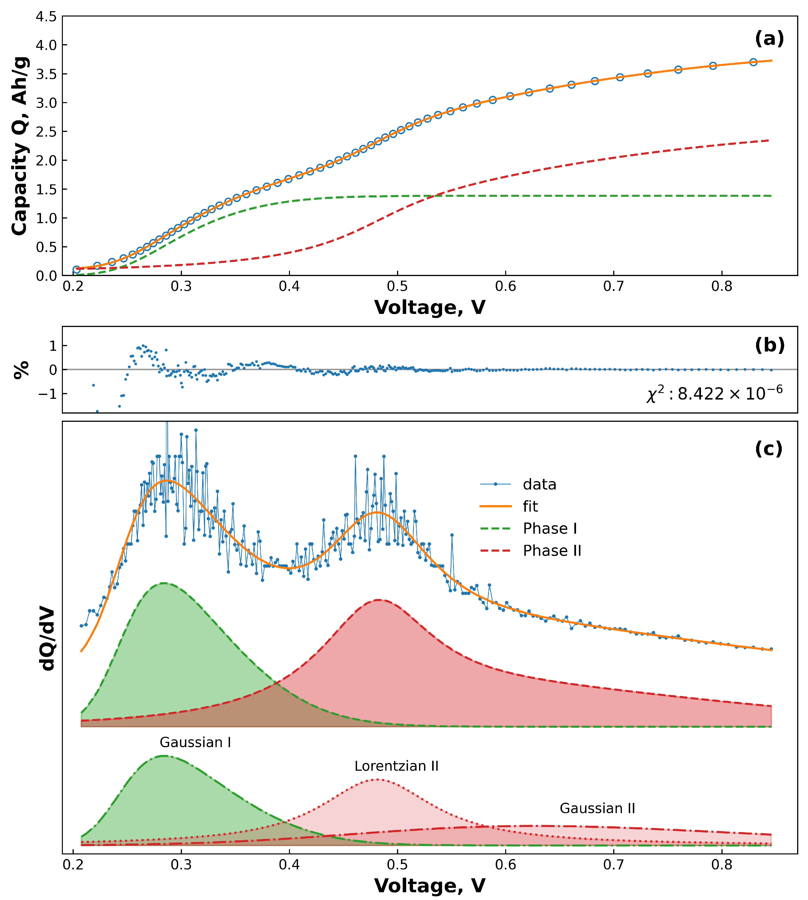
3.1. Parameter Setup and Goodness of Fit

The initial parameter setup for fitting is set according to the known behaviour of Si during delithiation. The alloying phases of Si during lithiation and delithiation have been determined by NMR and PDF, and it has been shown that Si forms amorphous or crystalline phases depending on cycling conditions [6,23,42]. During delithiation, Li is removed from amorphous Li 3.5 Si in two distinct phases, yielding a value of  n = 2  for Equation (1). The two phases are named I and II, and the parameters of the phases are distinguished using the subscripts I and II, respectively. Phase I (Li 3.5 Si → Li 2 Si) is located at about 0.3 V, while phase II (Li 2 Si → Si) is located at about 0.48 V. From the stoichiometry of these two phases it is also possible to estimate the initial Q parameters, assuming that the material at the beginning of the GCD step consists purely of Li 3.5 Si, and the delithiation is complete (i.e., only Si remains at the end of the cycle). This gives a theoretical stoichiometry of 1.5:2, equivalent to 43% of the capacity coming from phase I, while the remaining 57% comes from phase II.
Figure 1 shows an example of the residual and fit of each phase to a GCD curve, along with the equivalent dQ/dV. Figure 1a shows how the fitting function agrees with the data, along with how the two phases contribute to the total curve. The plot of the residuals in Figure 1b shows an overall excellent fit to the data, with the error not exceeding 1.5%. Analysis of the errors of the individual parameters reveals that the errors are almost all less than 10% of the parameter value, and the majority are below 5%. The exception to this is the parameter c, which due to the small values of c compared to the other parameters, displayed larger errors of up to ten times the parameter value. The equivalent dQ/dV is plotted in Figure 1c, with the bottom set of curves showing how the results of the fit is split into skew-Gaussian and Lorentzian curves. Phase I displays no Lorentzian behaviour, and phase II shows a sharp Lorentzian curve as well as a very broad skew-Gaussian curve. This shows that there is excellent agreement between the shape and position of the phases and the results of the fit equations, and reveals that the model is an accurate representation of the shape of the curve. Further, Figure 1c shows that the shapes of the phases are not symmetric about the position c and that the skewness factor  α  is crucial to accurately describe the behaviour of the delithiation curves.

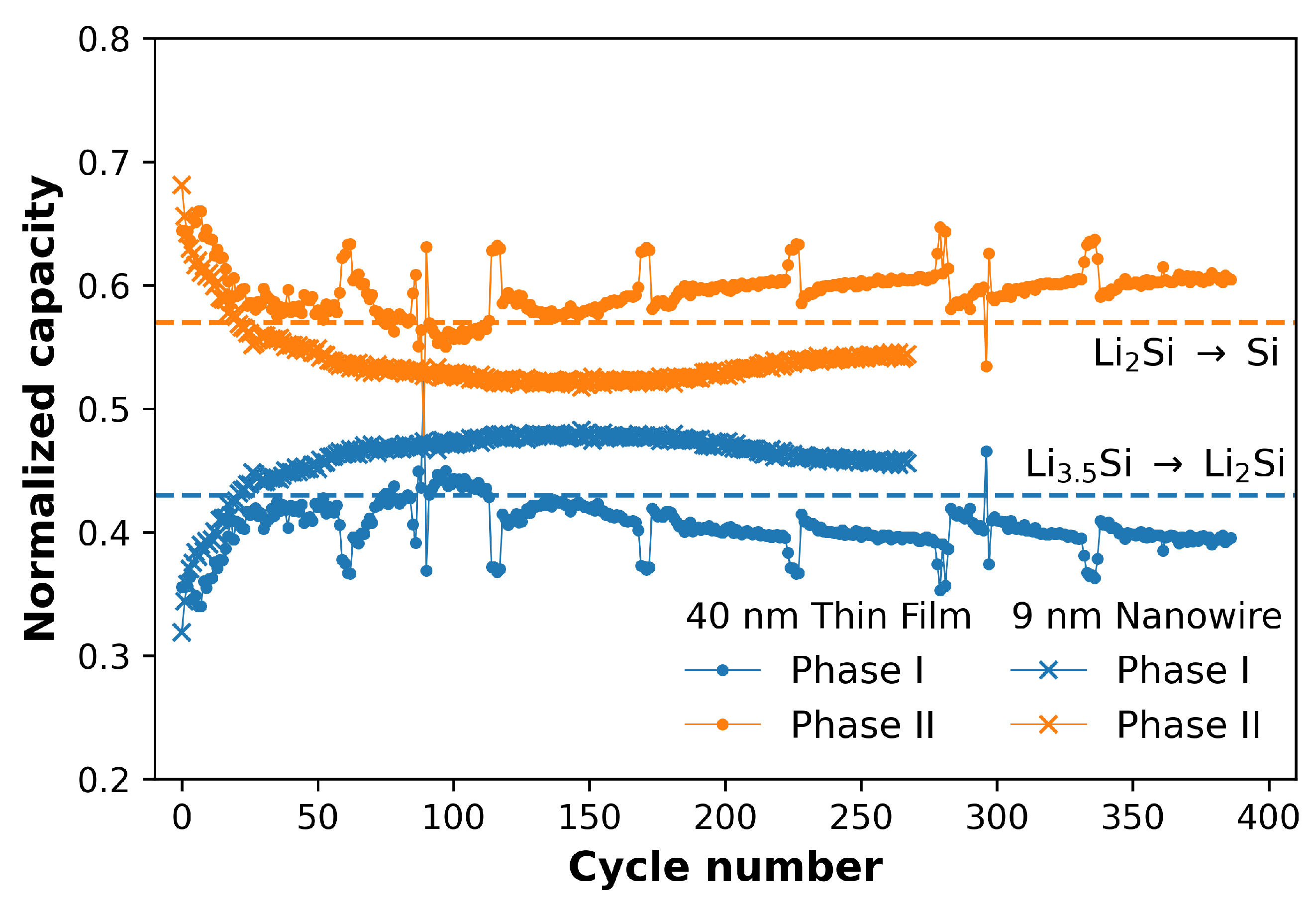
3.2. Comparison of Thin Films and Nanowires

Characterization of the NWs may be found in the original work [16]. The Coulombic efficiencies (CE) of the samples exceeded the 99.5% required for long-term cycling after about 20 cycles. An in-depth discussion of the NW CE is given in the original work [16]. Figure 2 shows how the curves change with repeated cycling for an example of 40 nm TFs (Figure 2a) and 9 nm NWs (Figure 2b). This shows that the individual phases of the two samples behave quite differently, and also shows how important it is to consider the many experimental variables that contribute to cell behaviour. If we were to only look at the complete dQ/dV (grey curves), we might be convinced that both TFs and NWs behave quite similarly. For example, the position of phase I appears to be at about 0.32 V for both samples. However, by looking at the behaviour of only phase I (green curves), it can be seen that this phase is more skewed (higher  α ) for the TF sample than the NW sample. Simultaneously, the position of phase I ( c I , shown as coloured circles on the curves at 0.3 V) is decreasing for the TF sample, but increasing for the NW sample. Note that the position of a phase is not necessarily the point at which the dQ/dV displays a maximum. Similarly, comparing phase II using only the total dQ/dV behaviour would limit us to discussing only the small shift in peak position experienced by the NWs. Instead, by looking at the behaviour of phase II alone (red curves), it can be seen that the Lorentzian portion of the curve is consistently narrower for TFs than for NWs and that the skew-Gaussian portion of phase II is fading slower for TFs than for NWs. This shows that the fitting function provides a powerful tool for analysing the behaviour of Si phases according to their component curves.
As seen in Figure 2, the behaviour of a parameter is affected by all other parameters and it is therefore difficult to separate their behaviour and ascribe meaning to them. Nevertheless, in order to show the changes in the datasets over time, the plots of the individual parameters  α , c, s γ , and w are shown in the SI.
The differences in behaviour of the TFs and NWs shown in Figure 2 give insights into the behaviour of the materials, and can give information about how Equation (1) relates to physical phenomena occurring in the cells. For instance, the increased skewness seen in the phase I peak for TFs (Figure 2a) indicates that there is a relatively large “lagging” effect as the potential increases faster than the diffusion can equilibrate. This is consistent with the expectation that the delithiation is hindered by the long diffusion distance of Li to the surface of the Si. The less skewed phase I NW peak (Figure 2b and Figure S1a) supports this hypothesis, as the thin NWs have lower diffusion lengths, and can diffuse Li in radial directions. The decrease in skewness factor  α I  seen when cycling the TFs at lower C-rates (Figure S1b) further corroborates this, as cycling at rates closer to equilibrium would decrease the diffusion overpotentials. Similarly, the differences in phase position  c I  of phase I give information about two datasets. For thin films, the positions of phase I shift from around 270 to 250 mV over the course of cycling, while NWs show the opposite trend, with the position increasing from 250 to 300 mV. In both cases, however, the positions of  c I  (Figure S2) are very close to the equilibrium potentials determined by the previous literature [6,42,43]. This might indicate that the overpotentials are increasing with cycling in the case of NWs but not TFs, but given that the overpotentials in TFs would also be expected to increase, this explanation alone provides an incomplete picture of the behaviour of  c I . Rather, the exact position of  c I  is likely decided by the combination of diffusion effects described by  α I , and the growing iR drop encroaching on the phase. Since  α I  is relatively stable for TFs, pushing the “start” of the data to higher voltages forces the fitting function to compensate by shifting  c I  to lower values. Conversely, the decreasing  α I  seen for NWs causes  c I  to shift to the right. It is therefore clear that  c I  is not a simple function of the equilibrium potential, but is affected by the behaviour of the cell at the very start of the cycle. It would therefore be more correct to deem c an “apparent” equilibrium potential [6,14,23,44].
Finally, the scale parameter  s I  gives information about how fast the delithiation is occurring in phase I [25]. While the total dQ/dV (grey curves, Figure 2a,b) seem to show that the width of the phase may be slightly narrower for TFs than NWs (Figure 2a and Figure 2b, respectively), the output of the fitting shows that the opposite is true (Figure S3). Further, the slower TF cycles in Figure S3b show lower values of  s I , indicating that the resistance to delithiation described by the skew-Gaussian component is dependent on the C-rate. This behaviour matches the expectation that as the applied current is reduced, the overpotentials will also be reduced [45]. This result matches the expectation that the thinner NWs should delithiate faster (relative to the applied current) than the thicker TFs due both to the decreased diffusion distance as well as the slower C-rates.
As with phase I, analysis of phase II gives important information about the behaviour of Si. Notably,  c I I  is independent of TF thickness, and only slightly decreased at slower C-rates (Figure S2b), varying from 460 to 480 mV. Meanwhile,  c I I  (shown as diamonds on the curves in Figure 2) for the NWs shows a small shift from 460 to 500 mV at the start of cycling before reaching a steady state. This initial increase could be due to an increase in overpotentials due to SEI formation in early cycles. The shift to lower potentials seen in phase I is not reflected in phase II because the position of phase II is relatively close to the middle of the dataset. Hence, there are enough datapoints at low voltages to adequately describe the curve. While phase I is described only by the skew-Gaussian component ( w = 1 ), phase II is described by a combination of both the skew-Gaussian and Lorentzian components. Due to  α I I , the contribution to capacity of the Lorentzian occurs earlier in the delithiation, and the contribution of the skew-Gaussian component is only significant after the maximum of the Lorentzian has been reached. The resulting behaviour indicates a relatively fast “burst” of delithiation described by the Lorentzian, followed by a slower “tail” described by the skew-Gaussian. As with the scale parameter s of the skew-Gaussian, the scale parameter  γ  of the Lorentzian also gives information about how quickly the reaction is occurring. However, unlike the behaviour seen for  s I γ I I  is larger for NWs than for TFs (Figure S4a and S4b, respectively). This would indicate an increase in resistance to delithiation of the NWs compared to the TFs. As cycling progresses, the position of the phase is shifted to higher voltages due to increasing overpotentials, but the onset of delithiation (visible at around 0.25 V in Figure 2) remains constant. The result is that  γ I I  increases to cover the larger potential range over which the phase occurs.
The skew-Gaussian component of phase II describes the end behaviour of the delithiation. As with  α I α I I  is smaller for NWs than TFs (Figure S1a and S1b, respectively). This again matches the expectation that the diffusion of Li in the TFs takes longer due to the dimensionality and thickness of the materials. Similarly,  s I I  shows the same trend as  s I , and we can conclude that delithiation of phase II is hindered by the slow diffusion in the same way as for phase I.
When considering the behaviour of phase II, it is important to bear in mind the relative contribution to the phase of each component. The weighting parameter w determines whether the phase is “skew-Gaussian-limited” ( w 1 ) or “Lorentzian-limited” ( w 0 ). For the Si morphologies studied here,  w I  was always found to be 1. This indicates that the capacity of this phase is skew-Gaussian-limited, at least within the C-rates studied. Figure S5 shows the behaviour of parameter  w I I  for phase II TFs and NWs. From this plot, it can be seen that w for TFs remains stable at around 0.5 during normal cycling, while for the NWs w begins at 0.45 and trends towards 0. This means that the resistances in the TFs are not dominated by either the skew-Gaussian nor the Lorentzian parameters, but the NWs are increasingly limited by the Lorentzian. This difference could be explained by the shrinking of the NWs during delithiation coupled with the growth of SEI in the electrode during cycling. This results in a loss of electrical contact between NWs and leads to a progressive increase in resistance greater than that experienced by the TFs. This hypothesis is supported by the fact that  w I = 1  for all samples and morphologies tested because the highly lithiated Li 3.5 Si phase is about 3.5 times more conductive than the Li 2 Si phase, which is sufficient to overcome the SEI-related resistances [46].

3.3. Phases of Si Delithiation

To further highlight the ability of this method to show differences between the datasets in ways that are not obvious by dQ/dV, the capacities of the two phases normalized to the total capacity determined by the fitting are shown in Figure 3. The horizontal dotted lines denote the initial guesses for the fitting of the phases as discussed in Section 3.1. While this shows that the assumption made initially, i.e., that the datasets consist of 100% Li 3.5 Si at the start of delithiation and 100% Si at the end of delithiation, was not completely accurate, the fitting reveals interesting differences between the TF and NW samples. For both TFs and NWs, the first 10 to 20 cycles show an increase in the contribution to the total capacity from phase I. However, while phase I for the TFs contributes less capacity than expected throughout cycling, the capacity contribution from phase I for the NWs continues to increase and eventually exceeds the amount of capacity expected from the initial assumption made in Section 3.1. The initial increase in contribution from phase I can be explained by the progressive lithiation of Si at the start of repeated cycling proposed in the literature [19,20,47]. In this case, the resistance to lithiation of fresh Si electrodes results in the incomplete conversion of Li 2 Si → Li 3.5 Si during lithiation. This means that at the start of the delithiation step the Si consists of a mixture of Li 3.5 Si and Li 2 Si, and results in less capacity contribution from phase I during delithiation, and more from phase II.
The differences between the TFs and NWs at later cycles can be explained by differences in morphology and C-rate. With repeated cycling, the NWs experience more pronounced SEI growth than the TFs, and therefore increased electrode resistance. This causes the voltage cut-off of the delithiation step to be reached sooner, leading to incomplete delithiation of phase II to form Si, and a disproportionately large contribution to capacity from phase I. This agrees with the observation in Figure 2b that  c I  is shifting to higher potentials. For TFs, the SEI growth occurs relatively slowly (compared to the NWs) and so the electrode resistance plays a less important role. Instead, the larger Li ion diffusion length experienced by the relatively thick TFs, combined with the faster C-rate used for cycling, leads to incomplete formation of Li 3.5 Si during lithiation. This means that, as with the first 10–20 cycles, the electrode consists of a mixture of Li 3.5 Si and Li 2 Si rather than just Li 3.5 Si, and the amount of capacity extracted from phase II is increased.

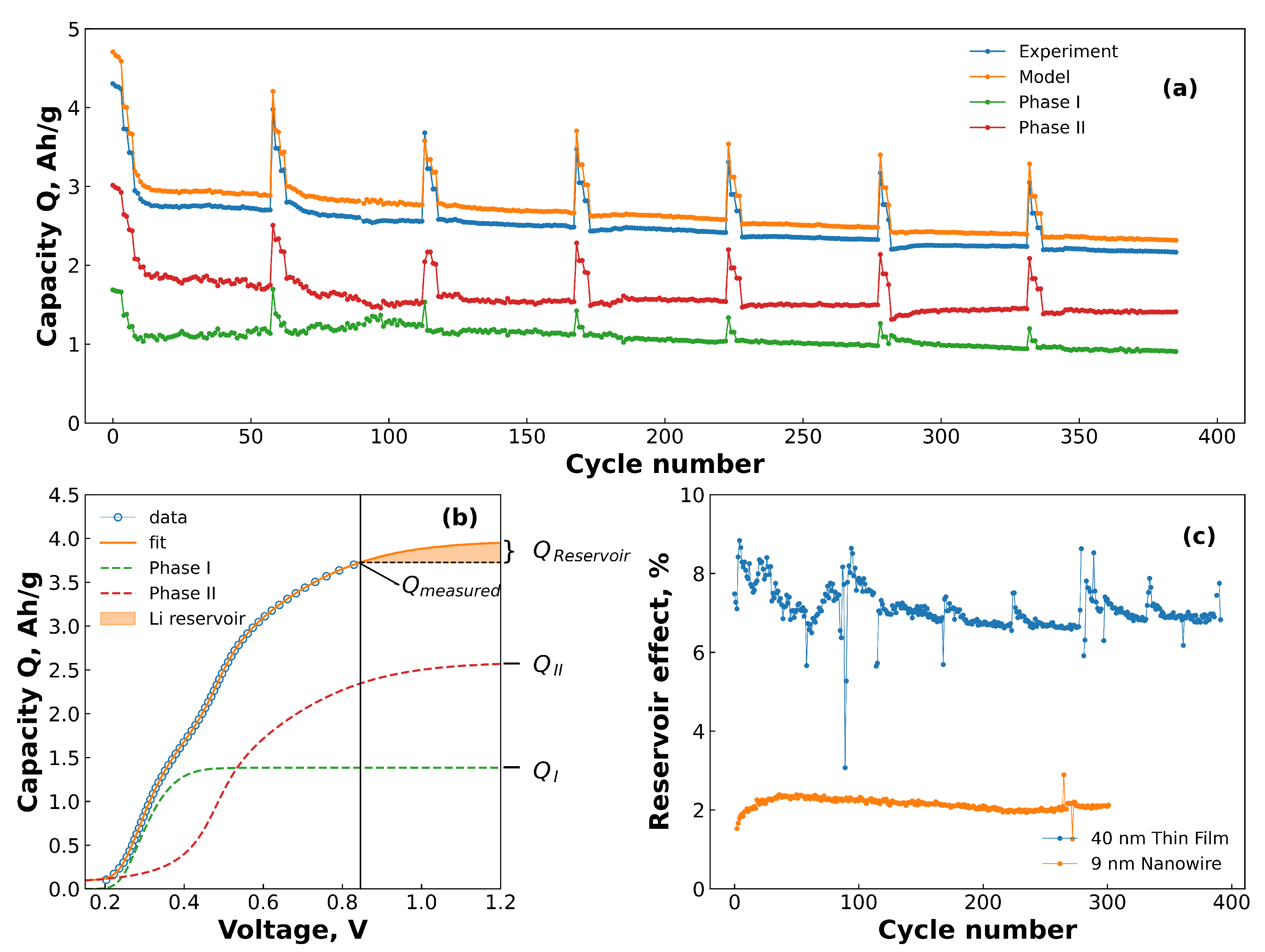
3.4. Voltage Slippage and Excess Li Effects

To demonstrate how well the fitting function describes the data with repeated cycling, an example of the capacities of the each of the two phases, along with the experimentally measured capacity and the total capacity output by the model are given in Figure 4a as a function of the cycle number. It can be seen that the model consistently overestimates the total capacity of the cell. This is because as the slope of the voltage–capacity curve is not 0 at the cut-off potential, indicating that the cell is not fully delithiated at the end of the cycle. This extra capacity has previously been described as a “reservoir effect”, made up of unreleased Li and voltage slippage effects [48]. The size of this reservoir can be estimated from the results of the fit by the simple relation:
Q r e s e r v o i r = Q m o d e l Q m e a s u r e d
where
Q m o d e l = Q I + Q I I
Using these formulae, it is therefore possible to calculate the size of the reservoir effect in the electrode and follow its behaviour with time. Figure 4b shows schematically how the reservoir starts to grow after the voltage cut-off (black line) until it reaches a steady value when  Q r e s e r v o i r  stops increasing. Figure 4c shows the results of applying Equation (2) to the results from the two datasets, plotted as a percentage of the measured capacity ( Q r e s e r v o i r / Q m e a s u r e d ). From this plot it can be seen that the size of the reservoir is strongly dependent on the morphology, with the NWs averaging about 2%, while the TFs maintain a relatively stable reservoir of about 7% of the measured capacity. However, it should be emphasised that the C-rates used to generate data for the two morphologies were not the same, with the TFs cycling at a C-rate 2.5x greater than the NWs. This will likely also contribute to the difference as the TFs have less time to delithiate fully, resulting in a larger reservoir. Nevertheless, the ability of the fitting function to discern these differences and estimate the size of the reservoir is quite valuable.

4. Conclusions

Two datasets of previously published data consisting of delithiation cycling data from a thin film and a nanowire study performed by different groups, were analysed using an empirical cumulative distribution function consisting of a skewed pseudo-Voigt. Both datasets featured Si half-cells cycled in the amorphous region of Si and the skewed pseudo-Voigt was applied to each of the two electrochemical phases Li 3.5 Si (phase I) and Li 2 Si (phase II). The fitting function was found to give excellent fits to both datasets at C-rates far above equilibrium conditions, and was able to determine differences and similarities between the two morphologies studied. Phase I of the NW samples were found to be less skewed than the TFs, indicating faster delithiation. However, loss of contact between NWs and excess SEI growth also lead to increased resistances of the electrodes, in particular for the less electronically conductive phase II. Analysis of the results showed that the fitting function could determine the contribution to capacity of each of the two phases involved in the delithiation of amorphous Si and showed that this is strongly dependent on morphology and cycling rates, with NW electrodes exhibiting lower contribution to capacity than expected from phase II due to greater electrode resistance, despite the larger surface area available for delithiation. Further, the results were shown to be useful in determining the extent of the reservoir effect of the cells, and showed that the thin films exhibited a greater reservoir at the end of the delithiation step compared to the nanowires. This was presumed to be due in part to the greater delithiation path length, and partly to the higher C-rate used in cycling. In conclusion, the fitting function shows promise as a tool to extract more information from Si cycling data even if that data is not generated with the express goal of fitting, and we invite other researchers to apply this method to their past and future data.

Supplementary Materials

The following supporting information can be downloaded at: https://www.mdpi.com/article/10.3390/batteries9050251/s1. Figure S1: The skew parameter  α  for phases I and II for (a) NWs and (b) TFs, as a function of the cycle life; Figure S2 The equilibrium potential c for phases I and II for (a) NWs and (b) TFs, plotted as a function of the cycle life; Figure S3: The scale parameter s of the Gaussian component for phases I and II for (a) NWs and (b) TFs, plotted as a function of the cycle life; Figure S4: The scale parameter  λ  of the Lorentzian component for phase I for (a) NWs and (b) TFs, plotted as a function of the cycle life; Figure S5: The weighting parameter w for phases I and II for (a) NWs and (b) TFs, as a function of the cycle life.

Author Contributions

Conceptualization, F.T.H.; Methodology, F.T.H. and J.P.M.; Software, F.T.H.; Validation, F.T.H., C.K., J.P.M. and O.E.E.; Formal Analysis, F.T.H.; Investigation, F.T.H.; Data Curation, F.T.H., C.K., S.Y.L., A.Y.K. and J.P.M.; Writing—Original Draft Preparation, F.T.H.; Writing—Review and Editing, F.T.H., C.K., J.P.M., O.E.E., S.Y.L., A.Y.K. and Z.Y.; Visualization, F.T.H.; Supervision, F.L. and Z.Y.; Project Administration, F.L.; Funding Acquisition, F.L. All authors have read and agreed to the published version of the manuscript.

Funding

This research was funded by the Research Council of Norway grant number 304644.

Institutional Review Board Statement

Not applicable.

Informed Consent Statement

Not applicable.

Data Availability Statement

Data is available upon reasonable request.

Acknowledgments

The authors acknowledge Rasim Batmaz and Jørn Døvling of Beyonder for their advice and many useful discussions. The thin film electrochemical experiments were funded by the Research Council of Norway through the ENERGIX Project No. 280985, and performed within MoZEES, a Norwegian Centre for Environment-friendly Energy Research (FME), co-sponsored by the Research Council of Norway (project number 257653) and 40 partners from research, industry, and the public sector. The authors would also like to thank Pascale Chenevier for her advice on SiNWs.

Conflicts of Interest

F.T.H., O.E.E. and F.L. declare that they are employees of Beyonder AS, a Norwegian battery manufacturer. F.T.H. and F.L. further declare that they own stock in Beyonder AS. The remaining authors do not declare a conflict of interest.

References

  1. Yin, Y.; Wan, L.; Guo, Y. Silicon-Based Nanomaterials for Lithium-Ion Batteries. Chin. Sci. Bull. 2012, 57, 4104–4110. [Google Scholar] [CrossRef] [Green Version]
  2. McDowell, M.T.; Lee, S.W.; Nix, W.D.; Cui, Y. 25th Anniversary Article: Understanding the Lithiation of Silicon and Other Alloying Anodes for Lithium-Ion Batteries. Adv. Mater. 2013, 25, 4966–4985. [Google Scholar] [CrossRef] [PubMed]
  3. Li, P.; Zhao, G.; Zheng, X.; Xu, X.; Yao, C.; Sun, W.; Dou, S.X. Recent Progress on Silicon-Based Anode Materials for Practical Lithium-Ion Battery Applications. Energy Storage Mater. 2018, 15, 422–446. [Google Scholar] [CrossRef]
  4. Bloom, I.; Jansen, A.N.; Abraham, D.P.; Knuth, J.; Jones, S.A.; Battaglia, V.S.; Henriksen, G.L. Differential Voltage Analyses of High-Power, Lithium-Ion Cells 1. J. Power Sources 2005, 139, 295–303. [Google Scholar] [CrossRef]
  5. Chevrier, V.L.; Zwanziger, J.W.; Dahn, J.R. First Principles Studies of Silicon as a Negative Electrode Material for Lithium-Ion Batteries. Can. J. Phys. 2009, 87, 625–632. [Google Scholar] [CrossRef]
  6. Ogata, K.; Salager, E.; Kerr, C.; Fraser, A.; Ducati, C.; Morris, A.; Hofmann, S.; Grey, C. Revealing Lithium–Silicide Phase Transformations in Nano-Structured Silicon-Based Lithium Ion Batteries via in Situ NMR Spectroscopy. Nat. Commun. 2014, 5, 3217. [Google Scholar] [CrossRef] [Green Version]
  7. Chevrier, V.L.; Liu, L.; Wohl, R.; Chandrasoma, A.; Vega, J.A.; Eberman, K.W.; Stegmaier, P.; Figgemeier, E. Design and Testing of Prelithiated Full Cells with High Silicon Content. J. Electrochem. Soc. 2018, 165, A1129–A1136. [Google Scholar] [CrossRef]
  8. Kitada, K.; Pecher, O.; Magusin, P.C.M.M.; Groh, M.F.; Weatherup, R.S.; Grey, C.P. Unraveling the Reaction Mechanisms of SiO Anodes for Li-Ion Batteries by Combining In Situ 7 Li and Ex Situ 7 Li/ 29 Si Solid-State NMR Spectroscopy. J. Am. Chem. Soc. 2019, 141, 7014–7027. [Google Scholar] [CrossRef]
  9. Beaulieu, L.Y.; Hatchard, T.D.; Bonakdarpour, A.; Fleischauer, M.D.; Dahn, J.R. Reaction of Li with Alloy Thin Films Studied by In Situ AFM. J. Electrochem. Soc. 2003, 150, A1457. [Google Scholar] [CrossRef]
  10. Limthongkul, P.; Jang, Y.I.; Dudney, N.J.; Chiang, Y.M. Electrochemically-Driven Solid-State Amorphization in Lithium-Silicon Alloys and Implications for Lithium Storage. Acta Mater. 2003, 51, 1103–1113. [Google Scholar] [CrossRef]
  11. Obrovac, M.N.; Krause, L.J. Reversible Cycling of Crystalline Silicon Powder. J. Electrochem. Soc. 2007, 154, A103. [Google Scholar] [CrossRef]
  12. Wang, M.; Xiao, X.; Huang, X. Study of Lithium Diffusivity in Amorphous Silicon via Finite Element Analysis. J. Power Sources 2016, 307, 77–85. [Google Scholar] [CrossRef] [Green Version]
  13. Swamy, T.; Chiang, Y.M. Electrochemical Charge Transfer Reaction Kinetics at the Silicon-Liquid Electrolyte Interface. J. Electrochem. Soc. 2015, 162, A7129–A7134. [Google Scholar] [CrossRef]
  14. Sethuraman, V.A.; Srinivasan, V.; Newman, J. Analysis of Electrochemical Lithiation and Delithiation Kinetics in Silicon. J. Electrochem. Soc. 2013, 160, A394–A403. [Google Scholar] [CrossRef]
  15. Lai, S.Y.; Mæhlen, J.P.; Preston, T.J.; Skare, M.O.; Nagell, M.U.; Ulvestad, A.; Lemordant, D.; Koposov, A.Y. Morphology Engineering of Silicon Nanoparticles for Better Performance in Li-ion Battery Anodes. Nanoscale Adv. 2020, 2, 5335–5342. [Google Scholar] [CrossRef]
  16. Keller, C.; Desrues, A.; Karuppiah, S.; Martin, E.; Alper, J.; Boismain, F.; Villevieille, C.; Herlin-Boime, N.; Haon, C.; Chenevier, P. Effect of Size and Shape on Electrochemical Performance of Nano-Silicon-Based Lithium Battery. Nanomaterials 2021, 11, 307. [Google Scholar] [CrossRef] [PubMed]
  17. Alvarez Barragan, A.; Nava, G.; Wagner, N.J.; Mangolini, L. Silicon-Carbon Composites for Lithium-Ion Batteries: A Comparative Study of Different Carbon Deposition Approaches. J. Vac. Sci. Technol. Nanotechnol. Microelectron. Mater. Process. Meas. Phenom. 2018, 36, 011402. [Google Scholar] [CrossRef]
  18. Bernard, P.; Alper, J.P.; Haon, C.; Herlin-Boime, N.; Chandesris, M. Electrochemical Analysis of Silicon Nanoparticle Lithiation—Effect of Crystallinity and Carbon Coating Quantity. J. Power Sources 2019, 435, 226769. [Google Scholar] [CrossRef]
  19. Huld, F.T.; Lai, S.Y.; Tucho, W.M.; Batmaz, R.; Jensen, I.T.; Lu, S.; Eleri, O.E.; Koposov, A.Y.; Yu, Z.; Lou, F. Enabling Increased Delithiation Rates in Silicon-Based Anodes through Alloying with Phosphorus. ChemistrySelect 2022, 7, e202202857. [Google Scholar] [CrossRef]
  20. Ulvestad, A.; Skare, M.O.; Foss, C.E.; Krogsæter, H.; Reichstein, J.F.; Preston, T.J.; Mæhlen, J.P.; Andersen, H.F.; Koposov, A.Y. Stoichiometry-Controlled Reversible Lithiation Capacity in Nanostructured Silicon Nitrides Enabled by In Situ Conversion Reaction. ACS Nano 2021, 15, 16777–16787. [Google Scholar] [CrossRef]
  21. Chen, L.; Xie, X.; Xie, J.; Wang, K.; Yang, J. Binder Effect on Cycling Performance of Silicon/Carbon Composite Anodes for Lithium Ion Batteries. J. Appl. Electrochem. 2006, 36, 1099–1104. [Google Scholar] [CrossRef]
  22. Huang, L.H.; Li, C.C. Effects of Interactions between Binders and Different-Sized Silicons on Dispersion Homogeneity of Anodes and Electrochemistry of Lithium-Silicon Batteries. J. Power Sources 2019, 409, 38–47. [Google Scholar] [CrossRef]
  23. Li, J.; Dahn, J.R. An In Situ X-ray Diffraction Study of the Reaction of Li with Crystalline Si. J. Electrochem. Soc. 2007, 154, A156. [Google Scholar] [CrossRef]
  24. McDowell, M.T.; Ryu, I.; Lee, S.W.; Wang, C.; Nix, W.D.; Cui, Y. Studying the Kinetics of Crystalline Silicon Nanoparticle Lithiation with In Situ Transmission Electron Microscopy. Adv. Mater. 2012, 24, 6034–6041. [Google Scholar] [CrossRef] [PubMed]
  25. Olson, J.Z.; López, C.M.; Dickinson, E.J.F. Differential Analysis of Galvanostatic Cycle Data from Li-Ion Batteries: Interpretative Insights and Graphical Heuristics. Chem. Mater. 2023, 35, 1487–1513. [Google Scholar] [CrossRef]
  26. Palagonia, M.S.; Erinmwingbovo, C.; Brogioli, D.; La Mantia, F. Comparison between Cyclic Voltammetry and Differential Charge Plots from Galvanostatic Cycling. J. Electroanal. Chem. 2019, 847, 113170. [Google Scholar] [CrossRef]
  27. Dubarry, M.; Truchot, C.; Liaw, B.Y. Cell Degradation in Commercial LiFePO4 Cells with High-Power and High-Energy Designs. J. Power Sources 2014, 258, 408–419. [Google Scholar] [CrossRef]
  28. Dubarry, M.; Liaw, B.Y. Identify Capacity Fading Mechanism in a Commercial LiFePO4 Cell. J. Power Sources 2009, 194, 541–549. [Google Scholar] [CrossRef]
  29. Dubarry, M.; Liaw, B.Y.; Chen, M.S.; Chyan, S.S.; Han, K.C.; Sie, W.T.; Wu, S.H. Identifying Battery Aging Mechanisms in Large Format Li Ion Cells. J. Power Sources 2011, 196, 3420–3425. [Google Scholar] [CrossRef]
  30. Li, Y.; Abdel-Monem, M.; Gopalakrishnan, R.; Berecibar, M.; Nanini-Maury, E.; Omar, N.; van den Bossche, P.; Van Mierlo, J. A Quick On-Line State of Health Estimation Method for Li-ion Battery with Incremental Capacity Curves Processed by Gaussian Filter. J. Power Sources 2018, 373, 40–53. [Google Scholar] [CrossRef]
  31. Li, X.; Wang, Z.; Yan, J. Prognostic Health Condition for Lithium Battery Using the Partial Incremental Capacity and Gaussian Process Regression. J. Power Sources 2019, 421, 56–67. [Google Scholar] [CrossRef]
  32. He, J.; Bian, X.; Liu, L.; Wei, Z.; Yan, F. Comparative Study of Curve Determination Methods for Incremental Capacity Analysis and State of Health Estimation of Lithium-Ion Battery. J. Energy Storage 2020, 29, 101400. [Google Scholar] [CrossRef]
  33. Yoon, T.; Nguyen, C.C.; Seo, D.M.; Lucht, B.L. Capacity Fading Mechanisms of Silicon Nanoparticle Negative Electrodes for Lithium Ion Batteries. J. Electrochem. Soc. 2015, 162, A2325–A2330. [Google Scholar] [CrossRef] [Green Version]
  34. Thompson, N.; Cohen, T.; Alamdari, S.; Hsu, C.W.; Williamson, G.; Beck, D.; Holmberg, V. DiffCapAnalyzer: A Python Package for Quantitative Analysis of Total Differential Capacity Data. J. Open Source Softw. 2020, 5, 2624. [Google Scholar] [CrossRef]
  35. Li, X.; Jiang, J.; Wang, L.Y.; Chen, D.; Zhang, Y.; Zhang, C. A Capacity Model Based on Charging Process for State of Health Estimation of Lithium Ion Batteries. Appl. Energy 2016, 177, 537–543. [Google Scholar] [CrossRef]
  36. Bian, X.; Liu, L.; Yan, J. A Model for State-of-Health Estimation of Lithium Ion Batteries Based on Charging Profiles. Energy 2019, 177, 57–65. [Google Scholar] [CrossRef]
  37. Pang, H.; Guo, L.; Wu, L.; Jin, J.; Zhang, F.; Liu, K. A Novel Extended Kalman Filter-Based Battery Internal and Surface Temperature Estimation Based on an Improved Electro-Thermal Model. J. Energy Storage 2021, 41, 102854. [Google Scholar] [CrossRef]
  38. Pang, H.; Wu, L.; Liu, J.; Liu, X.; Liu, K. Physics-Informed Neural Network Approach for Heat Generation Rate Estimation of Lithium-Ion Battery under Various Driving Conditions. J. Energy Chem. 2023, 78, 1–12. [Google Scholar] [CrossRef]
  39. Sivonxay, E.; Aykol, M.; Persson, K.A. The Lithiation Process and Li Diffusion in Amorphous SiO2 and Si from First-Principles. Electrochim. Acta 2020, 331, 135344. [Google Scholar] [CrossRef]
  40. Hasa, I.; Haregewoin, A.M.; Zhang, L.; Tsai, W.Y.; Guo, J.; Veith, G.M.; Ross, P.N.; Kostecki, R. Electrochemical Reactivity and Passivation of Silicon Thin-Film Electrodes in Organic Carbonate Electrolytes. ACS Appl. Mater. Interfaces 2020, 12, 40879–40890. [Google Scholar] [CrossRef]
  41. Ulvestad, A.; Mæhlen, J.P.; Kirkengen, M. Silicon Nitride as Anode Material for Li-ion Batteries: Understanding the SiNx Conversion Reaction. J. Power Sources 2018, 399, 414–421. [Google Scholar] [CrossRef]
  42. Key, B.; Morcrette, M.; Tarascon, J.M.; Grey, C.P. Pair Distribution Function Analysis and Solid State NMR Studies of Silicon Electrodes for Lithium Ion Batteries: Understanding the (De)Lithiation Mechanisms. J. Am. Chem. Soc. 2011, 133, 503–512. [Google Scholar] [CrossRef] [PubMed]
  43. Tritsaris, G.A.; Zhao, K.; Okeke, O.U.; Kaxiras, E. Diffusion of Lithium in Bulk Amorphous Silicon: A Theoretical Study. J. Phys. Chem. C 2012, 116, 22212–22216. [Google Scholar] [CrossRef]
  44. Ulvestad, A.; Andersen, H.F.; Jensen, I.J.T.; Mongstad, T.T.; Mæhlen, J.P.; Prytz, Ø.; Kirkengen, M. Substoichiometric Silicon Nitride—An Anode Material for Li-ion Batteries Promising High Stability and High Capacity. Sci. Rep. 2018, 8, 8634. [Google Scholar] [CrossRef] [Green Version]
  45. Fly, A.; Chen, R. Rate Dependency of Incremental Capacity Analysis (dQ/dV) as a Diagnostic Tool for Lithium-Ion Batteries. J. Energy Storage 2020, 29, 101329. [Google Scholar] [CrossRef]
  46. Pollak, E.; Salitra, G.; Baranchugov, V.; Aurbach, D. In Situ Conductivity, Impedance Spectroscopy, and Ex Situ Raman Spectra of Amorphous Silicon during the Insertion/Extraction of Lithium. J. Phys. Chem. C 2007, 111, 11437–11444. [Google Scholar] [CrossRef]
  47. Foss, C.E.L.; Müssig, S.; Svensson, A.M.; Vie, P.J.S.; Ulvestad, A.; Mæhlen, J.P.; Koposov, A.Y. Anodes for Li-ion Batteries Prepared from Microcrystalline Silicon and Enabled by Binder’s Chemistry and Pseudo-Self-Healing. Sci. Rep. 2020, 10, 13193. [Google Scholar] [CrossRef]
  48. Rodrigues, M.T.F. Capacity and Coulombic Efficiency Measurements Underestimate the Rate of SEI Growth in Silicon Anodes. J. Electrochem. Soc. 2022, 169, 080524. [Google Scholar] [CrossRef]
Figure 1. An example of the goodness of fit of cycle number 5 from a 40 nm SiTF cell. (a) The raw output of the fitting model, showing the input data as blue points overlaid with the best-fit determined by the program (orange line). The dotted lines are the curves of the individual phases which together make up the full fitting function. (b) Residuals of the fit, displayed as a percentage difference from the measured points. (c) The data from (a), displayed as a dQ/dV plot. The top offset shows the data as blue points overlaid with the best fit (orange line). The middle offset shows the contribution to the fit of phase I (green) and phase II (red). The bottom offset shows how the phases are composed of skew-Gaussian and Lorentzian curves.
Batteries 09 00251 g001
Figure 2. Output of fitting Equation (1) to the data, displayed as dQ/dV and showing the evolution of the curves with cycling for (a) 40 nm TFs, and (b) 9 nm NWs. Each curve is an average of x cycles, where x is  1 / 10 th  of the total number of cycles. The locations of the dots and diamonds correspond to  c I  and  c I I , respectively. The dotted vertical lines denote c for the first cycles.
Batteries 09 00251 g002
Figure 3. Comparison of the capacities of phases I (blue) and II (orange), for an example of thin films (dots) and nanowires (crosses). The data is normalized to the total capacity of each point as determined by the fitting. The horizontal dotted lines denote the initial guess of full conversion between the two phases.
Batteries 09 00251 g003
Figure 4. (a) An example of the capacity vs. cycle life of a thin film sample (blue points), including the capacity contributions of each phase (green and red points) to the total capacity from the model (orange points). (b) Plot showing the capacity of the cell as the voltage is extended beyond the cut-off potential. The blue dots denote the raw data, while the orange line denotes the best fit. The black vertical line at ∼0.85 V denotes the end of the measured data (i.e., the cut-off potential). The orange shaded area is the reservoir. (c) The reservoir of the different materials as calculated from Equation (2). The data is displayed as a percentage of the  Q m e a s u r e d  for each material.
Batteries 09 00251 g004
Table 1. Physical properties of the Si materials used in this work.
Si MorphologyThickness/ Diameter (nm)Surface Area (m 2 /g)Electrode Density (g/cm 3 )Current Density at 1 C (mA/g)Reference
Nanowire9
42
55
194
108
85
0.42
0.33
0.29
0.52
0.73
0.85
[16]
Thin Film40
60
80
10.7
7.15
5.36
2.3290.033
0.045
0.067
This work
Disclaimer/Publisher’s Note: The statements, opinions and data contained in all publications are solely those of the individual author(s) and contributor(s) and not of MDPI and/or the editor(s). MDPI and/or the editor(s) disclaim responsibility for any injury to people or property resulting from any ideas, methods, instructions or products referred to in the content.

