
A Three-Phase Fundamental Diagram from Three-Dimensional Traffic Data
by
 ,
,
Maria Laura Delle Monache
1, 
Karen Chi
2,
Yong Chen
3,
Paola Goatin
4,
Ke Han
5,
Jing-mei Qiu
6 and
Benedetto Piccoli
7,* 1
University Grenoble Alpes, Inria, CNRS, Grenoble INP, GIPSA-Lab, 38000 Grenoble, France
2
Learning Lab, University of Pennsylvania, Philadelphia, PA 19104, USA
3
Department of Biostatistics, Epidemiology and Informatics (DBEI), University of Pennsylvania, Philadelphia, PA 19104, USA
4
Université Côte d’Azur, Inria, CNRS, LJAD, 06902 Sophia Antipolis, France
5
Institute of System Science and Engineering, Southwest Jiaotong University, Chengdu 611756, China
6
Department of Mathematics, University of Delaware, Newark, DE 19713, USA
7
Department of Mathematical Sciences, Rutgers University-Camden, Camden, NJ 08102, USA
*
Author to whom correspondence should be addressed.
Axioms 2021, 10(1), 17; https://doi.org/10.3390/axioms10010017
Submission received: 5 November 2020
/
Revised: 26 January 2021
/
Accepted: 28 January 2021
/
Published: 7 February 2021
(This article belongs to the Special Issue Differential Models, Numerical Simulations and Applications)
Abstract
:This paper uses empirical traffic data collected from three locations in Europe and the US to reveal a three-phase fundamental diagram with two phases located in the uncongested regime. Model-based clustering, hypothesis testing and regression analyses are applied to the speed–flow–occupancy relationship represented in the three-dimensional space to rigorously validate the three phases and identify their gaps. The finding is consistent across the aforementioned different geographical locations. Accordingly, we propose a three-phase macroscopic traffic flow model and a characterization of solutions to the Riemann problems. This work identifies critical structures in the fundamental diagram that are typically ignored in first- and higher-order models and could significantly impact travel time estimation on highways.
MSC:
35L65; 76A30; 62H301. Introduction
In the last seventy years, many traffic flow models have been developed and researched. Two of the most commonly used macroscopic models are the celebrated first-order Lighthill–Whitham–Richards (LWR) model, [1,2] and the second-order Aw-Rascle–Zhang model [3,4]. In both cases, the so-called Fundamental Diagram (FD) provides a closure of the evolution equations, thus allowing a well-posed theory and well-grounded simulation tools (see [5]). The FD usually refers to the empirically observed flow-occupancy curve, which in mathematical terms refers to the functional relationship between flow and density (modeling counterpart of occupancy) or between average speed of vehicles and density. For macroscopic fluid-dynamic models, there is a rich discussion on FD (see, e.g., [5,6,7,8,9,10]).
In this article, we focus on the FD for single roads by proposing a new approach to study the fundamental relationship among flow, density and speed. We propose novel statistical methodologies to analyze traffic data from fixed sensors, focusing on the three-leg relationships among the flow, density and speed. In particular, rather than considering the FD as a two-quantity relationship (flow–density or speed–density), we analyze data in the three-dimensional space represented by flow, density and speed. This allows us to better exploit the statistical tools, in particular for the analysis of traffic regimes.
We recall that, in equilibrium regimes, the fundamental relationship dictates that traffic measurement points should lie on a three-dimensional surface (see, e.g., [11] Figure 4.1). In reality, observed traffic largely deviates from equilibrium and usually exhibits free and congested phases, with the first corresponding to stable and regular traffic, while the second reflects delays and congestion. Moreover, in the early 2000s, Kerner [12] introduced a tree-phase traffic theory, based on the distinction among free flow, synchronized flow and wide-moving jam. The last two phases are associated with congested traffic.
In this paper, using clustering methodologies, we are able to identify three traffic regimes, which are distinct in a statistically significant fashion. Interestingly, two regimes appear in what is commonly referred to as the free flow traffic and the third corresponds to the congested phase. This analysis does not contradict Kerner’s theory but rather points out that the static/stationary free-flow condition in the FD could exhibit two distinct phases, while the distinction of phases in congested traffic (e.g., Kerner’s model) is mainly dynamic.
The second main empirical result of our paper is the clear evidence of the existence of a gap between the two phases of free flow and the congested one. While the appearance of such gap is best visualized in the 3D representation of the FD relationships, we use the classical flow–density relationship to statistically prove the existence of the gap. The main purpose is to prove the ubiquity (with respect to data collected at different geographical location and on different road types) of the gap in the classical setting and to enable a simpler analysis.
Building on the empirical evidence illustrated thus far, we propose a new three-phase macroscopic model. The LWR model is very popular in the traffic literature due to its simple mathematical representation. However, it has certain modeling limitations especially when it comes to describing complex wave structures such as stop and go waves, phantom jam and capacity drop. To overcome various limitations, Aw-Rascle [3] and independently Zhang [4] proposed a new model with conservation of a modified momentum. This so-called Aw-Rascle–Zhang (ARZ) model can be interpreted as part of a general family called General Second-Order Models (GSOM, see [13]). Such models consist of the usual conservation of mass and the advective transport of a Lagrangian (or single driver) variable, which can represent, for instance, the desired speed of drivers. A recently proposed model of this category is the Collapsed Generalized ARZ model (CGARZ [14]), where the driver speed depends on the Lagrangian variable only in the congested phase. Another line of research focuses on models showing two distinct phases, called the phase transition models [6,8,9].
Our proposed model is a combination of the features offered by the ARZ, CGARZ and phase transition models. Our three-phase model not only has the characteristics of a CGARZ model with a gap among phases when analyzed in the flow–density space, but also exhibits the newly discovered phase when analyzed in the speed–density space. After showing how our model performs in data fitting, we provide a complete characterization of the characteristic curves and the solutions of the Riemann problems. The latter are the building block for solutions to Cauchy problems (see [5]). To sum up, the main novelties and contributions of our paper are as follows:
- Unlike most studies that focus on traffic data from a single source, we use data from multiple geographic locations in Europe and the US and analyze the fundamental relationships among flow, density and speed in the 3D space instead of the commonly adopted two-variable representation of the FD. In addition, we use a set of statistical tools including model-based clustering, hypothesis testing and regression to analyze the traffic data.
- Following the above exercise, we discover three data clusters representing three traffic regimes, two of which are contained in the free-flow phase and the third corresponds to the congested phase. Moreover, we are able to detect a statistically significant gap between the first two regimes and the third one. These findings are validated using multiple data sources, and the main features (regimes and gaps) are consistent across different geographical areas.
- Building on the first two, we propose a new three-phase macroscopic traffic flow model, which exhibits all the characteristics shown by our data analyses and combines the features of the ARZ, CGARZ and phase transition models. A complete characterization of solutions of the Riemann problems is provided.
2. Data Analysis
In this section, we describe the data analyzed in the paper and then present the statistical analysis performed.
2.1. Experimental Data
We consider traffic data collected by static sensors (magnetic coils or radars) located on urban and extra-urban roads and highways. Sensors capture these traffic data regularly over a period of time. The sensor data provide the following aggregated quantities which are measured independently over a short time interval (3–10 min).
- Flux (denoted as f), also known as flow or volume, is the number of vehicles passing through a fixed location per unit of time.
- Velocity (denoted as v) is the average speed of vehicles per unit of time.
- Occupancy (denoted as o) is the percentage of time that a vehicle covers the sensor over the unit time of data collection.
Occupancy acts as a surrogate for the true density of traffic, as true density is practically difficult to capture, although there is some measurement error involved with its calculation. It is know that density and occupancy are correlated at lower densities, but this does not extend to higher densities. The data were collected from three different locations: Rome (Italy), Las Vegas (NV, USA) and Sophia Antipolis (France). The Rome data were provided by ATAC S.p.a. [15] (the municipal society for traffic monitoring and control of Rome) and refer to a road in the city of Rome, Viale del Muro Torto, which links the historical center with the northern area of the city. Data were collected over a period of a week on three sensors. Each collected quantity (occupancy, flow and speed) was aggregated on 1 min intervals. The data from Las Vegas were collected by the Regional Transportation Commission of Southern Nevada (RTC), Freeway and Arterial System of Transportation (FAST) [16]. The data were collected from 50 urban and freeway sensors over a period of five years and aggregated on 10 min intervals. The data from Sophia Antipolis were collected by the Départment des Alpes-Maritimes [17] on two extra-urban sensors over a period of eight months and aggregated over 6 min intervals. For more details on the data, we refer the reader to Appendix A. Despite the fact that the data were aggregated at different intervals, the results, as shown below, are consistent. Since we primarily focused on the three traffic characteristics of flux, velocity and occupancy, we were conveniently positioned to analyze the data in three dimensions, a novel concept and approach that is described in the next section.
2.2. Statistical Tools
2.2.1. Cluster Analysis
Cluster analysis is the classification of data with a previously unknown structure and the partitioning of a dataset into meaningful subsets. Clustering sheds light on hidden or non-intuitive relationships between those data and their attributes. Each cluster contains a group of objects that are more closely related to each other than they would be as objects of other clusters. The concept of distance is thus inherently crucial in the process of cluster analysis, as clusters are grouped based on the results of this measure. Distance serves as a way to evaluate the closeness, as well as dissimilarity, of pairs of observations. There are at least two options to conduct cluster analysis for this traffic data: model-based clustering (e.g., mixture of normals) and non-parametric clustering (e.g., k-means). Although k-means is popular for complex and high-dimensional data, it is generally used for data involving variables of the same scale (hence, more suitable for data with spherical clusters, e.g., Euclidean distance in 3D), whereas our data consist of three variables of different scales. For this reason, model-based clustering has more flexibility in the shape of clusters; for instance, mixture models [18] can identify clusters in the traffic data that were ellipsoidal.
Empirical evaluations on the distributions of the three traffic variables through quantile–quantile (Q-Q) plot, Shapiro test and Box–Cox transformation have suggested that normal distributions are appropriate. Here, we propose the use of a finite mixture model with G multivariate normals [18]. Specifically, denote data with independent trivariate observations (flux, velocity and occupancy) the likelihood for a mixture model with G components is
where i stands for ith observation, and are the density function and model parameters of the kth cluster in the mixture and is the probability that an observation belongs to the kth cluster, subject to the simplex constraint . Such a model can be fitted by the expectation-maximization (EM) algorithm and is implemented by the R package ‘mclust’.
2.2.2. Three Phase Traffic
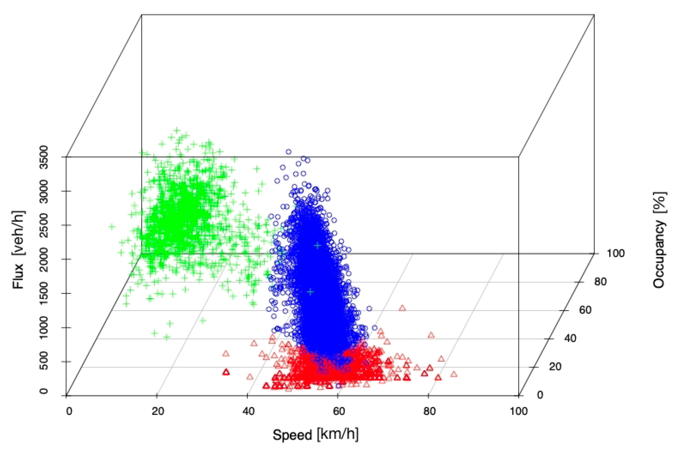
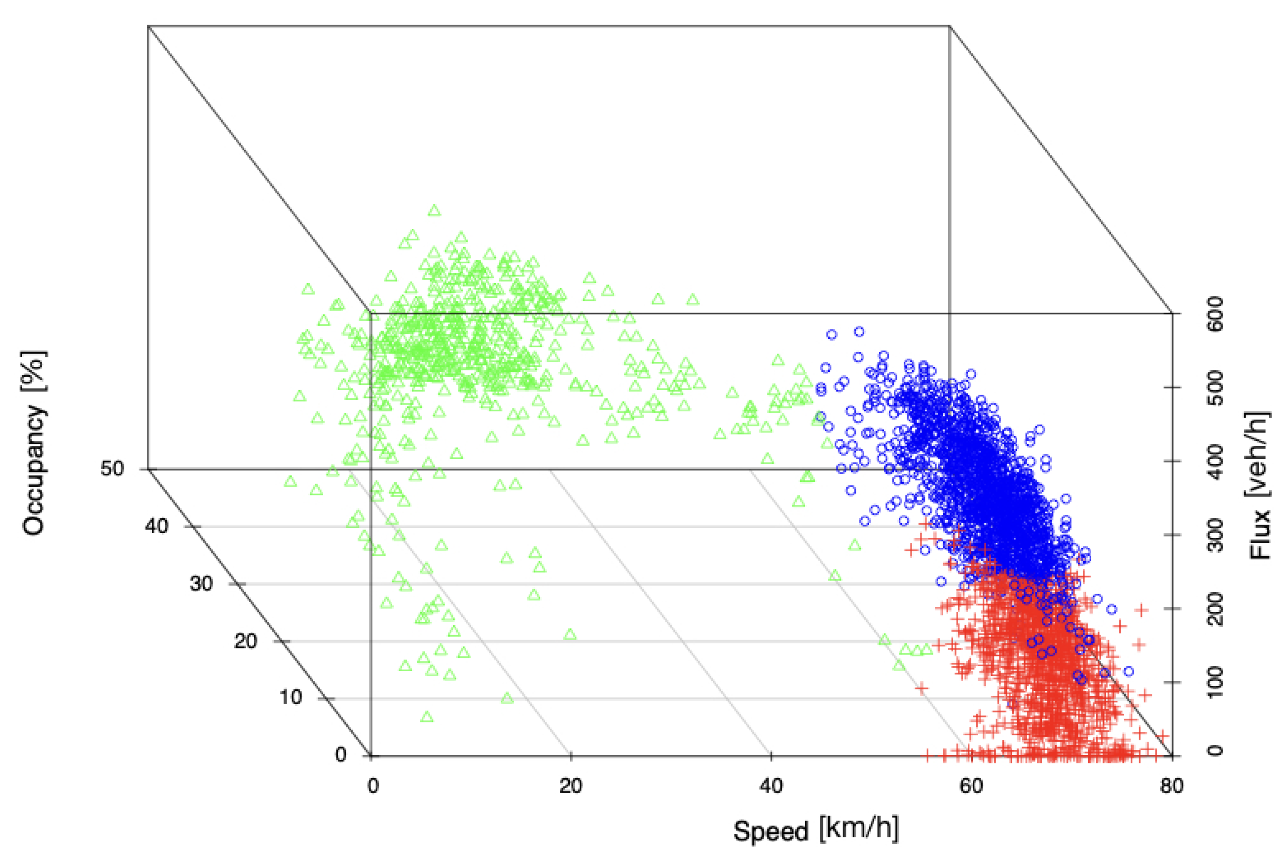
Figure 1 provides a 3D visualization and cluster analysis result on the Rome dataset, where observations in different clusters are marked by different colors. Previous knowledge assumed that traffic involves two clusters: free flow and congestion. Free flow corresponds to steady traffic flow at high speeds (and low densities), while congestion is characterized by low flux and reduced speeds. From this new 3D visualization of data, we can identify a third phase, which we call the “free choice phase”, which corresponds to the situation of a relatively empty road, whereby drivers choose their speed independently without influence from or interaction with other vehicles.
In the free choice phase, the flow of cars is low while the speed is variable. Model selection procedures (e.g., Bayesian information criterion (BIC) or adjusted BIC) have been used to select the number of clusters, and the datasets from Rome, Nevada and Sophia Antipolis have consistently suggested the existence of the third phase. Such additional phase is incorporated into the mathematical modeling.
Notice that our three phases are different from those indicated by Kerner [12]. Indeed, we have two sub-phases in the free phase cluster opposed to Kerner’s model with two sub-phases in the congestion phase cluster.
2.2.3. Gap Analysis
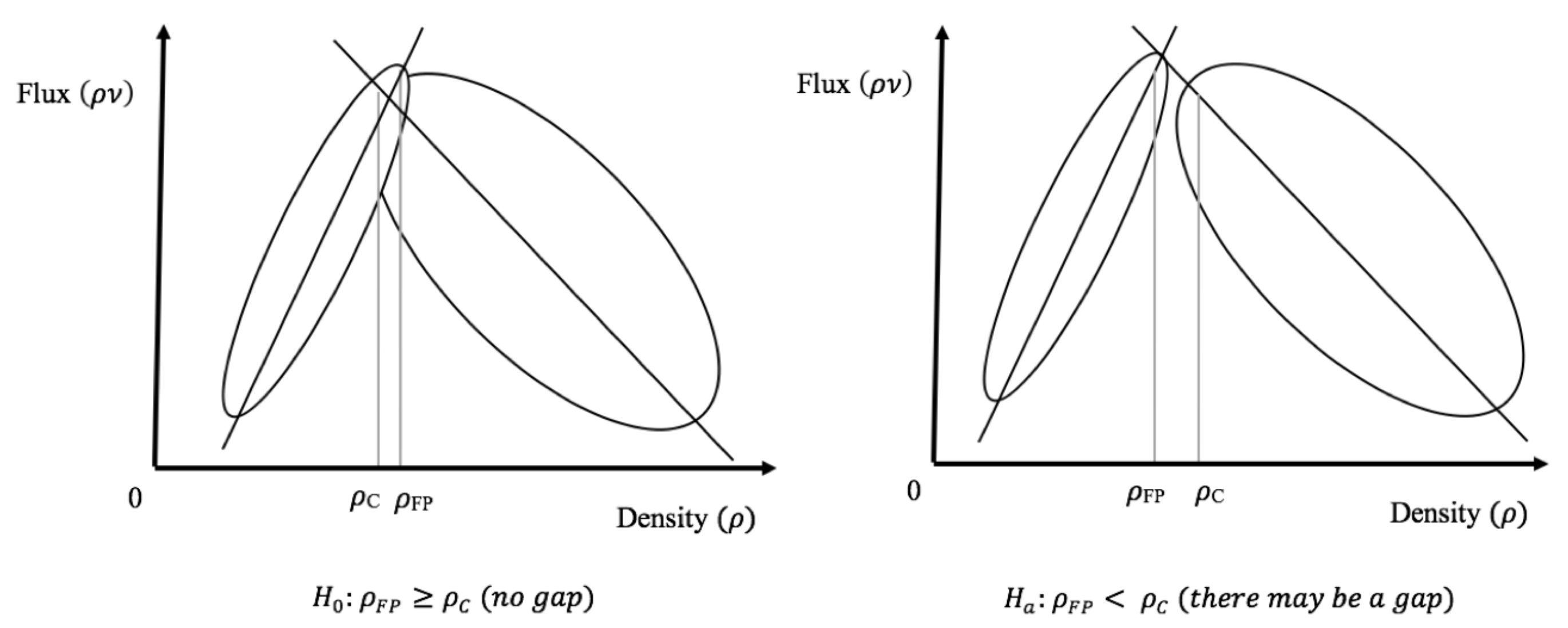
We developed and applied a rigorous hypothesis testing procedure to the datasets to formally investigate the presence of phase transitions. Specifically, investigating the presence of phase transition can be formulated as testing the existence of a “gap region” at the upper portion of occupancy in the free phase and its proximity to the lower portion of occupancy in congestion. As shown in Figure A1 (left) in Appendix A, such gap region can be potentially masked by isolated points in the gap, which could be in fact due to measurement errors or random variations in flux and occupancy. To reduce the impact of these isolated points, we propose to take the upper quantile of the free phase (e.g., 95th percentile, denoted as ) and the lower quantile of the congested phase (e.g., 5th percentile, denoted as ) and formally test for , i.e., there is no gap, against , i.e., there is a gap. Figure 2 illustrates these two scenarios of and .
For given pre-specified percentiles and (e.g., and ), denote and as the corresponding quantiles in the two clusters. The existence of phase transition can be formally tested by a one-sided test based on the Wald statistic
The variance can be approximated by
where and stand for the estimated distribution function and cumulative distribution function of , respectively, and and stand for the number of data points in the free and congestion phases, respectively. The first equality in the calculation of variance is due to the independence of and as they are estimated from different sets of observations. The approximation is due to a standard result for asymptotic variance of percentile estimates (see [19]). The complete sets of results for the statistical analysis on the three datasets can be found in Appendix B.
3. A Macroscopic Second-Order Model Accounting for the 3 Phases
Following the approach of Colombo et al. [7], Fan et al. [14], we propose a new macroscopic model accounting for the three phases derived in the previous sections. In conservation form, the model can be expressed as
where the velocity function is chosen such that
for some , and it is continuous at and . In (1)–(2), the quantity may represent various traffic characteristics, such as vehicles classes [20], aggressiveness [21], desired spacing [22] or perturbation from equilibrium [23], which are transported with the traffic stream. We refer to the variable as a total property [14]. The function v defined in (2) must be:
- Non-negative: for all , ;
- Continuous: and for all
- Vanishing at maximal density: for all
- Non-decreasing with respect to w: for
With the above assumptions, the corresponding flux function satisfies for all w.
To take into account the possible presence of a gap, as suggested by our analysis, we fix the value of the maximal speed in congestion, and let be the density value such that
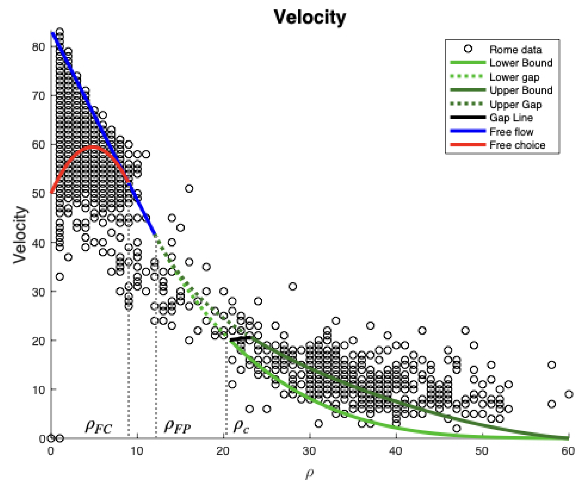
Defining the velocity function (see Figure 3) as
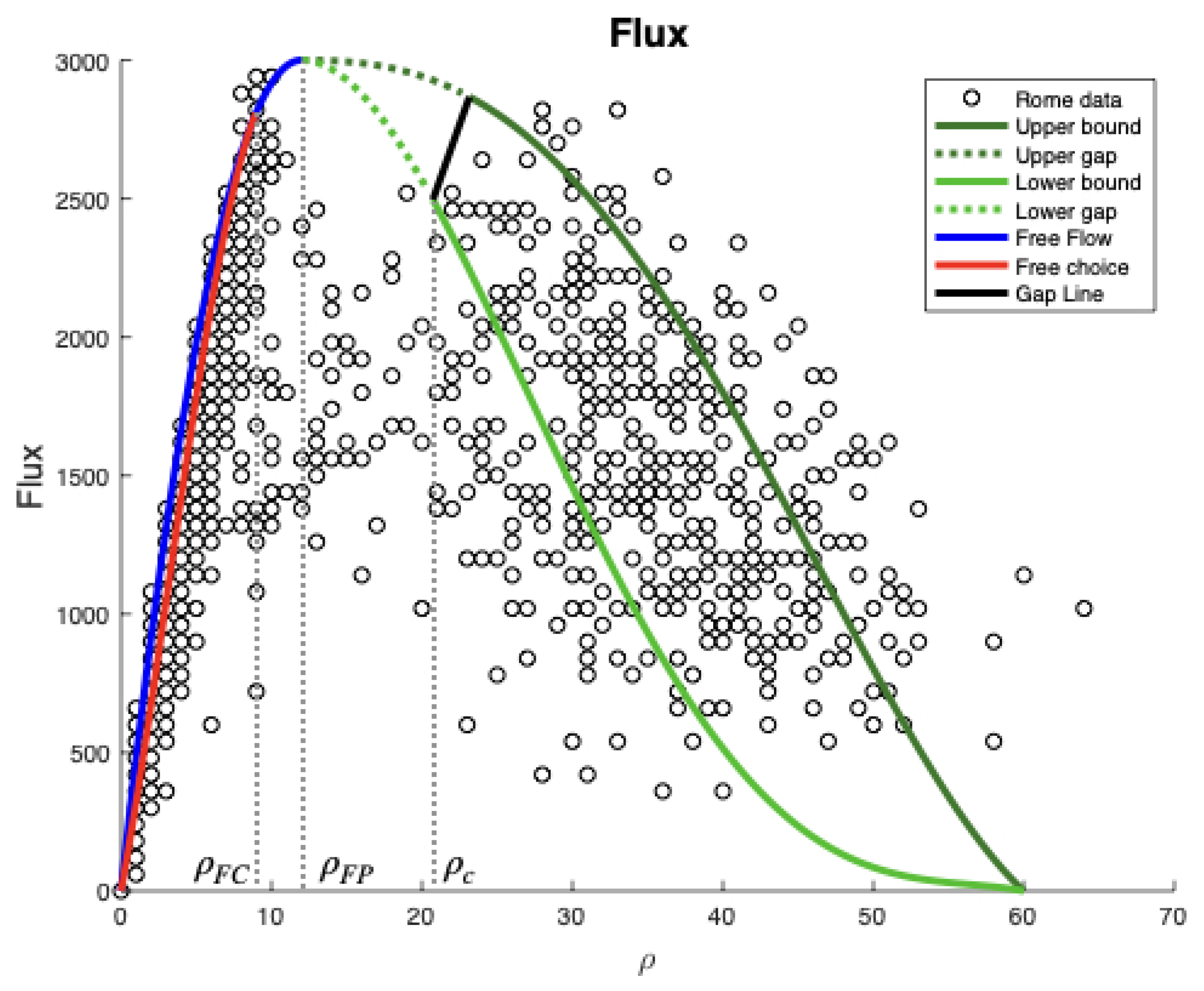
the corresponding flux function displays the desired gap between the free-flow and congested phases (see Figure 4).
3.1. Riemann Solver
To simplify the construction, it is not restrictive to assume that the fundamental diagram is -differentiable, i.e., we assume that
and
System (1) is defined on the invariant domain
We note that, under the above assumptions on the velocity function v, if and only if and . The eigenvalues are given by
so the system is strictly hyperbolic for as long as . We note that the second characteristic field is linearly degenerate, giving origin to contact discontinuity waves, while the first characteristic field is genuinely non-linear if
holds. Moreover, the Riemann invariants of the systems are given by w and v. In particular, the iso-values correspond to waves of the first family (we recall that the system belongs to Temple class, i.e., shock and rarefaction curves coincide) and the contact discontinuities verify . More precisely, in the strictly concave case (5) the elementary waves are constructed as follows.
- 1-rarefaction waves. Two points and are connected by a 1-rarefaction wave if and only if
- 1-shock waves. Two points and are connected by a 1-shock wave if and only ifIn this case, the jump discontinuity moves with speed
- 2-contact discontinuity. Two points and are connected by a 2-contact wave if and only if
In the general (non-concave) case (see Figure 4), the 1-waves consist of a concatenation of shocks and rarefactions (see ([24] Section 1)).
Based on the above elementary waves, the solution corresponding to general Riemann data , can be constructed as follows. Let be the intermediate point defined by
Setting , is given by
In the latter case, a vacuum zone appears between the sector
The complete solution is then given by a 1-wave connecting and , followed by a 2-contact discontinuity between and (eventually separated by a vacuum zone if and ).
The presence of the gap between and does not modify the procedure, since the definition domain
is still invariant. We set with
We can distinguish the following cases:
- If and belongs both to or , the Riemann solver is defined as above.
- If and , the intermediate point belongs to . Let the point defined byThe solution is composed by 1-waves connecting and , a phase-transition jump between and moving with speedfollowed by 1-waves connecting and and eventually a 2-contact from to .
- If and , the intermediate point belongs to . Therefore, the solution always contains a 1-wave (shock phase-transition) from to , followed by a 2-contact discontinuity. Notice that the solution may also contain an intermediate 1-wave in the congested phase.
4. Numerical Scheme and Simulations
4.1. Numerical Scheme
Let us fix constant space step and time step and . Let us define the mesh interfaces for and the intermediate times for . A piecewise constant approximated solution of is given by
In this paper, we use the numerical scheme introduced in [25]. This scheme is a modified Godunov scheme composed of two steps. The first step looks at the evolution in time of the Cauchy problem, while the second step projects it onto piecewise constant functions:
- Step 1: Evolution in time.This step consists in solving the Riemann problem at each cell interface with initial data , obtaining an exact solution .
- Step 2: Projection to timeOnce all Riemann problems at interfaces are solved, Chalons and Goatin [25] proposed a new averaging procedure. The idea is that, since the solution can contain states in different phases, the average is not done on the regular mesh cells but on modified non-uniform cells that contain only values belonging to the same phase. We denote this modified cells by . Afterwards, a sampling strategy allows us to recover a piecewise constant solution on the initial mesh cells .
We define the new interface at time as
and the new space intervals
with the characteristic speeds of propagation of phase transitions at interfaces. Then, we average the solution of Step 1 on the cells , obtaining a piecewise constant approximate solution on a non-uniform mesh with
The modified Godunov scheme then reads:
with
and the solution to the Riemann problem as given in Section 3.1.
We then project the solution onto the original mesh using a well distributed random sequence as follows:
Following Chalons and Goatin [25], we consider the van der Corput random sequence defined by
where , , is the binary expansion of .
4.2. Numerical Simulations
We compared our model (1) to the model in [25] in a simulation on a single road on length 1 with with an initial data
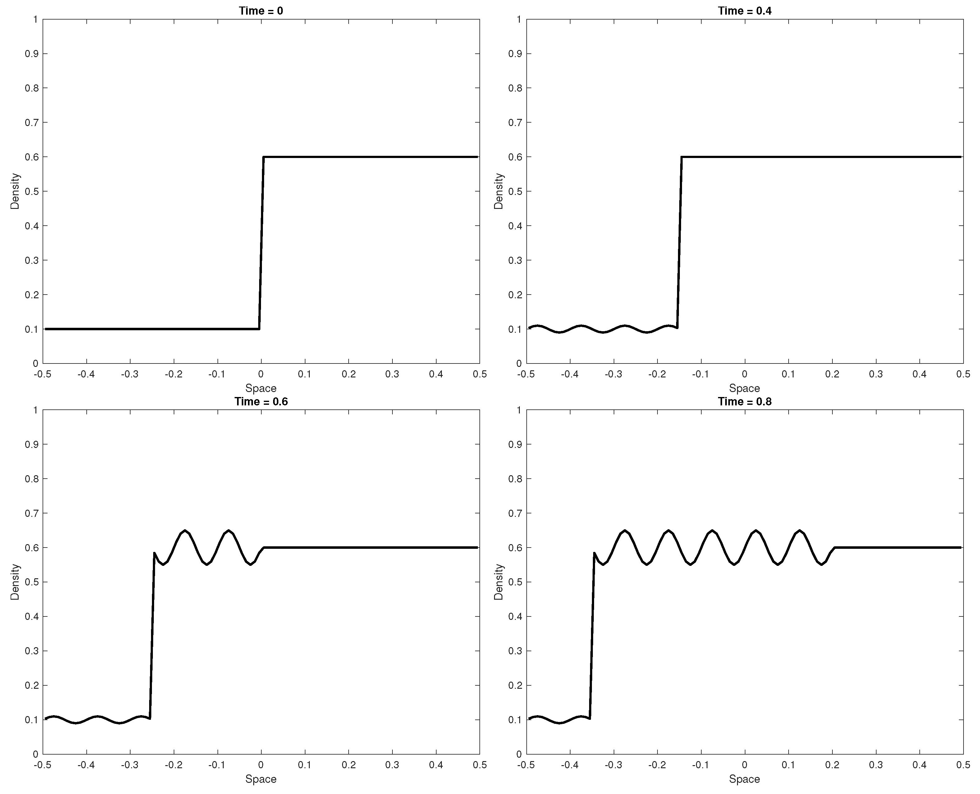
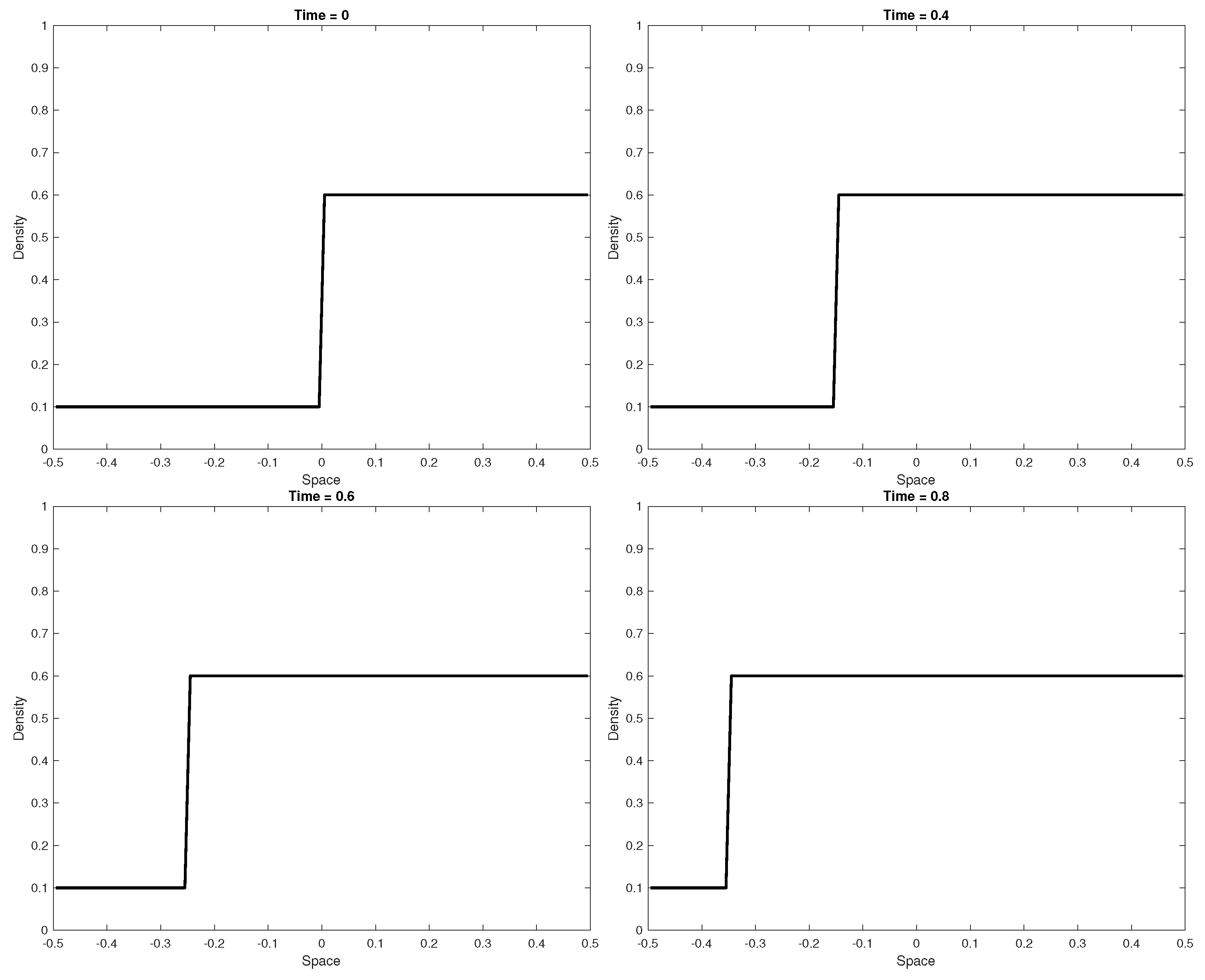
We point out that our model is profoundly different from the phase transition models, even with gap between phases. The main reason is that the second order model (1) admits phase transitions, i.e., shock waves connecting phases, but as classical first family waves, and allows different speeds also in free choice for different values of the variable w. This is well captured by the simulation in Figure 5. An initial condition with one backward moving shock is perturbed by a boundary datum presenting oscillations in the w variable. As a result, for large times, small oscillations are visible on the left (free flow) and large oscillations are propagated through the shock (congested flow). On the other side, the phase transition model of Chalons and Goatin [25] is insensitive to such oscillations in the w variable, as shown in Figure 6.
5. Conclusions
We analyzed three different datasets collected from different locations in Europe and the US from fixed sensors. Representing data via a three-dimensional fundamental diagram, we showed the presence of three traffic phases, two in free flow regime and one in congested flow regime, and of a statistically significant gap between free and congested flow. Based on these results, we designed a new second-order macroscopic model that is capable describing analytically the gap and the three different phases. Moreover, a characterization of Riemann problem solutions and a numerical example are provided, illustrating the difference with phase transition models.
Author Contributions
Software, M.L.D.M. and K.C.; Validation, M.L.D.M.; Visualization, M.L.D.M. and K.H.; Data curation, Y.C. and K.H.; Supervision, Y.C., P.G. and B.P.; Formal analysis, P.G. and B.P.; Methodology, P.G., J.-m.Q. and B.P.; Investigation, J.-m.Q. All authors have read and agreed to the published version of the manuscript.
Funding
Supported by the French National Research Agency under the “Investissements d’avenir” program (ANR-15-IDEX-02). Supported in part by the National Institute of Health grants 1R01LM0126 07 and 1R01AI130460. Supported by the NSF project Grant CNS No. 1446715, the NSF project KI-Net Grant DMS No. 1107444 and the Lopez chair endowment.
Acknowledgments
M.L.D.M. acknowledges that this article was developed in the framework of the Grenoble Alpes Data Institute, supported by the French National Research Agency under the “Investissements d’avenir” program (ANR-15-IDEX-02). Y.C.’s research is supported in part by the National Institute of Health grants 1R01LM012607 and 1R01AI130460. B.P. acknowledges the support of the NSF project Grant CNS No. 1446715, the NSF project KI-Net Grant DMS No. 1107444 and the Lopez chair endowment. The authors thank ATAC S.p.a. for providing the traffic data from the city of Rome and the Départment des Alpes Maritimes for providing data from Sophia Antipolis.
Conflicts of Interest
The authors declare no conflict of interest.
Appendix A. Data Description
Our dataset sources are:
- Rome: Three sensors over one week (June 2006) aggregated every 1 min
- Las Vegas: Fifty sensors over five years (2010–2015) aggregated over every 10 min
- Sophia Antipolis: Four sensors for eight months (January–August 2014) every 6 min
We use the information collected in Rome as the primary example to illustrate the data structure. The Rome dataset contains data of each minute of the entire day for one week; thus, 10,080 observations were collected. Since our primary dataset from Rome consists of one week of observations, we only analyzed data for one week in the other locations as well. The datasets from Las Vegas and Sophia Antipolis were used to validate the results from the Rome data.
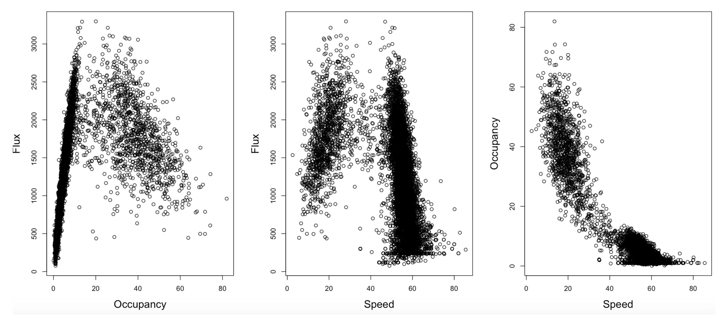
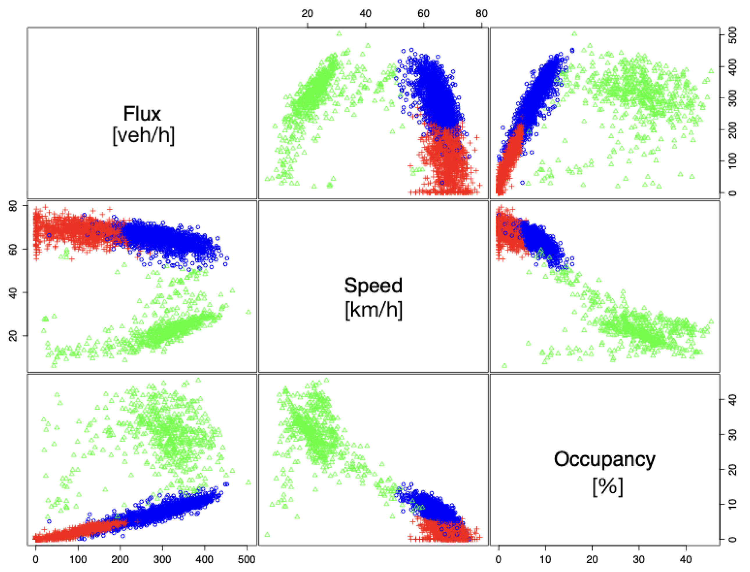
Figure A1 illustrates the pairwise plots among the three measured variables based on the dynamic data collected from a sensor located in the road Viale del Muro Torto in the city of Rome on a Monday. These plots can provide useful insight on the functional relationship between these variables in two-dimensional space. For instance, the plot of flux against occupancy suggests a linear relationship with small variation when occupancy is less than a threshold (known as the free phase) and much larger variation when occupancy is larger than the threshold (known as the congestion phase). Furthermore, both flux vs. speed and flux vs. occupancy plots suggest a possible “gap" between free and congestion phases, which corresponds to phase transition. These are important features that need to be taken into consideration in the mathematical modeling. Such pairwise plots are useful to generate data-driven hypotheses that need to be formally tested statistically and validated across different datasets.
Figure A1.
Pairwise scatterplots of Rome Data in the road Viale del Muro Torto: flux vs. occupancy (left); flux vs. speed (middle); and occupancy vs. speed (right).
Figure A1.
Pairwise scatterplots of Rome Data in the road Viale del Muro Torto: flux vs. occupancy (left); flux vs. speed (middle); and occupancy vs. speed (right).

Appendix B. Results of Cluster Analysis
We conducted model-based cluster analyses on three datasets. We found statistically significant gaps between free and congested phases in all three datasets. We also used regression analysis to demonstrate the existence of free choice phase in explaining the variability in observed flux.
Table A1 presents the results from the described gap analysis of the Rome, Nevada and Sophia datasets. After “trimming” a very small percent of data (e.g., ) and considering quantiles of free and congestion phases, the test statistics suggested strong evidence of a gap (indicating phase transition) in the three datasets.

Table A1.
Results of model-based cluster analysis using Rome, Las Vegas and Sophia Antipolis data. Phase: estimated phase using cluster analysis. FP, free phase; C, congestion phase. Density, estimated density value at the percentile.
Table A1.
Results of model-based cluster analysis using Rome, Las Vegas and Sophia Antipolis data. Phase: estimated phase using cluster analysis. FP, free phase; C, congestion phase. Density, estimated density value at the percentile.
| Dataset | Percentile (%) | Phase | Density | Test Statistic | p-Value |
|---|---|---|---|---|---|
| Rome | 97.5 | FP | 10 | 0 | 1 |
| 2.50 | C | 10 | |||
| 97 | FP | 9 | −1.79 | 0.037 | |
| 3 | C | 10 | |||
| 95 | FP | 9 | −3.15 | <0.001 | |
| 5 | C | 11 | |||
| Las Vegas | 97.5 | FP | 12 | −0.91 | |
| 2.50 | C | 13 | |||
| 97 | FP | 12 | −2.17 | 0.015 | |
| 3 | C | 14 | |||
| 95 | FP | 11 | −5.75 | <0.001 | |
| 5 | C | 16 | |||
| Sophia | 97.5 | FP | 5 | −2.82 | 0.002 |
| 2.50 | C | 10 | |||
| 97 | FP | 5 | −6.44 | <0.001 | |
| 3 | C | 12 | |||
| 95 | FP | 4 | −5.79 | <0.001 | |
| 5 | C | 12 |
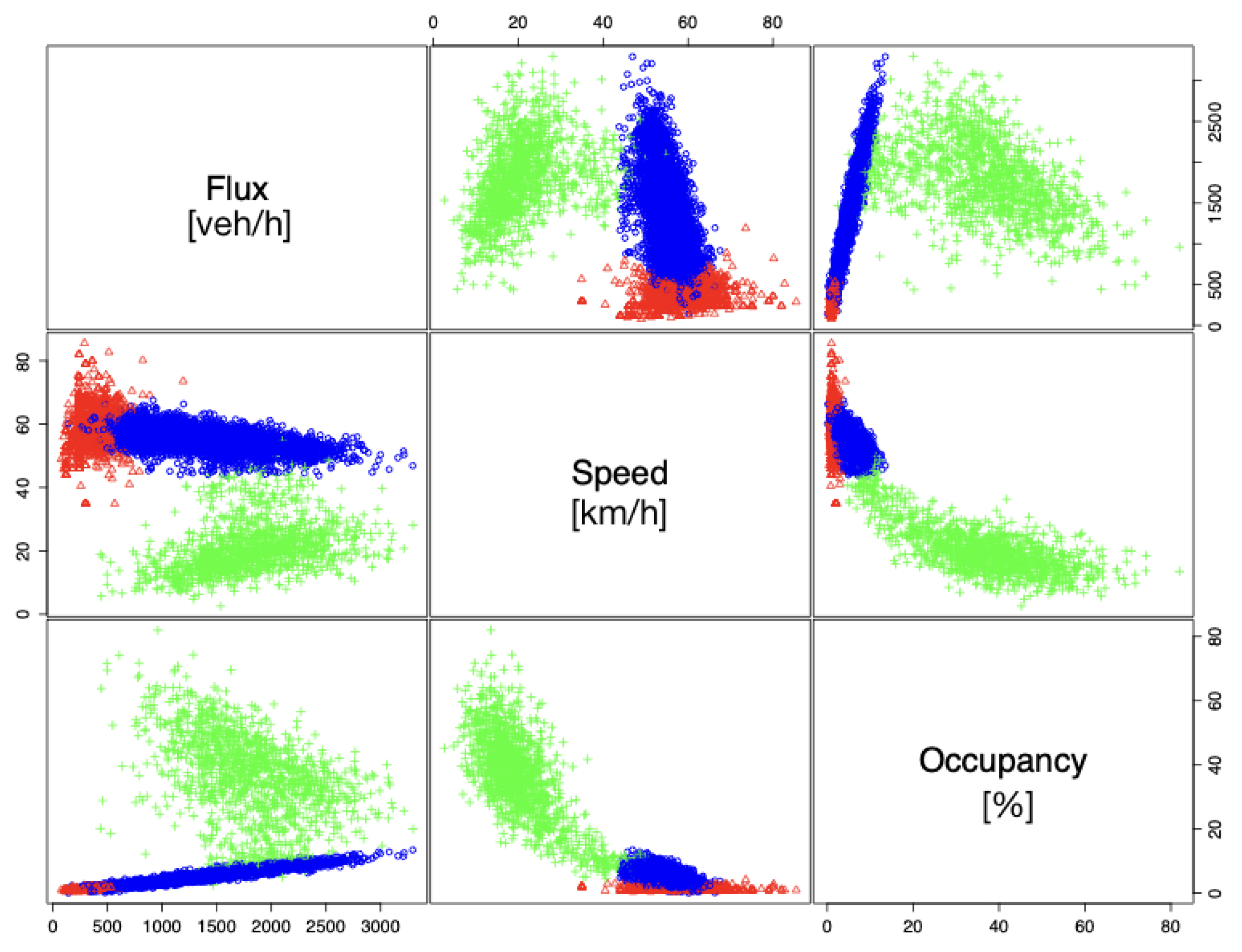
Graphical representations of the results are illustrated below. To clarify the color code for the graphs, the region colored in red corresponds to the Free Choice phase, blue to the Free Flow phase and green to Congestion. The Free Flow phase in this three cluster model corresponds to the remainder of the original conception of Free Flow without Free Choice. The Free Choice and Free Flow phases from the three cluster model are collectively referred to as the Free Phase from here on.
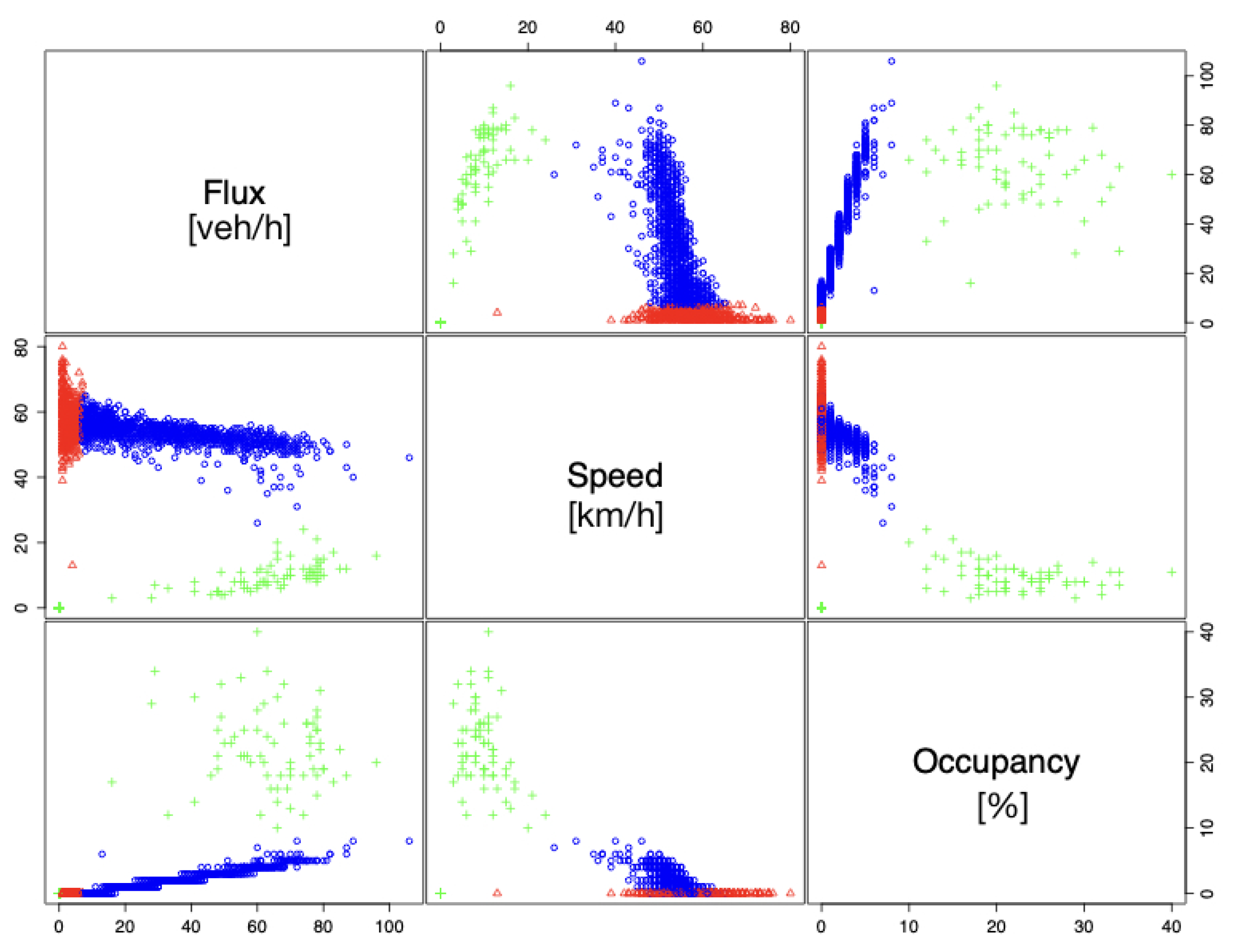
Figure A2 illustrates the clustering performed by ‘mclust’ of the Rome data on a two-dimensional level. Pairs plots present the data according to each pair of variables: velocity and flux, occupancy and flux and velocity and occupancy. This type of plot provides insight on the shape and characteristics of the data in 2D. For instance, we observed some sort of gap between Free Phase and Congestion, which can be most easily viewed in the pairs plot of the variables occupancy and flux. Figure 1 is the three-dimensional representation of the Rome data, a novel approach to visualizing traffic data. Through this 3D plot of data, the proposed gap between Free Phase and Congestion is even more noticeable, reinforcing our observations from the 2D case. Specifying ‘mclust’ to filter through the data for two or three clusters indicated there is some margin of difference between the original Free Flow phase in the two cluster model and the Free Phase in the three cluster model; the latter model is generally neater than the former. The disparity is minimal and perhaps insignificant, although it is worth noting.
Figure A2.
Pairs plot of clustered Rome data.

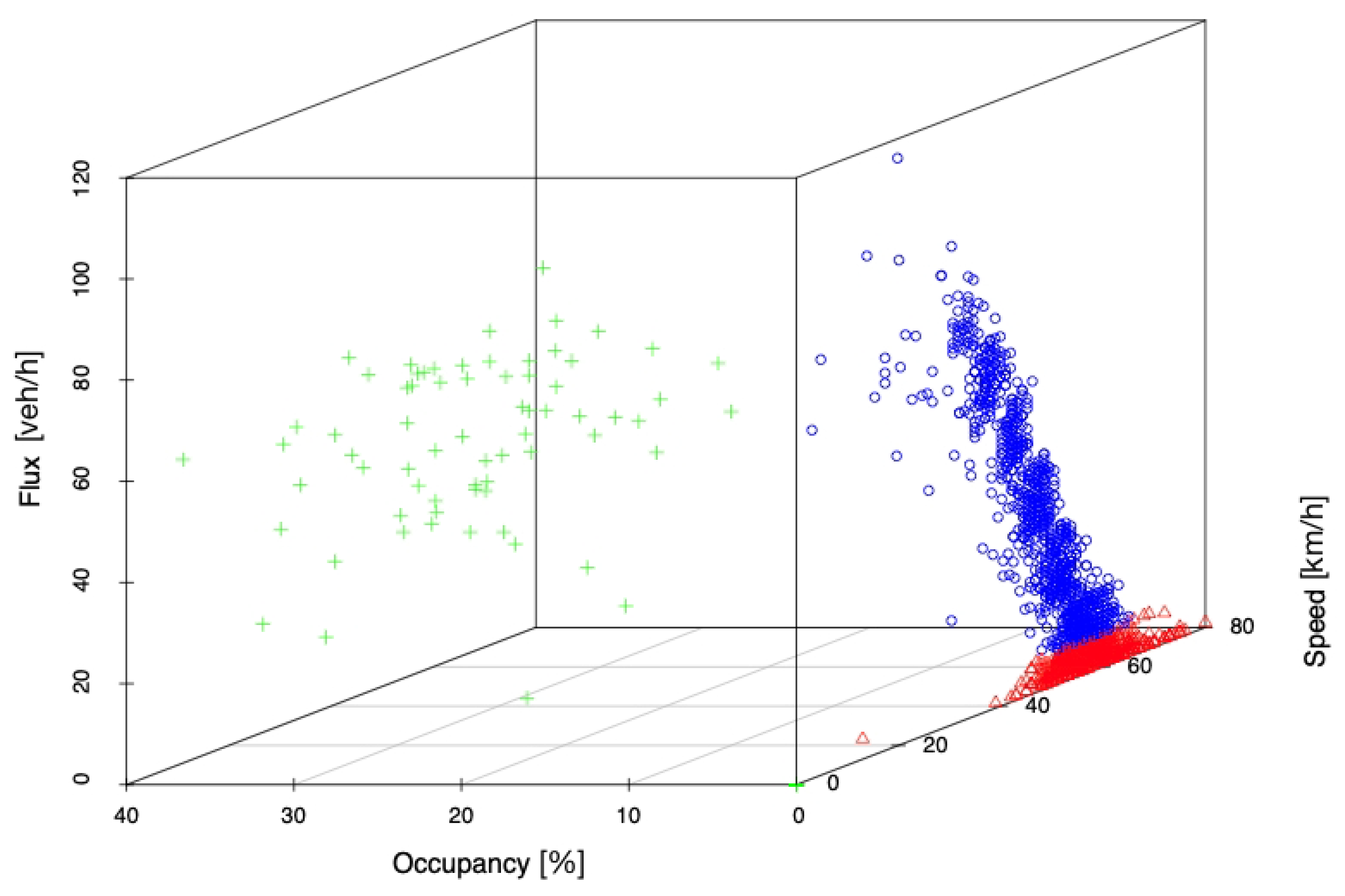
Cluster analyses using the Las Vegas and Sophia Antipolis data corroborate the results obtained with the Rome data. Las Vegas data collected from highway sensors 25 and 99, which we refer to as Nevada 25 and Nevada 99, respectively, clusters into nine phases through ‘mclust’. However, we forced R to choose only two and three clusters to match the original two-phase model of traffic flow proposed by the field and the three-phase model discovered in this study. The results are reported in Figure A3 and Figure A4. The data and analyses suggest that the three-cluster model was preferred using Bayesian information criterion (BIC) for model selection [18].
Figure A3.
Pairs plot of clustered Las Vegas data.

Figure A4.
3D plot of clustered Las Vegas data.

The data from Sophia Antipolis also demonstrate the existence of the Free Choice phase. These two datasets both have a wide range of observed speeds at low levels of occupancy, as shown in the pairs plots and 3D plots in Figure A5 and Figure A6.
Figure A5.
Pairs plot of clustered Sophia Antipolis data.

Figure A6.
3D plot of clustered Sophia Antipolis data.

Appendix Quantifying the Improved Goodness of Fit Through RSS Comparisons
We conducted further analyses by using residual sum of squares (RSS) values to compare various models considered in this paper. The RSS value was calculated as the sum of differences between the observed and fitted values of flux, where the fitted values of flux were obtained from two or three cluster models with or without speed as an additional predictor in addition to the occupancy. The RSS is an objective measure of the remaining variability of the flux that has not been explained by a particular model.
With Rome data, we considered a baseline model with two-phase and occupancy as the only predictor. In other words, this is a 2D and two-phase model as in the existing literature. We calculated the RSS value for this model and compared with the RSS values from more complex models. Specifically, we found that adding speed into the model (i.e., a 3D and two-phase model) explained additionally 1.2% of the variability in observed flux, on top of the baseline 2D and two-phase model. Furthermore, adding the Free Choice phase alone (i.e., a 2D and three-phase model) reduced 13.6% of the remaining variability. Adding both speed and the free choice phase to the model (i.e., a 3D and three-phase model) further reduced 16.0% of the variability in observed flux, compared to the baseline model.
The results of these comparisons suggest that the three-cluster model is indeed superior to the two-cluster model and that 3D rendering of the data is appropriate. The percent change for adjustment of number of clusters as well as dimensions both increases indicates a clear improvement; the three-cluster model is better than the two-cluster model, 3D analysis of data is more informative than that in 2D and the 3D three-cluster model provides the more favorable RSS value overall. These results are consistent across our datasets (see Figure A7, Figure A8, Figure A9 and Figure A10 and Table A2, Table A3, Table A4, Table A5 and Table A6). These results have important implications in understanding traffic flow. They confirm the utility of analyzing this type of data in three dimensions and reveal the presence of a third phase.
Table A2.
RSS analysis with two clusters with flux and occupancy. is the value of the intercept and the occupancy.
Table A2.
RSS analysis with two clusters with flux and occupancy. is the value of the intercept and the occupancy.
| Adj. | RSS | ||||
|---|---|---|---|---|---|
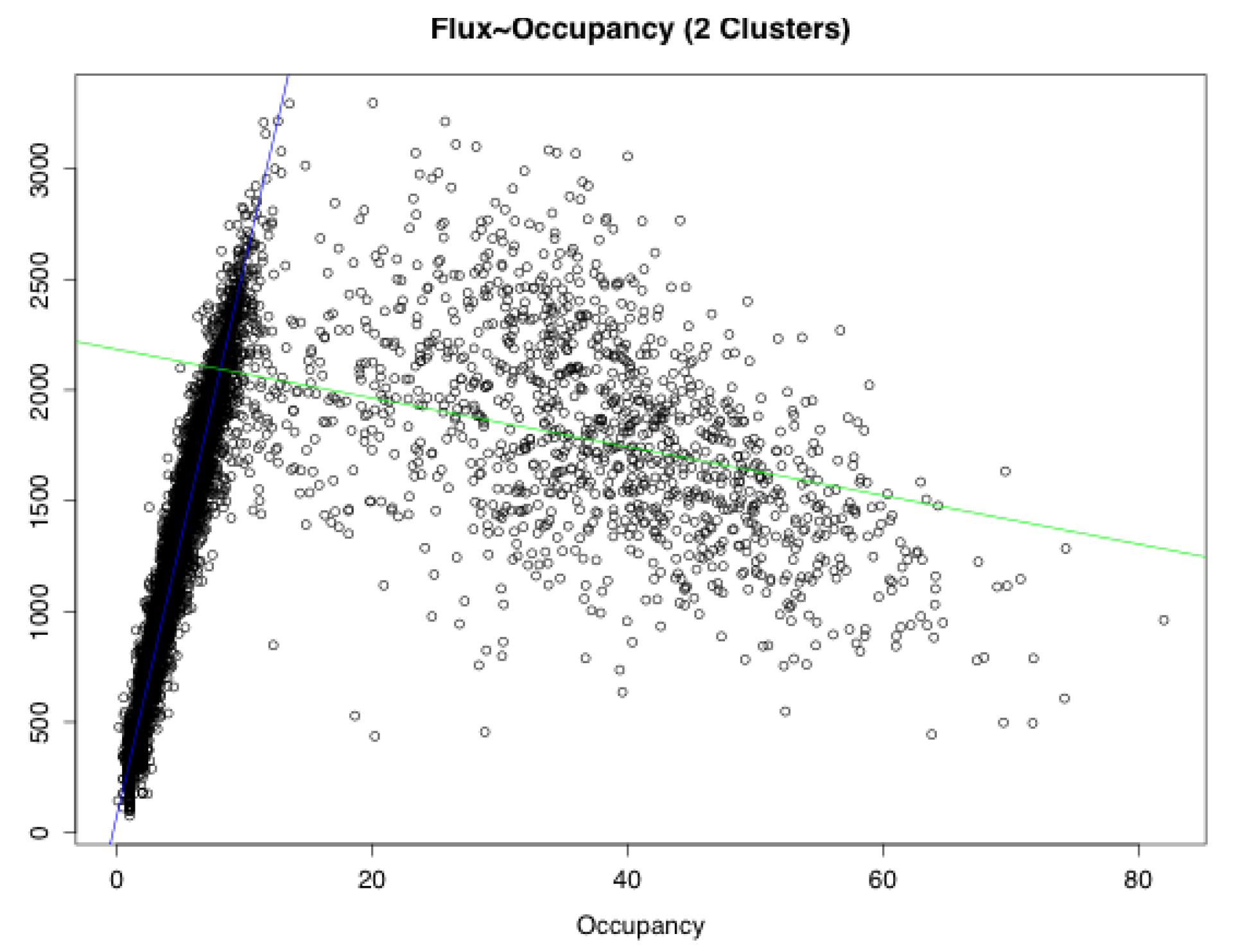
| Free Phase | 77.71 | 249.18 | 0.952 | 0.952 | 157,765,974 |
| Congestion | 2184.09 | −11.00 | 0.09746 | 0.09676 | 283,255,197 |
Figure A7.
Flux vs. occupancy: RSS analysis.

Table A3.
RSS analysis with two clusters with flux, occupancy and speed. is the value of the intercept, the occupancy, and the speed.
Table A3.
RSS analysis with two clusters with flux, occupancy and speed. is the value of the intercept, the occupancy, and the speed.
| Adj. | RSS | |||||
|---|---|---|---|---|---|---|
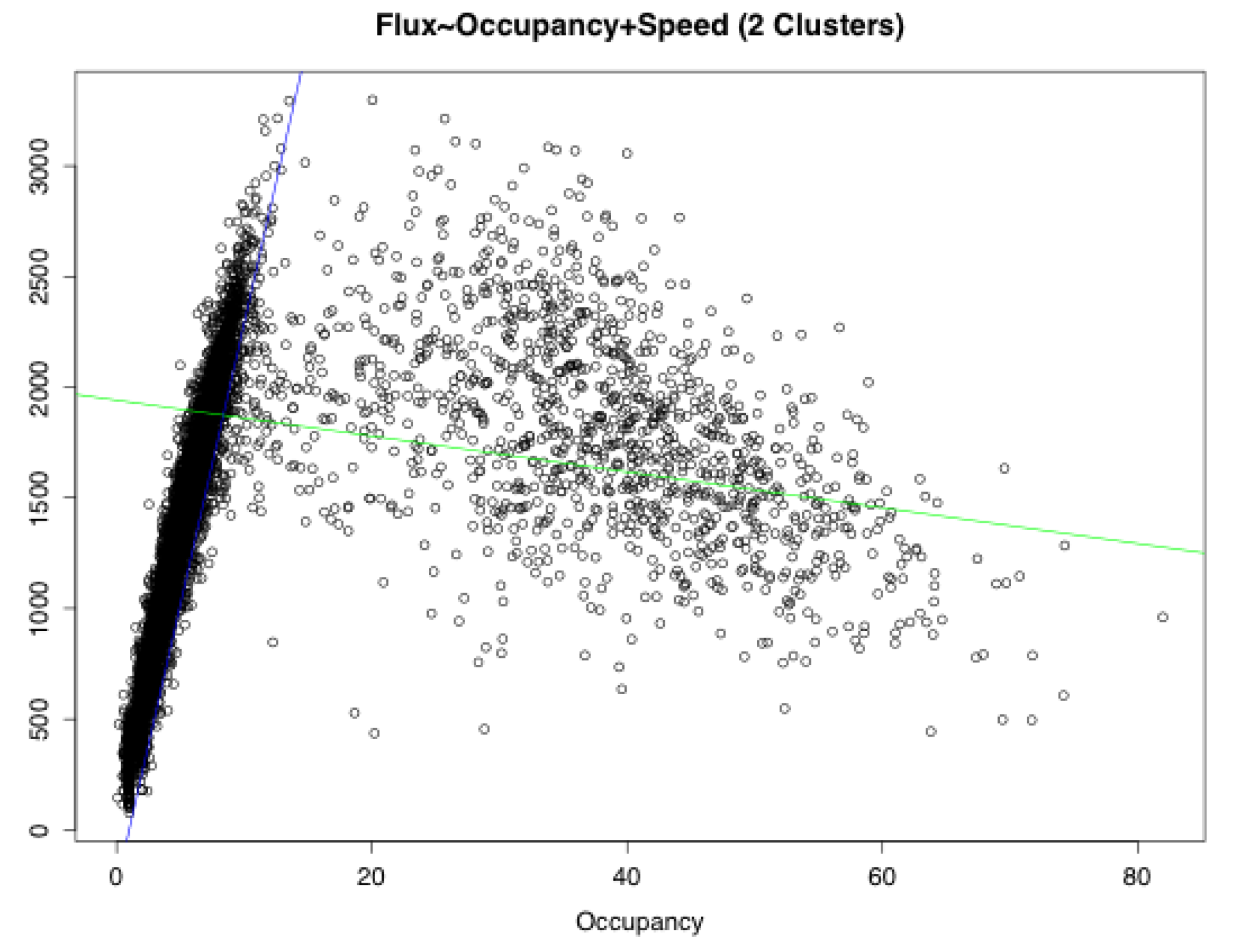
| Free Phase | −248.7 | 253.88 | 5.48 | 0.953 | 0.953 | 154,308,365 |
| Congestion | 1941.54 | −8.11 | 6.64 | 0.1032 | 0.1018 | 281,448,225 |
Figure A8.
Flux vs. occupancy + speed: RSS analysis.

Table A4.
RSS analysis with three clusters with flux and occupancy. is the value of the intercept and the occupancy.
Table A4.
RSS analysis with three clusters with flux and occupancy. is the value of the intercept and the occupancy.
| Adj. | RSS | ||||
|---|---|---|---|---|---|
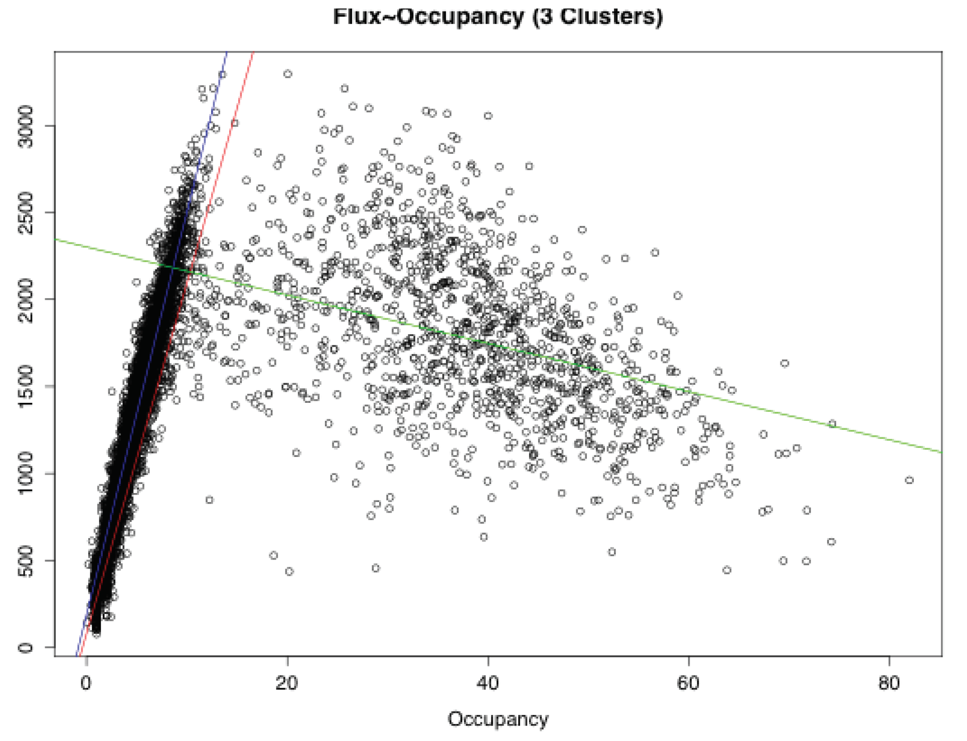
| Free Choice | 79.56 | 201.3 | 0.563 | 0.5628 | 14,269,933 |
| Free Flow | 187.68 | 231.36 | 0.9175 | 0.9175 | 126,714,084 |
| Congestion | 2302.55 | −13.87 | 0.1618 | 0.1611 | 240,324,480 |
Figure A9.
Flux vs. occupancy: RSS analysis.

Table A5.
Residual sum squared analysis with three clusters with flux, occupancy and speed. is the value of the intercept and the occupancy, the speed.
Table A5.
Residual sum squared analysis with three clusters with flux, occupancy and speed. is the value of the intercept and the occupancy, the speed.
| Adj. | RSS | |||||
|---|---|---|---|---|---|---|
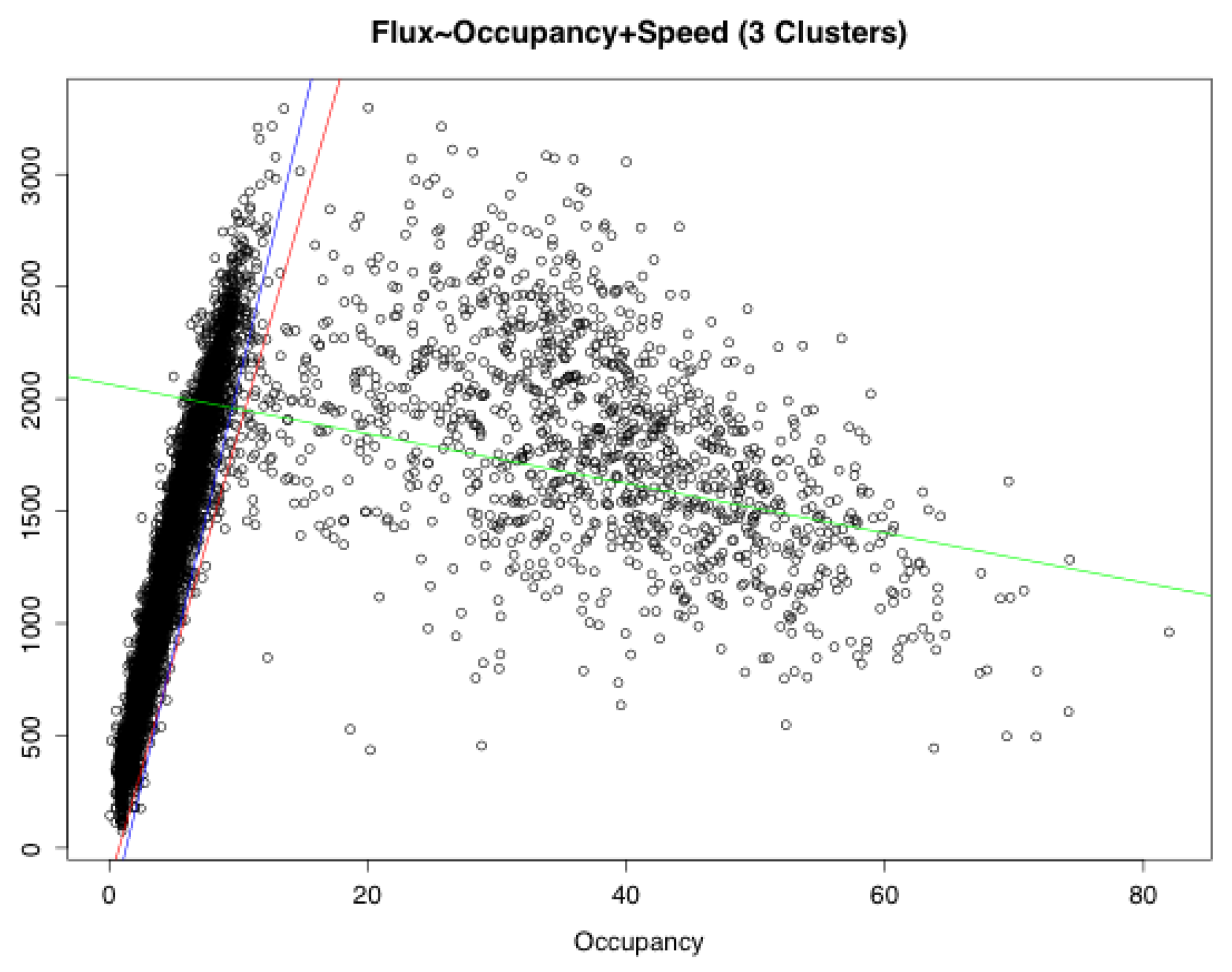
| Free Choice | −153.88 | 200.36 | 4.03 | 0.6033 | 0.603 | 12,951,197 |
| Free Flow | −316.91 | 239.01 | 8.43 | 0.9193 | 0.9192 | 123,984,911 |
| Congestion | 2065.61 | −11.05 | 6.5 | 0.1676 | 0.1663 | 283,641,319 |
Figure A10.
Flux vs. occupancy + speed: RSS analysis.

Table A6.
RSS improvement.
| % RSS Improvement | ||
|---|---|---|
| 2 Clusters | 3 Clusters | |
| 2D | FP: | FC: |
| FF: | ||
| C: | C: | |
| 3D | FP: | FC: - |
| FF: - | ||
| C: | C: - | |
References
- Lighthill, M.J.; Whitham, G.B. On kinematic waves. II. A theory of traffic flow on long crowded roads. Proc. R. Soc. A 1955, 229, 317–346. [Google Scholar]
- Richards, P.I. Shock waves on the highway. Oper. Res. 1956, 4, 42–51. [Google Scholar] [CrossRef]
- Aw, A.; Rascle, M. Resurrection of “second order” models of traffic flow. SIAM J. Appl. Math. 2000, 60, 916–938. [Google Scholar] [CrossRef]
- Zhang, H.M. A non-equilibrium traffic model devoid of gas-like behavior. Transp. Res. Part B Methodol. 2002, 36, 275–290. [Google Scholar] [CrossRef]
- Garavello, M.; Han, K.; Piccoli, B. Models for Vehicular Traffic on Networs; Series on Applied Mathematics; American Institute of Mathematical Sciences: Springfield, MO, USA, 2016; Volume 9. [Google Scholar]
- Colombo, R.M. Hyperbolic phase transitions in traffic flow. SIAM J. Appl. Math. 2003, 63, 708–721. [Google Scholar] [CrossRef]
- Colombo, R.M.; Marcellini, F.; Rascle, M. A 2-phase traffic model based on a speed bound. SIAM J. Appl. Math. 2010, 70, 2652–2666. [Google Scholar] [CrossRef] [Green Version]
- Colombo, R.M.; Goatin, P.; Piccoli, B. Road networks with phase transitions. J. Hyperbolic Differ. Eq. 2010, 7, 85–106. [Google Scholar] [CrossRef] [Green Version]
- Goatin, P. The Aw–Rascle vehicular traffic flow model with phase transitions. Math. Comput. Model. 2006, 44, 287–303. [Google Scholar] [CrossRef]
- Coclite, G.; Garavello, M.; Piccoli, B. Traffic flow on a road network. SIAM J. Math. Anal. 2005, 36, 1862–1886. [Google Scholar] [CrossRef] [Green Version]
- Gerlough, D.L.; Huber, M.J. Traffic Flow Theory; No. HS-006 783; Transportation Research Board: Washington, DC, USA, 1976. [Google Scholar]
- Kerner, B.S. Three-phase traffic theory and highway capacity. Phys. A 2004, 333, 379–440. [Google Scholar] [CrossRef] [Green Version]
- Lebacque, J.P.; Khoshyaran, M.M. A variational formulation for higher order macroscopic traffic flow models of the GSOM family. Transp. Res. Part Methodol. 2013, 57, 245–265. [Google Scholar] [CrossRef]
- Fan, S.; Sun, Y.; Piccoli, B.; Seibold, B.; Work, D.B. A Collapsed Generalized Aw-Rascle-Zhang Model and Its Model Accuracy. arXiv 2017, arXiv:physics.soc-ph/1702.03624. [Google Scholar]
- ATAC, S.p.A. Available online: http://www.atac.roma.it/ (accessed on 3 April 2017).
- Regional Transportation Commission of Southern Nevada (RTC), Freeway and Arterial System of Transportation (FAST) Division. Available online: http://bugatti.nvfast.org/ (accessed on 3 April 2017).
- Département des Alpes Maritimes. Available online: https://www.departement06.fr (accessed on 3 April 2017).
- Fraley, C.; Raftery, A.E. Model-based clustering, discriminant analysis, and density estimation. J. Am. Stat. Assoc. 2002, 97, 611–631. [Google Scholar] [CrossRef]
- Gross, A.J.; Clark, V. Survival Distributions: Reliability Applications in the Biomedical Sciences; John Wiley & Sons: Hoboken, NJ, USA, 1975. [Google Scholar]
- Fan, S.; Work, D.B. A heterogeneous multiclass traffic flow model with creeping. SIAM J. Appl. Math. 2015, 75, 813–835. [Google Scholar] [CrossRef]
- Fan, S.; Herty, M.; Seibold, B. Comparative model accuracy of a data-fitted generalized Aw-Rascle-Zhang model. Netw. Heterog. Media 2014, 9, 239–268. [Google Scholar] [CrossRef]
- Zhang, P.; Wong, S.; Dai, S. A conserved higher-order anisotropic traffic flow model: Description of equilibrium and non-equilibrium flows. Transp. Res. Part B Methodol. 2009, 43, 562–574. [Google Scholar] [CrossRef]
- Blandin, S.; Work, D.; Goatin, P.; Piccoli, B.; Bayen, A. A general phase transition model for vehicular traffic. SIAM J. Appl. Math. 2011, 71, 107–127. [Google Scholar] [CrossRef] [Green Version]
- Bianchini, S. The semigroup generated by a Temple class system with non-convex flux function. Differ. Integral Eq. 2000, 13, 1529–1550. [Google Scholar]
- Chalons, C.; Goatin, P. Godunov scheme and sampling technique for computing phase transitions in traffic flow modeling. Interfaces Free Boundaries 2008, 10, 197–221. [Google Scholar] [CrossRef] [Green Version]
Figure 1.
3D visualization and cluster analysis results of Rome data suggest the existence of third phase (red) in addition to the free flow (blue) and congestion (green) phases.
Figure 1.
3D visualization and cluster analysis results of Rome data suggest the existence of third phase (red) in addition to the free flow (blue) and congestion (green) phases.

Figure 2.
Illustration of hypothesis testing procedure for phase transition.

Figure 3.
An example of speed function.

Figure 4.
General (non-concave) fundamental diagram.

Figure 5.
Evolution of the density for our model on a single road.

Figure 6.
Evolution of the density for a classical phase transition model on a single road.

Publisher’s Note: MDPI stays neutral with regard to jurisdictional claims in published maps and institutional affiliations. |
© 2021 by the authors. Licensee MDPI, Basel, Switzerland. This article is an open access article distributed under the terms and conditions of the Creative Commons Attribution (CC BY) license (http://creativecommons.org/licenses/by/4.0/).
Share and Cite
MDPI and ACS Style
Delle Monache, M.L.; Chi, K.; Chen, Y.; Goatin, P.; Han, K.; Qiu, J.-m.; Piccoli, B. A Three-Phase Fundamental Diagram from Three-Dimensional Traffic Data. Axioms 2021, 10, 17. https://doi.org/10.3390/axioms10010017
AMA Style
Delle Monache ML, Chi K, Chen Y, Goatin P, Han K, Qiu J-m, Piccoli B. A Three-Phase Fundamental Diagram from Three-Dimensional Traffic Data. Axioms. 2021; 10(1):17. https://doi.org/10.3390/axioms10010017
Chicago/Turabian StyleDelle Monache, Maria Laura, Karen Chi, Yong Chen, Paola Goatin, Ke Han, Jing-mei Qiu, and Benedetto Piccoli. 2021. "A Three-Phase Fundamental Diagram from Three-Dimensional Traffic Data" Axioms 10, no. 1: 17. https://doi.org/10.3390/axioms10010017
Note that from the first issue of 2016, this journal uses article numbers instead of page numbers. See further details here.