Cloud Detection from Radio Occultation Measurements in Tropical Cyclones

Abstract

Tropical cyclones (TC) are one of the main producers of clouds in the tropics and subtropics. Hence, most of the clouds in TCs are dense, with large water and ice content, and provide conditions conducive to investigate clouds’ impact on Radio Occultation (RO) measurements. Although the RO technique is considered insensitive to clouds, recent studies show a refractivity positive bias in cloudy conditions. In this study, we analyzed the RO bending angle sensitivity to cloud content during tropical cyclone seasons between 2007 and 2010. Thermodynamic parameters were obtained from the ERA-Interim reanalysis, whereas the water and ice cloud contents were retrieved from the CloudSat profiles. Our experiments confirm the positive mean RO refractivity bias in cloudy conditions that reach up to more than 0.5% at the geometric height of around 7 km. A similar bias but larger and shifted up is visible in bending angle anomaly (1.6%). Our results reveal that the influence of clouds is significant and can exceed the RO bending angle standard deviation for 21 out of 50 (42%) investigated profiles. Mean clouds’ impact is detectable between 9.0 and 10.5 km, while, in the case of single events, clouds in most of the observations are significant between 8 and 14 km. Almost 15% of the detectable clouds reach 16 km height, while the influence of the clouds below 5 km is insignificant. For more than half of the significant cases, the detection range is less than 3 km but for one observation this range spreads to 7–8 km.

1. Introduction

GPS Radio Occultation (RO) is an active limb viewing technique that takes advantage of phase and amplitude of two L-band electromagnetic signals transmitted from GPS and received on low earth orbit (LEO) satellites [1]. A GPS signal passing through Earth’s atmosphere is refracted and attenuated, which induces delay and bending. A measure of the atmospheric density in terms of the bending angle parameter is derived from Doppler shifts based on precise clocks, satellite orbits and velocity measurements. Since the GPS signal is considered to be insensitive to clouds, it can be used in any weather condition [2] and enables observations with high accuracy, precision and vertical resolution [1]. However, as in any observations, RO measurements are affected by noise, which is attributed to three main sources: instrumental, ionospheric and small-scale turbulence [3]. The profiles of the neutral atmosphere retrieved from RO observations are the most accurate within the upper troposphere and lower stratosphere. Scherllin-Pirscher et al. [4] demonstrated that the global mean observation errors are as low as 0.3% for bending angle, 0.1% for refractivity and 0.2 K for a dry temperature at altitudes between 4 and 35 km.

The difference between dry RO parameters and actual parameters is negligible above about 8–12 km altitude [4]. In dry retrievals where the temperature is low enough (i.e., T < 250 K) [5], water vapor is neglected and ideal gas and equilibrium assumptions can be applied. Next, atmospheric pressure and accurate temperature profiles can be derived using reduced refractivity equation. In wet retrievals, the dry assumption is invalid and water vapor influence cannot be neglected. In this case, additional information about temperature, pressure or water vapor pressure is needed to retrieve the physical atmospheric parameters. In general, a priori information from global weather analysis is combined with RO profiles in one-dimensional variational (1DVar) method.

RO profiles contain valuable information about the atmosphere around the tropopause and they are useful in the investigation of deep convective storms and tropical cyclones [6,7,8]. Tropical cyclones (TC) are destructive natural hazards, which affect wide tropical and subtropical areas and cause catastrophic damage including consequences to public health [9] and strong socioeconomic impact [10]. TCs are very dangerous not only because they produce strong winds, copious rainfall and wind-driven waves but also because of the storm surges that can result in floods and landslides [11]. Maximum mean wind speed is a key parameter defining the intensity of TC. This speed is usually estimated applying Dvorak technique to visible and infrared satellite images [12], or rarely using in situ measurements. Furthermore, Vergados et al. [13] demonstrated a new way of estimating TC intensity based on temperature profiles from RO observations.

Remote sensing observations of cloud-top height, cloud-top temperature and cloud profiling information are an important input to the TC strength prediction [14]. In mature TC, the eye of the storm is dominated by outward sloped low-level clouds such as stratus or convective stratocumulus clouds, while TC outflow consists of upper-level cirrus and cirrostratus [15]. In general, a fraction of very cold clouds within TC is much higher compared to clouds outside TC and such clouds contribute to the local cooling of the cold-point tropopause by 10 K. Furthermore, 29% of the clouds reach a temperature of 15 K below the temperature of the tropopause and 9% of them penetrate the tropopause [16]. In the tropics, the change from the troposphere to the stratosphere occurs gradually in a layer rather than at a sharp tropopause. This layer is called the tropical tropopause layer (TTL) and is defined with a bottom at 14 km and a top at 18.5 km. Convective clouds in TTL reach altitudes around 10–15 km or even higher, overshooting the TTL [17]. Tropopause and TTL can be accurately determined using RO measurements which are very sensitive to the vertical temperature gradients. Furthermore, this ability allows comprehensive investigating TC thermal structure with cold anomaly and TC overshooting of the tropopause [18,19].

Due to its all-weather, all-day capabilities, the RO technique could be useful in TC cloud detection. Lin et al. [20], as one of the first, analyzed RO refractivity and temperature profiles in cloudy and clear conditions and identified impact of clouds to RO retrieval based on collocated CloudSat observations. They found positive refractivity bias of differences between RO and National Centers for Environmental Prediction–National Center for Atmospheric Research (NCEP-NCAR) reanalysis and European Centre for Mediu—Range Weather Forecasts (ECMWF) analysis in cloudy-sky, while, in contrast, the negative bias was observed in clear areas. Furthermore, the mean temperatures differences between models and RO near and just below the cloud top demonstrate positive anomaly with a maximum around 1–2 K. However, this analysis was limited to clouds with top below 12 km to avoid the compounded effect of the tropopause.

Yang and Zou [21] and Zou et al. [22] extended the work of Lin et al. [20] by evaluating the contribution of liquid water content (LWC) and ice water content (IWC) of clouds to RO refractivity using CloudSat data. The impact of LWC on total refractivity reaches 0.8% by single clouds. At the same time, IWC contribution to the total refractivity increases linearly with the amount of IWC and reaches a maximum of about 0.6% at 1 g m${}^{-3}$. Thus, it was proposed to include the clouds’ effect in RO retrievals because a 1% uncertainty in refractivity could introduce significant errors in derived water vapor profiles. Furthermore, Hordyniec [23] reported that neglect the clouds with the contribution of 0.7% to the total value in terms of refractivity introduce bending error of nearly 4%.

RO-based cloud studies on the impact of the IWC and LWC [20,21,22] were based on thorough experimental studies but did not use the RO uncertainty to investigate the significance of this impact. Furthermore, previous clouds’ impact studies on the RO signal were focused on refractivity, which is a product that requires spherical symmetry assumption to be calculated. Thus, for the first time, we investigated an impact of clouds on RO bending angle retrieval using ice and liquid refractivities, as well as bending angle uncertainties.

The aim of this work was to examine how sensitive RO observations are to the presence of clouds in TCs during 2007–2010. Dense clouds, i.e. the anvils, cumulus, and cumulonimbus clouds associated with TCs, provide an excellent environment to study clouds’ impact on GNSS signal. Based on the assumption of spherical symmetry, ERA-Interim refractivity profiles were converted to the bending angle, including and excluding cloud effect derived from CloudSat measurements, and validated against RO error retrievals. In the final step, we investigated the extent of the atmosphere where clouds are detectable, the frequency of selected observations and bias magnitude.

This paper is organized as follows. The datasets used in this study are described in Section 2. The theoretical background of clouds’ impact on RO retrievals and our methodology are provided in Section 3. Section 4 presents numerical results on estimating RO sensitivity to the presence of clouds in TC. Discussion, our conclusions and future work are provided in Section 5 and Section 6.

2. Data

2.1. RO Profiles

In our research, we focused on RO optimized bending angle, bending angle standard deviations and refractivity profiles between altitudes of 2 and 20 km during tropical cyclones. We analyzed GPS RO profiles from the Constellation Observing System for Meteorology, Ionosphere and Climate (COSMIC). The data for this mission are available on the COSMIC Data Analysis and Archive Center (CDAAC) website. We considered Atmospheric Profile (atmPrf) and Wet Profiles (wetPrf) data from 2007 to 2010 during tropical cyclone seasons when CloudSat data are fully available.

RO-based profiles (atmPrf files) are stored in NetCDF format and contain bending angle, bending angle uncertainty, impact parameter, dry pressure and temperature. All data are provided against geometric height above mean sea level. The same meteorological parameters contained in wetPrf are based on a 1DVar technique adapting European Center for Medium-Range Weather Forecast (ECMWF) analysis as a first guess.

The geometry optics approximation of interfering rays is able to derive the bending angle from an instantaneous frequency above the troposphere as single tone signals. However, the residual noise induced by L2 frequency in the ionospheric calibration amplifies the uncertainty of the retrieved bending angle. The root mean squared error of fluctuations in the LC Doppler within 1 s sliding window is used to estimate the standard deviation of the bending angle in the stratosphere [24].

Bending angle standard deviation (${\sigma }_{ba}$) is one of the key parameters that were applied in this study. In the RO technique, the measured wavefield is mapped into the representation of the unique impact parameter for each ray assuming a spherically-symmetric medium. However, in the lower troposphere, the presence of horizontal gradients induces the variation of the impact parameter along a ray-path and the bending angle profile can become multivalued [3].

In the presence of multipath effects, single rays can be disentangled with the applications of Fourier integral operators [25]. The bending angle is calculated from the raw complex signal, yielding a sub-Fresnel resolution. The running spectra of transformed L1 and L2 wavefields in the time domain allow assessing observational errors of the bending angle in the troposphere ${\sigma }_{ba}$ [3]. This will result in larger bending error for regions with non-uniqueness of ray propagation. This approach is operationally used in the CDAAC processing to assign uncertainties to the bending angle [26].

2.2. Global Atmospheric Reanalysis

ERA-Interim (ERA) is a global atmospheric reanalysis that is produced by the ECMWF [27]. The retrieved dataset contains meteorological parameters, such as temperature, pressure and specific humidity for 37 vertical pressure layers with a resolution of 25 hPa between 1000 and 750 hPa, 50 hPa below 250 hPa layer and 16 irregularly spaced levels above. The ERA data assimilation system adopts a four-dimensional variational analysis with a 12-h analysis window and provides products four times a day with a horizontal resolution of approximately 80 km between grid points. The background profiles of pressure, temperature and water vapor at RO locations generated from global reanalysis fields are provided in CDAAC eraPrf product [28]. The quality of ERA-Interim reanalysis is improved compared to preceding ERA-40 reanalysis. The ECMWF product is consistent with the verifying soundings for temperature; however, a cold bias of more than 1 K at upper levels is still observed. At the same time, relative humidity below 250 hPa differs greatly from the validation set by 10–12% [29].

2.3. Remote Sensing of Cloud Water Content

The CloudSat mission was launched on 28 April 2006, in sun-synchronous near-polar orbit at approximately 705 km above the earth’s surface. This mission provides a global view of the vertical structure of aerosols and clouds. The mission was fully operated until April 2011 when the satellite experienced a battery anomaly. The Cloud Profiling Radar (CPR), an instrument on board CloudSat satellite, is a 94-GHz nadir-looking radar that measures the power backscattered by hydrometeors as a function of the distance from the radar with a minimum sensitivity of −30 dBZ. Each vertical profile is acquired for an integration time interval of 0.16 s, which corresponds to cross track horizontal resolution of 1.4 km and 1.8 km along the track. CPR provides 125 samples per profile with the effective vertical resolution of 240 m covering troposphere inside the 30 km data window [30]. The liquid and ice water cloud contents assessed by 2B-CWC-RO data product version R04 are used in this study to evaluate clouds effect on bending angle retrievals. CloudSat is in close agreement with other sensors but IWC retrieval error is less than 50% within overlapping sensitivity range [31]. We focused on cloud profiles released by CloudSat in the period 2007–2010 within the radii of tropical cyclones and coincided with the RO events.

2.4. TC Tracks

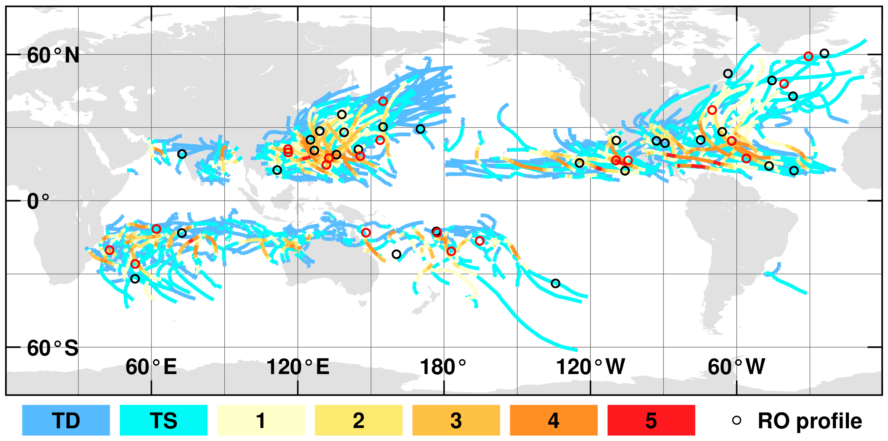
In this research, we considered tropical cyclone seasons during 2007–2010. We downloaded detailed information about TC tracks from The International Best Track Archive for Climate Stewardship (IBTrACS) (illustrated in Figure 1). IBTrACS contains merged information about TCs with global coverage from many of the WMO-recognized Regional Specialized Meteorological Centers (RSMC), which officially forecast and monitor tropical cyclones in their region of responsibility [32]. The data are stored in NetCDF or plain text format and consist of information about name, dates of occurrence, coordinates, intensity and minimum pressure at least every 6 h. Additionally, for western North Pacific and the South China Sea, direction and radii of 30 knot wind were retrieved.

Best-track data are products from postseason reanalysis of a storm’s position and intensity from all available data sources, such as satellite, surface and ship observations, which vary depending on the agency. Combining data from all RSMC raises numerous issues. For example, because every storm can be monitored by many agencies, each storm must be identified uniquely, all errors in time and longitude (e.g., wrong sign when crossing timeline or one-day time offset) need to be eliminated, and estimated storm intensities need to be merged into one. The wind speed measurements are not consistent across RSMCs because the agencies use different averaging periods of maximum sustained wind speed, i.e., 1-, 2-, 3-, and 10-min. Hence, the data must be transformed to the consistent averaging period using conversion factors, which adds to the overall uncertainty of IBTrACS [32]. In this study, we used the factor 1.14 to convert 10-min to 1-min wind speeds [33].

3. Methods

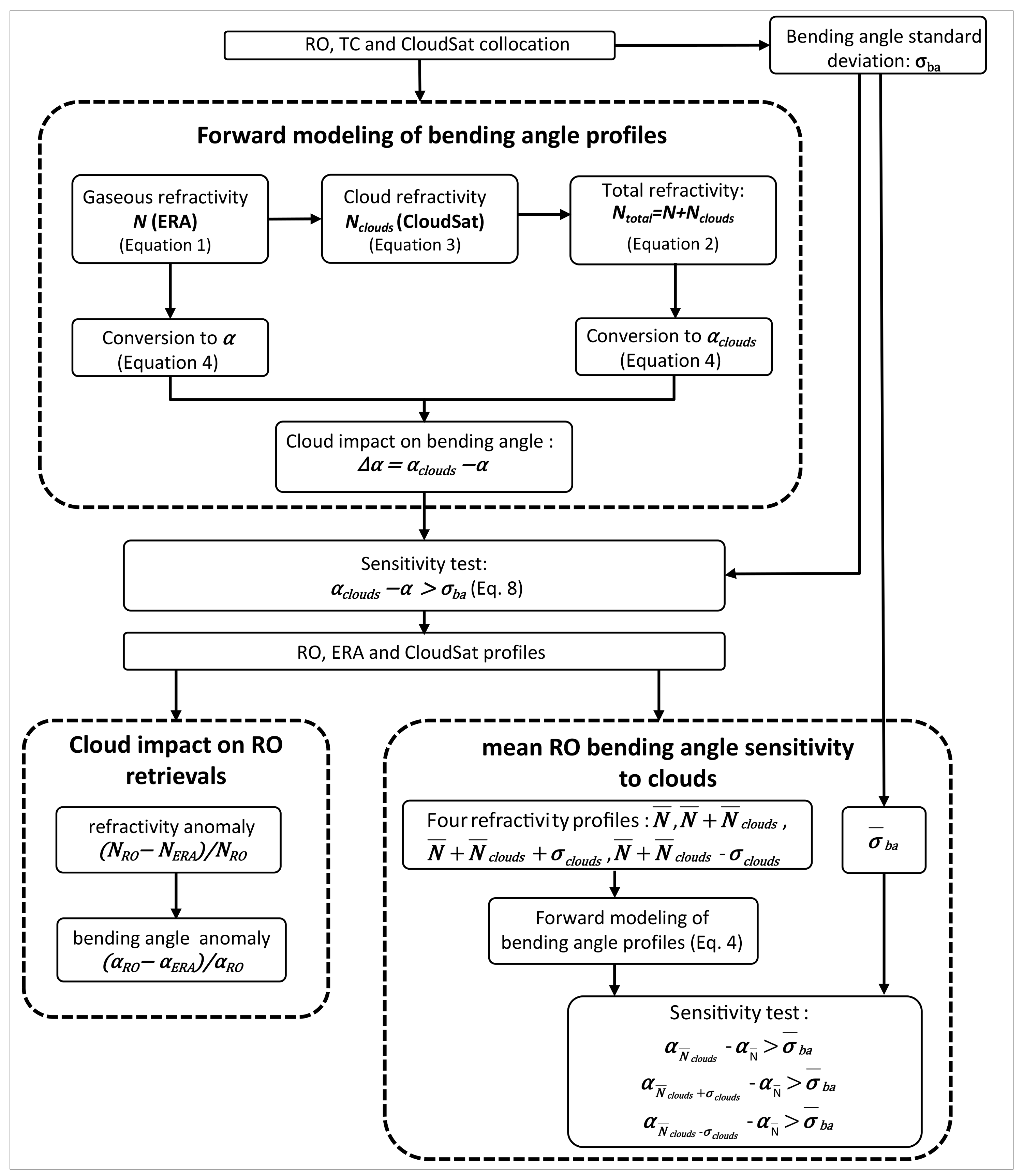
Our study was divided into three main steps:

• Using meteorological parameters provided in eraPrf products and additional collocated CloudSat measurements, refractivity profiles with and without clouds were calculated. The obtained profiles were converted to bending angles, and potential clouds’ impact on bending angle was assessed as the difference between them. Cloud content is significant if the computed difference exceeds bending angle standard deviation.
• Clouds’ impact on RO refractivity and bending angle were estimated as fractional differences between RO observations and ERA background.
• RO sensitivity to the presence of clouds was investigated. Based on cases with significant cloud content, we calculated four kinds of refractivity profiles: mean gaseous, mean gaseous plus mean cloud, mean gaseous plus mean cloud plus standard deviation of clouds and mean gaseous plus mean cloud minus standard deviation. We then tested whether assessed clouds impacts on bending angle are significant and exceed mean observation error provided by the CDAAC in atmPrf.

A brief summary of the entire process described above is illustrated in Figure 2 and presented in detail in the following sections.

3.1. Forward Modeling of Bending Angle Profiles

Both gaseous and non-gaseous components can refract the GPS signal as it passes through the atmosphere. The atmospheric refractive index (n) is defined as the ratio between the speed of light in a vacuum and corresponding medium of propagation. Since the refractive index in a neutral atmosphere is almost equal to unity, it is convenient to express it in terms of the refractivity: $N=(n-1)·{10}^{-6}$. Usually, refractivity is considered to be proportional to temperature (T), pressure (P) and water vapor (e), as described by Smith and Weintraub [34]:

$$N=77.6\frac{P}{T}+3.73·{10}^5\frac{e}{T^2}.$$

(1)

However, the non-gaseous refractivity, containing the contribution of liquid and ice water could also be taken into account. Clouds contribute to the total refractivity according to equation:

$$N_{total}=N+N_{clouds},$$

(2)

where $N_{clouds}$ is defined as:

$$N_{clouds}=N_{lw}+N_{ice}\approx 1.45LWC+0.69IWC,$$

(3)

and $N_{lw}$ and $N_{ice}$ are liquid water and ice induced, refractivity.

The meteorological parameters mentioned in Equation (1) can be retrieved from eraPrf products but $LWC$ and $IWC$ (Equation (3)) must be assessed from collocated CloudSat profiles.

Total refractivity can be simulated in two ways: first, using gaseous part only (Equation (1)); or, second, including cloud water (Equation (2)). Next, the derived refractivities can be converted to bending angles, taking into account that the most significant change in bending angle is attributed to vertical density gradients [5]. Therefore, the spherical symmetry of the refractive index field is assumed and the total refractive bending angle ($\alpha$) can be expressed as:

$$\alpha \left(a\right)=2{\int }_{r_t}^{\infty }d\alpha =2a{\int }_{r_t}^{\infty }\frac{1}{\sqrt{n^2{r}^2-a^2}}\frac{dln\left(n\right)}{dr}dr,$$

(4)

where r is distance from the center of curvature of a ray path and the integral is over the portion of the atmosphere above the radius of the tangent point $r_t$ and impact parameter a, which is constant for a given ray path. In a spherically symmetric atmosphere, the impact parameter can be derived from Bouguer’s rule as: $a=rnsin\left(\theta \right)$, where $\theta$ is the angle between the position vector and the tangent of the ray path.

The two datasets—(1) bending angles $\alpha$, using traditional gaseous atmosphere refractivity Equation (1); and (2) bending angles using refractivities including cloud effects ${\alpha }_{cloud}$ in Equation (2)—were used to assess the potential impact of clouds on RO bending angles. The difference $\Delta \alpha ={\alpha }_{cloud}-\alpha$ is an approximation of the clouds’ impact on the bending angle.

3.2. Clouds’ Impact on RO Retrievals

Meteorological parameters provided in ERA-interim reanalysis were transformed into refractivity profiles ($N^{ERA}$) according to Equation (1). Evaluation of these profiles allowed to verifying the RO refractivity retrievals ($N^{RO}$), as demonstrated in [21,22]. Alignment of $N^{RO}$ to ECMWF model is estimated as the fractional N differences $N_{frac}$:

$$N_{frac}=\frac{N_{RO}-N_{ERA}}{N_{RO}}.$$

(5)

It is clear from Equation (2) that gaseous and cloud terms contribute to the total refractivity and to the fractional differences defined above. Furthermore, as mentioned earlier, RO refractivity retrievals are affected by clouds, which influence is neglected in $N^{ERA}$ estimation. From this, we can conclude that values of refractivity biases should be greater within clouds than those in clear sky conditions. This assumption is proven in [21], where positive values of mean $N_{frac}$ have been found within liquid clouds below 10 km. However, cloud contribution to $N_{frac}$ is one order of magnitude smaller compared to the total value. The rest of the discrepancy comes from the dominant gaseous component, which can be expressed in the form of dry ($N_{dry}$) and wet parts ($N_{wet}$) as the first and second terms in Equation (1). Hence, we can rewrite Equation (5) as:

$$N_{frac}=\frac{N_{RO}-(N_{ERA}^{dry}+N_{ERA}^{wet})}{N_{RO}}.$$

(6)

The contribution of dry and wet parts to the total fractional error varies depending on the cloud types. It is worth mentioning that the wet parts can be muc larger than the dry parts, especially in cumulus clouds [21].

Converting the refractivity profiles to the bending angle according to Equation (4) allowed calculating bending angle anomaly, similar to Equation (5):

$${\alpha }_{frac}=\frac{{\alpha }_{RO}-{\alpha }_{ERA}}{{\alpha }_{RO}},$$

(7)

where ${\alpha }_{ERA}$ denotes bending angle without cloud contribution.

3.3. RO Bending Angle Sensitivity to Clouds

Based on our calculations, the clouds’ impact on the bending angle is, on average, about 200 times smaller than the total bending angle value (0.5% of total refractivity). To assess whether this small value can be retrieved, two types of sensitivity test were provided: (1) case-based; and (2) population-based.

The case-based test verified whether the difference between ERA bending angles with and without clouds is significant with respect to the bending angle uncertainty. For each RO profile, the derived difference between ERA bending angles with and without clouds from CloudSat ($\Delta \alpha$) was compared to RO bending angle uncertainty (${\sigma }_{ba}$).

The sensitivity test is passed if the difference is greater than bending angle uncertainty:

$${\alpha }_{cloud}-\alpha >{\sigma }_{ba}.$$

(8)

Since this approach can result in many patched profiles with mixed significant/insignificant sections (hereafter cloud detection range), we applied a two-step algorithm to reduce this effect. First, layers in which height differences do not exceed 0.1 km were merged into one layer and this was followed by rejection of cloud layers with a thickness smaller than 0.5 km.

In the second type of sensitivity test, a population-based test was performed as clouds impact on RO bending angle varies depending on weather conditions, especially during TC (larger ice and water contents translate to larger refractivity) and RO data accuracy (larger horizontal gradients and ionosphere variability will cause larger uncertainty). Hence, we examined mean clouds’ influence on the bending angle. Assessing the potential of this impact was based on the variability analysis; we excluded the outliers and calculated mean ${\overline{N}}_{clouds}$ and standard deviation ${\sigma }_{clouds}$ of profiles $N_{clouds}$, according to Equation (2), for all TC cases during 2007–2010. As a result, three profiles were created: ${\overline{N}}_{clouds}$, ${\overline{N}}_{clouds}+{\sigma }_{clouds}$, and ${\overline{N}}_{clouds}-{\sigma }_{clouds}$. Afterwards, each refractivity profile was added to mean gaseous refractivity $\overline{N}$ and forward modeled to bending angle (Equation (4)).

The retrieved profiles—mean ${\alpha }_{{\overline{N}}_{clouds}}$, upper limit ${\alpha }_{{\overline{N}}_{clouds}+{\sigma }_{clouds}}$, and lower limit ${\alpha }_{{\overline{N}}_{clouds}-{\sigma }_{clouds}}$—were validated against mean bending angle uncertainty ${\overline{\sigma }}_{ba}$. Clouds are assessed as detectable if the inequality in any equation defined below holds:

$$\begin{array}{cc}\hfill {\alpha }_{{\overline{N}}_{clouds}}-{\alpha }_{\overline{N}}& >{\overline{\sigma }}_{ba},\hfill \\ \hfill {\alpha }_{{\overline{N}}_{clouds}+{\sigma }_{clouds}}-{\alpha }_{\overline{N}}& >{\overline{\sigma }}_{ba},\hfill \\ \hfill {\alpha }_{{\overline{N}}_{clouds}-{\sigma }_{clouds}}-{\alpha }_{\overline{N}}& >{\overline{\sigma }}_{ba}.\hfill \end{array}$$

(9)

3.4. Collocation of RO, CloudSat and TC Tracks

Since appropriate geometry between LEO and GPS satellites must occur to record an RO event, the distribution of RO observations is random across the world. To collocate cyclone tracks with RO profiles, we adopted a two-stage RO profile selection procedure: (1) 500 km distance from the tangent point to TC center (TCs with average wind speed at least 34 knots) and time window of 4 h were applied (5810 RO profiles selected); and (2) then TC’s centers for occultation time was interpolated and 30 kt wind radii or 200 km was used as a maximum acceptable spatial distance between TC and RO profile. The number of collocated RO observations with TCs was limited to 1198 over four years.

Selection of CloudSat profiles was based on RO refractivity location at 10 km height. Collocation criteria of 3 h and distance of 200 km to RO event were applied to CloudSat observations. We then identified all of the CloudSat IWC/LWC profiles that occurred within a 200 km radius from TC center and averaged these with 100 m vertical resolution for a single RO measurement. This results in 50 pairs of collocated CloudSat-RO cases.

4. Results

4.1. RO Retrieval Anomaly in TCs

We found 50 collocated RO, TC and CloudSat observations (collocation criteria: 200 km, 3 h, all within 30 kt TC wind radius), where 21 (42%) do not fail the sensitivity test (Equation (8)). The distribution of occultation events with TC tracks provided by IBTrACS is illustrated in Figure 1. The first test we applied to the data is an identification of the fractional difference between RO based refractivity and ERA (5).

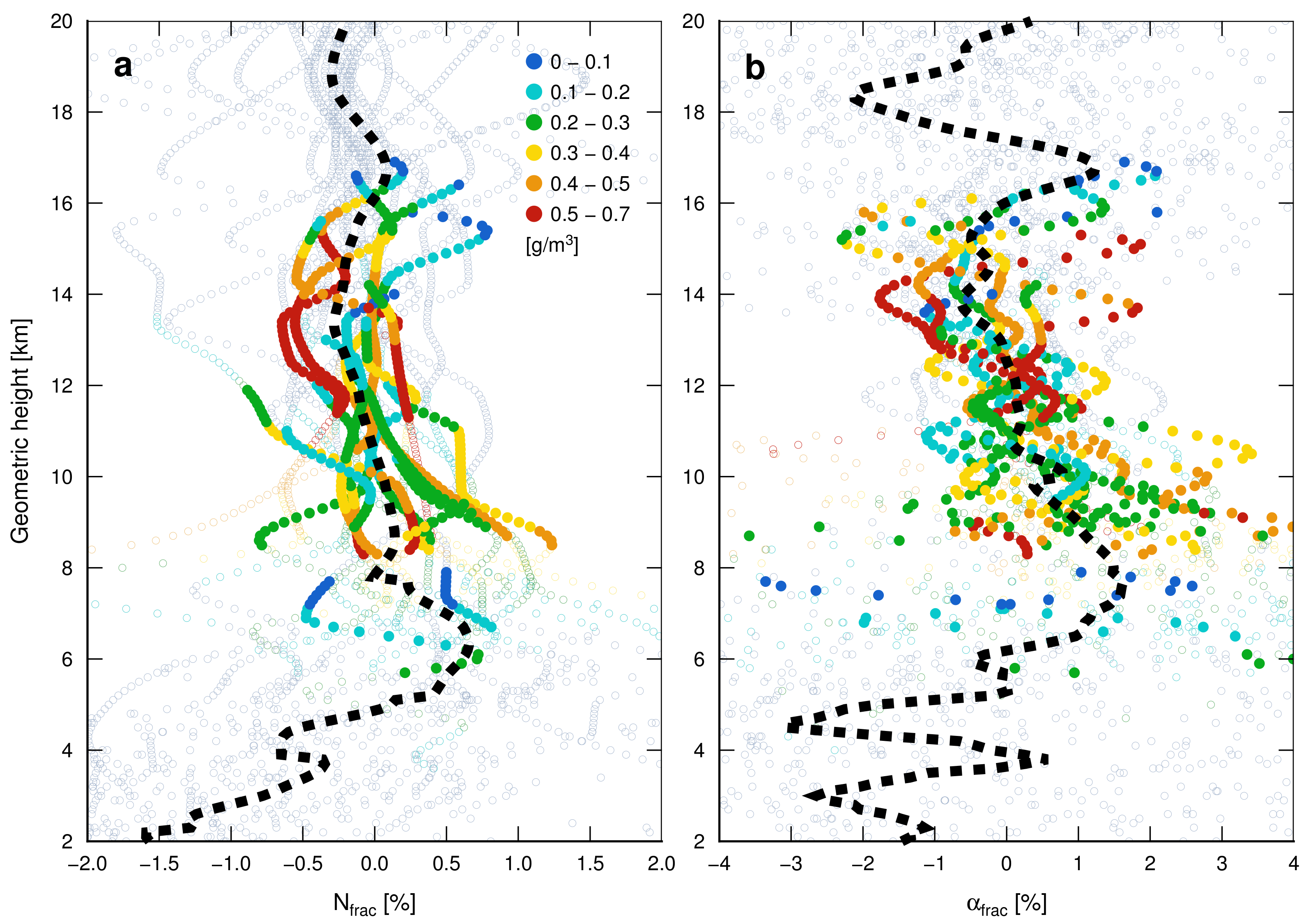
Figure 3a shows the fractional difference between refractivity from RO and ERA and the data are significant mostly in the range 8–17 km with a few cases below. Observations with significant cloud content (full dots) have mostly positive values within 6–11 km, especially around 7–9 km, as the mean fractional refractivity bias is more than 0.1%. For bending angle, the mean anomaly is 1.0%. Furthermore, the mean from all observations (within and outside uncertainty limits) is also greater than 0 in this range with a positive peak of 0.7% around 7 km height. Above 12 km, the mean value is slightly below zero, which can be influenced by a few greatly negative but unimportant observations.

In Figure 3b, we can see a positive bias of bending angle (${\alpha }_{frac}$) for most significant measurements within 8–14 km, where the largest bias is observed around 9 km. The mean value is positive within 6–13 km, with a maximum of 1.5% around 8 km, but we recognize a negative bias of almost 3%, where, at the same height, refractivity bias is positive (Figure 3a). However, as reported in [23], a bending angle bias induced by clouds follows the slight bias with the opposite sign and is not directly related to the cloud refractivity but to the vertical gradient of cloud refractivity. Furthermore, a fraction of cloud refractivity with 0.7% responds to bending angle error of almost 4%. It has to be pointed out here that, for the most intense case (red circles in Figure 3), the bending angle difference is positive.

4.2. Mean Cloud Contribution

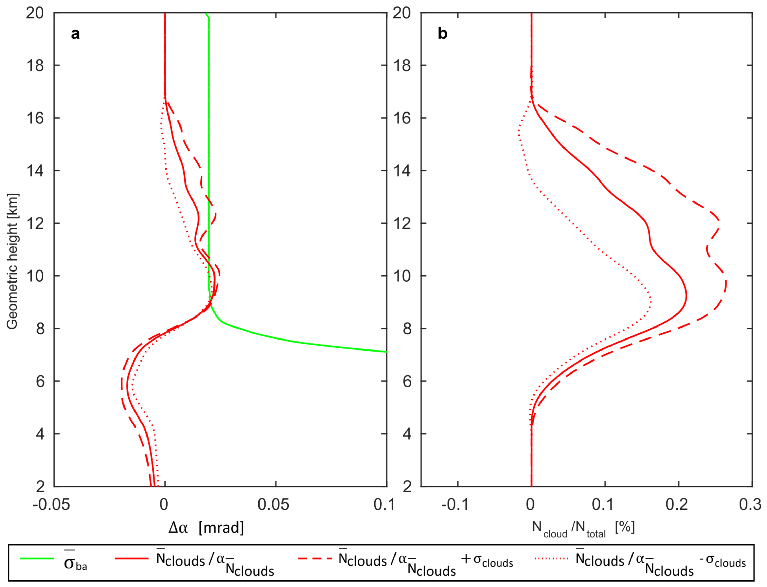
Comparisons of mean RO bending angle standard deviation provided by CDAAC in atmPrf for the whole investigated period (2007–2010) ${\sigma }_{ba}$ and differences between ERA plus CloudSat and ERA bending angle $\Delta \alpha$, with respect to height are presented in the Figure 4a.

The mean bending angle uncertainty ${\overline{\sigma }}_{ba}$ (Figure 4a) is lower than ${\alpha }_{{\overline{N}}_{clouds}-{\sigma }_{clouds}}$, ${\alpha }_{{\overline{N}}_{clouds}+{\sigma }_{clouds}}$ and ${\alpha }_{{\overline{N}}_{clouds}}$. The detection range starts from 9.0 to 10.5 km for mean cloud refractivity ${\alpha }_{{\overline{N}}_{clouds}}$ and spreads from 9.1 to 10.1 km (${\overline{N}}_{clouds}-{\sigma }_{clouds}$), while for ${\overline{N}}_{clouds}+{\sigma }_{clouds}$ the range is split into two ranges: 8.9–10.7 km and 11.8–12.9 km. This separation is an effect of the lower mean cloud contribution and especially its standard deviation. Since mean RO bending angle error greatly increases below 9.0 km, change in cloud content does not significantly alter the lower boundary. Furthermore, clouds’ influence on the bending angle is homogeneous within 8–8.5 km for ${\alpha }_{{\overline{N}}_{clouds}-{\sigma }_{clouds}}$, ${\alpha }_{{\overline{N}}_{clouds}+{\sigma }_{clouds}}$ and ${\alpha }_{{\overline{N}}_{clouds}}$.

Figure 4b shows percentage cloud contribution to the total refractivity with respect to height. For unmodified cloud refractivity (${\alpha }_{{\overline{N}}_{clouds}}$), fractional influence is approximately 0.2%, while, for ${\overline{N}}_{clouds}+{\sigma }_{clouds}$, it is over 0.3% around 9.5–12.0 km. Furthermore, we notice that maximum cloud contribution to the total refractivity is slightly over 0.7% (not shown). The reduced refractivity ${\overline{N}}_{clouds}-{\sigma }_{clouds}$ has values below zero between 13.0 and 17.0 km, which just indicates that, at these heights, there are no clouds after reduction. Moreover, the cloudy section in this profile, around 9.0 km, is slightly above the uncertainty level, hence the minimum detectable refractivity is 0.15% or more.

4.3. Cloud Detection Range

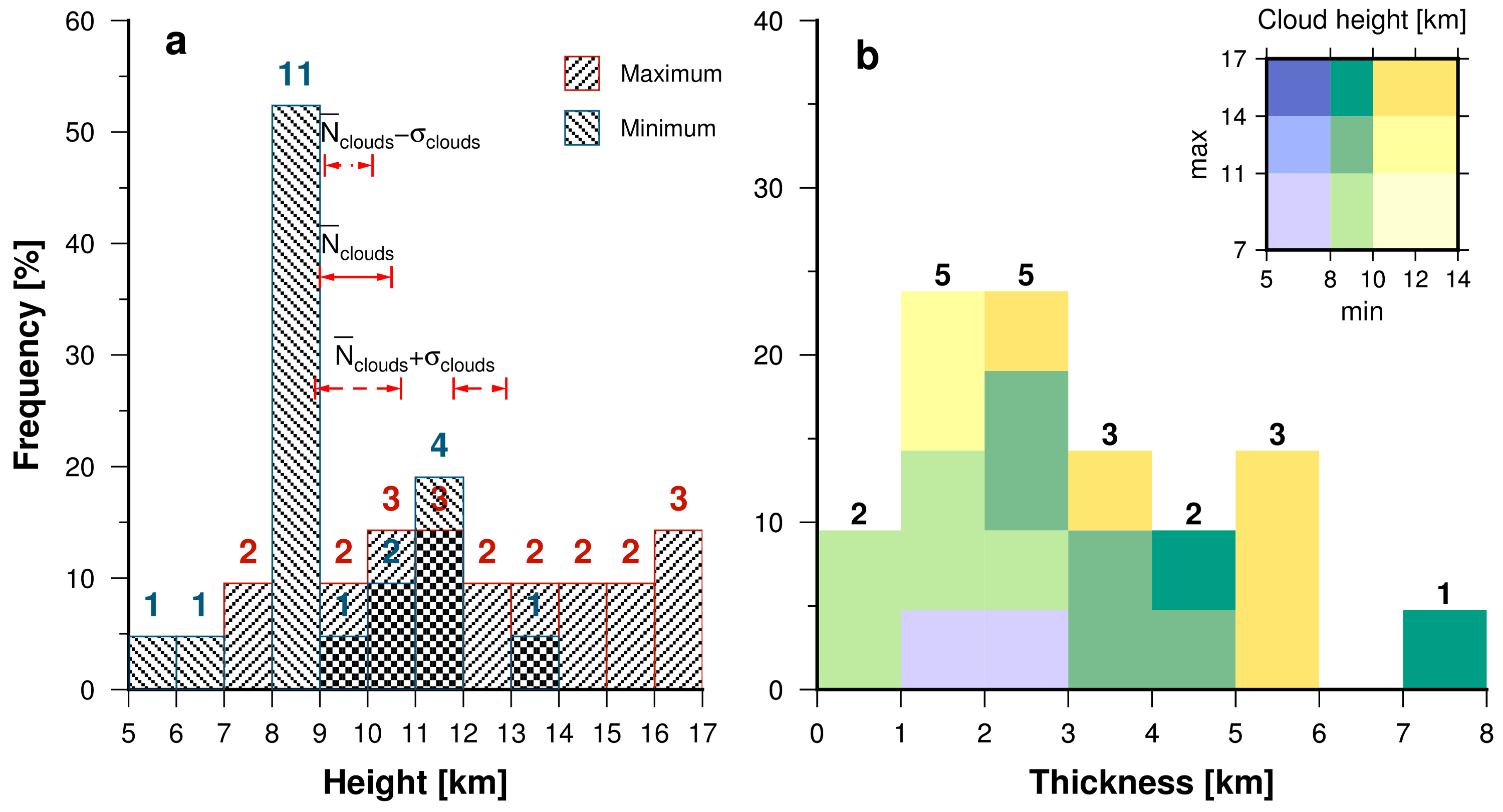
Figure 5a gives a histogram of minimum and maximum heights, providing upper and lower bound for cloud detection. More than half of the observations have a lower bound within 8–9 km, for two cases minimum height is within 5–7 km where each observation falls into a separate interval. Interestingly, more than one third of minimum heights are higher than 9 km, even though RO bending angle error rapidly decreases and is relatively small above 9.0 km. Figure 5a shows that the upper bound of detection range has an almost uniform distribution, which varies between one and three cases between 7 and 17 km. Only interval 8–9 km stands out as an empty class. Slightly under one third of the observations have their maximum heights within 12–14 km; however, more than one quarter of the results surpass this altitude with three observation events in the maximum interval 16–17 km. The same figure reports detection ranges for mean cloud contributions described in Section 4.2. It is clear that lower boundaries overlap with most frequent range for single cases. Interestingly, the lower boundary of the second range of ${\overline{N}}_{clouds}+{\sigma }_{clouds}$ shows similar dependency and coincides with the second most frequent class (11–12 km). Unfortunately, a similar pattern is not found for upper boundaries of detection ranges.

Minimum and maximum heights present only a location in space but do not reflect the thickness of layer where clouds are significant; hence, we combine together thickness and minimum and maximum heights (Figure 5b). From the histogram, we can note that almost 60% of the cases had a thickness below 3 km where the range 1–3 km stands out with a maximum number of observations. Moreover, most of these observations had minimum and maximum heights in ranges 8–10 km and 7–11 km, respectively. It is worth noting that detected cloud layer with the thickness above 7 km has minimum and maximum heights within 8–10 km and 14–17 km, respectively. Interestingly, maximum heights of low clouds with minimum heights below 8 km do not exceed 11 km and their thickness extends 1–3 km. Just slightly less than 10% of the observations have the thickness below 1 km, even though we rejected all cloud detection ranges with the thickness below 0.5 km.

5. Discussion

It is widely accepted that RO technique is insensitive to clouds. Our investigation, however, shows this assumption to be invalid in the case of dense clouds present in TC where 42% of profiles were affected by clouds. The altitudes of clouds’ detection ranges vary to some extent but more than half of them have the minimum height in range 8–9 km, which results from the rapid increase of mean RO bending angle error below this height and which implies clouds below 5 km are not detectable. Although maximum heights do not show such clear pattern, most of them do not exceed 14 km and three observations surpass 16 km, which is considered as minimum height of Cold Point Tropopause in tropics and end of Tropical Tropopause Layer [35]; hence, these clouds can be difficult to detect based only on temperature gradient. Furthermore, on average, the clouds’ detection range thickness is 1–3 km but for most of the observations detection range spreads from 8–10 km to 11–14 km. Interestingly, we observed slightly less than 10% of clouds with detection range thickness of 0.5–1 km, while one of the observations extends for 7–8 km.

In recent years, growing interest in cloud contribution to total refractivity derived from RO observations is observed. Zou et al. [22] demonstrated that mean ice cloud contribution to refractivity derived from CloudSat is over 0.1% above 8 km with the maximum impact of single clouds exceeding 0.6%. Our experiment is in line with these results, with mean contribution exceeding 0.1% (Figure 4b) and maximum around 0.7%. Furthermore, Yang and Zou [21] stated that the mean effect of the liquid part below 6 km is approximately 0.1% and we obtained negligible values (Figure 4b). There are a few possible explanations for these differences. First, we took into account whole profiles, not only parts between cloud bases and tops (as done in [21]), which can introduce zero cloud contribution of single profiles. Next, we investigated cases when the presence of precipitation-sized particles led to the divergence of the liquid water content solutions in the 2B-CWC-RO product and LWC data were unavailable. Finally, we only considered RO profiles, which passed our sensitivity test; hence, we could reject profiles with significant cloud contribution below 9 km because at this height observation noise greatly increased.

6. Conclusions and Future Work

This work demonstrates the clouds’ impact on Global Positioning System Radio Occultation (RO) bending angle profiles during TCs during 2007–2010. In this study, we analyzed RO bending angle sensitivity on potential cloud content derived from the CloudSat mission with respect to the bending angle noise provided by CDAAC. Our results reveal that the influence of clouds is visible in 21 out of 50 investigated cases and reaches up to 0.7% of total refractivity, with a mean of around 0.1%. Almost 15% of the observations with significant clouds’ impact reach a height of 16 km, which is considered to be the minimum height of tropical cold point tropopause.

We found that most of the RO observations which passed the proposed sensitivity test correspond well with positive fractional refractivity differences between RO and ERA at 6–11 km height. The largest mean bias of more than 0.5% is located around 7 km, although most of the RO profiles are not significant at this height due to large measurement uncertainty. A similar pattern but shifted up is visible in bending angle biases with a maximum mean fractional difference around 8 km. It is worth noting that positive bending angle bias follows the negative fractional differences and this change is related to the gradient of refractivity.

In our research, we focused on the period 2007–2010, when many RO and CloudSat observations were available. Currently, the number of available RO, as well as CloudSat measurements, is limited. CloudSat operates on a new orbit in daylight only, while COSMIC satellites experienced battery degradation and other technical issues. The launch of six COSMIC-2 satellites into low inclination orbits scheduled in 2018 shall provide us with around 6000 profiles per day. The growing number of observations will be used to investigate whether the bending angle differences could be applied to other, less intensive weather such as extratropical storms, squall lines, Mesoscale Convection Systems and others.

References

- Kursinski, E.; Hajj, G.; Schofield, J.; Linfield, R.; Hardy, K.R. Observing Earth’s atmosphere with radio occultation measurements using the Global Positioning System. J. Geophys. Res. Atmos. 1997, 102, 23429–23465. [Google Scholar] [CrossRef]
- Melbourne, W.; Davis, E.; Duncan, C.; Hajj, G.; Hardy, K.; Kursinski, E.; Meehan, T.; Young, L.; Yunck, T. The Application of Spaceborne GPS to Atmospheric Limb Sounding and Global Change Monitoring; Technical Report; Jet Propulsion Laboratory, California Institute of Technology: Pasadena, CA, USA, 1994. [Google Scholar]
- Gorbunov, M.; Lauritsen, K.; Rhodin, A.; Tomassini, M.; Kornblueh, L. Radio holographic filtering, error estimation, and quality control of radio occultation data. J. Geophys. Res. Atmos. 2006, 111. [Google Scholar] [CrossRef] [Green Version]
- Scherllin-Pirscher, B.; Steiner, A.; Kirchengast, G.; Kuo, Y.H.; Foelsche, U. Empirical analysis and modeling of errors of atmospheric profiles from GPS radio occultation. Atmos. Meas. Tech. 2011, 4, 1875–1890. [Google Scholar] [CrossRef] [Green Version]
- Kursinski, E.R.; Hajj, G.A.; Leroy, S.S.; Herman, B. The GPS radio occultation technique. Terr. Atmos. Ocean. Sci. 2000, 11, 53–114. [Google Scholar] [CrossRef]
- Biondi, R.; Randel, W.; Ho, S.P.; Neubert, T.; Syndergaard, S. Thermal structure of intense convective clouds derived from GPS radio occultations. Atmos. Chem. Phys. 2012, 12, 5309–5318. [Google Scholar] [CrossRef] [Green Version]
- Son, S.W.; Tandon, N.F.; Polvani, L.M. The fine-scale structure of the global tropopause derived from COSMIC GPS radio occultation measurements. J. Geophys. Res. Atmos. 2011, 116. [Google Scholar] [CrossRef] [Green Version]
- Randel, W.J.; Wu, F. Kelvin wave variability near the equatorial tropopause observed in GPS radio occultation measurements. J. Geophys. Res. Atmos. 2005, 110. [Google Scholar] [CrossRef] [Green Version]
- Shultz, J.M.; Russell, J.; Espinel, Z. Epidemiology of tropical cyclones: The dynamics of disaster, disease, and development. Epidemiol. Rev. 2005, 27, 21–35. [Google Scholar] [CrossRef] [PubMed]
- Pielke, R.A., Jr.; Pielke, R.A., Sr. Hurricanes: Their Nature and Impacts on Society; John Wiley and Sons: Chichester, UK, 1997. [Google Scholar]
- Anthes, R. Tropical Syclones: Their Evolution, Structure and Effects; American Meteorological Society: Boston, MA, USA, 1982. [Google Scholar]
- Dvorak, V.F. Tropical cyclone intensity analysis and forecasting from satellite imagery. Mon. Weather Rev. 1975, 103, 420–430. [Google Scholar] [CrossRef]
- Vergados, P.; Luo, Z.J.; Emanuel, K.; Mannucci, A.J. Observational tests of hurricane intensity estimations using GPS radio occultations. J. Geophys. Res. Atmos. 2014, 119, 1936–1948. [Google Scholar] [CrossRef] [Green Version]
- Luo, Z.; Stephens, G.L.; Emanuel, K.A.; Vane, D.G.; Tourville, N.D.; Haynes, J.M. On the use of CloudSat and MODIS data for estimating hurricane intensity. IEEE Geosci. Remote Sens. Lett. 2008, 5, 13–16. [Google Scholar]
- Houze, R.A., Jr. Clouds in tropical cyclones. Mon. Weather Rev. 2010, 138, 293–344. [Google Scholar] [CrossRef]
- Romps, D.M.; Kuang, Z. Overshooting convection in tropical cyclones. Geophys. Res. Lett. 2009, 36. [Google Scholar] [CrossRef] [Green Version]
- Fueglistaler, S.; Dessler, A.; Dunkerton, T.; Folkins, I.; Fu, Q.; Mote, P.W. Tropical tropopause layer. Rev. Geophys. 2009, 47. [Google Scholar] [CrossRef] [Green Version]
- Biondi, R.; Ho, S.P.; Randel, W.; Syndergaard, S.; Neubert, T. Tropical cyclone cloud-top height and vertical temperature structure detection using GPS radio occultation measurements. J. Geophys. Res. Atmos. 2013, 118, 5247–5259. [Google Scholar] [CrossRef] [Green Version]
- Biondi, R.; Steiner, A.; Kirchengast, G.; Rieckh, T. Characterization of thermal structure and conditions for overshooting of tropical and extratropical cyclones with GPS radio occultation. Atmos. Chem. Phys. 2015, 15, 5181–5193. [Google Scholar] [CrossRef] [Green Version]
- Lin, L.; Zou, X.; Anthes, R.; Kuo, Y.H. COSMIC GPS radio occultation temperature profiles in clouds. Mon. Weather Rev. 2010, 138, 1104–1118. [Google Scholar] [CrossRef]
- Yang, S.; Zou, X. Assessments of cloud liquid water contributions to GPS radio occultation refractivity using measurements from COSMIC and CloudSat. J. Geophys. Res. Atmos. 2012, 117. [Google Scholar] [CrossRef] [Green Version]
- Zou, X.; Yang, S.; Ray, P. Impacts of ice clouds on GPS radio occultation measurements. J. Atmos. Sci. 2012, 69, 3670–3682. [Google Scholar] [CrossRef]
- Hordyniec, P. Simulation of liquid water and ice contributions to bending angle profiles in the radio occultation technique. Adv. Space Res. 2018, 62, 1075–1089. [Google Scholar] [CrossRef]
- Sokolovskiy, S.; Schreiner, W.; Rocken, C.; Hunt, D. Optimal noise filtering for the ionospheric correction of GPS radio occultation signals. J. Atmos. Ocean. Technol. 2009, 26, 1398–1403. [Google Scholar] [CrossRef]
- Gorbunov, M.E.; Lauritsen, K.B. Error estimate of bending angles in the presence of strong horizontal gradients. In New Horizons in Occultation Research; Springer: Berlin/Heidelberg, Germany, 2009; pp. 17–26. [Google Scholar]
- Sokolovskiy, S. Improvements, modifications and alternative approaches in the processing of GPS RO data. In Proceedings of the 5th ROM SAF User Workshop on Applications of GPS Radio Occultation Measurements, Reading, UK, 16–18 June 2014. [Google Scholar]
- Dee, D.P.; Uppala, S.M.; Simmons, A.; Berrisford, P.; Poli, P.; Kobayashi, S.; Andrae, U.; Balmaseda, M.; Balsamo, G.; Bauer, D.P.; et al. The ERA-Interim reanalysis: Configuration and performance of the data assimilation system. Q. J. R. Meteorol. Soc. 2011, 137, 553–597. [Google Scholar] [CrossRef]
- CDAAC: COSMIC Data Analysis and Archive Center. CDAAC Description. Available online: https://cdaac-www.cosmic.ucar.edu/cdaac/cgibin/fileFormats.cgi?type=eraPrf (accessed on 13 August 2018).
- Bao, X.; Zhang, F. Evaluation of NCEP–CFSR, NCEP–NCAR, ERA-Interim, and ERA-40 reanalysis datasets against independent sounding observations over the Tibetan Plateau. J. Clim. 2013, 26, 206–214. [Google Scholar] [CrossRef]
- Tanelli, S.; Durden, S.L.; Im, E.; Pak, K.S.; Reinke, D.G.; Partain, P.; Haynes, J.M.; Marchand, R.T. CloudSat’s cloud profiling radar after two years in orbit: Performance, calibration, and processing. IEEE Trans. Geosci. Remote Sens. 2008, 46, 3560–3573. [Google Scholar] [CrossRef]
- Wu, D.; Austin, R.; Deng, M.; Durden, S.; Heymsfield, A.; Jiang, J.; Lambert, A.; Li, J.L.; Livesey, N.; McFarquhar, G.; et al. Comparisons of global cloud ice from MLS, CloudSat, and correlative data sets. J. Geophys. Res. Atmos. 2009, 114. [Google Scholar] [CrossRef] [Green Version]
- Knapp, K.R.; Kruk, M.C.; Levinson, D.H.; Diamond, H.J.; Neumann, C.J. The International Best Track Archive for Climate Stewardship (IBTrACS) Unifying Tropical Cyclone Data. Bull. Am. Meteorol. Soc. 2010, 91, 363–376. [Google Scholar] [CrossRef]
- Atkinson, G.D. Investigation of Gust Factors in Tropical Cyclones; Technical Report; Fleet Weather Central/Joint Typhoon Warning Center: San Francisco, CA, USA, 1974. [Google Scholar]
- Smith, E.K.; Weintraub, S. The constants in the equation for atmospheric refractive index at radio frequencies. Proc. IRE 1953, 41, 1035–1037. [Google Scholar] [CrossRef]
- Gettelman, A. A climatology of the tropical tropopause layer. J. Meteorol. Soc. Jpn. Ser. II 2002, 80, 911–924. [Google Scholar] [CrossRef]
Figure 1.
Global distribution of tropical cyclone tracks provided by IBTrACS with collocated 50 RO-CloudSat pairs during 2007–2010. Colored lines denote intensities of TC according to Saffir–Simpson Hurricane Intensity Scale, while circles indicate RO profiles. Profiles which passed sensitivity test (Equation (8)) are highlighted in red.
Figure 3.
All fractional N differences (a); and bending angle differences (b) for 21 cases for which Equation (5) holds (dots). Empty circles represent the bending angle value exceeding the uncertainty of bending angle retrieval, dots within the uncertainty limits. Dashed black line is a mean of all differences in the experiment. Colors represent IWC intensity (from blue to red in gm).
Figure 4.
(a) Average bending angle residuals (BA computed from ERA data with and without cloud parameters from CloudSat) over the 21 cases described in Section 4.3 with respect to modified cloud refractivity; and (b) mean fractional clouds contribution to the total ERA refractivity.
Figure 5.
Histograms for single clouds’ detection ranges: (a) minimum (blue) and maximum (red) heights; and (b) thickness of these ranges. Horizontal lines in (a) present detection ranges for mean cloud contribution described in Section 4.2. In (b), colors indicate minimum and maximum ranges of heights where cloud’s impact was significant. The numbers above bars indicate the number of observations.
© 2018 by the authors. Licensee MDPI, Basel, Switzerland. This article is an open access article distributed under the terms and conditions of the Creative Commons Attribution (CC BY) license (http://creativecommons.org/licenses/by/4.0/).
Share and Cite
MDPI and ACS Style
Lasota, E.; Rohm, W.; Liu, C.-Y.; Hordyniec, P. Cloud Detection from Radio Occultation Measurements in Tropical Cyclones. Atmosphere 2018, 9, 418. https://doi.org/10.3390/atmos9110418
AMA Style
Lasota E, Rohm W, Liu C-Y, Hordyniec P. Cloud Detection from Radio Occultation Measurements in Tropical Cyclones. Atmosphere. 2018; 9(11):418. https://doi.org/10.3390/atmos9110418
Chicago/Turabian StyleLasota, Elżbieta, Witold Rohm, Chian-Yi Liu, and Paweł Hordyniec. 2018. "Cloud Detection from Radio Occultation Measurements in Tropical Cyclones" Atmosphere 9, no. 11: 418. https://doi.org/10.3390/atmos9110418
Note that from the first issue of 2016, this journal uses article numbers instead of page numbers. See further details here.