Flash Flood Forecasting in São Paulo Using a Binary Logistic Regression Model


Department of Atmospheric Sciences, University of São Paulo, São Paulo 05508-090, Brazil
*
Author to whom correspondence should be addressed.
Atmosphere 2020, 11(5), 473; https://doi.org/10.3390/atmos11050473
Submission received: 15 February 2020
/
Revised: 23 March 2020
/
Accepted: 24 March 2020
/
Published: 7 May 2020
(This article belongs to the Special Issue Atmospheric Radar for Severe Weather Surveillance and Analysis)
Abstract
:This study presents a flash flood forecasting model that uses a binary logistic regression method to determine the occurrence of flash flood events in different watersheds in the city of São Paulo, Brazil. This study is based on two years (2015–2016) of rain estimates from a dual-polarization S-band Doppler weather radar (SPOL) and flood locations observed by the Climate Emergency Management Center (CGE) of São Paulo City Hall. The logistic regression model is based on daily accumulated precipitation, a maximum precipitation rate, and daily rainfall duration. The model presented a probability of detection (POD) of 46% (71%) on average for flood events (conditional), while, for events without flash flood, it reached 98% probability. Despite the low averaged POD for flash flood occurrence, the model demonstrated a good performance for watersheds located in the east of the city near the Tietê River and in the southeast with probabilities above 50%.
1. Introduction
Currently, more people are affected by flash floods than any other type of natural disaster [1,2,3]. In recent years, the most populated cities have been affected by floods and flash floods that directly or indirectly impact the socioeconomic development of the population. For example, São Paulo, known as the most populated city in Brazil, has frequent flash floods caused by several factors that are sometimes related to the hydrographic basin, local catchments, and local effects like the topography and soil coverage. In the summer of 2014/2015, the traffic vehicle department of São Paulo observed 183 flooding points, and 130 flooding events occurred between January and March 2015.
To reduce hydro-geological risk from flash floods, several studies have implemented methodologies that monitor and analyze the behavior of rainfall to implement a flash flood warning system. Flash flood forecasting algorithms are commonly based on hydrological or hydraulic models [4,5,6,7], numerical simulation models [3,8,9,10], and Machine Learning algorithms such as the Artificial Neural Network [11,12,13,14], Support Vector Machines [15], Adaptive Neuro-Fuzzy Inference Systems (ANFIS) [16], or Random Forest [2,17]. Likewise, Mosavi et al. [18] demonstrated the advantages of certain Machine Learning algorithms through a qualitative analysis. In this study, they considered the flood resource variable, such as water levels, precipitation or streamflow, and the prediction type. Based on the correlation coefficient (R2) and root mean square error (RMSE) evaluation, they concluded that combining two or more methods, by using data decomposition techniques or using add-on optimizer algorithms, improve the flood prediction for short-term and long-term predictions.
However, there are hardly any studies on flash flood forecasting using regression applications as they are usually focused on a numerical forecasting of flash flood events [19]. The logistic regression with a binary response is simply a designation of one of two possible outcomes. It means that we have a prediction of a chance or a probability. Studies in landslides [20,21] or hail risk [22,23] demonstrate the efficiency of logistic regression for predicting the probability of occurrence.
In São Paulo city, the Flood Alert System of São Paulo (SAISP), operated by the Technological Center of the Hydraulics Foundation (FCTH), monitors flood events by integrating a dual-band S Doppler radar polarization and telemetry. For flood forecasting, SAISP uses a hydrological model called SWMM (Storm Water Management Model) that generates flood maps and shows affected areas in the São Paulo Metropolitan Region (RMSP) [24]. The model was validated by Sosnoski et al. [25], and the results showed that it can be a useful tool for delimiting flood areas. This information is reported to various agencies, especially to the Climate Emergency Management Center (CGE), which also gathers information from weather stations, rain gauges, and local observations in order to monitor the points of the flood.
According to the study of Viteri [26], who used radar measurements with flash flood events and points, flash flood events in São Paulo are associated with a rainfall volume greater than 30 mm per day and a maximum rainfall rate greater than 30 mmh−1. Furthermore, neighborhoods located near the Tietê and Pinheiros rivers and in the central region of São Paulo city presented higher probability of the occurrence of flash floods when there were rainfall volumes lower than the average of 30 mm per day in addition to presenting a higher recurrence of flood points.
Based on these features, this study aims to estimate the probability of occurrence of flash floods in São Paulo city considering its watersheds. In order to do this, the study presents a binary logistic regression model that combines rain estimates from the dual-polarization S-band Doppler meteorological weather radar (SPOL) from the Departamento de Águas e Energia Elétrica (DAEE) and the FCTH and flooding points observed by the CGE during the occurrence/non-occurrence of flash flood events.
2. Data and Methodology
2.1. Study Area
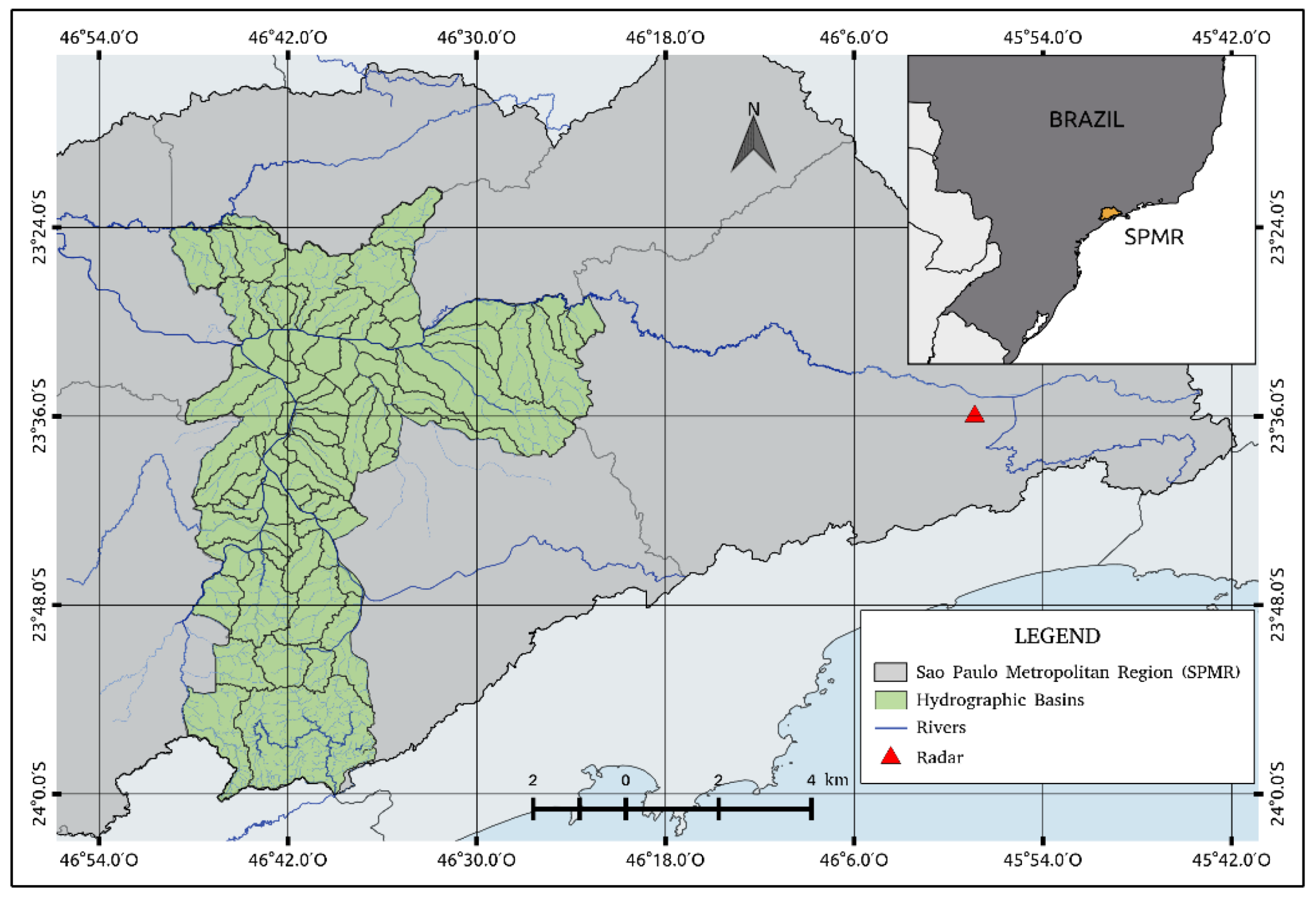
The study area is the city of São Paulo located in the state of São Paulo in Southeast Brazil. São Paulo is the biggest city of São Paulo Metropolitan Region (SPMR) with an area of 1521 km2 and approximately 12.1 million people. SPMR includes 39 municipalities and represents the largest industrial complex and urban concentration in Latin America [24].
The city of São Paulo is divided into 96 districts with a mean altitude of 760 m along the Tietê River basin, which is divided into Upper, Middle, and Lower Tietê and is the major water source of SPMR. The Upper Tietê river basin, where the city of São Paulo is located, has a drainage area of 5720 km2. There are seven dams in which two control the Tietê river flow, and the other five contribute to the Upper Tietê Producer System in SPMR. The Ponte Nova Dam, which is located in Southeast SPMR, has the major drained area of 320 km2 with a discharge of 3.9 m3/s, which is followed by Taiaçupeba with 224 km2 drained area and 0.5 m3/s discharge.
In total, São Paulo has more than 300 rivers (surface and canalized) that form the relief of each watershed. The Pinheiros and Tamanduateí rivers are the main tributaries of the Tietê river in the topography of 186 watersheds in the city, as seen in Figure 1. For example, the Aricanduva river is located in the eastern region of São Paulo and has an approximate drained area of 100.4 km2. The Pirajucara river, which is located in the western zone, has a drained area of 72 km2. The Mandaqui river is a basin located in the northern region of the city that is almost completely urbanized, and has a drained area of 18.6 km2 [5].
Cold fronts, squall lines, sea breezes, and local convection are the main meteorological systems contributing to precipitation in the city of São Paulo and surrounding areas [26]. Annually, São Paulo has a precipitation of more than 1200 mm, and, during summer time (December-March), it varies from 450 mm to 700 mm. Due to the large number of impermeable areas, which increase the surface runoff, flash floods are frequent every year [27], especially in the rainy season, from October to March.
2.2. Rainfall Measurements
This study uses rain estimates obtained from a dual-polarization S-band Doppler weather radar (SPOL), model METEOR 600S from Selex, operated by the DAEE and the FCTH at the Ponte Nova dam, 70 km from São Paulo (Figure 1) for the 2015–2016 period. This radar is configured to scan a 240-km radius every 5 min with eight elevations, and with a gate resolution of 250 m.
For this study, we used the Dual Polarization Surface Rainfall Intensity (DPSRI) algorithm [28] to retrieve the rain estimates with a resolution of 500 × 500 m. In summary, the DPSRI algorithm uses radar reflectivity (Z), differential reflectivity (ZDR), and the specific differential phase (KDP) variables to estimate the rainfall rate in a Pseudo-DPSRI mode [29].
According to Viteri [30], the rainfall estimates used in this study were compared to a rain gauge network and presented a bias score (BIAS) of 31% for 10 min, 50% for one hour, and 89% for one day integration time. The RMSE varies from 16.3 mm for 10 min, 0.5 mm for one hour, and 6.6 mm for one day. The correlation coefficient provides a better fit for a timescale of one day, i.e., 0.8, which is followed by one hour with 0.7 and finally for 10 min with 0.4. Therefore, 24 h accumulated precipitation represents the best SPOL weather radar rain estimates.
2.3. Flash Flood Measurements
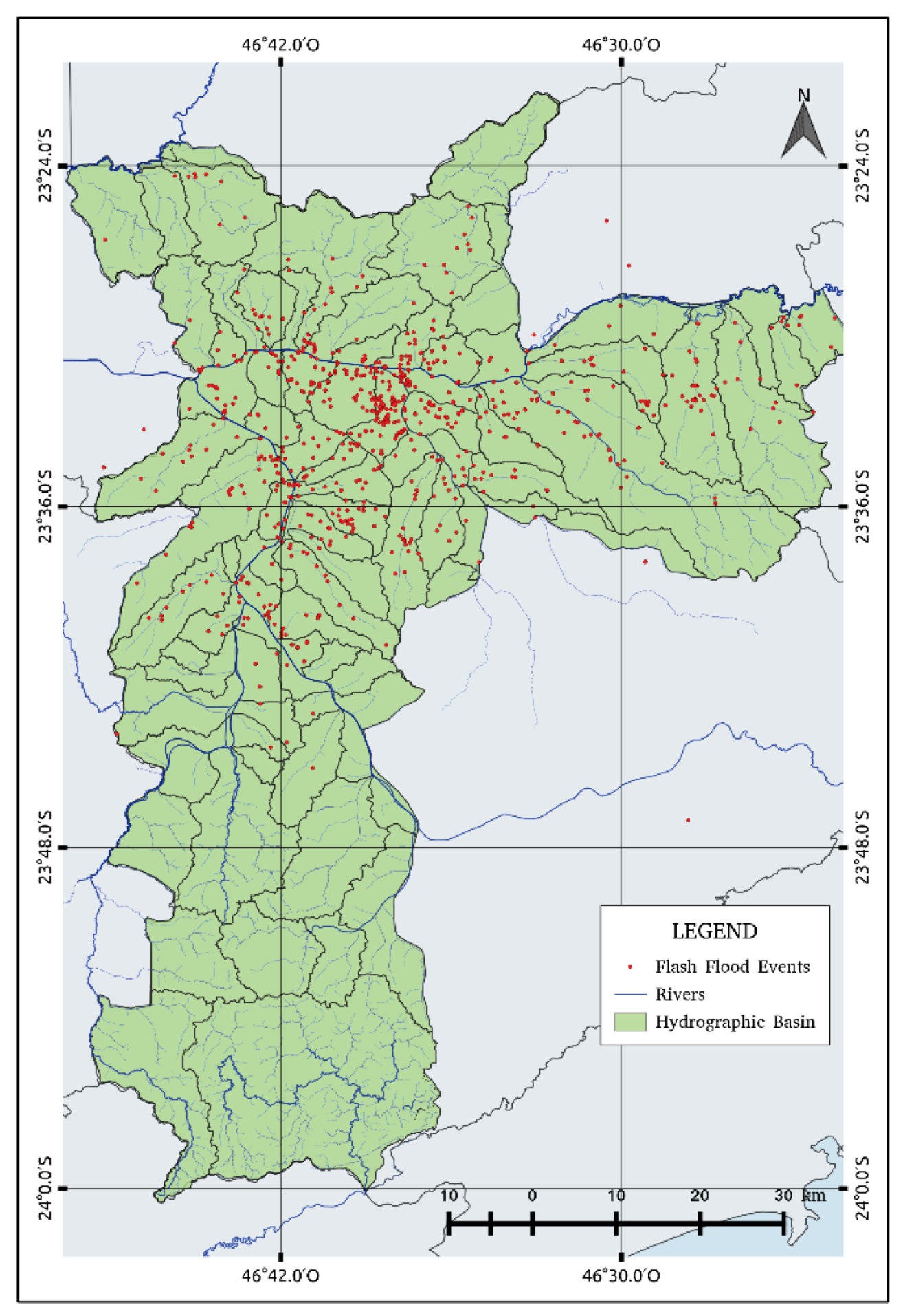
According to the National Center for Risk and Disaster Management (CENAD) [31], floods are hydrological phenomena caused by an excess capacity of surface runoff and urban drainage systems forming accumulations of water in impermeable areas. Faced with the chaotic urban expansion process, recurrent floods are observed in areas that lack favorable conditions for infiltration and runoff. For instance, during the summertime, São Paulo is frequently affected by flash floods that have tremendous economic impacts and increase the vulnerability of various neighborhoods with poor infrastructures. For example, Figure 2 shows the location of recorded flash floods in the period of 2015 and 2016. Most of the flash floods are observed along the Pinheiros and Tietê rivers as well as in other regions except for the southern region that does not show any events due to the absence of observations [26]. In 2015, there were 224 days with rain and 100 flood events, while, in 2016, there were 214 rainy days and 110 inundations.
To overcome this recurrent problem, São Paulo City Hall deployed the Climate Emergency Management Center (CGE) to monitor flood areas in the city of São Paulo and mitigate the effects. Basically, the CGE uses the SPOL radar and rain gauge measurements available from the FCTH and flood indications provided by the Municipal Civil Defense Coordination (COMDEC) and the Traffic Engineering Company (CET). For this study, we have used a flood inventory database from 2015 to 2016 provided by the CGE to adjust a binary logistic regression model to predict floods. The database contains the location, time of the occurrence, and a description of the events whenever available.
2.4. Binary Logistic Regression Model
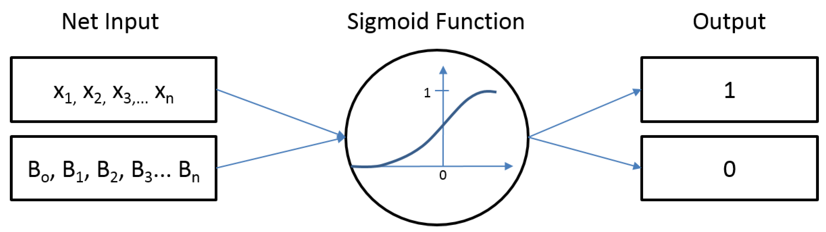
The probability of the occurrence of flash floods was obtained by the logistic regression model [32] (Figure 3) described on Equations (1–3). The logistic regression analyzes the association between two qualitative variables, which include one dependent variable and one independent variable (exploratory), without assuming a linear relationship. The dependent variable has only two values, such as presence or absence, success or failure, or an event occurring or not occurring. The independent variable can be continuous, discrete, or both [21,33]. The predictable output variable calculated has values of 0 or 1. For this study, zero means 0% probability of flash flood occurrence and one means 100% probability of flash flood occurrence.
The logistic regression model is based on the logistic function f(z), which is defined as:
where z is the net input, that is, the linear combination of weights (β) and sample features (x) and can be calculated by the equation below.
In terms of probability, this function can be written by the logit transformation, which has a relatively simple mathematical form.
where the odds ratio or likelihood ratio and p(x) are the probabilities of the event occurrence. Instead of using the least squared deviations for the best fit, the coefficients β are estimated by using the maximum likelihood method, which maximizes the probability of occurrence of flash floods given the fitted regression coefficients.
2.5. Methodology
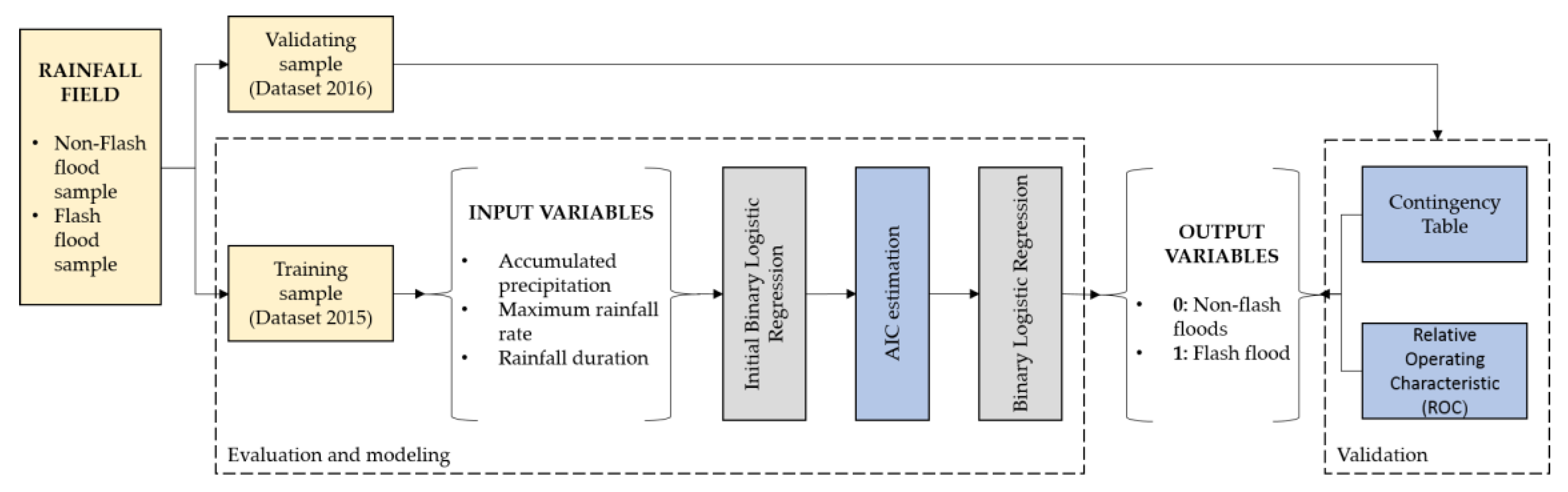
Figure 4 shows a flowchart of how the model is configured. First, the rainfall field measurements are obtained from the SPOL DPSRI algorithm. Second, the model uses daily accumulated precipitation, the maximum precipitation rate [mm/h], and total rainfall duration [min] registered in the previous 24 h.
To increase the number of samples and also to be equally distributed, the rainfall and flood database was divided into two sets: 2015 was used to adjust the model while 2016 was used for validation. Both datasets have flash flood and non-flash flood events. Finally, it is important to observe that the model output values vary from 0 to 1. Days with no occurrence of flash floods have been assigned to have a probability lower than 0.5, and those with a flash flood above 0.5.
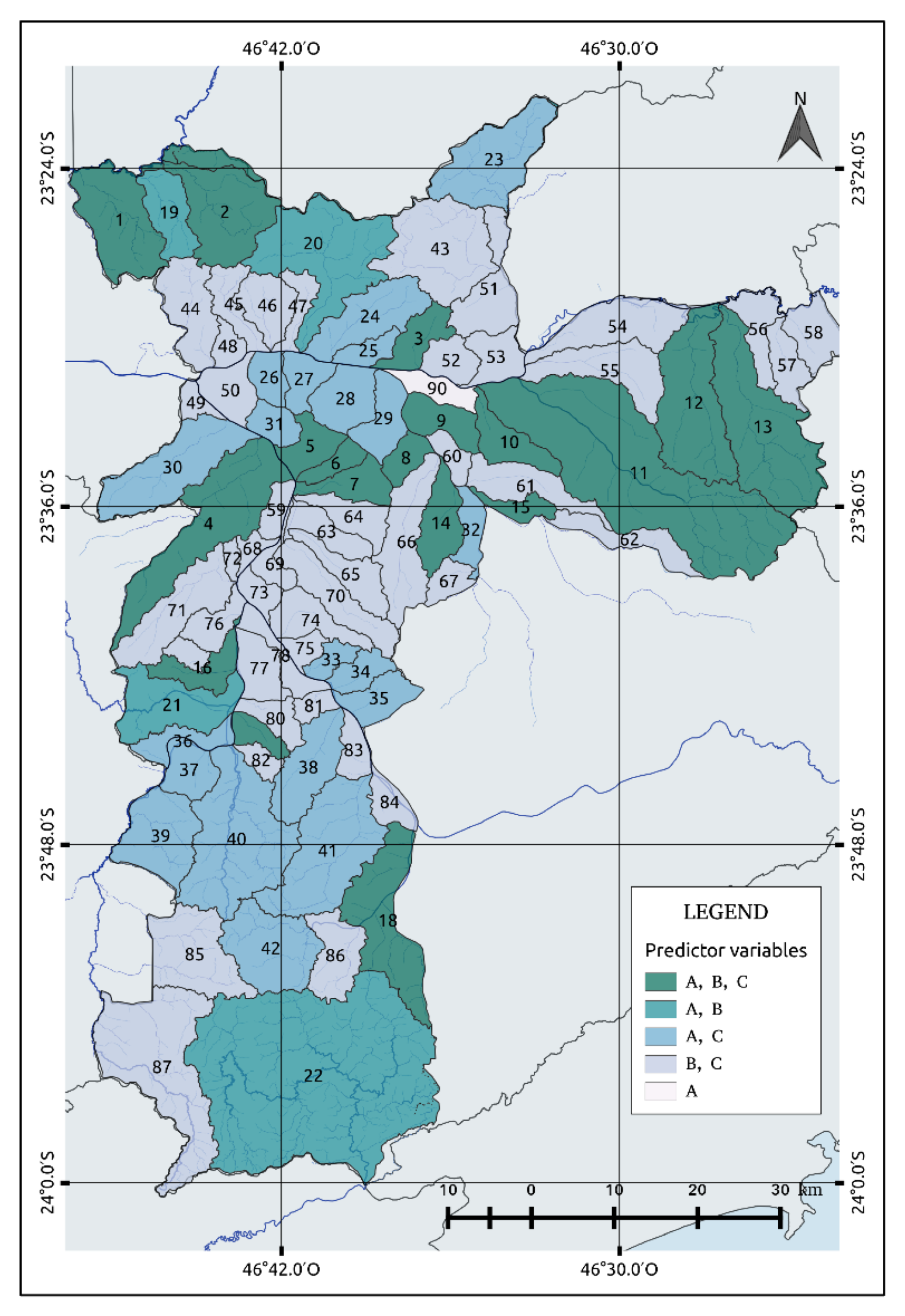
Moreover, in order to improve the accuracy of the probability, we applied the Akaike Information Criterion (AIC) [34] to select the best predictor variables for each watershed. Good model performance is that which has the minimum AIC value of all other model combinations. In our case, we can have seven combinations (Table 1) including three, two, and one predictor variables (A: Accumulated precipitation, B: maximum precipitation rate, and C: rainfall duration). For the example shown in Table 1, the maximum AIC had three and two variables A–C, while variable B presents the lowest AIC value. Therefore, variable B (maximum precipitation) represents the best variable to predict flash floods.
Lastly, in order to validate the logistic model, we employed the contingency table [35] method to compute the bias score (BIAS), the probability of detection (POD), the false alarm ratio (FAR), and the critical success index (CSI).
The BIAS is an indicator of how well the estimate predicts the number of occurrences of an event. The POD is defined as the percentage of correct answers when estimating the occurrence of the event, and it varies from 0 to 1, where 1 means the optimal performance. The POD is commonly known as the hit rate. The FAR is defined as the percentage in which the event did not occur and varied between 0 and 1. Furthermore, 0 means the best performance. The CSI index is defined as the percentage of correct answers in the estimates, and it varies between 0 and 1, with higher values representing better performance. In addition, the POD and FAR were combined to compute the Relative Operating Characteristic (ROC) [36] in order to verify the probabilistic forecast and to understand issues related to accuracy, criterion selection, and interpretation [21].
3. Results
In 2015 and 2016, more than 2000 flash flood points were registered by the CGE. Flash flood warnings were more frequent in the summertime, and were concentrated in the western, southern, and central regions of the city of São Paulo with a great number of recurrent locations (Figure 2).
In this study, we have considered only 90 watersheds that registered more than two flood points in order to estimate the probability of the occurrence of flash floods. Figure 5 summarizes the watershed selected with an indication of the number of predictor variables and respective index to consult the model coefficients (Appendix A, Table A1, Table A2, Table A3, Table A4 and Table A5). As explained in the previous section, AIC criteria were used to determine the best predictor variables to predict flash floods.
After the model validation, we obtained the predictor variables for each watershed and computed the probability by using Equation (4). For instance, the model uses the following parameters (): () accumulated precipitation, () maximum precipitation rate, and () rainfall duration together with the coefficients () calculated from the logistic regression model presented in Appendix A.
Moreover, Table A1, Table A2, Table A3, Table A4 and Table A5 in Appendix A also shows the accuracy of each watershed model. The accuracy ranged from 80 to 98% with a mean value of 86%. The p-values associated with the correlation of variables in each model are very small in some cases, which indicates their good association with the probability of flash floods. A significant p-value was found in 96% of the watersheds with a value of less than 0.8. Taking into account the rain estimates errors found by Viteri [26], the uncertainty of the model in predicting the probability will be less than 10–5 and, therefore, would not affect the flash flood prediction.
Analyzing Figure 5, it is possible to observe that most of the watersheds can be adjusted by two variables, i.e., maximum precipitation rate and rainfall duration (B,C), which is followed by 20 watersheds that use daily precipitation and rainfall duration (A,C), and four watersheds with accumulated precipitation and a maximum precipitation rate (A,B). Eighteen watersheds need the three variables, while only one watershed depends on only one variable, i.e., accumulated precipitation. Watersheds related to the predictor A tend to have flash flood occurrence with an average of 20 mm per day. Predictor B did not show any significant pattern. The highest values registered were located in the south, and two or three watersheds in the north and central regions (watersheds index 9, 18, 20, 21, 22, 42, and 60) with an average of 190 mm/h. Predictor C, on the other hand, is related to shorter rainfall durations since the maximum values were located in the watersheds not associated with this predictor variable.
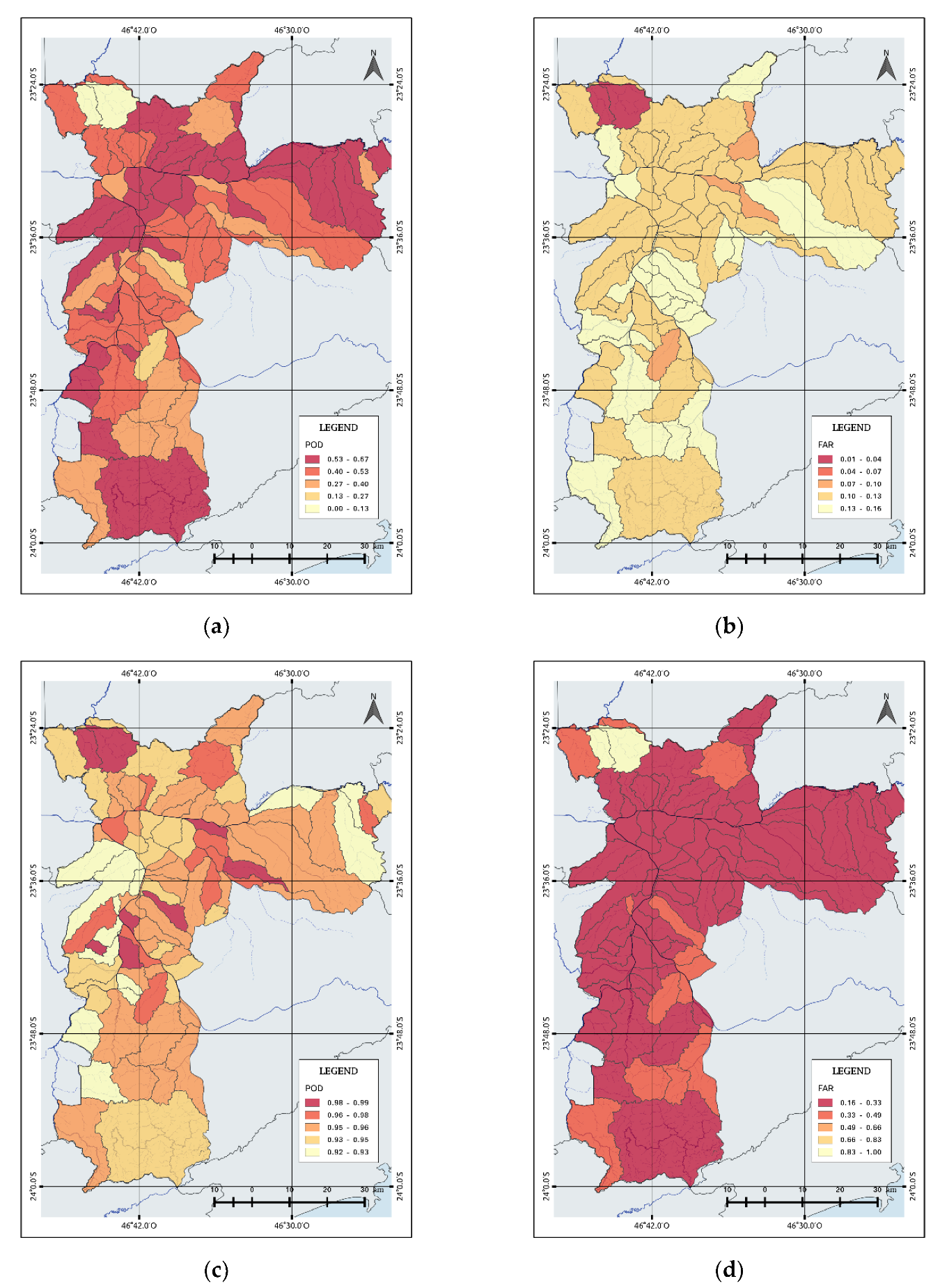
Figure 6 presents how the POD and FAR vary as functions of flash flood occurrence in each watershed. For flash flood events, the mean POD was 0.46, and the FAR was 0.12. The POD (Figure 6a) and FAR (Figure 6b) spatial distribution maps show several regions with acceptable performance (POD > 0.5). Watersheds with a lower POD are observed in the northern part of the city with a POD, but with a higher probability of non-flash flood occurrence (Figure 6c). These watersheds correspond to the Jaraguá and Perus neighborhoods, which registered 7 (1) and 1 (4) days with flash flood events, respectively, in 2015 (2016) at a maximum precipitation rate of 59 mm/h. Almost 48% of the watersheds located in the eastern part of the city and near the Tietê and Pinheiros Rivers, presented more than 50% POD that could be related to their recurrent flash flood events and the different infiltration capacity [30], which means ground capacity to absorb rain water.
The FAR map increases from 0.01 to 0.16 and demonstrates that few watersheds have predicted flash flood events that were not observed. For example, two watersheds located in the north obtained a good FAR value while 30% of the watersheds showed the FAR varying from 0.13 to 0.16. Most of them are concentrated in the south.
On the other hand, the POD and FAR for no occurrence of flash floods events (Figure 6c,d), respectively, show better results. The POD increases from 0.92 to 1 while the mean FAR is 0.297 (Table 2). According to Figure 6c, near the Tietê River, the probability of non-flash flood occurrence is higher, particularly in the neighborhoods of Pari and Belém, with a probability of 99%. At the edge of the River Pinheiros, we can observe watersheds with the high probability of non-occurrence, like Santo Amaro and Itaim Bibi, which registered 25 and 5 days with flash flood events. On the other hand, low POD values were observed in the eastern and southwestern districts and ranged from 0.92 to 0.93.
Moreover, Table 2 presents the average scores for events with and without flash flood occurrence using conditional (only rainy days) and unconditional rainy days (all days). From these scores, it is possible to note that the proposed model has a better performance to predict no flash flood events (BIAS, POD, and CSI), but, when only rain days are used, the model improved the prediction of flash flood events to 71%.
Comparing the average scores calculated for both situations, the logistic model has a better performance to predict the non-occurrence of flash floods (POD and CSI) even though it is possible to predict flash flood events with a 71% success rate when considering only rainy days.
Case Study: 11 March 2016
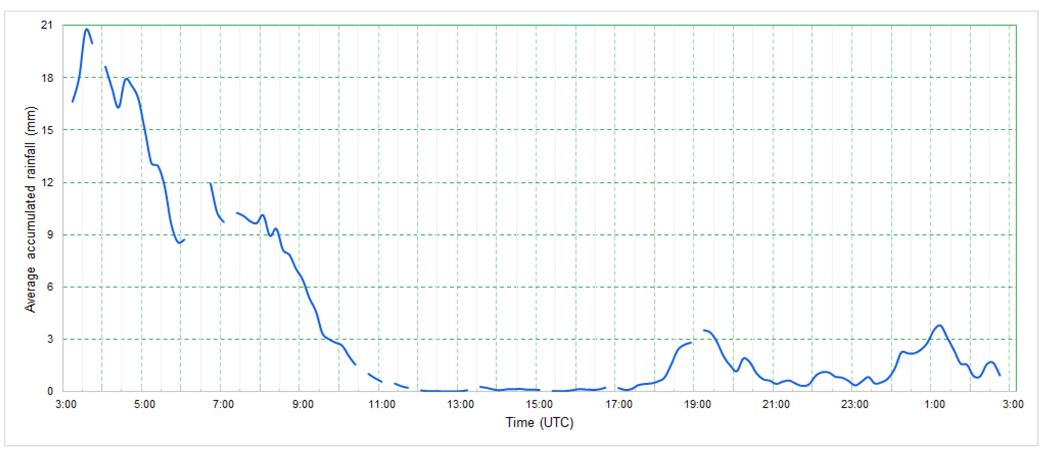
On March 11, 2016, a storm produced the largest flood peak in the city of São Paulo during the observation period. As noted in Figure 7, the maximum hourly accumulated rainfall occurred between 00:00 HL and 01:00 HL. The maximum 10 min accumulated rainfall was 20.7 mm, and the city registered 175 mmh−1 of a maximum precipitation rate. Like many urban flash floods in the city, this event was associated with a passage of a surface cold front associated with the South Atlantic Convergence Zone (SACZ), which usually show large rain volumes for long periods of time [37,38].
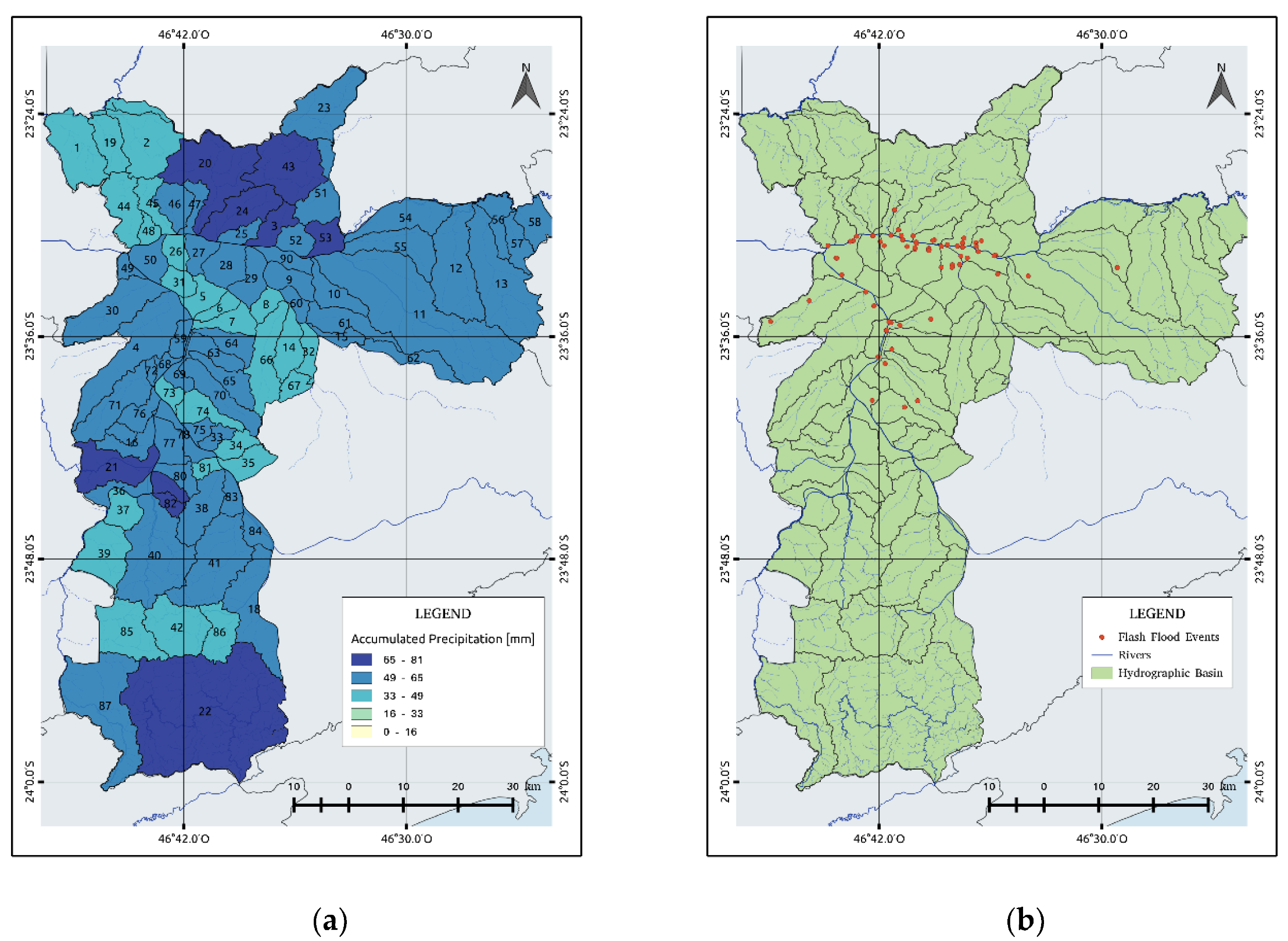
This event produced flash flooding in the city, mainly in the Tietê and Pinheiros rivers overflow, which resulted in several landslides and damaged the city’s infrastructure. The traffic vehicle department of São Paulo observed 93 flooding points around the city. The northern and western zones recorded the highest flash flood rate with 32 flood points, which was followed by the southern, central, eastern, and southeastern zones with 10, 9, 7, and 3 flood points, respectively. Figure 8a shows the 24-h accumulated rainfall on 11 March 2016. The dark areas represent the watersheds that registered up to 65 to 81 mm of accumulated rainfall. Figure 8b shows the location of the flash flood points in the city. Although a greater accumulated precipitation can be observed in the northern and southern areas, the flash flood events were concentrated near the two main rivers due to different relieving soil types. For example, the bordering watersheds, such as those in the north and south, have a declivity of more than 60%, which contributes to flash floods downstream.
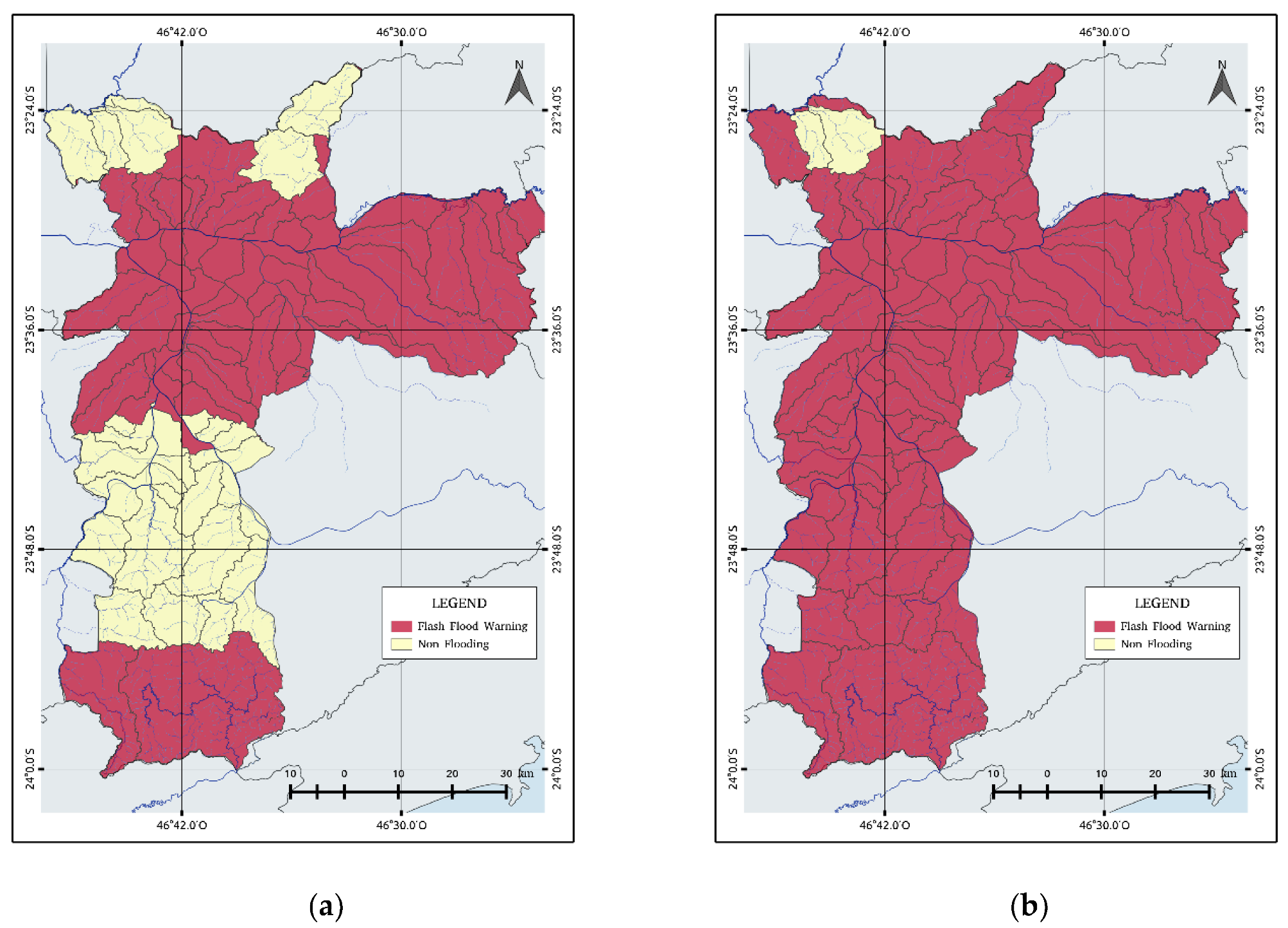
After applying the logistic model, the estimated flash flood warnings were concentrated throughout the city (Figure 9b) with an exception of two watersheds located in the north. From Figure 9a,b, it is possible to compare the flash flood warnings related to the flood points observed on that day and the flash flood forecasting, respectively. The logistic regression model generated false alarms in the southern region and a few cases in the north, mainly in the Tremembé and Anhangüera districts. The predictions have an accuracy of 68% and a mean probability of success of 94%. The computed POD reveals that the logistic regression model improves the predictability of flash floods.
4. Conclusions
In our study, we explored the possibility to develop a methodology to forecast flash flood warnings for each watershed using a binary logistic regression model for the city of São Paulo based on the early 24-h rainfall measurements. The model used rain estimates from the dual-polarization S-band Doppler weather radar (SPOL) from the DAEE and the Technological Center of the Hydraulics Foundation (FCTH). The logistic regression model was adjusted to use 24-h accumulated precipitation, a maximum precipitation rate, and rainfall duration for each watershed.
The model presented a mean POD of 0.459 and a mean FAR of 0.12 for flash flood cases. For non-flash flood cases, the POD was 0.954 and the FAR 0.297. When considering only rainy days, the POD for flash flood cases increases to 0.71. These errors indicate that the developed logistic regression model performs better to predict non-flash flood events.
On average, a higher probability of the occurrence of flash flood events was observed in 48% of the watersheds sampled. These watersheds are located in the eastern and central regions near the Tietê and Pinheiros rivers, and the model showed a POD above 50% and a FAR less than 15%. Moreover, the logistic model showed an 86% accuracy in these regions. These regions also registered greater recurrence of flood points that might influence the accuracy of the model.
In general, the capacity of the binary logistic regression model shows an acceptable probability for flash flood occurrence in a certain number of watersheds, while the probability for non-occurrence of flash flood has a better success rate.
Author Contributions
This study is part of the Masters in Science developed by A.S.V.L., while C.A.M.R. was her advisor. Conceptualization: A.S.V.L. Investigation: A.S.V.L. Supervision: C.A.M.R. Writing, review, and editing, C.A.M.R. All authors have read and agreed to the published version of the manuscript.
Funding
This research was supported by a fellowship from Program PROEX of Coordenação de Aperfeiçoamento de Pessoal de Nivel Superior (CAPES), CAPES Finance Code 001 and Program Pro-Alertas of CAPES (grant number: 88887.091742/2014-01). In addition, one of the authors had support from the Brazilian Research Agency Conselho Nacional de Desenvolvimento Científico e Tecnológico (CNPq) [grant numbers: 483919/2013-6 and 307424/2016-2].
Acknowledgments
The authors acknowledge the Foundation Technological Center of Hydraulics (FCTH) and the Climate Emergency Management Center (CGE) for the data provided in this study.
Conflicts of Interest
The authors declare no conflict of interest.
Appendix A

Table A1.
Logistic regression model coefficients for the three variables included.
| Id | Intercept | Accumulated Precipitation | Maximum Precipitation Rate | Rainfall Duration | Accuracy |
|---|---|---|---|---|---|
| 1 | −3.221 | 0.055 | 0.051 | 0.003 | 0.838 |
| 2 | −21.405 | 139.379 | −143.587 | −2.514 | 0.978 |
| 3 | −3.026 | 0.087 | 0.047 | 0.004 | 0.877 |
| 4 | −3.465 | 0.136 | 0.115 | 0.002 | 0.841 |
| 5 | −3.134 | 0.145 | 0.065 | 0.003 | 0.855 |
| 6 | −3.271 | 0.080 | 0.066 | 0.003 | 0.877 |
| 7 | −3.228 | 0.100 | 0.088 | 0.002 | 0.874 |
| 8 | −2.916 | 0.109 | 0.062 | 0.002 | 0.868 |
| 9 | −3.196 | 0.128 | 0.047 | 0.002 | 0.866 |
| 10 | −3.805 | 0.066 | 0.112 | 0.002 | 0.877 |
| 11 | −3.567 | 0.079 | 0.115 | 0.002 | 0.855 |
| 12 | −3.411 | 0.080 | 0.070 | 0.002 | 0.871 |
| 13 | −3.161 | 0.097 | 0.083 | 0.002 | 0.855 |
| 14 | −3.194 | 0.095 | 0.066 | 0.002 | 0.860 |
| 15 | −3.059 | 0.077 | 0.045 | 0.003 | 0.849 |
| 16 | −3.202 | 0.113 | 0.089 | 0.002 | 0.849 |
| 17 | −3.041 | 0.091 | 0.114 | 0.002 | 0.836 |
| 18 | −2.949 | 0.092 | −0.016 | 0.003 | 0.836 |
Table A2.
Logistic regression model coefficients for the two variables included accumulated precipitation and a maximum precipitation rate.
Table A2.
Logistic regression model coefficients for the two variables included accumulated precipitation and a maximum precipitation rate.
| Id | Intercept | Accumulated Precipitation | Maximum Precipitation Rate | Rainfall Duration | Accuracy |
|---|---|---|---|---|---|
| 19 | −6070 | 0.285 | −0.319 | 0.981 | |
| 20 | −6035 | 0.315 | −0.348 | 0.981 | |
| 21 | −2911 | 0.339 | −0.044 | 0.844 | |
| 22 | −3056 | 0.202 | −0.034 | 0.860 |
Table A3.
Logistic regression model coefficients for the two variables included accumulated precipitation and a maximum precipitation rate.
Table A3.
Logistic regression model coefficients for the two variables included accumulated precipitation and a maximum precipitation rate.
| Id | Intercept | Accumulated Precipitation | Maximum Precipitation Rate | Rainfall Duration | Accuracy |
|---|---|---|---|---|---|
| 23 | −3021 | 0.089 | 0.003 | 0.836 | |
| 24 | −2965 | 0.148 | 0.003 | 0.866 | |
| 25 | −2908 | 0.178 | 0.003 | 0.866 | |
| 26 | −2851 | 0.157 | 0.002 | 0.874 | |
| 27 | −2869 | 0.188 | 0.003 | 0.866 | |
| 28 | −2914 | 0.223 | 0.002 | 0.858 | |
| 29 | −2920 | 0.307 | 0.002 | 0.863 | |
| 30 | −3110 | 0.300 | 0.001 | 0.844 | |
| 31 | −2925 | 0.194 | 0.003 | 0.855 | |
| 32 | −3026 | 0.147 | 0.002 | 0.847 | |
| 33 | −2821 | 0.146 | 0.003 | 0.827 | |
| 34 | −2868 | 0.115 | 0.003 | 0.844 | |
| 35 | −2776 | 0.139 | 0.002 | 0.819 | |
| 36 | −2959 | 0.212 | 0.002 | 0.847 | |
| 37 | −2848 | 0.216 | 0.003 | 0.847 | |
| 38 | −3963 | 0.069 | 0.002 | 0.890 | |
| 39 | −2777 | 0.185 | 0.003 | 0.836 | |
| 40 | −3097 | 0.112 | 0.002 | 0.852 | |
| 41 | −3382 | 0.082 | 0.003 | 0.855 | |
| 42 | −2846 | 0.058 | 0.003 | 0.838 |
Table A4.
Logistic regression model coefficients for the two variables included a maximum precipitation rate and rainfall duration.
Table A4.
Logistic regression model coefficients for the two variables included a maximum precipitation rate and rainfall duration.
| Id | Intercept | Accumulated Precipitation | Maximum Precipitation Rate | Rainfall Duration | Accuracy |
|---|---|---|---|---|---|
| 43 | −3952 | 0.101 | 0.003 | 0.852 | |
| 44 | −3188 | 0.129 | 0.003 | 0.847 | |
| 45 | −3089 | 0.108 | 0.003 | 0.860 | |
| 46 | −3139 | 0.110 | 0.003 | 0.866 | |
| 47 | −3111 | 0.114 | 0.003 | 0.863 | |
| 48 | −2987 | 0.103 | 0.003 | 0.866 | |
| 49 | −2984 | 0.087 | 0.004 | 0.833 | |
| 50 | −3575 | 0.093 | 0.003 | 0.855 | |
| 51 | −3324 | 0.131 | 0.004 | 0.874 | |
| 52 | −3110 | 0.100 | 0.005 | 0.874 | |
| 53 | −3182 | 0.108 | 0.005 | 0.877 | |
| 54 | −3394 | 0.162 | 0.004 | 0.855 | |
| 55 | −3523 | 0.144 | 0.003 | 0.863 | |
| 56 | −3373 | 0.103 | 0.004 | 0.844 | |
| 57 | −3793 | 0.069 | 0.003 | 0.863 | |
| 58 | −3505 | 0.106 | 0.004 | 0.847 | |
| 59 | −3424 | 0.187 | 0.004 | 0.841 | |
| 60 | −3863 | 0.092 | 0.003 | 0.868 | |
| 61 | −4135 | 0.072 | 0.003 | 0.871 | |
| 62 | −3838 | 0.102 | 0.003 | 0.860 | |
| 63 | −3391 | 0.158 | 0.004 | 0.855 | |
| 64 | −3595 | 0.129 | 0.003 | 0.874 | |
| 65 | −4303 | 0.088 | 0.003 | 0.863 | |
| 66 | −3505 | 0.134 | 0.003 | 0.871 | |
| 67 | −3338 | 0.106 | 0.003 | 0.852 | |
| 68 | −3464 | 0.093 | 0.004 | 0.855 | |
| 69 | −3349 | 0.145 | 0.003 | 0.836 | |
| 70 | −3814 | 0.104 | 0.003 | 0.849 | |
| 71 | −3890 | 0.083 | 0.003 | 0.874 | |
| 72 | −3163 | 0.122 | 0.003 | 0.858 | |
| 73 | −3529 | 0.086 | 0.003 | 0.858 | |
| 74 | −3191 | 0.118 | 0.003 | 0.844 | |
| 75 | −3027 | 0.104 | 0.004 | 0.852 | |
| 76 | −3341 | 0.146 | 0.004 | 0.833 | |
| 77 | −3484 | 0.081 | 0.003 | 0.885 | |
| 78 | −3566 | 0.102 | 0.003 | 0.868 | |
| 79 | −3430 | 0.061 | 0.003 | 0.879 | |
| 80 | −3050 | 0.099 | 0.003 | 0.858 | |
| 81 | −2853 | 0.075 | 0.003 | 0.860 | |
| 82 | −3152 | 0.156 | 0.004 | 0.844 | |
| 83 | −3176 | 0.085 | 0.004 | 0.858 | |
| 84 | −3072 | 0.085 | 0.003 | 0.858 | |
| 85 | −2816 | 0.115 | 0.004 | 0.841 | |
| 86 | −3173 | 0.070 | 0.003 | 0.838 | |
| 87 | −3081 | 0.087 | 0.003 | 0.841 | |
| 88 | −31973 | 0.0954 | 0.0028 | 0.8904 | |
| 89 | −31909 | 0.0564 | 0.0035 | 0.8658 |
Table A5.
Logistic regression model coefficients for the one variable included accumulated precipitation.
Table A5.
Logistic regression model coefficients for the one variable included accumulated precipitation.
| Id | Intercept | Accumulated Precipitation | Maximum Precipitation Rate | Rainfall Duration | Accuracy |
|---|---|---|---|---|---|
| 90 | −3.937 | 0.154 | 0.918 |
References
- Munich Re NatCatSERVICE Natural catastrophes in 2019. Available online: https://www.munichre.com/content/dam/munichre/global/content-pieces/documents/munichre-natural-catastrophes-in-2018.pdf/_jcr_content/renditions/original./munichre-natural-catastrophes-in-2018.pdf (accessed on 2 March 2020).
- Muñoz, P.; Orellana-Alvear, J.; Willems, P.; Célleri, R. Flash-Flood Forecasting in an Andean Mountain Catchment-Development of a Step-Wise Methodology based on the Random Forest Algorithm. Water 2018, 10, 1519. [Google Scholar] [CrossRef] [Green Version]
- Chen, M.; Pang, J.; Wu, P. Flood routing model with particle filter-based data assimilation for flash flood forecasting in the micro-model of Lower Yellow River, China. Water 2018, 10, 1612. [Google Scholar] [CrossRef] [Green Version]
- Barros, M.T.L.; Gonçalves, F.M. Meteorological radar and flood forecasting. In Proceedings of the 31st Conference on Radar Meteorology, Seattle, WA, USA, 6–12 August 2003; pp. 1–5. [Google Scholar]
- Oliveira, C.P.M.; da Silva, C.V.; Sosnoski, A.S.K.B.; Bozzini, P.L.; Rossi, D.M.; Uemura, S.; Conde, F. Warning System Based on Real-Time Flood Forecasts in São Paulo, Brazil. In Proceedings of the 6th International Conference on Flood Management, São Paulo, Brazil, 16–18 September 2014; pp. 1–12. [Google Scholar]
- Corral, C.; Berenguer, M.; Sempere-Torres, D.; Poletti, L.; Silvestro, F.; Rebora, N. Comparison of two early warning systems for regional flash flood hazard forecasting. J. Hydrol. 2019, 572, 603–619. [Google Scholar] [CrossRef] [Green Version]
- Xia, X.; Liang, Q.; Ming, X.; Hou, J. An efficient and stable hydrodynamic model with novel source term discretization schemes for overland flow and flood simulations. Water Resour. Res. 2017, 53, 3730–3759. [Google Scholar] [CrossRef]
- Fiorentino, M.; Manfreda, S.; Iacobellis, V. Peak runoff contributing area as hydrological signature of the probability distribution of floods. Adv. Water Resour. 2007, 30, 2123–2134. [Google Scholar] [CrossRef]
- Alfieri, L.; Burek, P.; Dutra, E.; Krzeminski, B.; Muraro, D.; Thielen, J.; Pappenberger, F. GloFAS-global ensemble streamflow forecasting and flood early warning. Hydrol. Earth Syst. Sci. 2013, 17, 1161–1175. [Google Scholar] [CrossRef] [Green Version]
- Kulkarni, A.T.; Eldho, T.I.; Rao, E.P.; Mohan, B.K. An integrated flood inundation model for coastal urban watershed of Navi Mumbai, India. Nat. Hazards 2014, 73, 403–425. [Google Scholar] [CrossRef]
- Lohmann, M. Regressão Logística E Redes Neurais Aplicadas À Previsão Probabilística De Alagamentos No Município De Curitiba, Pr. Ph.D. Thesis, Universidade Federal do Paraná, Curitiba, Brazil, 2011. [Google Scholar]
- Sahoo, G.B.; Ray, C.; De Carlo, E.H. Use of neural network to predict flash flood and attendant water qualities of a mountainous stream on Oahu, Hawaii. J. Hydrol. 2006, 327, 525–538. [Google Scholar] [CrossRef]
- Chang, F.-J.; Chen, P.-A.; Lu, Y.-R.; Huang, E.; Chang, K.-Y. Real-time multi-step-ahead water level forecasting by recurrent neural networks for urban flood control. J. Hydrol. 2014, 517, 836–846. [Google Scholar] [CrossRef]
- Chiang, Y.M.; Hao, R.N.; Zhang, J.Q.; Lin, Y.T.; Tsai, W.P. Identifying the sensitivity of ensemble streamflow prediction by artificial intelligence. Water 2018, 10, 1341. [Google Scholar] [CrossRef] [Green Version]
- Wu, J.; Liu, H.; Wei, G.; Song, T.; Zhang, C.; Zhou, H. Flash flood forecasting using support vector regression model in a small mountainous catchment. Water 2019, 11, 1327. [Google Scholar] [CrossRef] [Green Version]
- Bui, D.T.; Khosravi, K.; Li, S.; Shahabi, H.; Panahi, M.; Singh, V.P.; Chapi, K.; Shirzadi, A.; Panahi, S.; Chen, W.; et al. New hybrids of ANFIS with several optimization algorithms for flood susceptibility modeling. Water 2018, 10, 1210. [Google Scholar]
- Wang, Z.; Lai, C.; Chen, X.; Yang, B.; Zhao, S.; Bai, X. Flood hazard risk assessment model based on random forest. J. Hydrol. 2015, 527, 1130–1141. [Google Scholar] [CrossRef]
- Mosavi, A.; Ozturk, P.; Chau, K.W. Flood prediction using machine learning models: Literature review. Water 2018, 10, 1536. [Google Scholar] [CrossRef] [Green Version]
- Albers, S.J.; Déry, S.J.; Petticrew, E.L. Flooding in the Nechako River Basin of Canada: A random forest modeling approach to flood analysis in a regulated reservoir system. Can. Water Resour. J. 2016, 41, 250–260. [Google Scholar] [CrossRef]
- Chau, K.T.; Chan, J.E. Regional bias of landslide data in generating susceptibility maps using logistic regression: Case of Hong Kong Island. Landslides 2005, 2, 280–290. [Google Scholar] [CrossRef]
- Rasyid, A.R.; Bhandary, N.P.; Yatabe, R. Performance of frequency ratio and logistic regression model in creating GIS based landslides susceptibility map at Lompobattang Mountain, Indonesia. Geoenviron. Disasters 2016, 3, 19. [Google Scholar] [CrossRef] [Green Version]
- Sánchez, J.L.; Marcos, J.L.; de la Fuente, M.T.; Castro, A. A logistic regression model applied to short term forecast of hail risk. Phys. Chem. Earth 1998, 23, 645–648. [Google Scholar] [CrossRef]
- Gascón, E.; Merino, A.; Sánchez, J.L.; Fernández-González, S.; García-Ortega, E.; López, L.; Hermida, L. Spatial distribution of thermodynamic conditions of severe storms in southwestern Europe. Atmos. Res. 2015, 164–165, 194–209. [Google Scholar] [CrossRef]
- Barros, M.T.L.; Conde, F. Urban Flood Warning System Social Benefits. In Proceedings of the World Environmental and Water Resources Congress 2017, Sacramento, CA, USA, 21–25 May 2017; pp. 12–23. [Google Scholar]
- Sosnoski, A.S.K.B.; Pion, S.M.; Uemura, S.; Conde, F. Calibração e Validação de modelo de previsão de inundações em tempo real do Município de São Paulo. In Proceedings of the XXI Simposio Brasileiro de Recursos Hidricos, Brasília-DF, Brazil, 22–27 November 2015; pp. 1–8. [Google Scholar]
- Pereira Filho, A.J.; Haas, R.; Ambrizzi, T. Caracterização de eventos de enchente na Bacia do Alto Tietê por meio do radar meteorológico e da modelagem numérica de mesoescala. In Proceedings of the Congresso Brasileiro de Meteorologia, Foz do Iguaçu, Brazil, 4–9 August 2002; pp. 2864–2873. [Google Scholar]
- Barros, M.T.L.; Pion, H.A.; Gonçalves, F.M. Flood Warning Model for Sao Paulo City. Urban Drainage Modeling. Available online: https://ascelibrary.org/doi/abs/10.1061/40583(275)31 (accessed on 10 February 2020).
- Ryzhkov, A.V.; Schuur, T.J.; Burgess, D.W.; Heinselman, P.L.; Giangrande, S.E.; Zrnic, D.S. The joint polarization experiment: Polarimetric rainfall measurements and hydrometeor classification. Bull. Am. Meteorol. Soc. 2005, 86, 809–824. [Google Scholar] [CrossRef] [Green Version]
- SELEX Manual. Rainbow 5. Products and Algorithms; Selex SI GmbH: Neuss, Germany, 2010; pp. 113–124. [Google Scholar]
- Viteri, L.A. Caracterização da chuva estimada pelo radar durante eventos de alagamento na cidade de São Paulo. Master’s Thesis, Universidade de São Paulo, São Paulo, Brazil, 2018. [Google Scholar]
- Ministério de Integração Nacional; Secretaria Nacional de Defesa Civil; Centro Nacional de Gerenciamento de Riscos e Desastres. Anuário Brasileiro De Desastres Naturais; CENAD: Brasília, Brazil, 2014. [Google Scholar]
- Cox, D.R. The Regression Analysis of Binary Sequences. J. R. Stat. Soc. Ser. B 1958, 20, 215–242. [Google Scholar] [CrossRef]
- Raschka, S. Python Machine Learning, 1st ed.; Packt Publishing: Birmingham, UK, 2015. [Google Scholar]
- Pan, W. Akaike’s information criteria in generalized estimating equations. Biometrics 2001, 57, 120–125. [Google Scholar] [CrossRef] [PubMed]
- Donaldson, R.J.; Dyer, R.M.; Kraus, R.M. An objective evaluation of techniques for predicting severe weather events. Preprints. In 9th Conference on Severe Local Storm; Norman, Org.; American Meteorological Society: Boston, MA, USA, 1975; pp. 321–326. [Google Scholar]
- Wilks, D.S. Statistical Methods in the Atmospheric Sciences, 3rd ed.; Academic Press: Waltham, MA, USA, 2011. [Google Scholar]
- Oliveira, R.A.; Braga, R.C.; Vila, D.A.; Morales, C.A. Evaluation of GPROF-SSMI/S rainfall estimates over land during the Brazilian CHUVA-VALE campaign. Atmos. Res. 2015, 163, 102–116. [Google Scholar] [CrossRef]
- Satyamurty, P.; Sousa, S.B., Jr.; De Teixeira, M.D.S.; Silva, L.E.M.G. Da Regional circulation differences between a rainy episode and a nonrainy episode in eastern São Paulo State in March 2006. Rev. Bras. Meteorol. 2008, 23, 404–416. [Google Scholar] [CrossRef]
Figure 1.
Location map of the study area and the position of S-band Doppler weather radar (SPOL) radar over the Sao Paulo Metropolitan Region.
Figure 1.
Location map of the study area and the position of S-band Doppler weather radar (SPOL) radar over the Sao Paulo Metropolitan Region.

Figure 2.
Total number of flash flood warning sites in Sao Paulo city.

Figure 3.
Architecture of a logistic regression model.

Figure 4.
Methodological flowchart used in the binary logistic regression model.

Figure 5.
Location Basins map. The letters A (Accumulated precipitation), B (Maximum Precipitation Rate), and C (Rainfall Duration) represent the predictor variables.
Figure 5.
Location Basins map. The letters A (Accumulated precipitation), B (Maximum Precipitation Rate), and C (Rainfall Duration) represent the predictor variables.

Figure 6.
Spatial distribution of performance metrics, which include the probability of detection (POD) and false alarm ratio (FAR), in São Paulo for flash flood and non-flash flood events: (a,b) the POD and FAR of flash flood events, and (c,d) the POD and FAR of non-flash flood events.
Figure 6.
Spatial distribution of performance metrics, which include the probability of detection (POD) and false alarm ratio (FAR), in São Paulo for flash flood and non-flash flood events: (a,b) the POD and FAR of flash flood events, and (c,d) the POD and FAR of non-flash flood events.

Figure 7.
Time series of 10-min accumulated rainfall over São Paulo for 11 March 2016 based on observations from the SPOL weather radar.
Figure 7.
Time series of 10-min accumulated rainfall over São Paulo for 11 March 2016 based on observations from the SPOL weather radar.

Figure 8.
Spatial distributions of (a) 24-h accumulated rainfall on 11 March 2016 and (b) flood points registered on 11 March 2016 by the Climate Emergency Management Center (CGE).
Figure 8.
Spatial distributions of (a) 24-h accumulated rainfall on 11 March 2016 and (b) flood points registered on 11 March 2016 by the Climate Emergency Management Center (CGE).

Figure 9.
Spatial distributions of (a) flash flood warning observations and (b) probability of flash flood warnings using the binary logistic model.
Figure 9.
Spatial distributions of (a) flash flood warning observations and (b) probability of flash flood warnings using the binary logistic model.

Table 1.
Evaluation of logistic regression models for predicting flash floods.
| Variables | N | Akaike Information Criterion (AIC) |
|---|---|---|
| A, B, C | 3 | 56.96 |
| A, B | 2 | 54.99 |
| A, C | 2 | 56.72 |
| B, C | 2 | 55.30 |
| A | 1 | 54.87 |
| B | 1 | 53.35 |
| C | 1 | 53.99 |
A: Accumulated precipitation, B: maximum precipitation rate, and C: rainfall duration.
Table 2.
Average scores calculated for occurrence/non-occurrence flash flood events with unconditional (total) and conditional rainy days.
Table 2.
Average scores calculated for occurrence/non-occurrence flash flood events with unconditional (total) and conditional rainy days.
| Scores | Total | Only Rainy Days | ||
|---|---|---|---|---|
| Occurrence | Non-Occurrence | Occurrence | Non-Occurrence | |
| Accuracy | 0.861 | 0.800 | 0.745 | 0.631 |
| Bias | 0.648 | 1.083 | 0.654 | 1.198 |
| Probability of Detection | 0.459 | 0.954 | 0.709 | 0.891 |
| False Alarm Ratio | 0.119 | 0.297 | 0.254 | 0.291 |
| Critical Success Index | 0.389 | 0.846 | 0.391 | 0.685 |
© 2020 by the authors. Licensee MDPI, Basel, Switzerland. This article is an open access article distributed under the terms and conditions of the Creative Commons Attribution (CC BY) license (http://creativecommons.org/licenses/by/4.0/).
Share and Cite
MDPI and ACS Style
Viteri López, A.S.; Morales Rodriguez, C.A. Flash Flood Forecasting in São Paulo Using a Binary Logistic Regression Model. Atmosphere 2020, 11, 473. https://doi.org/10.3390/atmos11050473
AMA Style
Viteri López AS, Morales Rodriguez CA. Flash Flood Forecasting in São Paulo Using a Binary Logistic Regression Model. Atmosphere. 2020; 11(5):473. https://doi.org/10.3390/atmos11050473
Chicago/Turabian StyleViteri López, Andrea Salomé, and Carlos Augusto Morales Rodriguez. 2020. "Flash Flood Forecasting in São Paulo Using a Binary Logistic Regression Model" Atmosphere 11, no. 5: 473. https://doi.org/10.3390/atmos11050473
Note that from the first issue of 2016, this journal uses article numbers instead of page numbers. See further details here.