Explosive Cyclogenesis around the Korean Peninsula in May 2016 from a Potential Vorticity Perspective: Case Study and Numerical Simulations


1
Marine Disaster Research Center, Korea Institute of Ocean Science & Technology, Busan 49111, Korea
2
Center for Climate Physics, Institute for Basic Sciences, Busan 34126, Korea
3
Department of Atmospheric Sciences, Pusan National University, Busan 46241, Korea
4
Department of Civil Engineering, Kangwon National University, Samcheok 25913, Korea
*
Author to whom correspondence should be addressed.
Atmosphere 2019, 10(6), 322; https://doi.org/10.3390/atmos10060322
Submission received: 23 April 2019
/
Revised: 3 June 2019
/
Accepted: 4 June 2019
/
Published: 12 June 2019
(This article belongs to the Special Issue Weather and Climate Extremes: Current Developments)
Abstract
:An explosive cyclone event that occurred near the Korean Peninsula in early May 2016 is simulated using the Weather Research and Forecasting (WRF) model to examine the developmental mechanisms of the explosive cyclone. After confirming that the WRF model reproduces the synoptic environments and main features of the event well, the favorable environmental conditions for the rapid development of the cyclone are analyzed, and the explosive development mechanisms of the cyclone are investigated with perturbation potential vorticity (PV) fields. The piecewise PV inversion method is used to identify the dynamically relevant meteorological fields associated with each perturbation PV anomaly. The rapid deepening of the surface cyclone was influenced by both adiabatic (an upper tropospheric PV anomaly) and diabatic (a low-level PV anomaly associated with condensational heating) processes, while the baroclinic processes in the lower troposphere had the smallest contribution. In the explosive phase of the cyclone life cycle, the diabatically generated PV anomalies associated with condensational heating induced by the ascending air in the warm conveyor belt are the most important factors for the initial intensity of the cyclone. The upper-level forcing is the most important factor in the evolution of the cyclone’s track, but it is of secondary importance for the initial strong deepening.
1. Introduction
Explosive cyclones are extratropical cyclones characterized by a strong deepening (a sea level pressure decrease larger than 24 hPa within 24 h at 60° N or the equivalent [1]) and are often linked not only to extreme weather conditions, including strong winds and heavy rainfall, but also to extreme ocean events such as abnormally high waves [2] and, in some cases, storm surge. Sanders and Gyakum [1] first conducted a study on explosive cyclones in 1980 and demonstrated the importance of the baroclinic instability to this phenomenon; since then, many researchers have identified the development mechanisms of explosive cyclones, including physical and dynamical processes [3,4,5,6,7,8,9,10].
According to Shapiro et al. [11], explosive cyclones initially develop in response to a combination of different mechanisms that include upper-level cyclonic vorticity advection, low-level warm air advection, and latent heat release. This may be influenced by Rossby wave breaking, which contributes to the development of intense cyclones by constraining and intensifying the upper-level jet stream [12,13,14]. Furthermore, the heating and moistening of the atmosphere and the reduced stability due to air–sea interactions are also important prior to and during explosive cyclone development [15,16,17]. A moisture flux accompanied by the onshore flow associated with a lower-tropospheric potential vorticity maximum contributes to latent heating in the cyclones [18], which may strengthen the cyclones through the influence of the enhanced latent heat release (LHR) in the warm conveyor belt (WCB) [19,20,21,22,23,24]. According to Fosdick and Smith [25], LHR can significantly contribute to explosive cyclone development by reinforcing the development and propagation influence of other forcing mechanisms. Heo et al. [5] found that LHR contributes to approximately half of the intensification during the initial stage of explosive cyclone development. Schemm and Wernli [22] described how the LHR embedded in the WCB intensifies the upper- and low-level potential vorticity (PV) anomalies in an idealized extratropical cyclone and how the two PV anomalies accelerate the near-surface wind speed (low-level PV anomaly) as well as the upper-level jet stream and downstream development (upper-level PV anomaly). The impact on the deepening was later confirmed via climatological analysis by Binder et al. [23].
Explosive cyclone development is usually initiated by upper-level PV anomalies interacting with strong surface baroclinicity [26,27], but it is greatly enhanced by deep moisture convection and strong latent and sensible heat fluxes from the ocean [28,29]. More recently, many studies have been conducted to identify the relative importance of each physical process. Sensitivity studies have commonly been used to investigate the importance of various processes on explosive cyclone development [5,26,30]. Such sensitivity studies have inherent limitations in interpreting the nonlinearity of physical interactions. However, the piecewise PV inversion (PPVI) method developed by Davis and Emanuel [31] is able to provide the relative importance of various physical processes in explosive cyclone development. The effects of discrete PV anomalies during this process can be clearly demonstrated in PPVI results because the PPVI method allows for the recovery of the balanced horizontal wind field and temperature fields attributable to a discrete PV anomaly [32].
Yoshida and Asuma [33] showed that the explosive cyclones over the northwestern Pacific region formed over land and ocean, but the maximum deepening almost always occurred over the ocean at latitudes greater than 35° N. Recent studies have shown the relative importance of upper-level forcing, latent heating, and surface heat fluxes in developing explosive cyclones over East Asian marginal seas during the cold season [34,35]. However, an explosive cyclone formed and developed over land in the northern part of the Korean Peninsula in May 2016, resulting in high winds and waves impacting the east coast of Korea. The cyclone was characterized by extraordinarily rapid development; hence, this study aims to better understand its characteristics and examine its development mechanisms.
To obtain a better understanding of explosive cyclone development, we analyze numerical simulations performed with the Weather Research and Forecasting (WRF) model by employing the PPVI method to examine the relative influences of the upper tropospheric, lower tropospheric, and diabatic PV anomalies in the explosive cyclone intensification phase. We describe the development on the basis of synoptic surface data and satellite images and examine information related to the data, model, methodology, and experimental design in Section 2. Section 3 presents the results of the numerical experiments and the processes believed to play a critical role in explosive cyclogenesis. Concluding remarks are provided in Section 4.
2. Materials and Methods
2.1. Explosive Cyclone Overview
The explosive cyclone initially formed in the eastern part of China with a central sea level pressure (CSLP) of 1003 hPa at 0000 UTC on 2 May 2016 (Figure 1). It moved north-eastward and intensified at 0000 UTC on 18 May near 35° N/118° E with a CSLP of 1001 hPa and a maximum surface wind speed (MSW) of 4 m s−1. During the subsequent 24 h beginning at 0600 UTC on 2 May, the northeastward-moving cyclone developed at a CSLP-deepening rate of 24 hPa (24 h)−1, and an MSW of ~35 m s−1 appeared at 0600 UTC on 3 May. This period is defined as the developing stage. As the explosive cyclone rapidly developed beginning at 0000 UTC on 3 April, it began to affect the coastal areas, and large waves were caused by the strong winds accompanying the cyclone. The observed maximum wave heights and periods over the East/Japan Sea were 7.2 m and 9.1 s at Ulsan (35.6° N, 129.3° E), 9.3 m and 9.1 s at Uljin (36.9° N, 129.4° E), and 8.5 m and 9.1 s at the Donghae buoy (37.5° N, 130.0° E) on 3 May. Despite slight increases, the minimum CSLP was maintained for 12 h. Thus, this period between 0600 UTC and 1800 UTC on 3 May is defined as the mature stage. The cyclone center began to weaken after 0000 UTC on 4 May, and it dissipated at 0000 UTC on 5 May 2016. This period is defined as the decaying stage.
Figure 2 shows a Communication, Ocean and Meteorological Satellite 1 (COMS-1) infrared (IR) satellite image from 1200 UTC on 2 May to 0000 UTC on 4 May 2016. The cyclogenesis seen in Figure 2a shows one large area covered by clouds over the east coast of China and the Yellow Sea. A dark feature in the water vapor (WV) image indicating a dry slot in Figure 2b appeared in the upper left quadrant of the initial cyclone. The cloudy area associated with the cyclone enlarged and moved eastwards at 0000 UTC on 3 May (Figure 2c). At this time, the WV image in Figure 2d shows a cloud band curling around the cyclone center and a dry intrusion forming a hook-shaped cloud pattern, which indicates explosive cyclogenesis [36]. The hook-shaped cloud developed into a spiral cloud, which is characteristic of the mature stage of an explosive cyclone (Figure 2e). Strong winds reaching the surface in the dry air ahead of the hook-shaped cloud head can be produced by a sting jet, which is also present at that time, with the WCB located beneath the PV intrusion [37,38]. The dry intrusion enters the circulation of the surface cyclone, which means that cold, dry air with a high PV intrudes into the lower troposphere from the lower stratosphere and/or upper troposphere. The spiral cloud pattern was associated with the dry intrusion from the upper level and indicates the condition of the upper-level cyclonic circulation (Figure 2f). From synoptic charts, the dry intrusion with a cloudless area is found to descend over the warm and moist sectors, which can lead to potential instability. The spiral patterns developed after the surface deepening had nearly finished, and the upper-level cyclone continued to intensify or maintain its strength.
2.2. Data
The following data are employed herein: (1) the analyzed surface weather charts and upper-level weather charts from the Korean Meteorological Administration (KMA) for cyclone tracking, (2) the COMS-1 infrared imagery downloaded from the satellite information service system of the KMA, and (3) the global final analysis (FNL) dataset produced with a resolution of 1.0° and 26 vertical levels for numerical simulations and experiments, which are provided by the National Centers for Environmental Prediction (NCEP) and the National Center for Atmospheric Research (NCAR). The NCEP FNL is taken as the initial and 6-hourly forecast files for the initial and boundary conditions.
2.3. Model Description
To obtain a comprehensive three-dimensional structure of the explosive cyclone, the Advanced Research WRF (WRF-ARW) model [39] version 3.7 developed by NCAR was used. The model incorporates fully incompressible nonhydrostatic equations in conjunction with terrain-following vertical coordinates. The model was run with two domains starting at 0000 UTC 2 May 2016 and integrated for 72 h to include the entire lifetime of the explosive cyclone. The horizontal resolutions of the outer and inner domains are 20 and 4 km with 218 × 218 and 361 × 361 grids (Figure 3), respectively. Both domains have 40 vertical layers from the surface to the 50 hPa level, and the model instantaneous outputs were saved every hour. The Yonsei University (YSU) planetary boundary layer scheme [40], Noah Land Surface Model [41], Kain–Fritsch cumulus parameterization scheme [42], Dudhia short-wave and rapid radiative transfer model (RRTM) long-wave radiation scheme [43], and the WRF Single-Moment 6-Class Microphysics Scheme [44] were applied to both simulations. A summary of the model configuration parameters and physical schemes used is given in Table 1.
2.4. Piecewise PV Analysis
The Ertel PV (EPV) is defined as [45,46]
where ρ is the density, η is the absolute vorticity vector, and θ is the potential temperature. The PV is expressed in PV units (PVU; 1 PVU = 10−6 m2 s−1 K kg−1). The EPV is conserved for the primitive equations given an adiabatic frictionless flow. Considering a given distribution of the PV throughout a domain, an appropriate balance condition, and suitable boundary conditions, the PPVI allows for the recovery of the mass and momentum fields attributable to discrete PV anomalies. The Davis and Emanuel [31] method, which is used in this study, assumes (1) hydrostatic balance and (2) that the magnitude of the irrotational component of the wind is much smaller than the magnitude of the nondivergent component (i.e., ). Applying these approximations, the divergence equation and Equation (1) can be rewritten as
where Φ is the geopotential, ψ is the nondivergent stream function, λ is the longitude, ϕ is the latitude, a is the radius of the earth, P is the pressure, and is the Exner function, which serves as the vertical coordinate. Equation (2) is a nonlinear balance equation by Charney [47], which has been demonstrated by previous studies to be an excellent approximation to observed flows [48], thus validating the application of PV diagnostics to the real atmosphere [49].
2.5. Experimental Design
To quantify the impact of various PV anomalies, including the upper-level trough, the stratospheric air intrusion, the LHR, the sensible heat flux, and the enhanced local baroclinicity from differential diabatic heating on the explosive cyclogenesis, PPVI was conducted. PPVI has been discussed in detail by the authors of previous studies [31,50,51,52]. In order to use the PPVI method effectively, it is necessary to meaningfully partition the perturbation PV [51]. In order to invert particular PV anomalies, a mean state must be defined. The mean state for the present case is defined as the time average between 0000 UTC 1 May and 0000 UTC 6 May 2016. Given the mean state, the whole atmosphere was partitioned into four parts in a domain (10–60° N, 90–170° E) according to same approach in Baxter et al. [53]: (1) the upper-level perturbation PV (UP): this anomaly represents the main upper-level forcing and is defined as all of the positive and negative perturbation PVs with an relative humidity (RH) < 70% from 500 hPa to the 100 hPa boundary PV; (2) the moist interior PV (MP): the lower-tropospheric PV anomaly related to condensational heating is defined as all positive perturbation PVs with an RH ≥ 70% from 950 hPa to 400 hPa; (3) the lower boundary (LP): this anomaly represents the low-level baroclinicity and is defined as all positive and negative perturbation PVs from the surface through 925 hPa; and (4) the remaining interior PV (RP): all positive and negative perturbation PVs with an RH < 70% from 950 hPa to 550 hPa, which are likely remnants of the diabatically generated PV. The removal of the UP and MP simulations was designed to isolate the effect of the tropopause undulations associated with upper-tropospheric/lower-stratospheric air and to consider the effect of condensation-related diabatic processes, respectively. The removal of the LP simulation was designed to consider the effect of diabatic heating that was closely related to the baroclinicity and boundary layer processes. The removal of the RP simulation was designed to examine the effect of the diabatically generated PV remnants not included in the above three simulations. To illustrate the effect of the removal of the four partitioned perturbation PVs, four simulations were performed—namely, the removal of UP (RUP), MP (RMP), LP (RLP), and RP (RRP). Figure 4 shows the initial conditions of each simulation for a 500 hPa geopotential height and the sea level pressure after the PPVI procedure. Finally, to gain an accurate understanding of the impacts of the upper-level perturbation PV and moist interior PV on cyclogenesis, two additional simulations were performed, in which UP and MP are doubled; they are denoted as DUP and DMP, respectively.
3. Results and Discussion
3.1. Control Simulation
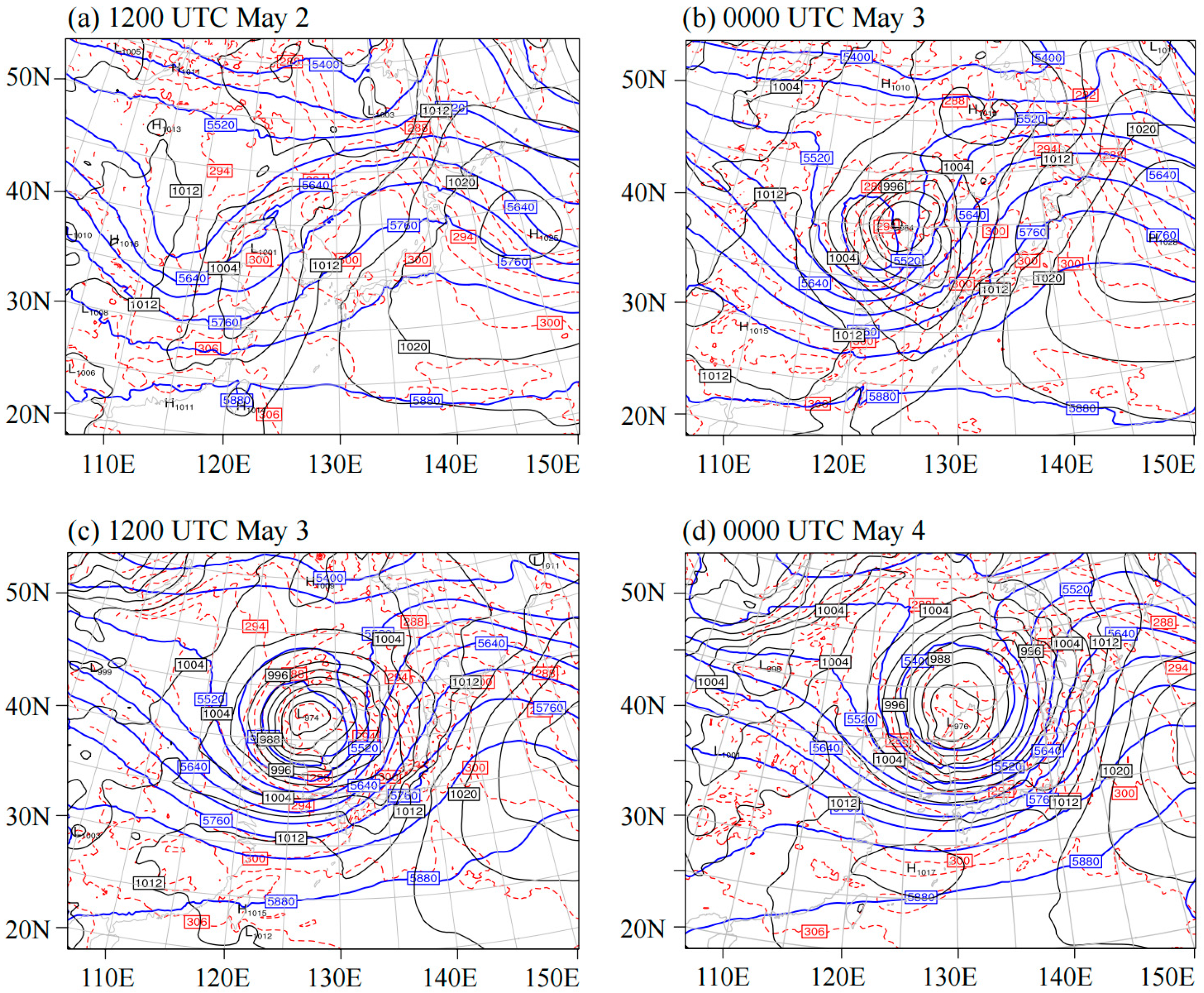
At 1200 UTC on 2 May, the flow was characterized by a short-wave trough feature at the 500 hPa level near 37° N, 113° E. The trough moved northeastward and deepened during the following 24 h. The initial surface cyclone with a CSLP of 1002 hPa formed within a strong baroclinic zone southeast of a short-wave trough aloft (Figure 5a). The short-wave trough with its positively tilted axis over the area east of China is evident at the 500 hPa level. The 500 hPa short-wave trough was located ~10° longitude upstream from the surface cyclone, which was characterized with a strong isotherm gradient and strong baroclinicity. This superposition between the surface cyclone and the short-wave trough provides a favorable condition for the surface cyclone to develop. At 0000 UTC on 3 May, the surface cyclone rapidly deepened to a CSLP of 982 hPa and moved northeastward to the northern part of the Korean Peninsula (Figure 5b). The 850 hPa potential temperature contour and the 500 hPa isohypse at the leading edge of the trough intersect, suggesting that baroclinicity and warm air advection are intensifying over the region. The warm sector in the WCB’s region of strongest ascent was linked with the upper-level PV anomaly. Then, the 500 hPa short-wave trough developed into a cut-off low. A very strong upper-level jet is located at the base of the cut-off, reaching a value of ~45 m s−1. During the following 12 h, the surface cyclone reached its maximum intensity with a CSLP of 972 hPa (Figure 5c). Warm advection enhanced the 500 hPa ridge, and cold advection deepened the 500 hPa trough, which shows a well-developed baroclinic pattern. At 0000 UTC on 4 May, the surface cyclone remained almost stationary with a CSLP of 974 hPa. The system showed evidence of occlusion because the temperature advection weakened and completely lost its vertical tilt (Figure 5d). Although there are slight differences in the position between the observed and model-simulated explosive cyclone from its initial to final stages, the simulation results of the WRF model can be used to examine the development mechanisms of the explosive cyclone.
The evolution of the PV on the 320-K isentropic surface from 1200 UTC 2 May to 0000 UTC 4 May is given in Figure 5 to show the necessary conditions for cyclogenesis. At 1200 UTC 2 May, a southward penetration of the PV contours was simulated at approximately 35° N, 113° E, with a local maximum of PV greater than 7.0 PVU directly above the positively tilted trough at the 500 hPa level (Figure 6a). During the following 12 h, the PV anomaly core moved northeastward over the Shandong Peninsula near 36° N, 122° E (Figure 6b), while the cut-off low was generated by the deepening of the 500 hPa trough. This was because the negative PV anomaly over the surface cyclone was intensified by cloud diabatic processes in the WCB outflow region and the southern part of the high-PV air stream cut off from the main stratospheric PV reservoir [22,23], as shown in Figure 5b. Then, intense condensational heating and low-level PV production were induced by the ascending air in the WCB. At 1200 UTC 3 May, the PV anomaly core on the 320 K isentropic surface was located very close to the surface cyclone center. A cyclonic rolling-up of the 300 hPa PV anomaly exceeding 5.0 PVU was generated around the center of the surface cyclone, developing the characteristic inverted comma shape that is associated with the lowermost stratospheric dry air intrusion (Figure 6c). The upper-level PV anomaly and the comma-shaped cloud shown in Figure 2e,f were closely associated with the dry air intrusion to the rear of the surface cyclone.
For a better analysis of the three-dimensional aspects of the PV evolution, Figure 7 shows the vertical cross section of the simulated PV from 1200 UTC 2 May to 1200 UTC 4 May along a longitudinal line based on the position of the surface cyclone center. As a result of the gradual tropopause intrusion, the high PV tongue descended from the upper troposphere to the middle troposphere with the 1.6-PVU contour extending downward to the lowest point of 500 hPa at 1200 UTC on 2 May 2016 (Figure 7a). Meanwhile, there were two lower-level high PVs, one between 500 and 700 hPa and the other between 800 and 900 hPa. This shows that a PV tower is beginning to form through a connection between the upper-level high PVs and lower-level high PVs. At 0000 UTC on 3 May (Figure 7b), the PV tower formed corresponding to the time at which the surface cyclone reached its deepest intensity. It is noted that the increase and upward extension of the lower-level PV reached up to 2.7 PVU, occurring between 500 and 900 hPa, and the upper-level PV moved eastward to the region of enhanced low-level PV ~12 h before the formation of the PV tower. The amplification of the explosive cyclone resulted from the interaction between the upper- and lower-level PV anomalies, inducing strong cyclonic circulation from the surface to the tropopause (Figure 7c). This result is in agreement with the findings in previous studies [15,16,54], which showed the importance of the interaction between the upper-level PV anomalies and the diabatically induced low-level PV anomalies. Therefore, explosive cyclogenesis can be regarded as a result of the PV tower that forms through both adiabatic (upper-level PV) and diabatic (lower-level PV) processes.
3.2. PPVI Results
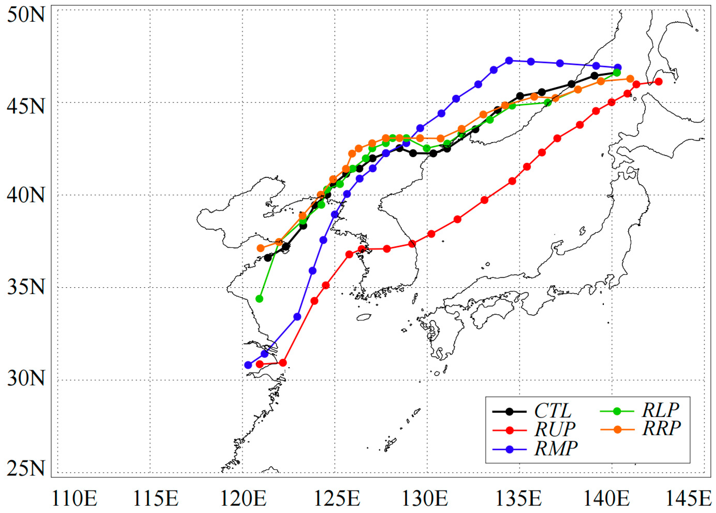
The effects of each of the four perturbation PVs on the CSLP changes during the lifecycle of the explosive cyclone are presented. Figure 8 shows the time series of the CSLP simulated using the initial and boundary conditions from each of the simulations of RUP, RMP, RLP, and RRP during the 36-h period from 1200 UTC 2 May to 0000 UTC 4 May 2016. Compared to other simulations, the RUP and RMP simulations produced apparently weak cyclones (Figure 8a), which clearly shows the reduced influence of the upper-level and moist interior PV anomalies on the surface cyclogenesis. The RUP cyclone continued to deepen with a small deepening rate throughout the 48-h simulation, although the initial CSLP was smaller than that of the RMP cyclone. The RMP simulation is similar in deepening rate to the control (CTL) simulation during a +27-h integration (Figure 8b), but it has a weak cyclone because the highest initial CSLP is 1019 hPa. Nevertheless, the RMP cyclone also rapidly developed with a deepening of 27 hPa during the first 24-h integration. Thus, the RMP cyclone develops a 16 hPa weaker CSLP by the 30-h integration, although it begins with a 15 hPa weaker CSLP than that of the CTL. This result implies that the lower-tropospheric PV anomalies associated with condensational heating between 400 and 950 hPa have a greater impact on the initial cyclogenesis. In addition, the upper-level PV anomaly is an important factor in both the initial cyclogenesis and the development of the cyclone throughout the cyclone’s lifecycle. Figure 8a also shows that the time variation in the simulated CSLP of RRP is almost equal to that in the CTL throughout the lifecycle. The CSLPs in all simulations represent the maximum intensities of the cyclone: 973.3 hPa at +27 h in the CTL, 992.7 hPa at +45 h in RUP, 984.9 hPa at +30 h in RMP, 973.3 hPa at +30 h in RLP, and 971.7 hPa at +27 h in RRP. Figure 9 shows the cyclone tracks represented by the locations of the CSLP minima simulated using the initial and boundary conditions from each of the four perturbation PVs during the 48-h integration from 1200 UTC on 2 May. There is a clear difference in the cyclone tracks for the RUP and RMP simulations compared to the other simulations due to the initial positions of the cyclones. The RUP cyclone moved northeastward across the Korean Peninsula until its dissipation, while the RMP cyclone moved northward. The results of the RUP and RMP simulations are therefore analyzed in more detail in the next section.
3.2.1. Upper-Level Forcing
To examine the effect of the upper-level PV structure during the cyclone lifecycle, we performed RUP and DUP simulations; Figure 10 shows the 500 hPa geopotential height, SLP, and 300 hPa PV fields during the lifecycle in the simulations. The upper-level trough located around 37° N, 113° E and the surface cyclone in the CTL simulation are found only in weak forms with a CSLP of 1012 hPa in the RUP simulation at the initial time (Figure 10a). The trough is not developed as a cut-off low and remains a weak trough during the 48-h integration period. Correspondingly, the track of the surface cyclone is shifted to the south, mainly owing to the initial position shown in Figure 9 compared with the CTL. In addition, the 300 hPa PV anomaly core was located to the west of the surface cyclone center, and the cyclonic “rolling-up” of the 300 hPa PV anomaly in the CTL simulation associated with the lowermost stratospheric dry air intrusion is not found during this period (Figure 10b–d). When the upper-level PV anomaly is doubled (DUP), a cut-off low is immediately formed with more extension of the tropopause undulation over the surface cyclone at the initial time (Figure 10e). Correspondingly, the surface cyclone is 10 hPa stronger than the CTL (Figure 11a). Except for the fact that the DUP cyclone moves slightly faster than the CTL, the doubled upper-level PV anomaly has little effect on the cyclone track. The RUP (DUP) simulation is not only unable (able) to reproduce the deepening of the cyclone but results in a much shallower (deeper) system than that in the CTL simulation. In fact, the RUP cyclone is shifted about 500 km southward from the initial to mature stages. The deepening rate of the DUP cyclone was stronger than that of the CTL during the first 3-h integration, whereas the CTL cyclone deepened more quickly than that of the DUP after the 3-h integration (Figure 11b). As shown in Figure 8b, the RUP cyclone continued to deepen during the 45-h integration, while the DUP cyclone was only developing for the 18-h integration. In particular, the DUP cyclone shows an explosive deepening tendency before the 15-h integration. Therefore, the upper-level dynamics, through the distribution of the PV, played an important role in the formation and development of the explosive cyclone during the initial and developing stages.
3.2.2. Condensational Heating
To examine the effect of the lower-tropospheric PV anomaly related to condensational heating during the cyclone lifecycle, we performed RMP and DMP simulations; Figure 12 shows the 700 hPa geopotential height, sea level pressure, and 700 hPa PV fields during the lifecycle in the simulations. The removal of the moist interior PV anomaly reproduces a short-wave trough at the 700 hPa level to the west of the Shandong Peninsula and a weak surface low near 30° N, 120° E (Figure 12a). This trough developed into a cut-off low accompanied by a 1.5 PVU 700 hPa PV anomaly over the Shandong Peninsula, and a surface low developed under the front of the trough. This cut-off low subsequently continued to deepen and traveled northeastward, and the surface low developed to its maximum intensity with a CSLP of 988 hPa and also moved northeastward (Figure 12b–d). When the moist interior PV anomaly is doubled (DMP), the surface cyclone is more enhanced as compared to the CTL during the lifecycle. The CSLP of the initial DMP cyclone was 980 hPa (Figure 11a), which is ~22 hPa lower than that of the CTL cyclone, and the initial position is almost the same as that of the CTL. The deepening rate of the DMP cyclone was weaker than that of the CTL during the 33-h integration, whereas the CTL cyclone deepened more quickly than that of the DMP after the 3-h integration (Figure 11b). The RMP cyclone continued to deepen during the 33-h integration, while the DMP cyclone only developed during the 21-h integration. Between the simulations, the RMP cyclone had a higher deepening rate than the DMP cyclone. An analysis of the influence of LHR on the PV tendency following the method of Heo et al. [5] revealed that the contribution of the latent heating term is almost zero during the 48-h integration, except for a positive contribution of about 1.0 PVU (6 h)−1 below the 900 hPa level (not shown). Until 0000 UTC 4 May 2016, the intensity of the cut-off low with a 2.5 PVU anomaly at a 700 hPa PV was maintained, and the surface cyclone deepened to a CSLP of 964 hPa. Doubling the moist interior PV anomaly strengthened the PV tower through the interaction with the upper-level PV anomaly. Further, the surface cyclone and a cut-off low at 700 hPa level developed unrealistically compared to the CTL simulation, but this system was merged with the system that developed to the north of the Korean Peninsula and propagated northeastward at 0000 UTC 4 May 2016.
4. Conclusions and Remarks
This study presents the effect of four perturbation PVs on the rapidly deepening cyclone around the Korean Peninsula from 2 to 5 May 2016. This case of rapid cyclogenesis was associated with high winds and waves that caused considerable damage over the east coast of Korea, which was characterized by a significant upper-level PV anomaly and a lower-tropospheric PV anomaly related to condensational heating. The study was based on the output from a numerical simulation of this cyclone performed with the WRF-ARW model and on simulations using PPVI results, which were used to examine the role of the low- to mid-tropospheric PV anomalies on the evolution of the explosive cyclone. This approach seems more realistic than any other techniques in the literature that perform this type of sensitivity experiment [52]. The effect of each partitioned perturbation PV on explosive cyclone development is investigated by integrating the WRF model by removing or doubling the intensity of each partitioned perturbation PV in the initial conditions of the model.
The initial cyclogenesis was found to be the main effect of the condensational heating associated with the mid-tropospheric PV anomaly and the secondary effect of the upper-level forcing associated with the upper-level PV anomaly. For the intensity of the cyclone, the simulation results for the removal of the upper-level and moist interior PV anomalies show a weak cyclone, but the other simulations are not much different from the CTL. Once the upper-level PV anomaly is removed, there is no rapid deepening of the cyclone. When removing the moist interior PV anomaly, the initial CSLP of the cyclone is the highest, but the cyclone experienced a phase of rapid development with a deepening of 27 hPa during the first 24-h integration. Although the initial CSLPs of the cyclones simulated by the removal of the lower boundary PV and the remnants of the diabatically generated PV anomalies were slightly different from the CTL cyclone, they deepened similarly to the CTL.
The simulation results of the removal and doubling of the upper-level PV anomalies demonstrate that the intensity of the upper-level PV anomalies, and their relative configuration with respect to the explosive cyclone was also very critical to the development of the cyclone during the initial and developing stages. The simulation results of the removal and doubling of the moist interior PV anomalies also demonstrate that the diabatically generated PV anomalies associated with condensational heating were relevant to the surface cyclogenesis at the initial stage of the cyclone. These results revealed that the initial explosive cyclogenesis was largely forced by the diabatically generated PV anomalies associated with condensational heating and that the upper-level forcing is of primary importance to the evolution of the cyclone and is of secondary importance to the initial intensity. These results are in good agreement with the findings of a previous climatological analysis [55], which show that the relative frequency of extratropical cyclones dominated by condensational heating reaches 61% during warmer months. As first described by Schemm and Wernli [22], the warm and cold conveyor belts of an extratropical cyclone are inherently linked. In their idealized study, Schemm and Wernli [22] show that the latent heating inside the WCB amplifies both the upper-level negative PV anomaly and lower-level positive PV anomaly and thereby also amplifies the cyclonic circulation at the surface. The positive low-level PV anomaly generated below the WCB accelerates the cold conveyor belt along the warm bent-back front of the surface cyclone [22]. This is a feedback mechanism between the latent heating and the cold conveyor belt that was later confirmed in a case study by Hirata et al. [56]. The explosive cyclogenesis process is significantly complicated by the involvement of vigorous dynamics, the effects of physical processes, and the interactions between them. Therefore, more case studies are required to examine the relationships among different factors, including the dynamics and physical processes associated with this type of explosive cyclogenesis.
Author Contributions
This study was conceived and designed by K.-Y.H. and K.-J.H. The data were analyzed by K.-Y.H. and T.H., and the paper was written by K.-Y.H. and T.H. All authors contributed to the revision of the manuscript.
Funding
This research was part of the project titled “Improvements of ocean prediction accuracy using numerical modeling and artificial intelligence technology,” funded by the Ministry of Oceans and Fisheries, Korea. This work was also supported by KIOST (Grant PE99742). This work was funded by the Korea Meteorological Administration Research and Development Program (Grant KMI2018-02410).
Acknowledgments
We are grateful to Chris Davis and Jung-Hoon Shin for providing us with the PV inversion programs. We thank the Korea Meteorological Administration and National Centers for Environmental Prediction and the National Center for Atmospheric Research for the dataset. We would like to thank the two anonymous reviewers for their suggestions and comments.
Conflicts of Interest
The authors declare no conflict of interest.
References
- Sanders, F.; Gyakum, J.R. Synoptic-Dynamic Climatology of the “Bomb”. Mon. Weather Rev. 1980, 108, 1589–1606. [Google Scholar] [CrossRef]
- Lee, H.S.; Kim, K.O.; Yamashita, T.; Komaguchi, T.; Mishima, T. Abnormal storm waves in the winter East/Japan Sea: Generation process and hindcasting using an atmosphere-wind wave modelling system. Nat. Hazards Earth Syst. Sci. 2010, 10, 773–792. [Google Scholar] [CrossRef]
- Bullock, T.A.; Gyakum, J.R. A diagnostic study of cyclogenesis in the western North Pacific Ocean. Mon. Weather Rev. 1993, 121, 65–75. [Google Scholar] [CrossRef]
- Gyakum, J.R.; Anderson, J.R.; Grumm, R.H.; Gruner, E.L. North Pacific cold-season surface cyclone activity: 1975–1983. Mon. Weather Rev. 1989, 117, 1141–1155. [Google Scholar] [CrossRef]
- Heo, K.-Y.; Seo, Y.-W.; Ha, K.-J.; Park, K.-S.; Kim, J.; Choi, J.-W.; Jun, K.; Jeong, J.-Y. Development mechanisms of an explosive cyclone over East Sea on 3–4 April 2012. Dyn. Atmos. Oceans 2015, 70, 30–46. [Google Scholar] [CrossRef]
- Lim, E.-P.; Simmonds, I. Explosive cyclone development in the Southern Hemisphere and a comparison with Northern Hemisphere events. Mon. Weather Rev. 2002, 130, 2188–2209. [Google Scholar] [CrossRef]
- Roebber, P.J. Statistical analysis and updated climatology of explosive cyclones. Mon. Weather Rev. 1984, 112, 1577–1589. [Google Scholar] [CrossRef]
- Roebber, P.J. On the statistical analysis of cyclone deepening rates. Mon. Weather Rev. 1989, 117, 2293–2298. [Google Scholar] [CrossRef]
- Sanders, F. Explosive cyclogenesis in the west-central North Atlantic Ocean, 1981–1984. Part I: Composite structure and mean behaviour. Mon. Weather Rev. 1986, 114, 1781–1794. [Google Scholar] [CrossRef]
- Yoshiike, S.; Kawamura, R. Influence of wintertime large-scale circulation on the explosively developing cyclones over the western North Pacific and their downstream effects. J. Geophys. Res. 2009, 114, D13110. [Google Scholar] [CrossRef]
- Shapiro, M.A.; Donall, E.G.; Neiman, P.J.; Fedor, L.S.; Gonzalez, N. Recent Refinements in the Conceptual Models of Extratropical Cyclones. In Proceedings of the 1st International Symposium on Winter Storms, New Orleans, LA, USA, 14–18 January 1991; AMS: Boston, MA, USA, 1991; pp. 6–14. [Google Scholar]
- Gómara, I.; Pinto, J.G.; Woollings, T.; Masato, G.; Zurita-Gotor, P.; Rodríguez-Fonseca, B. Rossby wave-breaking analysis of explosive cyclones in the Euro-Atlantic sector. Q. J. R. Meteorol. Soc. 2014, 140, 738–753. [Google Scholar] [CrossRef]
- Hanley, J.; Caballero, R. The role of large-scale atmospheric flow and Rossby wave breaking in the evolution of extreme windstorms over Europe. Geophys. Res. Lett. 2012, 39, L21708. [Google Scholar] [CrossRef]
- Pinto, J.G.; Gómara, I.; Masato, G.; Dacre, H.F.; Woollings, T.; Caballero, R. Large-scale dynamics associated with clustering of extratropical cyclones affecting western Europe. J. Geophys. Res.-Atmos. 2014, 119, 13704–13719. [Google Scholar] [CrossRef]
- Davis, C.A.; Emanuel, K.A. Observational evidence for the influence of surface heat fluxes on rapid maritime cyclogenesis. Mon. Weather Rev. 1988, 116, 2649–2659. [Google Scholar] [CrossRef]
- Kuo, Y.H.; Low-Nam, S.; Reed, R.J. Effects of surface energy fluxes during the early development and rapid intensification stages of seven explosive cyclones in the western Atlantic. Mon. Weather Rev. 1991, 127, 2564–2575. [Google Scholar] [CrossRef]
- Reed, R.J.; Grell, G.A.; Kuo, Y.-H. The ERICA IOP 5 storm. Part II: Sensitivity tests and further diagnosis based on model output. Mon. Weather Rev. 1993, 121, 1595–1612. [Google Scholar] [CrossRef]
- Brennan, M.J.; Lackmann, G.M. The Influence of Incipient Latent Heat Release on the Precipitation Distribution of the 24–25 January 2000 U.S. East Coast Cyclone. Mon. Weather Rev. 2005, 133, 1913–1937. [Google Scholar] [CrossRef]
- Browning, K.A. Conceptual models of precipitation systems. Weather Forecast. 1986, 1, 23–41. [Google Scholar] [CrossRef]
- Wernli, H. A Lagrangian-based analysis of extratropical cyclones. II: A detailed case-study. Q. J. R. Meteorol. Soc. 1997, 123, 1677–1706. [Google Scholar] [CrossRef]
- Schemm, S.; Wernli, H.; Papritz, L. Warm Conveyor Belts in Idealized Moist Baroclinic Wave Simulations. J. Atmos. Sci. 2013, 70, 627–652. [Google Scholar] [CrossRef]
- Schemm, S.; Wernli, H. The Linkage between the Warm and the Cold Conveyor Belts in an Idealized Extratropical Cyclone. J. Atmos. Sci. 2014, 71, 1443–1459. [Google Scholar] [CrossRef]
- Binder, H.; Boettcher, M.; Joos, H.; Wernli, H. The Role of Warm Conveyor Belts for the Intensification of Extratropical Cyclones in Northern Hemisphere Winter. J. Atmos. Sci. 2016, 73, 3997–4020. [Google Scholar] [CrossRef]
- Hirata, H.; Kawamura, R.; Kato, M.; Shinoda, T. Influential Role of Moisture Supply from the Kuroshio/Kuroshio Extension in the Rapid Development of an Extratropical Cyclone. Mon. Weather Rev. 2015, 143, 4126–4144. [Google Scholar] [CrossRef]
- Fosdick, E.K.; Smith, P.J. Latent Heat Release in an Extratropical Cyclone that Developed Explosively over the Southeastern United States. Mon. Weather Rev. 1991, 119, 193–207. [Google Scholar] [CrossRef]
- Guo, J.T.; Fu, G.; Li, Z.L.; Shao, L.M.; Duan, Y.H.; Wang, J. Analyses and numerical modeling of a polar low over the Japan Sea on 19 December 2003. Atmos. Res. 2007, 85, 395–412. [Google Scholar] [CrossRef]
- Rasmussen, E.A.; Pedersen, T.S.; Pedersen, L.F.; Turner, J. Polar lows and arctic instability lows in the Bear Island region. Tellus 1992, 44, 133–154. [Google Scholar] [CrossRef]
- Neiman, P.J.; Shapiro, M.A. The Life Cycle of an Extratropical Marine Cyclone. Part I: Frontal-Cyclone Evolution and Thermodynamic Air-Sea Interaction. Mon. Weather Rev. 1993, 121, 2153–2176. [Google Scholar] [CrossRef]
- Neiman, P.J.; Shapiro, M.A.; Fedor, L.S. The Life Cycle of an Extratropical Marine Cyclone. Part II: Mesoscale Structure and Diagnostics. Mon. Weather Rev. 1993, 121, 2177–2199. [Google Scholar] [CrossRef] [Green Version]
- Yanase, W.; Fu, G.; Niino, H.; Kato, T. A Polar Low over the Japan Sea on 21 January 1997. Part II: A numerical study. Mon. Weather Rev. 2004, 132, 1552–1574. [Google Scholar] [CrossRef]
- Davis, C.A.; Emanuel, K.A. Potential vorticity diagnostics of cyclogenesis. Mon. Weather Rev. 1991, 119, 1929–1953. [Google Scholar] [CrossRef]
- Wu, L.; Martin, J.E.; Petty, G.W. Piecewise potential vorticity diagnosis of the development of a polar low over the Sea of Japan. Tellus 2011, 63, 198–211. [Google Scholar] [CrossRef] [Green Version]
- Yoshida, A.; Asuma, Y. Structures and environment of explosively developing extratropical cyclones in the northwestern Pacific region. Mon. Weather Rev. 2004, 132, 1121–1142. [Google Scholar] [CrossRef]
- Yamamoto, M. Migration of contact binary cyclones and atmospheric river: Case of explosive extratropical cyclones in East Asia on December 16, 2014. Dyn. Atmos. Oceans 2018, 83, 17–40. [Google Scholar] [CrossRef]
- Yokoyama, Y.; Yamamoto, M. Influences of surface heat flux on twin cyclone structure during their explosive development over the East Asian marginal seas on 23 January 2008. Weather Clim. Extrem. 2019, 23, 100198. [Google Scholar] [CrossRef]
- Reed, R.J.; Albright, M.D. A Case Study of Explosive Cyclogenesis in the Eastern Pacific. Mon. Weather Rev. 1986, 114, 2297–2319. [Google Scholar] [CrossRef] [Green Version]
- Clark, P.A.; Gray, S.L. Sting jets in extratropical cyclones: A review. Q. J. R. Meteorol. Soc. 2018, 144, 943–969. [Google Scholar] [CrossRef]
- Browning, K.A. The sting at the end of the tail: Damaging winds associated with extratropical cyclones. Q. J. R. Meteorol. Soc. 2004, 130, 375–399. [Google Scholar] [CrossRef]
- Skamarock, W.C.; Klemp, J.B.; Dudhia, J.; Gill, D.O.; Barker, D.M.; Duda, M.G.; Huang, X.-Y.; Wang, W.; Powers, J.G. A Description of the Advanced Research WRF, 3rd ed.; NCAR: Boulder, CO, USA, 2008. [Google Scholar]
- Hong, S.-Y.; Noh, Y.; Dudhia, J. A new vertical diffusion package with an explicit treatment of entrainment processes. Mon. Weather Rev. 2006, 134, 2318–2341. [Google Scholar] [CrossRef]
- Niu, G.-Y.; Yang, Z.-L.; Mitchell, K.E.; Chen, F.; Ek, M.B.; Barlage, M.; Kumar, A.; Manning, K.; Niyogi, D.; Rosero, E.; et al. The community Noah land surface model with multiparameterization options (Noah-MP): 1. Model description and evaluation with local-scale measurements. J. Geophys. Res.-Atmos. 2011, 116, D12109. [Google Scholar] [CrossRef]
- Kain, J.S. The Kain–Fritsch Convective Parameterization: An Update. J. Appl. Meteorol. 2004, 43, 170–181. [Google Scholar] [CrossRef]
- Dudhia, J. Numerical Study of Convection Observed during the Winter Monsoon Experiment Using a Mesoscale Two-Dimensional Model. J. Atmos. Sci. 1989, 46, 3077–3101. [Google Scholar] [CrossRef]
- Hong, S.-Y.; Lim, J.-O.J. The WRF single-moment 6-class microphysics scheme (WSM6). J. Korean Meteorol. Soc. 2006, 42, 129–151. [Google Scholar]
- Ertel, H. Ein neuer hydrodynamischer wirbelsatz. Meteorol. Z. 1942, 59, 271–281. [Google Scholar]
- Rossby, C.G. Planetary flow patterns in the atmosphere. Q. J. R. Meteorol. Soc. 1940, 66, 68–87. [Google Scholar]
- Charney, J.G. The use of primitive equations of motion in numerical prediction. Tellus 1955, 7, 22–26. [Google Scholar] [CrossRef]
- Davis, C.A.; Grell, E.D.; Shapiro, M.A. The balanced dynamical nature of a rapidly intensifying oceanic cyclone. Mon. Weather Rev. 1996, 124, 3–26. [Google Scholar] [CrossRef]
- Martin, J.E.; Otkin, J.A. The Rapid Growth and Decay of an Extratropical Cyclone over the Central Pacific Ocean. Weather Forecast. 2004, 19, 358–376. [Google Scholar] [CrossRef] [Green Version]
- Davis, C.A. Piecewise potential vorticity inversion. J. Atmos. Sci. 1992, 49, 1397–1411. [Google Scholar] [CrossRef]
- Fu, S.; Sun, J.; Sun, J. Accelerating two-stage explosive development of an extratropical cyclone over the northwestern Pacific Ocean: A piecewise potential vorticity diagnosis. Tellus A 2014, 66, 23210. [Google Scholar] [CrossRef]
- Huo, J.; Zhang, D.-L.; Gyakum, J.R. Interaction of Potential Vorticity Anomalies in Extratropical Cyclogenesis. Part II: Sensitivity to Initial Perturbations. Mon. Weather Rev. 1999, 116, 2649–2659. [Google Scholar] [CrossRef]
- Baxter, M.A.; Schumacher, P.N.; Boustead, J.M. The use of potential vorticity inversion to evaluate the effect of precipitation on downstream mesoscale processes. Q. J. R. Metorol. Soc. 2011, 137, 179–198. [Google Scholar] [CrossRef] [Green Version]
- Čampa, J.; Wernli, H. A PV perspective on the vertical structure of mature midlatitude cyclones in the Northern Hemisphere. J. Atmos. Sci. 2012, 69, 725–740. [Google Scholar] [CrossRef]
- Seiler, C. A Climatological Assessment of Intense Extratropical Cyclones from the Potential Vorticity Perspective. J. Clim. 2019, 32, 2369–2380. [Google Scholar] [CrossRef]
- Hirata, H.; Kawamura, R.; Kato, M.; Shinoda, T. A Positive Feedback Process Related to the Rapid Development of an Extratropical Cyclone over the Kuroshio/Kuroshio Extension. Mon. Weather Rev. 2018, 146, 417–433. [Google Scholar] [CrossRef]
Figure 1.
Track and central sea level pressure of the explosive cyclone case. The black dashed line and the blue, red, and black solid lines indicate the track and center of the observed cyclone for the initial, developing, mature, and decaying stages, respectively.
Figure 1.
Track and central sea level pressure of the explosive cyclone case. The black dashed line and the blue, red, and black solid lines indicate the track and center of the observed cyclone for the initial, developing, mature, and decaying stages, respectively.

Figure 2.
COMS-1 (a) infrared and (b) water vapor satellite images at 1200 UTC 2 May 2016. The images in (c,d) are the same as (a,b) except for being at 0000 UTC 3 May 2016. The images in (e,f) are the same as (a,b) except for being at 1200 UTC 3 May 2016.
Figure 2.
COMS-1 (a) infrared and (b) water vapor satellite images at 1200 UTC 2 May 2016. The images in (c,d) are the same as (a,b) except for being at 0000 UTC 3 May 2016. The images in (e,f) are the same as (a,b) except for being at 1200 UTC 3 May 2016.

Figure 3.
The boxes with black dashed lines indicate the outer (D01) and inner (D02) domains of the Weather Research and Forecasting (WRF) simulation used in this study. The simulated centers of the surface cyclone are also shown in the domain (red line).
Figure 3.
The boxes with black dashed lines indicate the outer (D01) and inner (D02) domains of the Weather Research and Forecasting (WRF) simulation used in this study. The simulated centers of the surface cyclone are also shown in the domain (red line).

Figure 4.
Geopotential height at 500 hPa (unit: gpm) (left panels) and the sea level pressure (unit: hPa) of the initial conditions for the experiments (contour) and control simulation (shading) (right panels). (a,b) Removal of the upper-level perturbation potential vorticity (PV); (c,d) removal of the moist interior PV; (e,f) removal of the lower boundary PV; and (g,h) removal of the remaining interior PV.

Figure 5.
Simulated geopotential height at the 500 hPa level (blue solid line, unit: gpm, interval: 60 gpm), the potential temperature at 850 hPa (red dashed line: unit: °C; interval: 5 °C), and the sea level pressure (dashed line: unit: hPa; interval: 4 hPa) in the results of the control simulation: (a) 1200 UTC 2 May 2016, (b) 0000 UTC 3 May, (c) 1200 UTC 3 May, and (d) 0000 UTC 4 May.

Figure 6.
Simulated potential vorticity distributions on the 320-K isentropic surface (unit: PVU = 1.0 × 10⁻⁶ m2 s−1 K kg−1) from the results of the control simulation: (a) 1200 UTC 2 May 2016, (b) 0000 UTC 3 May, (c) 1200 UTC 3 May, and (d) 0000 UTC 4 May.
Figure 6.
Simulated potential vorticity distributions on the 320-K isentropic surface (unit: PVU = 1.0 × 10⁻⁶ m2 s−1 K kg−1) from the results of the control simulation: (a) 1200 UTC 2 May 2016, (b) 0000 UTC 3 May, (c) 1200 UTC 3 May, and (d) 0000 UTC 4 May.

Figure 7.
Simulated longitude–height cross sections of the potential vorticity (color, unit: PVU = 1.0 × 10⁻⁶ m2 s−1 K kg−1) and relative humidity (red contours every 10% above 70%) from the results of the control simulation (a) along 37.7° N at 1200 UTC 2 May 2016, (b) along 40.5° N at 0000 UTC 3 May, (c) along 42.2° N at 1200 UTC 3 May, and (d) along 41.4° N at 0000 UTC 4 May. The white contour indicates 1.6 PVU. The latitudinal position is based on the location of the cyclone center, as depicted with a star.

Figure 8.
(a) Time series of the central sea level pressure of the surface cyclone for the CTL, RUP, RMP, RLP, and RRP simulations and (b) the deepening rate (hPa/3 h) of the surface cyclone for the simulations.
Figure 8.
(a) Time series of the central sea level pressure of the surface cyclone for the CTL, RUP, RMP, RLP, and RRP simulations and (b) the deepening rate (hPa/3 h) of the surface cyclone for the simulations.

Figure 9.
Simulated tracks and centers of the surface cyclones from the CTL, removal of the upper-level perturbation PV (RUP), removal of the moist interior PV (RMP), removal of the sea level pressure (RLP), and removal of the remaining interior PV (RRP) simulations.
Figure 9.
Simulated tracks and centers of the surface cyclones from the CTL, removal of the upper-level perturbation PV (RUP), removal of the moist interior PV (RMP), removal of the sea level pressure (RLP), and removal of the remaining interior PV (RRP) simulations.

Figure 10.
Simulated 300 hPa PV (shaded, unit: PVU), 500 hPa geopotential height (black contour; unit: gpm; interval: 60 gpm), and sea level pressure (green solid line; unit: hPa; interval: 4 hPa) in the RUP simulation at (a) 1200 UTC 2 May 2016, (b) 0000 UTC 3 May, (c) 1200 UTC 3 May, and (d) 0000 UTC 4 May. The images in (e–h) are the same as (a–d) for the DUP simulation.

Figure 11.
(a) Time series of the central sea level pressure of the surface cyclone for the CTL, DUP, and DMP simulations and (b) time series of the deepening rate (hPa/3 h) of the surface cyclone for the simulations.
Figure 11.
(a) Time series of the central sea level pressure of the surface cyclone for the CTL, DUP, and DMP simulations and (b) time series of the deepening rate (hPa/3 h) of the surface cyclone for the simulations.

Figure 12.
Simulated 300 hPa PV (shaded; unit: PVU), 500 hPa geopotential height (black contour; unit: gpm; interval: 60 gpm), and sea level pressure (red solid line; unit: hPa; interval: 4 hPa) in the RMP simulation at (a) 1200 UTC 2 May 2016, (b) 0000 UTC 3 May, (c) 1200 UTC 3 May, and (d) 0000 UTC 4 May. The images in (e–h) are the same as (a–d) for the DMP simulation.


Table 1.
Overview of the WRF model configuration for the experiments.
| Model Used | WRF v.3.7.1 |
|---|---|
| Initial and boundary conditions | NCEP FNL 1° × 1° (6-h interval) |
| Horizontal and vertical resolution | Domain 1: 20 km × 20 km, 40 layers to 30 hPa Domain 2: 4 km × 4 km, 40 layers to 30 hPa |
| Horizontal grid points in the X–Y direction | Domain 1: 218 × 218, Domain 2: 361 × 361 |
| Period of integration | 72 h |
| Cumulus parameterization schemes | Domain 1: Kain–Fritsch scheme Domain 2: no scheme |
| Planetary boundary layer parameterization scheme | YSU PBL scheme |
| Microphysics parameterization scheme | WSM 6-class graupel scheme |
| Radiation parameterization schemes | Dudhia short-wave and RRTM long-wave radiation scheme |
| Surface-layer scheme | Monin–Obukhov similarity theory |
| Land surface scheme | Noah Land Surface Model scheme |
© 2019 by the authors. Licensee MDPI, Basel, Switzerland. This article is an open access article distributed under the terms and conditions of the Creative Commons Attribution (CC BY) license (http://creativecommons.org/licenses/by/4.0/).
Share and Cite
MDPI and ACS Style
Heo, K.-Y.; Ha, K.-J.; Ha, T. Explosive Cyclogenesis around the Korean Peninsula in May 2016 from a Potential Vorticity Perspective: Case Study and Numerical Simulations. Atmosphere 2019, 10, 322. https://doi.org/10.3390/atmos10060322
AMA Style
Heo K-Y, Ha K-J, Ha T. Explosive Cyclogenesis around the Korean Peninsula in May 2016 from a Potential Vorticity Perspective: Case Study and Numerical Simulations. Atmosphere. 2019; 10(6):322. https://doi.org/10.3390/atmos10060322
Chicago/Turabian StyleHeo, Ki-Young, Kyung-Ja Ha, and Taemin Ha. 2019. "Explosive Cyclogenesis around the Korean Peninsula in May 2016 from a Potential Vorticity Perspective: Case Study and Numerical Simulations" Atmosphere 10, no. 6: 322. https://doi.org/10.3390/atmos10060322
Note that from the first issue of 2016, this journal uses article numbers instead of page numbers. See further details here.