Surface Heat Budget over the North Sea in Climate Change Simulations

Abstract

An ensemble of regional climate change scenarios for the North Sea is validated and analyzed. Five Coupled Model Intercomparison Project Phase 5 (CMIP5) General Circulation Models (GCMs) using three different Representative Concentration Pathways (RCPs) have been downscaled with the coupled atmosphere–ice–ocean model RCA4-NEMO. Validation of sea surface temperature (SST) against different datasets suggests that the model results are well within the spread of observational datasets. The ensemble mean SST with a bias of less than 1 ${}^{\circ }$C is the solution that fits the observations best and underlines the importance of ensemble modeling. The exchange of momentum, heat, and freshwater between atmosphere and ocean in the regional, coupled model compares well with available datasets. The climatological seasonal cycles of these fluxes are within the 95% confidence limits of the datasets. Towards the end of the 21st century the projected North Sea SST increases by 1.5 ${}^{\circ }$C (RCP 2.6), 2 ${}^{\circ }$C (RCP 4.5), and 4 ${}^{\circ }$C (RCP 8.5), respectively. Under this change the North Sea develops a specific pattern of the climate change signal for the air–sea temperature difference and latent heat flux in the RCP 4.5 and 8.5 scenarios. In the RCP 8.5 scenario the amplitude of the spatial heat flux anomaly increases to 5 W/m${}^2$ at the end of the century. Different hypotheses are discussed that could contribute to the spatially non-uniform change in air–sea interaction. The most likely cause for an increased latent heat loss in the central western North Sea is a drier atmosphere towards the end of the century. Drier air in the lee of the British Isles affects the balance of the surface heat budget of the North Sea. This effect is an example of how regional characteristics modulate global climate change. For climate change projections on regional scales it is important to resolve processes and feedbacks at regional scales.

1. Introduction

Current developments in global climate modeling such as those within the framework of the Coupled Model Intercomparison Projects (CMIP) introduce more and more climate relevant processes (aerosols, carbon cycle feedbacks, etc.). Likewise, horizontal and vertical resolutions are continuously increasing. Emphasis is also on improving and developing new techniques to represent state variable equations on advanced grid structures, e.g., to reduce numerical diffusion (e.g., [1]). While all these developments provide a step forward for the projection of climate change, most global models are still too coarse to adequately simulate regional climate changes.

In hindcast simulations it has been shown that high resolution regional models can add value to global scenarios, especially in regions with complicated topographic terrain (e.g., [2]). However, when regional models are forced by output of global climate and earth system models, the biases of the general circulation models (GCMs) are imported into the regional climate model (RCM) [3]. Apart from the inherited biases, the RCMs contain their own biases. There are different techniques to address this issue, like bias correction, spectral nudging, and Big Brother experiments [4]. Big Brother experiments can be used to investigate the effect of open boundaries and domain size. As long as there is observational evidence to constrain the RCM solutions these techniques are viable. However, they introduce physical inconsistencies into the solution. For projections of future climates on regional scales these techniques are problematic, because they can not be validated under the conditions of a changed climate.

Another way to improve the realism of the solution on the regional scale is to use coupled regional ocean–atmosphere models that interactively exchange mass and energy fluxes during the simulation. Thereby the model variables are as physically consistent as possible. On the other hand coupled models have more degrees of freedom and can evolve more independently from the driving global model which may result in a drift away from a realistic state. In fact, early attempts in coupled modeling revealed strong model drifts (e.g., [5]). During the last two decades coupled regional ocean–atmosphere models have so far been applied mostly in hindcast simulations for historical periods and process studies [5,6,7,8,9,10,11,12,13]. More recently, Ho-Hagemann et al. [14], Jeworrek et al. [15], Van Pham et al. [16] could show a better performance in coupled hindcast simulations for extreme weather phenomena like heavy precipitation events and convective snow bands. The key factor identified in these studies were improved quality of simulated sea surface temperatures (SSTs).

The broader implication of these studies is that atmosphere models apparently need an immediate response from the ocean surface to realistically simulate such phenomena. Indeed, there is growing evidence that especially simulated SSTs benefit from coupling. For example, Gröger et al. [13] and Tian et al. [11] could independently demonstrate a substantial improvement in simulated SSTs in the Baltic Sea when using interactive air–sea coupling in the coupled regional RCA4-NEMO and the HIRHAM5-HBM RCMs, respectively. Gröger et al. [13] showed that the improvement results mainly from internal atmosphere–ocean thermal feedbacks with impact on wind speed and ocean mixed layer depth. This positive feedback loop could be simulated properly only when switching on interactive coupling. Sein et al. [17] obtained good results for the North Atlantic and the NW European shelf seas when applying a regionally coupled ocean–atmosphere model. A systematic investigation of different kinds of downscaling strategies has been reported recently by Mathis et al. [18]. The authors found that downscaled climate change signals depend stronger on the downscaling strategy than on the model skills in simulating present-day conditions. Moreover, they found that uncoupled downscaling strategies show a (probably too) high dependence on the driving global atmosphere model especially in the simulated SSTs with cascading effects also on salinity. In fact, the strong dependence of uncoupled regional models on the driving global climate model prevents the RCMs to add value to the global solution.

While there is a growing number of different climate projections carried out with forced ocean only models (e.g., [19,20,21]) the application of interactively coupled models is still uncommon in regional climate projections. The ECOSUPPORT program has lead to projections for the Baltic Sea using transient scenarios with a coupled atmosphere–ocean model [3] and subsequent scenarios with ocean-ecosystem models (e.g., [22,23,24,25]). In Meier et al. [3] it was shown that the coupled RCM produced more realistic SSTs during summer than the uncoupled version. Also for the Mediterranean Sea there exist scenarios for the 21st century with coupled models (e.g., [26,27]). Recently, under the German research program KLIWAS, the development of three different coupled models was launched to assess the future response of the North Sea region to the expected climate warming REMO-MPIOM [17], REMO-HAMSOM [28], and RCA4-NEMO [29,30]. However, the assessment was limited to only one SRES scenario A1B (Special Report on Emission Scenarios (SRES) [31]) so that the whole spectrum of existing socio-economic scenarios was not covered.

For a hindcast of the Baltic Sea Meier and Döscher [9] found that the heat fluxes in the coupled version show a larger variability than those from an uncoupled hindcast. A large range of seasonal heat flux variability in coupled regional simulations is also documented for the Mediterranean [27]. First systematic efforts to compare coupled and uncoupled climate scenarios for the North Sea indicate that the inter-model spread in SST is larger in coupled than in uncoupled simulations [18,32]. This is consistent with the higher degree of freedom inherent in coupled models. It reflects a higher degree of uncertainty they produce in ensemble runs. This demonstrates the need for a larger matrix covering as many GCMs as possible when applying coupled high resolution models to assess possible future climate states for a certain region.

In this study we present a matrix of regional climate change scenarios consisting of three greenhouse gas concentration scenarios downscaled from five global earth system models. This is to our knowledge the by far largest and most comprehensive ensemble of interactively coupled regional ocean–atmosphere scenarios for the North Sea and Baltic Sea. With the validation and analysis of the ensemble our goal is to investigate projected changes in the heat budget of the North Sea.

The structure of the paper is as follows: In the next section a description of the coupled regional ocean–atmosphere model RCA4-NEMO is presented. The experimental strategy is described in Section 3. A thorough validation of climate relevant prognostic variables is provided in Section 4. The potential climate change impact in the North Sea region is investigated in Section 5. In Section 6 the role of air–sea coupling and internal feedback loops that amplify or dampen certain climate signals is assessed. We focus primarily on thermal coupling effects for which interactive coupling is most important. A summary and conclusions complete the paper.

2. Model Description

The experiments discussed in Section 5 have been conducted with the regional climate model RCA4-NEMO. RCA4-NEMO is being developed at the Swedish Meteorological and Hydrological Institute (SMHI) and has been used successfully for hindcasts of the current climate and for projections for the 21st Century. An earlier version of the setup has been described in Dieterich et al. [29] and ERA40 hindcast runs with that setup have been validated. Shortcomings had been identified and model development has addressed some of the issues.

A version of RCA4-NEMO similar to the one used by Dieterich et al. [29] is described in a paper by Wang et al. [30]. The development by Wang et al. [30] has focused on the advancement of RCA4-NEMO as a whole, e.g., by implementing a river routing model [33], that allows to route the runoff of the atmosphere model RCA4 back into the ocean model NEMO.

The present model version of RCA4-NEMO described here is a coupled atmosphere–ice–ocean model. The atmosphere model RCA4 covers Europe and the North East Atlantic including the Mediterranean Sea, Black Sea, North Sea, and Baltic Sea. A land surface scheme is included in RCA4 [34]. A figure of the model domain and a flow diagram can be found in Gröger et al. [13] and Wang et al. [30]. Different from Wang et al. [30] the river routing model is not included here and the river discharge is treated as a boundary condition to the ocean model instead. The resolution of RCA4 within the framework of the coupled model RCA4-NEMO is set to ∼25 km (0.22${}^{\circ }$) and 40 layers in the vertical.

Coupled to this atmosphere model is the ice–ocean model NEMO-Nordic for the North Sea and Baltic Sea. Earlier versions of NEMO-Nordic have been described in, e.g., Hordoir et al. [35], Hordoir et al. [36]. NEMO-Nordic is a setup based on NEMO [37] that includes the North Sea and the Baltic Sea with a resolution of ∼3.7 km (2 nautical miles). The water column is resolved with 56 z-levels that are allowed to co-vary with the free surface. The thickness of the z-levels gradually increases from 3 m at the surface to 9 m at 102 m depth (level 24) and to a maximum of 22 m at 711 m depth in the Norwegian Trench. The bathymetry is approximated with partial steps of a minimum thickness of 1 m.

Integrated with the NEMO-Nordic setup is the LIM3 ice model [38] with five ice classes. The ice model is set up on the same horizontal grid as the ocean model.

Along the lateral boundaries RCA4 is driven by 6-hourly temperature, humidity, and wind of the driving AGCM [34,39,40]. The interface between atmosphere and ocean is updated at the same frequency with information from the OGCM. Over the North Sea and Baltic Sea where RCA4 is coupled to NEMO-Nordic, the regional ice–ocean model provides the feedback to the atmosphere model. Every 3 hours the ice–ocean model receives solar and non-solar heat fluxes, freshwater fluxes, momentum fluxes, non-solar heat flux derivative, and sea level pressure from the atmosphere model. The atmosphere model receives SST, sea ice surface temperature, sea ice fraction, and sea ice albedo from the ocean model. Open boundary conditions [41] are applied to the ocean component along ∼4${}^{\circ }$ W in the English Channel and along ∼59${}^{\circ }$ N. Monthly temperature, salinity, and sea surface height (SSH) from the OGCM are used to reflect the climate in the adjacent North East Atlantic. The tides are represented by eleven tidal constituents that are prescribed along the open boundaries of the ocean component.

River discharge in the ocean component is prescribed as a daily climatology of an E-HYPE ERA-interim hindcast [42]. To reflect the projected increase in precipitation in the northern part of the Baltic Sea (e.g., [22,43]) a linearly increasing discharge to +10% in 2100 is used in the Bothnian Sea and Bothnian Bay.

More details on open boundaries, river discharge, initial conditions and parameterization can be found in the Supplementary Materials.

3. Experimental Design

3.1. Downscaling Strategy

To assess the surface heat budget of the North Sea under changing atmospheric conditions a suite of experiments has been conducted with the regional climate model RCA4-NEMO. The individual members of this ensemble of model runs differ only by the boundary conditions applied at the boundaries of the atmosphere and the ice–ocean components of the RCM. The information provided on these artificial boundaries are chosen to reflect physically consistent conditions either in the past or presumed conditions in the future.

To be able to evaluate the results of the RCM, an ERA40 hindcast has been performed with the same model setup that is used for the scenario runs. Model data from this experiment can directly be compared to data that are derived from observations.

Both components have been run as standalone models to downscale the ERA40 reanalysis, where the standalone ocean model was driven with the output of the standalone atmosphere model. The results of the uncoupled ocean model will be included in the validation in Section 4 to illustrate the performance of the ocean component with “perfect” atmospheric boundary conditions.

Table 1. List of hindcast and scenario experiments conducted with RCA4-NEMO.

Experiment	Historical	SRES A1B	RCP2.6	RCP4.5	RCP8.5
ERA40	1961–2009
ECHAM5	1961–2000	2001–2099
MPI-ESM-LR	1961–2005		2006–2099	2006–2099	2006–2099
EC-EARTH	1961–2005		2006–2099	2006–2099	2006–2099
GFDL-ESM2M	1961–2005		2006–2099	2006–2099	2006–2099
HadGEM2-ES	1961–2005		2006–2099	2006–2099	2006–2099
IPSL-CM5A-MR	1961–2005			2006–2099	2006–2099

provides an overview of the experiments conducted for this study. The ERA40 hindcasts are necessary for model validation and have been run for the period 1961 to 2009. The suite of experiments includes three different scenarios with five different GCMs. All the scenarios conducted with RCA4-NEMO included a common historical period from 1961 to 2005 (1961 to 2000 for the SRES scenario) plus the scenario period 2006 to 2099 (2001 to 2099 for the SRES scenario) where assumptions on the representative concentration pathways (RCP) or greenhouse gas emissions (SRES) are implemented.

3.2. Choice of GCMs

The SRES A1B scenario with ECHAM5/MPIOM (realization 3) has been downscaled with RCA4-NEMO to contribute to an ensemble of regional climate projections for the North Sea region [32]. The three RCP scenarios with five different CMIP5 GCMs provide the state-of-the-art of global scenarios that have been downscaled with RCA4-NEMO.

The choice of GCMs to be downscaled for a representative ensemble was guided by different criteria. Visual inspection of regionalizations with the uncoupled RCM RCA4 [44] for northern Europe revealed that some driving GCMs yield a more realistic climate than others. A realistic climate for the North Sea and Baltic Sea region was one criterion. This included inspection of near surface temperature, precipitation and sea level pressure along with their biases against observations, both for the GCM and for the downscaled version with the atmosphere-only RCM RCA4. For RCA4-NEMO where open boundaries conditions need to be formulated also for the ocean component the representation of the East Atlantic in the OGCMs was another important criterion. Not all OGCMs resolve the English Channel and an appropriate interpolation was necessary to create the open boundary conditions at the western end of the model domain of the ocean component at 4${}^{\circ }$ W. This lets us presume that a coupled RCM may yield different solutions than a GCM just because of the higher resolution that permits to resolve regional features like the English Channel.

A more systematic approach was presented by Wilcke and Bärring [45]. The aim is to provide realistic solutions of the regional climate system and at the same time to reproduce the uncertainty inherent in an ensemble of coupled RCM solutions. Our choice of five different driving GCMs turned out to be in five different clusters that have been used by Wilcke and Bärring [45].

3.3. Ensemble Statistics

During the analysis of the model results it is necessary to distinguish between the climate change signal and decadal variability. In the following sections, different 30-year periods are compared against each other (

Table 2. Definition of climatological periods, P0 (recent past), P1 (near future), and P2 (far future).

	Period	Description
P0	1970–1999	recent past
P1	2020–2049	near future
P2	2070–2099	far future

). By averaging the model results over 30 years the influence of interannual and decadal variability can be eliminated to a large degree.

The ensemble listed in Table 1 consists of three different socio-economic pathways represented as three different RCPs (RCP2.6, RCP4.5, RCP8.5). The comparison with the A1B scenario allows to integrate the RCP solutions for the North Sea with the established body of literature on the earlier SRES scenarios. The discussion in Section 5 and Section 6 is based on the analysis of the ensemble means of the individual RCP scenarios.

4. Model Validation

The model validation here focuses on the climatological mean and climatological seasonal cycle of SST and surface fluxes. An assessment of sea surface salinity (SSS), volume transports, and wind can be found in the Supplementary Materials.

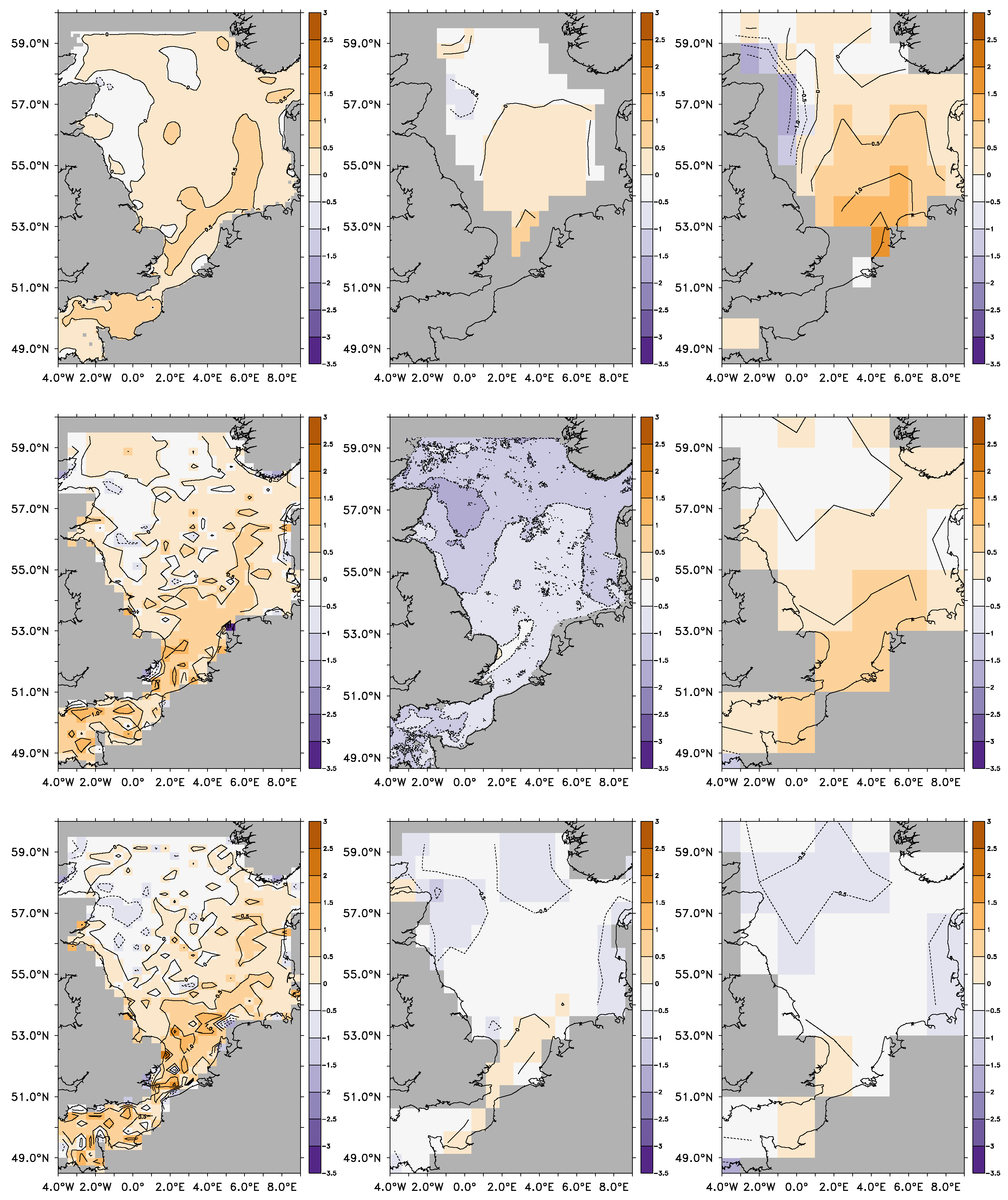
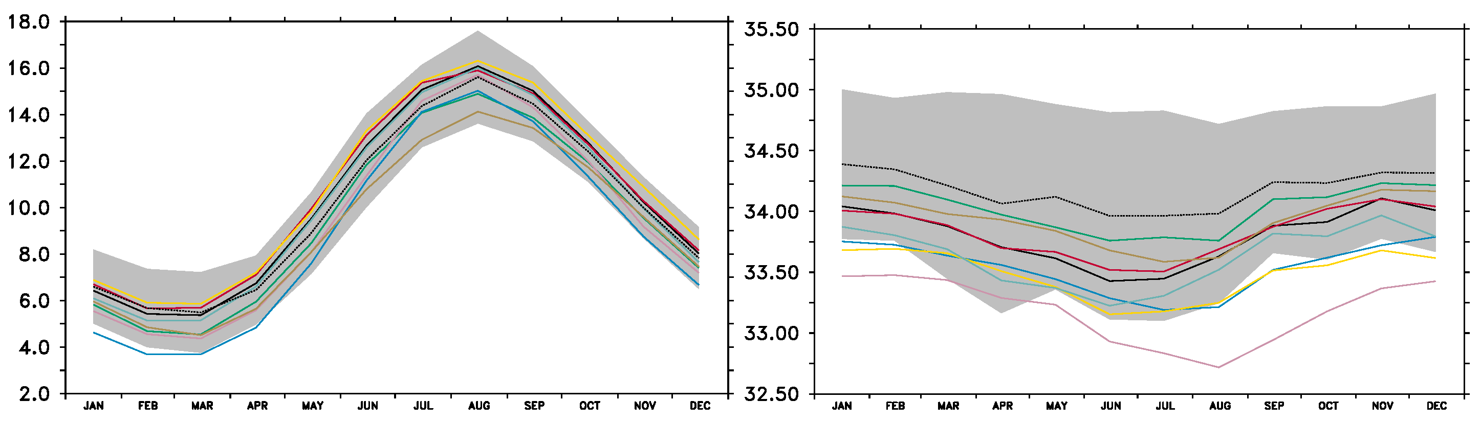
4.1. SST in the ERA40 Hindcast

The comparison of climatological annual mean SSTs in the North Sea reveals a consistent pattern of SST biases across all model solutions. Figure 1 summarizes annual mean SST biases of the ERA40 hindcast relative to different datasets. The averaging periods are not identical among the different datasets but the model results have been averaged according to the available periods in the different datasets. Figure 1 shows the SST biases relative to the KLIWAS North Sea Climatology (KNSC) compiled by Bersch et al. [46]. Figure 1 shows the bias relative to the same dataset but for the period 1980 to 2009. Along the coasts of Scotland and North East England the modeled SSTs tend to be up to −0.5 ${}^{\circ }$C colder than the SSTs derived from the observational dataset. The southern limit of the cold bias approximately coincides with the 50 m isobath and is most likely related to the inflow path of Atlantic water. In the English Channel, the Southern Bight and further to the north east where the influence of the inflow from the English Channel is strongest the model solution is 0.5 ${}^{\circ }$C to 1 ${}^{\circ }$C warmer than the SSTs from the KNSC dataset.

This general pattern is also apparent in the comparisons with the ICES climatology by Berx and Hughes [47], the Hamburg Ocean Atmosphere Parameters and Fluxes from Satellite Data (HOAPS3) [48,49], and the Atlas of Surface Marine Data 1994 (ASMD94) [50] (upper row in Figure 1). The same pattern, with different absolute values though, emerges from a comparison with the BSH SST dataset [51]. The negative bias in SSTs is smallest in the English Channel and in the Southern Bight. The strongest negative bias is found in the north western part of the North Sea. The SSTs compiled by the BSH are about 1 ${}^{\circ }$C colder than the other climatological means and the model solution. This could be related to the different averaging periods. The biases relative to the BSH SSTs are shown for the period 1990 to 2009. After the year 2002 ERA interim and ERA40 are using different sources for SSTs [52]. The biases relative to ERA interim and ERA40 SSTs during the period 1980 to 2009 (Figure 1) are negative too, while the bias relative to ERA40 in the earlier period 1970 to 1999 is slightly positive. The comparison with the KNSC dataset shows a similar dependency on the averaging period. Biases including the decade 2000 to 2009 are more positive than biases that do not include it. This could indicate that the model biases exhibit interdecadal variability. A comparison between the different datasets is beyond the scope of this study. Using several datasets however helps to establish a qualitative estimate of the spread among different datasets. For the present case of small model biases in SST (<0.5 ${}^{\circ }$C) that are within the range of the spread among different datasets it yields evidence which model biases are significant and need to be reduced in future model versions.

The warm bias in the southern parts of the North Sea is likely to be caused by an overestimation of the inflow of warm and salty Atlantic water through the English Channel (cf. Supplementary Materials). The bulk of the transport through the Channel follows the deeper isobath northward to the Outer Silver Pit where it is joined by Atlantic water flowing southward along the British Coast from the northern part of the North Sea. From here the transport route is mainly eastward along the 40 m isobath, which it follows northward through the gap between the Great and Little Fisher Banks. Those are also the regions where the warm SST bias is largest implying that water advected from the Atlantic is warmer than water that has been modified locally by processes in the North Sea.

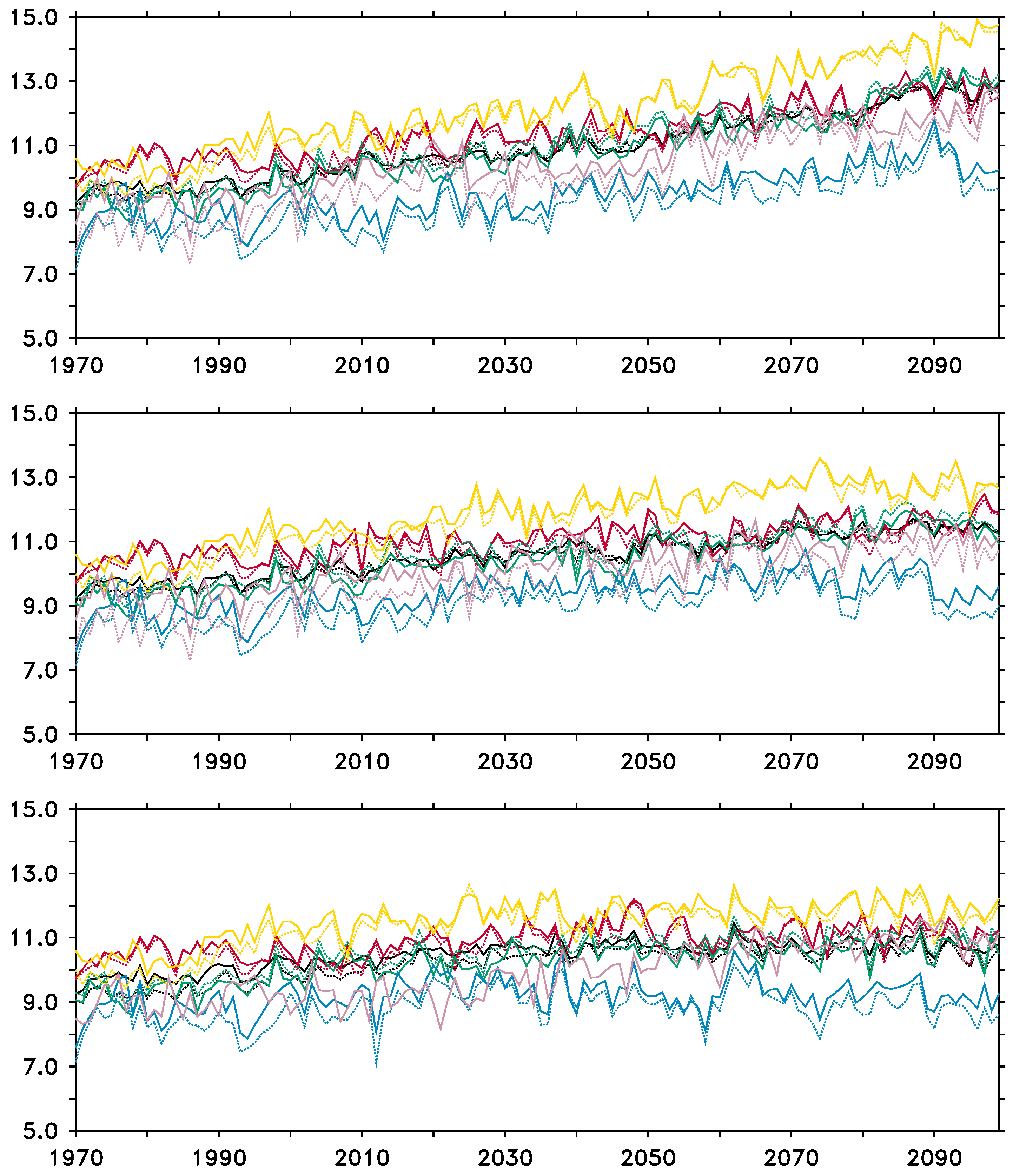
4.2. SST in the Historical Period of the Scenarios

Overall the pattern of SST biases for the historical periods (P0) of the scenario simulations (Figure 2) is very similar to the one of the ERA40 hindcast. Lower than observed SSTs along the coasts of Scotland and North East England (ICES box 3a, e.g., Lenhart and Pohlmann [53]), higher than observed SSTs in the southern and south eastern part of the North Sea where water from the English Channel dominates. The fact that all experiments show the same pattern in SST biases let us conclude that the SST biases are most likely due to model deficiencies in the ocean model. The atmospheric forcing over the North Sea is quite different in these experiments and is unlikely to cause consistent bias patterns in SST. The different atmospheric forcing is however responsible for the different absolute bias in the SST. According to Figure 2 the period P0 of the RCA4-NEMO ECHAM5 scenario is among the coldest and the same period of the RCA4-NEMO MPI-ESM-LR scenario is among the warmest compared to the same dataset. SST biases in the downscaled EC-EARTH, GFDL-ESM2M, and IPSL-CM5A-MR scenarios are predominantly negative. The historical periods in the downscaled MPI-ESM-LR and HadGEM2-ES are warmer than the KNSC dataset. This yields an ensemble mean (Figure 2) and an ensemble median (not shown) closer to the dataset than any of the individual model runs. This is a promising result and shows that ensemble modeling can be used to reduce model biases. The SST in the ocean only hindcast is slightly colder than in the coupled ERA40 hindcast but shows the same pattern in its bias to the observations. In general, the annual SST biases are smaller than ±1 ${}^{\circ }$C. Given the discrepancies on annual mean SST among different datasets, the modeled SST fields can be considered close to the actual climatology.

Judging from the climatological seasonal cycles averaged over the North Sea, in Figure 3 all model solutions for SST are within the 95% confidence limits of the observed seasonal cycle (KNSC), except for the run RCA4-NEMO GFDL-ESM2M. This run is too cold, which is also apparent in Figure 2. The biases of the two hindcasts are within 0.5 ${}^{\circ }$C of the range of the observed seasonal cycle, although the model solutions are colder during winter and warmer during summer.

The averaged climatological seasonal cycles of SSS are within the 95% confidence limits of the SSS from KNSC for some model runs. There is a clear tendency for all model runs to be too fresh and more details are discussed in the Supplementary Materials.

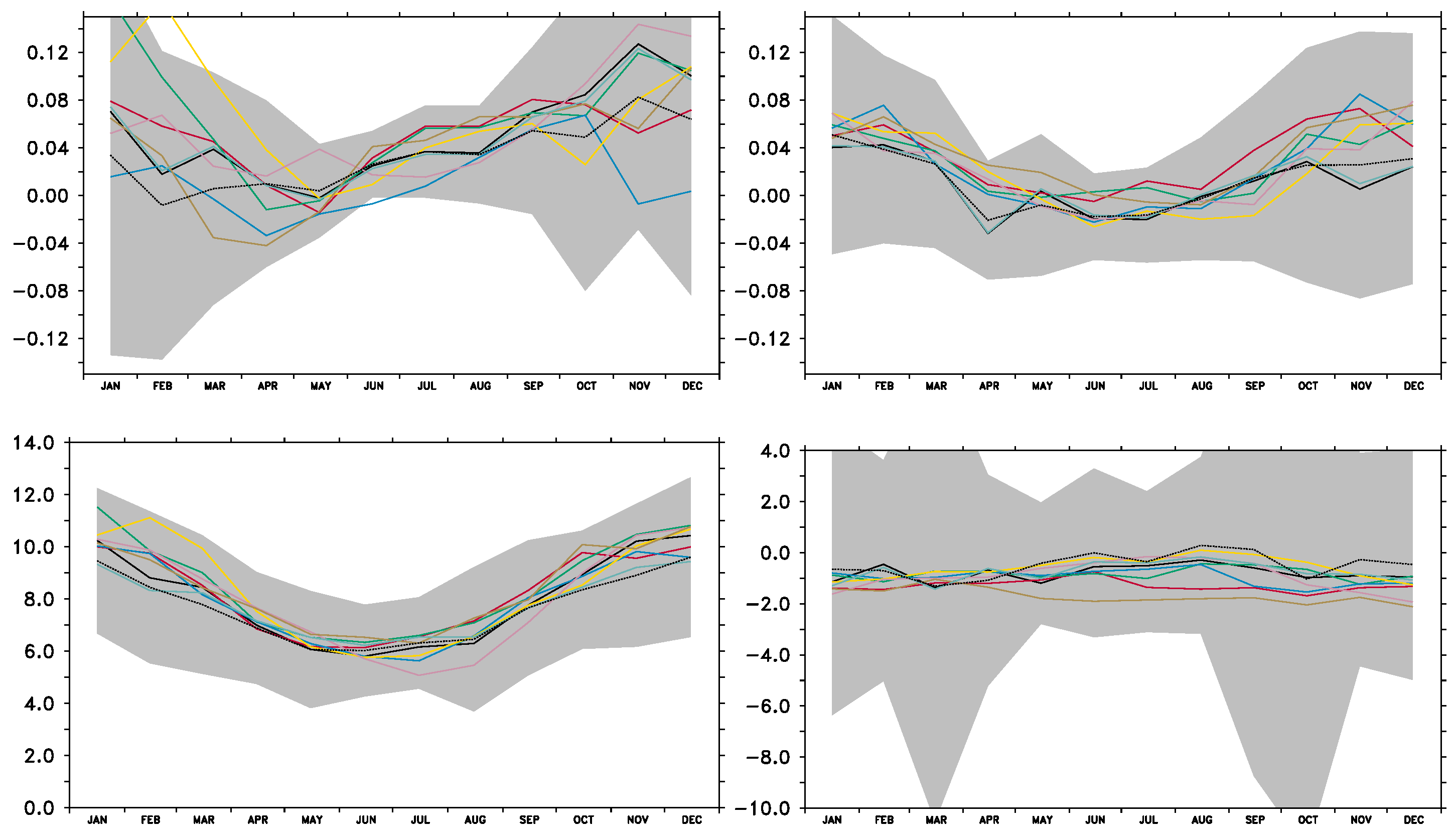
4.3. Validation of Air–Sea Fluxes

The SST in the North Sea is mainly determined locally by air–sea fluxes (e.g., [30,54,55,56]) rather than by exchange with the Atlantic Ocean or the Baltic Sea.

Table 3. Summary of climatological annual mean heat fluxes (W/m${}^2$) during period P0 averaged over the North Sea for RCA4-NEMO hindcast and scenario experiments. The values for the atmosphere only ERA40 hindcast are listed as well. The last two rows represent data from Light Vessel Elbe 1 (LVE1) and Ocean Weather Ship Famita (OWSF) published by Moll and Radach [58]. The abbreviations for the heat flux components are shortwave radiation (Q${}_{\mathrm{sw}}$), longwave radiation (Q${}_{\mathrm{lw}}$), sensible heat flux (Q${}_{\mathrm{sh}}$), latent heat flux (Q${}_{\mathrm{lh}}$), non-solar heat flux (Q${}_{\mathrm{ns}}$), and net heat flux (Q${}_{\mathrm{net}}$), respectively, with Q${}_{\mathrm{net}}$ = Q${}_{\mathrm{sw}}$ + Q${}_{\mathrm{ns}}$ = Q${}_{\mathrm{sw}}$ + Q${}_{\mathrm{lw}}$ + Q${}_{\mathrm{sh}}$ + Q${}_{\mathrm{lh}}$. Becker [57] reports an average of −5 W/m${}^2$ net heat flux for the North Sea.

	Q${}_{\mathbf{sw}}$	Q${}_{\mathbf{lw}}$	Q${}_{\mathbf{sh}}$	Q${}_{\mathbf{lh}}$	Q${}_{\mathbf{ns}}$	Q${}_{\mathbf{net}}$
ERA40	114	−54	−10	−57	−121	−7
Ensemble mean	118	−59	−11	−58	−128	−10
MPI-ESM-LR	117	−57	−9	−58	−124	−7
EC-EARTH	121	−61	−11	−59	−131	−10
GFDL-ESM2M	120	−61	−14	−57	−132	−12
HadGEM2-ES	118	−59	−10	−63	−132	−14
IPSL-CM5A-MR	116	−56	−10	−54	−120	−4
ECHAM5	109	−62	−9	−51	−122	−13
atmos only	114	−53	−10	−54	−117	−3
LVE1	113	−62	−15	−51	−128	−15
OWSF	105	−60	−12	−49	−121	−16

indicates that the RCA4-NEMO solutions yield a net heat loss for the North Sea of −4 to −14 W/m${}^2$. At the lower end of the range is the atmosphere only run which tends to have a more balanced surface heat budget. The climatological annual mean heat losses over the North Sea of different model realizations may be compared to the value of −5 W/m${}^2$ by Becker [57]. The annual mean figures for the different heat flux components are listed in Table 3. There is an agreement between model results and observations on how much each component contributes to the total heat flux. Longwave back radiation and latent heat loss both contribute approximately equally to the heat loss of the North Sea while the sensible heat loss contributes with about 10% of the total.

The shortwave radiation depicted in Figure 4 is larger than the North Sea average for the ASMD94. All simulated climatological shortwave radiation is higher during winter than ASMD94. A comparison with station data from the radiation network of the SMHI also shows a slight overestimation of shortwave radiation in the downscaled ERA40 hindcast. The bias in shortwave radiation during winter is much less pronounced, though. Longwave radiation tends to be rather constant over the year (Figure 4) and uniform in space (not shown). Most model solutions show a larger net longwave radiation from the North Sea than the climatology according to ASMD94. The RCM driven with GFDL-ESM2M and ECHAM5 are significantly biased.

The sensible and latent heat flux vary with the season. During summer when the difference between air temperature and SST is small the sensible heat loss is at its minimum. In winter the atmosphere is usually much colder than the North Sea and the sensible heat loss increases. The model solutions underestimate the sensible heat loss in winter compared to ASMD94 but are still within the 95% confidence limits. The latent heat loss in the model solutions is below the observed climatology throughout the year, although the bias is not significant at the 95% level. The −10 to −15 W/m${}^2$ stronger latent heat loss in the model solutions can be backtracked to an anomalously dry model atmosphere above the North Sea. The relative humidity during the warm half year is 5% to 10% below the observed one (not shown) according to the ASMD94. This favors extra evaporation in the model solutions. The non-solar heat fluxes show a negative bias (not significant) compared to ASMD94 and the net heat flux is slightly overestimated.

The bulk of freshwater input into the North Sea is mainly by Baltic Sea outflow and river discharge [59] An estimate has been given in Section 2. Additionally, the North Sea receives a surplus in net precipitation as shown in Figure 5. There are large uncertainties in the data due to a high interannual variability. However, the data agree with the model solutions.

For the heat exchange of the North Sea the momentum flux is of major importance since it provides mechanical energy to stir the upper part of the water column, deepen the mixed layer, and increase the thermal inertia of the North Sea. In a semi-enclosed basin like the North Sea the Ekman transport induced by the wind stress generates upwelling and downwelling circulation [60] that acts to modulate the interaction between atmosphere and ocean. Compared to the ASMD94, Figure 5 shows a general agreement on the seasonal variation of the wind stress over the North Sea. None of the model solutions are significantly different from the observational dataset. The model solutions also agree with observations on the larger uncertainty during winter. There are, however, large discrepancies between different driving GCMs. The historical period of RCA4-NEMO EC-EARTH exhibits a strong eastward stress during fall and winter. This is in agreement with other studies that have analyzed wind conditions in GCMs over the North Sea (e.g., [61,62]). Overall the uncoupled ERA40 hindcast is in best agreement with the ASMD94.

The climatological wind speed over the North Sea (Figure 5) agrees well with the observed climatology. The historical period of RCA4-NEMO EC-EARTH and HadGEM2-ES have the highest wind speeds among the model solutions. Interestingly, during fall and winter the atmosphere only ERA40 hindcast tends to underestimate the wind speed in the climatological average compared to the coupled model solutions and compared to ASMD94.

5. Results

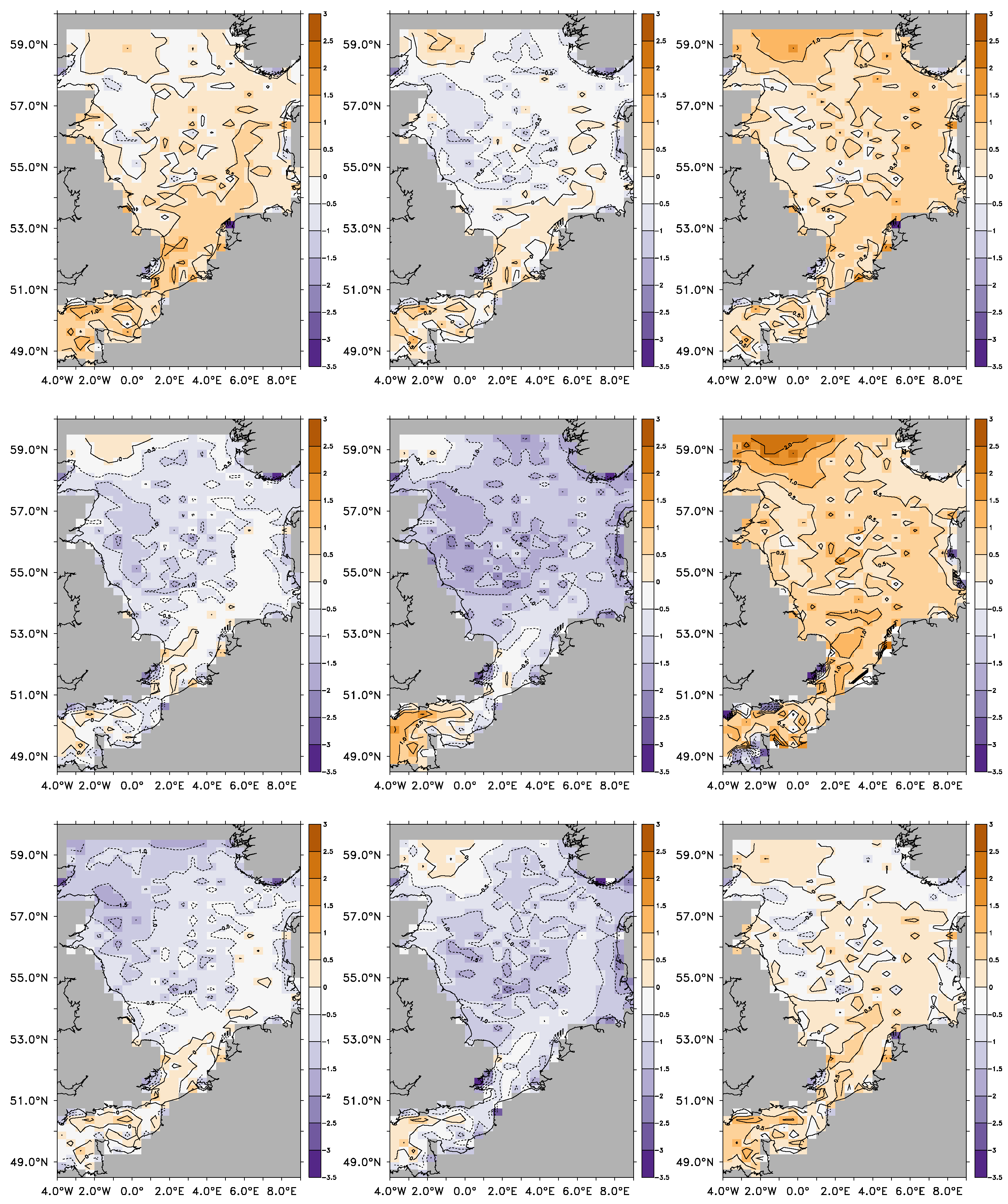
5.1. Climate Change Signal

The climate change signal derived from the individual ensemble members of the scenario runs with RCA4-NEMO is summarized in Figure 6. It shows the annual mean SST averaged over the North Sea for the 15 different scenarios listed in Table 1. The RCP8.5 scenarios show the largest SST rise in the North Sea. The ensemble median rises by 4 ${}^{\circ }$C from 9 ${}^{\circ }$C to 13 ${}^{\circ }$C between 1970 and 2100. The RCP4.5 scenarios yield an ensemble median that shows an increase of around 2 ${}^{\circ }$C and in the RCP2.6 scenarios the North Sea warms by around 1.5 ${}^{\circ }$C. The SRES A1B scenario using ECHAM5 yields an intermediate increase in SST between RCP4.5 and RCP8.5 of 2 to 3 ${}^{\circ }$C starting from 8 to 9 ${}^{\circ }$C in 1970. This is in agreement with recent studies by Gröger et al. [63] and Mathis et al. [20] who found an SST increase of 2 ${}^{\circ }$C for the North Sea in the ECHAM5 A1B scenario. In all the different RCPs the downscaled GFDL-ESM2M is the coldest and the downscaled HadGEM2-ES is the warmest.

The downscaled annual mean SST is only slightly different (<0.5 ${}^{\circ }$C) from the original annual mean SST from the CMIP5 GCMs (Figure 6). The annual mean curves follow closely the climate set by the GCMs, including interannual and decadal variability and the climate change signal. The climate change signal as a SST difference of the ensemble median between the far future and the recent past is 2.6 ${}^{\circ }$C, 1.6 ${}^{\circ }$C, and 0.8 ${}^{\circ }$C for the RCP8.5, RCP4.5, and RCP2.6 scenarios, respectively.

The temperature rise in the RCA4-NEMO ensemble is comparable to what has been assessed with an atmosphere only ensemble by Kjellström et al. [64] using the predecessor of RCA4. Regional downscaling of scenarios for the North Sea with ocean only models [20] shows a similar increase in temperature for the North Sea. As shown by e.g., Mathis et al. [18] uncoupled regionalizations tend to reproduce the SST of the GCMs. In a joint assessment of three coupled RCMs for the North Sea and Baltic Sea region RCA4-NEMO shows the least amount of warming in the ECHAM5 A1B scenario compared to the REMO-MPIOM and REMO-HAMSOM solutions [32].

In the recent past (period P0) the dispersion in the RCP8.5 ensemble is 1 ${}^{\circ }$C and increases slightly to 1.3 ${}^{\circ }$C in the far future (period P2). This is also shown in Figure 7. The ensemble members agree best in the English Channel, the Southern Bight, and the German Bight where the ensemble dispersion is below 1.3 ${}^{\circ }$C. In the central western part of the North Sea, in the Norwegian Coastal Current, and in the northern North Sea the models disagree more, up to 1.5 ${}^{\circ }$C near the open boundary. Compared to the average increase in SST of almost 4 ${}^{\circ }$C in the RCP8.5 ensemble (Figure 6) the ensemble spread is relatively small and indicates a robust ensemble solution for the SST in the North Sea. An assessment of the significance of the SST rise in the RCP8.5 ensemble for the North Sea is given in Figure 7. The figure shows the signal-to-noise ratio of the ensemble during P2. Values greater than 2 indicate a climate change signal twice as large as the ensemble dispersion. In the western North Sea where inflow from the Atlantic, upwelling and NAO sensitivity modulates the SST increase, the climate change signal is less significant than in other parts of the North Sea.

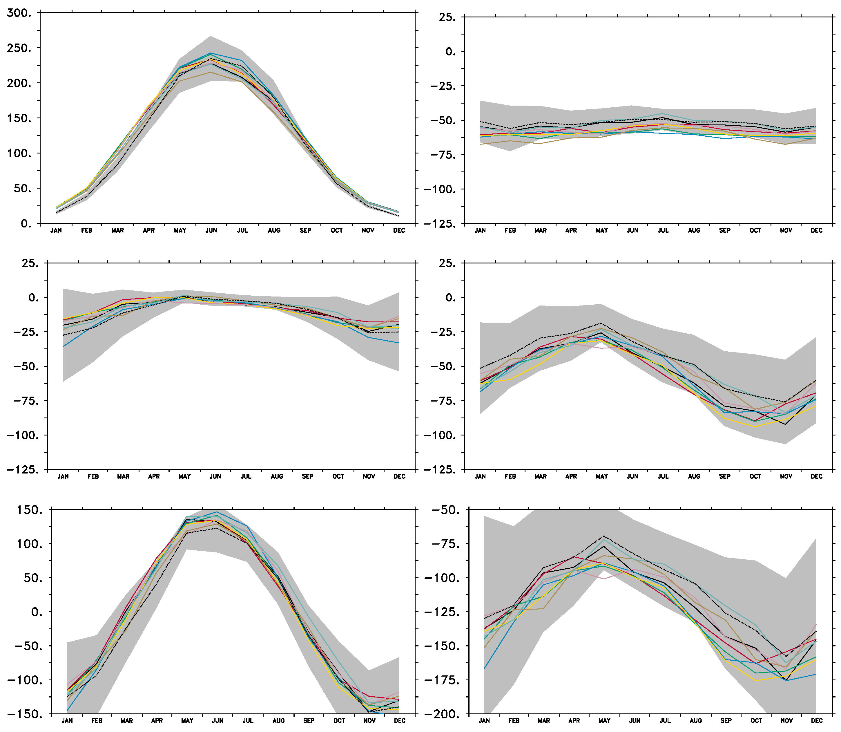
5.2. Surface Heat Budget

Table 3 has established that the ERA40 hindcast and the historical periods of the scenarios yield an overall heat budget at the surface of the North Sea that is close to estimates based on observations. In

Table 4. Summary of climatological annual mean heat fluxes (W/m${}^2$) during the three different climatological periods averaged over the North Sea for the ensemble mean of the RCA4-NEMO scenario experiments. The first three rows list the different heat flux components, respectively, and the last row lists the changes between periods P0 and P2.

	Q${}_{\mathbf{sw}}$	Q${}_{\mathbf{lw}}$	Q${}_{\mathbf{sh}}$	Q${}_{\mathbf{lh}}$	Q${}_{\mathbf{ns}}$	Q${}_{\mathbf{net}}$
RCP2.6 P2	118	−59	−10	−59	−128	−10
RCP2.6 P1	117	−59	−10	−59	−128	−11
RCP2.6 P0	118	−59	−11	−58	−128	−10
RCP2.6 P2−P0	0	0	1	−1	0	0
RCP4.5 P2	115	−55	−9	−60	−124	−9
RCP4.5 P1	117	−57	−9	−59	−125	−8
RCP4.5 P0	118	−59	−11	−58	−128	−10
RCP4.5 P2−P0	−3	4	2	−2	4	1
RCP8.5 P2	111	−50	−8	−60	−118	−7
RCP8.5 P1	116	−56	−9	−59	−124	−8
RCP8.5 P0	118	−59	−11	−58	−128	−10
RCP8.5 P2−P0	−7	9	3	−2	10	3

the changes in the surface heat budget are listed that are derived from the ensemble means of the three different RCP scenarios. In total, the North Sea does not take up more heat between 2070 and 2099 (period P2) and the last 30 years of the past century 1970 to 1999 (period P0). Only the RCP8.5 scenario shows a slight increase in heat gain over heat loss of 3 W/m${}^2$ which is not significantly different from 0.

However, the balance between the fluxes how the North Sea and the overlying atmosphere exchange heat shifts from period P0 to period P2. In the following, we discuss and show annual mean changes between periods P0 and P2, since those changes are more robust than changes for just one season. Most of the spatial variations seen in the annual changes are caused by changes in summer however. The five members of the RCP8.5 ensemble show the most pronounced changes and are used to discuss the changing surface heat budget of the North Sea. Qualitatively, the RCP4.5 ensemble shows the same changes as the RCP8.5 ensemble, although with a smaller amplitude. The changes in the RCP2.6 ensemble are small and do not exhibit the patterns seen in the RCP4.5 and 8.5 ensemble.

According to Table 4 the increased greenhouse effect at the end of the century provides up to 9 W/m${}^2$ more net longwave radiation averaged over the North Sea for the ensemble mean of the RCP8.5 scenarios. At the same time the shortwave radiation reduces by 7 W/m${}^2$ due to an increase in total cloud cover (Figure 8). The decrease in sensible heat loss is of the order of 3 W/m${}^2$ for the ensemble mean. This could indicate that the temperature difference between atmosphere and ocean gets smaller, specially during winter when the sensible heat loss of the ocean is highest. Between periods P0 and P2 the latent heat loss increases by 2 W/m${}^2$. There is a number of variables that affect latent heat loss namely wind speed, atmospheric temperature, relative humidity, and SST.

Even though the net heat loss averaged over the North Sea does not change much between periods P0 and P2, there is a distinct area in the central western North Sea where the net heat loss to the atmosphere increases consistently between periods P0 and P1 and between periods P1 and P2 (Figure 8). To make up for the more or less constant heat balance the net heat loss in the German Bight, the outflow region of the Baltic Sea, and the northern North Sea decreases. The amplitude of this spatial signal (5 W/m${}^2$) is comparable to a radiative forcing due to a CO${}_2$ doubling. From Figure 8 it is also evident that the non-solar heat fluxes are responsible for the change in the pattern of the annual mean heat exchange. The changes in shortwave radiation (Figure 8) in the central western North Sea between P0 and P2 are of the order of −7 W/m${}^2$ and are relatively uniformly distributed. The signal does not vary by more than 1 W/m${}^2$ across the North Sea. The reduction in net shortwave radiation seems to be closely related to an increase in total cloud cover (Figure 8) over the area. Changes in total cloud cover are of the order of 2% which is matched by the change in shortwave radiation [65].

The annual changes between P0 and P2 for the different components of the non-solar heat flux are shown in Figure 9. While the sensible heat flux and the longwave radiation show a reduced heat loss during P2, the reduction is smaller by approximately 2 W/m${}^2$ in the central western North Sea. The heat loss due to latent heat flux increases and it is larger by 4 W/m${}^2$ in the central western North Sea. The pattern of increased latent heat loss is different from the other two components and is more closely related to changes in the atmosphere–ocean temperature difference (Figure 10).

The development of atmosphere–ocean temperature difference (<0.1 ${}^{\circ }$C) indicates that the central western North Sea is warming up as quickly as the atmosphere above it. Considering the linear dependency of sensible heat flux on temperature difference explains why changes in sensible heat flux in the central western North Sea are small.

The changes in longwave radiation between P0 and P2 are of the order 9 W/m${}^2$. The spatial variations of longwave radiation changes over the North Sea are small (<1 W/m${}^2$). This reflects the low sensitivity against changes in either SST or air temperature but a high correlation to cloud cover.

The most pronounced changes are found in the latent heat flux. In the central western North Sea the latent heat loss increases by up to 5 W/m${}^2$, while changes in the eastern part of the North Sea are less than ±2 W/m${}^2$. The latent heat flux strongly depends on the relative humidity (Figure 9), which decreases over the whole North Sea region. Even though the specific humidity increases in all the scenarios throughout the model domain (not shown) the increase in 2 m temperature is faster than the increase in dew-point temperature which leads to a relatively drier atmosphere near the surface during period P2 compared to period P0.

6. Discussion

The SST changes between periods P0 and P2 (Figure 10) show a distinct pattern of larger changes (>2.1 ${}^{\circ }$C) in the central western North Sea between the Wash in the south and the Firth of Forth in the north where the North Sea is relatively deep. Northeast of the Dogger Bank there is also an area with large SST changes. In principle the area where SST increases fastest corresponds to the ICES North Sea box 7a [53]. Figure 10 reveals that not only the SST but also the vertical mean temperature of the North Sea increases most rapidly in this area. The pattern in SST changes is found during the warmer half of the year and is representative for summer.

There are several possible explanations why the North Sea warms up with a specific spatial pattern. At first, the cause for SST changes on small spatial scales would be expected in the ocean. It cannot be ruled, out however that the atmosphere feeds back onto the ocean on a local scale when changes in land–sea circulations become more pronounced. With a resolution of ∼25 km, RCA4 does not resolve land–sea breeze circulation but that does not eliminate the potential for feedback between land surfaces and open water. Figure 10 clearly shows that the land–sea surface temperature contrast is intensifying.

Possible hypotheses for the SST changes under changing large-scale conditions observed in the RCA4-NEMO scenarios include (1) covariation with the NAO index, (2) increase in lateral heat transports, (3) changes in the structure of the stratification, (4) strengthening of the Ekman transport, and (5) changes in atmosphere–ocean interaction.

6.1. Covariation with the NAO Index

The area where the SST increases fastest corresponds to the area of high correlation with the North Atlantic Oscillation (NAO) index identified by Becker and Pauly [55]. The modeled winter NAO index calculated as a station based sea level pressure (SLP) difference between Lisbon and Reykjavik corresponds well with the data compiled by Hurrell [66]. The correlation between the RCA4-NEMO ERA40 derived NAO index and the one inferred from observations is 0.94 with a rms error of 0.38. There is a tendency for more frequent positive and stronger NAO+ phases in the RCA4-NEMO scenarios, especially in the ones driven by RCP8.5. This is in agreement with other studies [67,68,69] that have shown that the westerlies over the Atlantic Ocean increase in most of the RCP8.5 scenarios conducted under CMIP5. Changes in NAO index inferred from the RCA4-NEMO scenarios are small, inconsistent and probably not significant and do not offer a plausible explanation for extra warming in the central western North Sea.

6.2. Increase in Lateral Heat Transports

The advective heat transport was determined from daily values of volume transport and temperature across the North Sea Ocean Observing System (NOOS) sections N4 plus N5, N9, and N13 (cf. Supplementary Materials). Therefore the contribution of tides to the advective heat transport is not included. The advective heat transport is calculated relative to a temperature of 6 ${}^{\circ }$C. The Baltic Sea is the smallest contributor of heat to the North Sea for all members of the RCP8.5 ensemble. Approximately an order of magnitude less than the heat exchange with the Atlantic through the northern North Sea and through the English Channel. The Baltic Sea changes from a heat source of the North Sea to a heat sink during the 21st century. The English Channel is the largest heat source to the North Sea and tends to decrease during the century. Its contribution is however balanced by the increasing inflow of heat from the North East Atlantic through the open boundary in the northern North Sea. Overall the lateral heat transport into the North Sea does not change significantly until 2100 compared to the interannual variability. The difference in total advective heat transport between periods P0 and P2 amounts to −0.4 TW for the ensemble median. This would be equivalent to a change in surface heat flux of 0.7 W/m${}^2$. This is well within the noise level of what has been discussed in the previous section. The changing contributions from the English Channel and from the North East Atlantic could however contribute to an asymmetric temperature signal in the North Sea. Further, the model underestimates volume transports and consequently also lateral heat transports.

6.3. Changes in the Structure of the Stratification

During period P2 the stratification in the North Sea is stronger than in period P0 (Figure 11). As a measure of stratification we use potential energy anomaly (PEA) as defined by Holt et al. [70]. The amount of energy necessary to completely mix the water column indicates the strength of the stratification. During period P0 the distribution of PEA shows that the North Sea south of the line Flamborough Head to Cuxhaven is well mixed with values of PEA less than 10 J/m${}^3$ [70]. The shallow area off Jutland and the Dogger Bank are also well mixed during the whole year, as indicated by low values in ensemble mean PEA for period P0. The solution for PEA in the RCA4-NEMO ERA40 hindcast looks very similar to the ensemble mean in Figure 11 and is not shown here. It is interesting to note that the river plumes of Seine, Rhine/Meuse/Scheldt/Ijssel, and Ems/Jade/Weser/Elbe leave an imprint in the stratification. The change in PEA between periods P0 and P2 indicates that all over the North Sea the stratification strengthens except for those areas that are well mixed. The region off the coast of Scotland where upwelling occurs also frequently tends not to become more stratified. A stronger stratification along with increasing temperatures implies that SSTs are increasing faster than the depth averaged temperature. The region where PEA increases by more than 20 J/m${}^3$ matches the one where the specific heat content of the North Sea increases by more than 0.5 GJ/m${}^2$ (not shown). Stronger stratification and higher heat content have opposite effects on the oceans capacity to dampen atmospheric variability and to provide a lag in seasonal heating and cooling of the atmosphere over the North Sea. For the long-term evolution of the SST a strengthening stratification leads to a tighter coupling between atmosphere and ocean with reduced air–sea temperature differences. That matches the tendency discussed in Section 5. The pattern how PEA changes between periods P0 and P2 does not match the changing heat flux pattern, though.

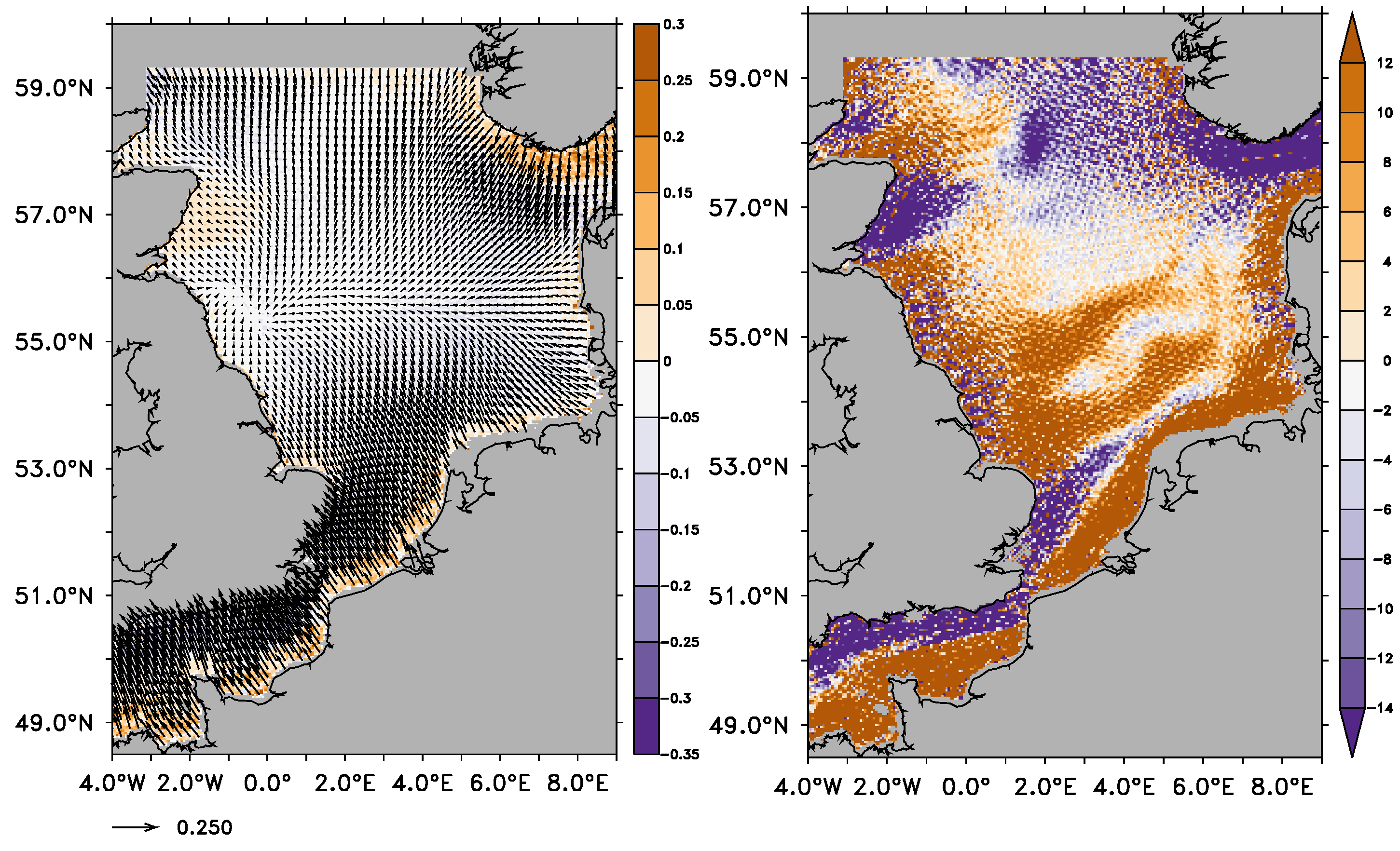
6.4. Strengthening of the Ekman Transport

The central western North Sea experiences a more convergent Ekman transport in period P2 compared to period P0 as indicated in Figure 12. First of all, this convergent transport acts to accumulate heat and strengthen the thermocline, and thus increase the SST in the region. The convergent Ekman transport is accompanied by an increase in downward Ekman pumping velocity. A crude estimate of the effect of the convergent Ekman transport on the heat budget is given in Figure 12. It shows an increase in heat flux calculated as the difference in climatological means between periods P0 and P2 of the heat flux divergence. The monthly heat flux divergence is calculated as the product of the monthly mean Ekman transport and the monthly mean SST. The positive extremes of the Ekman-induced heat flux changes are situated along the coast of the continent where there is reduced downwelling (Figure 12). Along the coast of southern Norway and the coasts of Great Britain that are oriented southwest to northeast the upwelling increases and contributes to a reduced heat flux. The average additional heat flux during P2 compared to P0 in the ICES boxes 7a plus 7b is 4.7 W/m${}^2$. For the ICES boxes 7a alone it is 1.8 W/m${}^2$. Clearly, the changing Ekman transports are a factor in the surface heat budget of the North Sea although not all of this heat flux is available to heat the surface layer.

6.5. Changes in Atmosphere–Ocean Interaction

The mean radiative forcing of the North Sea is of the order of 50 W/m${}^2$ for the recent past (Figure 4; 59 W/m${}^2$ according to Table 3). Prandle and Lane [54] showed that the equilibrium air–sea temperature difference for the North Sea can be approximated by the radiative forcing divided by the efficiency how heat is exchanged between ocean and atmosphere. With an efficiency of 50 W/m${}^2$ ${}^{\circ }$C [54], this yields an air–sea temperature difference of the order of −1 ${}^{\circ }$C for the recent past, which fits well with the RCA4-NEMO scenarios, both for the spatial mean over the North Sea and the annual mean over a 30-year climatological period.

Since the spatial variability in changes of the radiative heating between periods P0 and P2 is small (Figure 13), the more likely candidate for the spatial pattern in the air–sea temperature difference in Figure 10 is the changing efficiency of vertical heat exchange (Figure 13). The reciprocal efficiency reduces by approximately 1/20 m${}^2$ ${}^{\circ }$C/W. This would decrease the air–sea temperature difference by approximately 0.3 ${}^{\circ }$C, which matches what is shown in Figure 10.

From Figure 13 it is apparent that the changes in wind speed are insignificant and not responsible for the increased efficiency of vertical heat exchange.

An equivalent equilibrium SST can be expressed by the sum of the dew point temperature and the climatological shortwave radiation divided by the heat exchange efficiency [71]. From Figure 8 it is apparent that the shortwave radiation changes uniformly across the North Sea by approximately −6 W/m${}^2$. Ignoring spatial variations in the efficiency for the moment, this change implies a reduction in SST of the order of −0.1 ${}^{\circ }$C. What is observed in Figure 10 are changes in the central western North Sea of 0.4 ${}^{\circ }$C compared to the rest of the North Sea. An increase in dew point temperatures would increase the SST which is shown in Figure 13. The southern North Sea region shows smaller increase in dew point temperatures during period P2 than regions further north. Drier air is advected from the British Isles over the North Sea (Figure 8) and moderates the increase in dew point temperatures. In thermal equilibrium, this would increase the SSTs by about 0.2 ${}^{\circ }$C. At the same time a long-term mean SST must be balanced by the near surface air temperature plus the radiative heat transfer divided by the heat exchange efficiency. The local increase in SST is also controlled by the longwave back radiation which increases strongly with increasing SST.

7. Summary and Conclusions

For this paper an ensemble of five GCMs with three RCPs has been downscaled for the North Sea and Baltic Sea. The results for the North Sea in the ERA40 hindcast with RCA4-NEMO compares well with climatological means and seasonal cycles derived from observational datasets. This also applies to the historical periods in the scenario simulations with RCA4-NEMO. The SST in the North Sea is within the range of the observed ones. The SSS is too low and is partly the result of high precipitations rates over the Baltic Sea and weak vertical mixing in the Norwegian Coastal Current due to an underestimation of wind speed. Volume transports across the northern boundary are weak and the model tends to produce more transport through the Strait of Dover than observed. This also affects the distribution and amount of freshwater in the North Sea. Low SSS around and downstream the large rivers mouths are not backed by gridded observational datasets and might point to model deficiencies in horizontal and vertical mixing. The momentum, heat, and freshwater exchange of the North Sea with the atmosphere are in agreement with observations both for RCA4-NEMO driven with ERA40 and with different GCMs.

The projected SST increase for the North Sea as a whole is within 1 to 5 ${}^{\circ }$C depending on the RCP. In the far future it is significantly more than the ensemble spread for both the RCP4.5 and 8.5. An increased greenhouse effect in the region is accompanied by increased air temperature and cloud cover and reduced shortwave radiation and relative humidity. The North Sea responds not uniformly to global warming according to the ensemble of RCP8.5 and RCP4.5 scenarios downscaled with RCA4-NEMO. Air–sea interaction in the central western North Sea works to reduce the air–sea temperature difference. Dry air is advected from the British Isles over the North Sea, which makes the latent heat transfer more effective.

The main findings of this paper can be summarized as follows

• We presented the first ensemble with a coupled RCM that covers the full range of RCP scenarios for the North Sea.
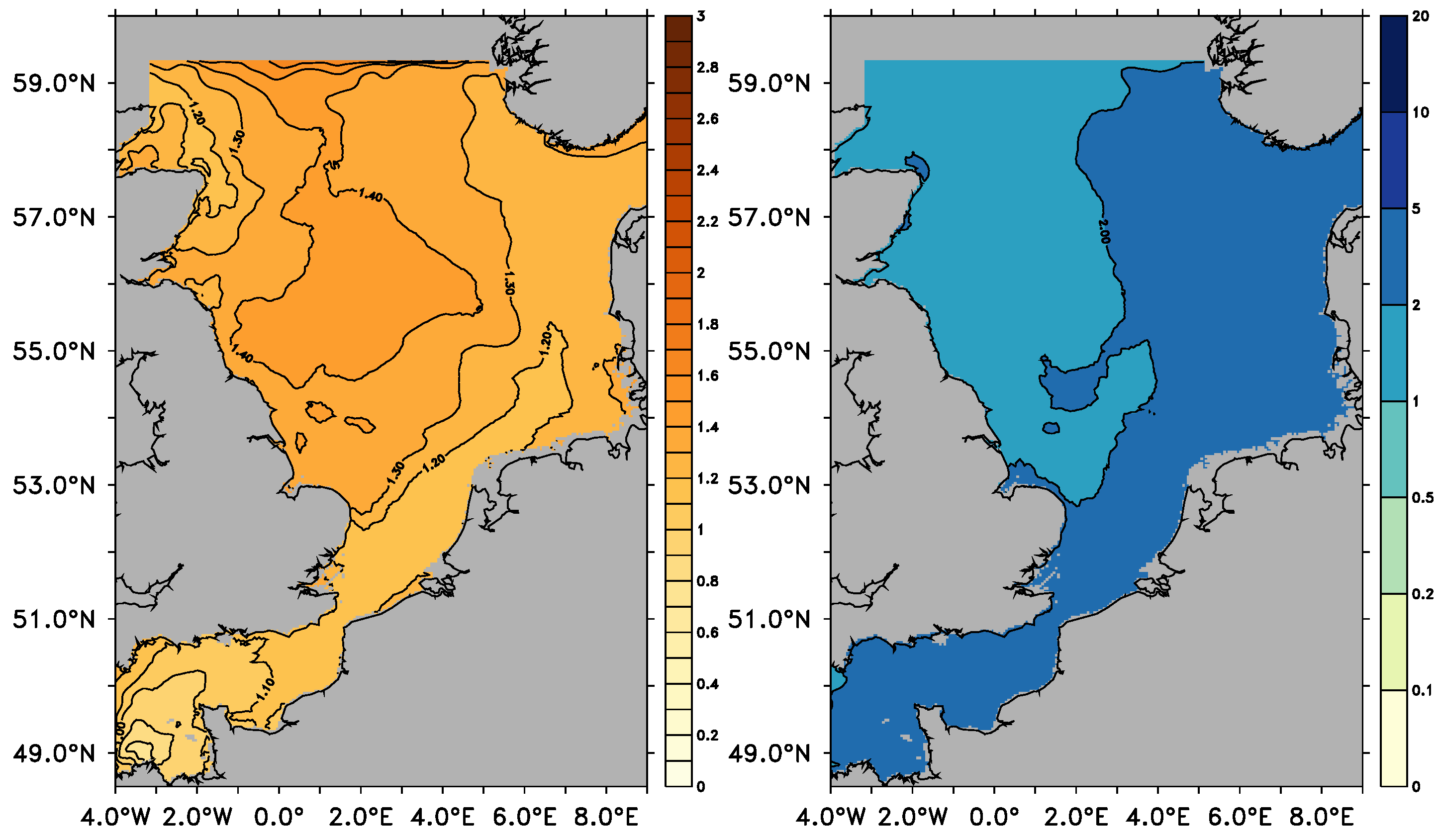
• The RCA4-NEMO North Sea SSTs are within observational estimates. Datasets agree within 1 ${}^{\circ }$C and the bias is of the same order of magnitude.
• The ensemble mean SST has a smaller bias than any individual model run. This points to the need of ensemble modeling in the future.
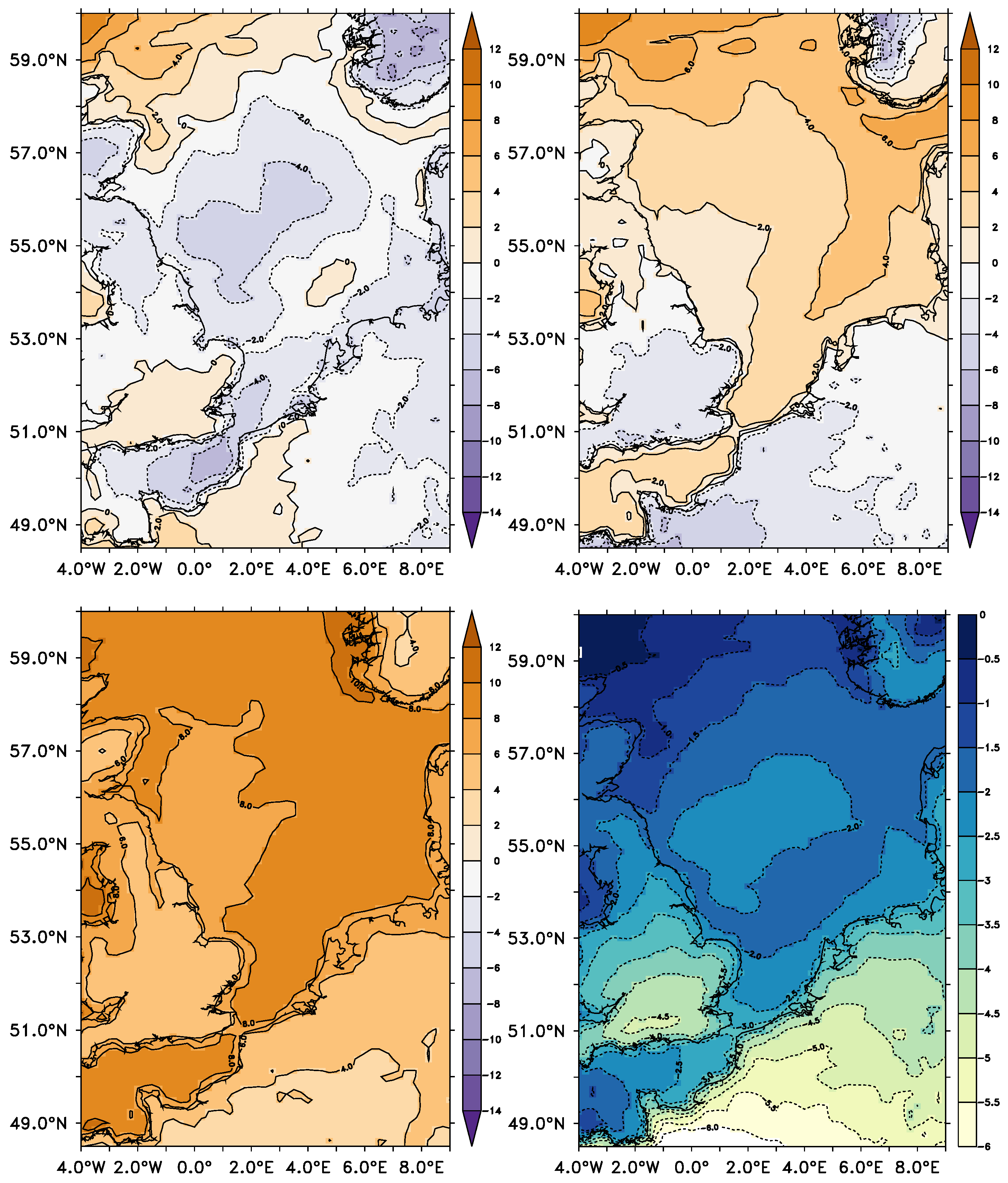
• The North Sea warms up by 1 to 5 ${}^{\circ }$C in agreement with other studies.
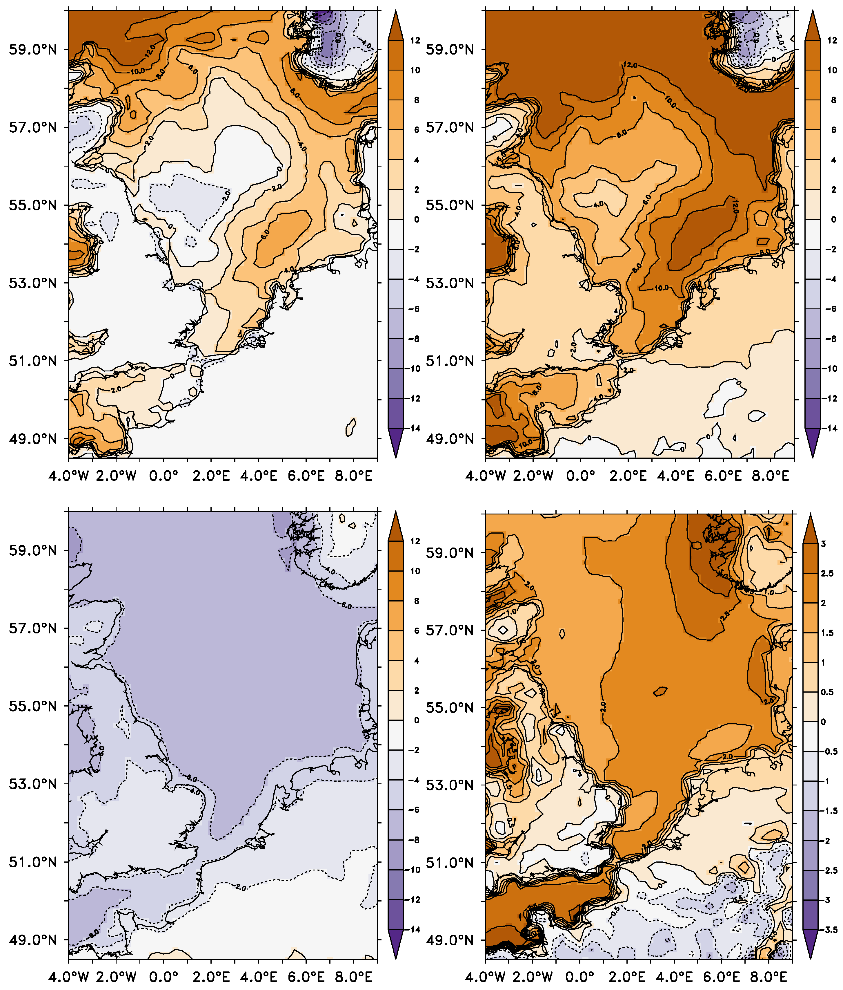
• Global warming in the North Sea leads to a shift in the balance of the surface heat fluxes. The changes in the heat fluxes show the same pattern as the changes in atmosphere–ocean temperature difference.
• A plausible explanation is an increase in the efficiency how latent heat is exchanged. That can be explained with a relatively drier atmosphere in the future which is advected from the British Isles over the North Sea.
• Our study provides an example of how changing land–sea contrast affects regional circulation patterns and feedbacks that point to the importance of regional coupled atmosphere–ocean modeling.

References

1. Wan, H.; Giorgetta, M.A.; Zängl, G.; Restelli, M.; Majewski, D.; Bonaventura, L.; Fröhlich, K.; Reinert, D.; Rípodas, P.; Kornblueh, L.; et al. The ICON-1.2 hydrostatic atmospheric dynamical core on triangular grids—Part 1: Formulation and performance of the baseline version. Geosci. Model Dev. 2013, 6, 735–763. [Google Scholar] [CrossRef]
2. Feser, F.; Rockel, B.; von Storch, H.; Winterfeldt, J.; Zahn, M. Regional Climate Models Add Value to Global Model Data: A Review and Selected Examples. Bull. Am. Meteorol. Soc. 2011, 92, 1181–1192. [Google Scholar] [CrossRef] [Green Version]
3. Meier, H.E.M.; Höglund, A.; Döscher, R.; Andersson, H.; Löptien, U.; Kjellström, E. Quality assessment of atmospheric surface fields over the Baltic Sea from an ensemble of regional climate model simulations with respect to ocean dynamics. Oceanologia 2011, 53, 193–227. [Google Scholar] [CrossRef]
4. Rummukainen, M. State-of-the-art with regional climate models. WIREs Clim. Chang. 2010, 1, 82–96. [Google Scholar] [CrossRef]
5. Gustafsson, N.; Nyberg, L.; Omstedt, A. Coupling of a High-Resolution Atmospheric Model and an Ocean Model for the Baltic Sea. Mon. Weather Rev. 1998, 126, 2822–2846. [Google Scholar] [CrossRef]
6. Hagedorn, R.; Lehmann, A.; Jacob, D. A coupled high resolution atmosphere–ocean model for the BALTEX region. Meteorol. Z. 2000, 9, 7–20. [Google Scholar] [CrossRef]
7. Döscher, R.; Willén, U.; Jones, C.; Rutgersson, A.; Meier, H.E.M.; Hansson, U.; Graham, L.P. The development of regional coupled ocean–atmosphere model RCAO. Boreal Environ. Res. 2002, 7, 183–192. [Google Scholar]
8. Schrum, C.; Hübner, U.; Jacob, D.; Podzun, R. A coupled atmosphere/ice/ocean model for the North Sea and Baltic Sea. Clim. Dyn. 2003, 21, 131–151. [Google Scholar] [CrossRef]
9. Meier, H.E.M.; Döscher, R. Simulated water and heat cycles of the Baltic Sea using a 3D coupled atmosphere–ice–ocean model. Boreal Environ. Res. 2002, 7, 327–334. [Google Scholar]
10. Lehmann, A.; Lorenz, P.; Jacob, D. Modelling the exceptional Baltic Sea inflow events in 2002–2003. Geophys. Res. Lett. 2004, 31. [Google Scholar] [CrossRef]
11. Tian, T.; Boberg, F.; Christensen, O.B.; Christensen, J.H.; She, J.; Vihma, T. Simulations of the last two decades Baltic Sea climate using a high-resolution regional climate model: A comparison using prescribed and modelled SSTs. Tellus A 2013, 65, 19951. [Google Scholar] [CrossRef]
12. Van Pham, T.; Brauch, J.; Dieterich, C.; Frueh, B.; Ahrens, B. New coupled atmosphere–ocean–ice system COSMO-CLM/NEMO: Assessing air temperature sensitivity over the North and Baltic Seas. Oceanologia 2014, 56, 167–189. [Google Scholar] [CrossRef]
13. Gröger, M.; Dieterich, C.; Meier, H.E.M.; Schimanke, S. Thermal air–sea coupling in hindcast simulations for the North Sea and Baltic Sea on the NW European shelf. Tellus A 2015, 67, 26911. [Google Scholar] [CrossRef] [Green Version]
14. Ho-Hagemann, H.T.M.; Gröger, M.; Rockel, B.; Zahn, M.; Geyer, B.; Meier, H.E.M. Effects of air–sea coupling over the North Sea and the Baltic Sea on simulated summer precipitation over Central Europe. Clim. Dyn. 2017. [Google Scholar] [CrossRef]
15. Jeworrek, J.; Wu, L.; Dieterich, C.; Rutgersson, A. Characteristics of convective snow bands along the Swedish east coast. Earth Syst. Dyn. 2017, 8, 163–175. [Google Scholar] [CrossRef] [Green Version]
16. Van Pham, T.; Brauch, J.; Früh, B.; Ahrens, B. Simulation of snowbands in the Baltic Sea area with the coupled atmosphere–ocean–ice model COSMO-CLM/NEMO. Meteorol. Z. 2017, 26, 71–82. [Google Scholar] [CrossRef]
17. Sein, D.V.; Mikolajewicz, U.; Gröger, M.; Fast, I.; Cabos, W.; Pinto, J.G.; Hagemann, S.; Semmler, T.; Jacob, D. Regionally coupled atmosphere–ocean–sea ice–marine biogeochemistry model ROM. Part I: Description and validation. J. Adv. Model. Earth Syst. 2015, 7, 268–304. [Google Scholar] [CrossRef]
18. Mathis, M.; Elizalde, A.; Mikolajewicz, U. Which complexity of regional climate system models is essential for downscaling anthropogenic climate change in the Northwest European Shelf? Clim. Dyn. 2018, 50, 2637–2659. [Google Scholar] [CrossRef]
19. Holt, J.; Butenschön, M.; Wakelin, S.L.; Artioli, Y.; Allen, J.I. Oceanic controls on the primary production of the northwest European continental shelf: Model experiments under recent past conditions and a potential future scenario. Biogeosciences 2012, 9, 97–117. [Google Scholar] [CrossRef]
20. Mathis, M.; Mayer, B.; Pohlmann, T. An uncoupled dynamical downscaling for the North Sea: Method and evaluation. Ocean Model. 2013, 72, 153–166. [Google Scholar] [CrossRef]
21. Holt, J.; Schrum, C.; Cannaby, H.; Daewel, U.; Allen, I.; Artioli, Y.; Bopp, L.; Butenschon, M.; Fach, B.A.; Harle, J.; et al. Potential impacts of climate change on the primary production of regional seas: A comparative analysis of five European seas. Prog. Oceanogr. 2016, 140, 91–115. [Google Scholar] [CrossRef] [Green Version]
22. Meier, H.E.M.; Müller-Karulis, B.; Andersson, H.C.; Dieterich, C.; Eilola, K.; Gustafsson, B.G.; Höglund, A.; Hordoir, R.; Kuznetsov, I.; Neumann, T.; et al. Impact of Climate Change on Ecological Quality Indicators and Biogeochemical Fluxes in the Baltic Sea: A Multi-Model Ensemble Study. Ambio 2012, 41, 558–573. [Google Scholar] [CrossRef] [PubMed] [Green Version]
23. Eilola, K.; Almroth-Rosell, E.; Dieterich, C.; Fransner, F.; Höglund, A.; Meier, H.E.M. Modeling Nutrient Transports and Exchanges of Nutrients Between Shallow Regions and the Open Baltic Sea in Present and Future Climate. Ambio 2012, 41, 586–599. [Google Scholar] [CrossRef] [Green Version]
24. Meier, H.E.M.; Hordoir, R.; Andersson, H.C.; Dieterich, C.; Eilola, K.; Gustafsson, B.G.; Höglund, A.; Schimanke, S. Modeling the combined impact of changing climate and changing nutrient loads on the Baltic Sea environment in an ensemble of transient simulations for 1961–2099. Clim. Dyn. 2012, 39, 2421–2441. [Google Scholar] [CrossRef] [Green Version]
25. Neumann, T.; Eilola, K.; Gustafsson, B.; Müller-Karulis, B.; Kuznetsov, I.; Meier, H.E.M.; Savchuk, O.P. Extremes of Temperature, Oxygen and Blooms in the Baltic Sea in a Changing Climate. Ambio 2012, 41, 574–585. [Google Scholar] [CrossRef] [Green Version]
26. Somot, S.; Sevault, F.; Déqué, M.; Crépon, M. 21st century climate change scenario for the Mediterranean using a coupled atmosphere–ocean regional climate model. Glob. Planet Chang. 2008, 63, 112–126. [Google Scholar] [CrossRef] [Green Version]
27. Dubois, C.; Somot, S.; Calmanti, S.; Carillo, A.; Déqué, M.; Dell’Aquilla, A.; Elizalde, A.; Gualdi, S.; Jacob, D.; L’Hévéder, B.; et al. Future projections of the surface heat and water budgets of the Mediterranean Sea in an ensemble of coupled atmosphere–ocean regional climate models. Clim. Dyn. 2012, 39, 1859–1884. [Google Scholar] [CrossRef]
28. Su, J.; Sein, D.V.; Mathis, M.; Mayer, B.; O’Driscoll, K.; Chen, X.; Mikolajewicz, U.; Pohlmann, T. Assessment of a zoomed global model for the North Sea by comparison with a conventional nested regional model. Tellus A 2014, 66, 23927. [Google Scholar] [CrossRef]
29. Dieterich, C.; Schimanke, S.; Wang, S.; Väli, G.; Liu, Y.; Hordoir, R.; Axell, L.; Höglund, A.; Meier, H.E.M. Evaluation of the SMHI Coupled Atmosphere–Ice–Ocean Model RCA4-NEMO; Report Oceanography 47; SMHI: Norrköping, Sweden, 2013. [Google Scholar]
30. Wang, S.; Dieterich, C.; Döscher, R.; Höglund, A.; Hordoir, R.; Meier, H.E.M.; Samuelsson, P.; Schimanke, S. Development and evaluation of a new regional coupled atmosphere–ocean model in the North Sea and Baltic Sea. Tellus A 2015, 67, 24284. [Google Scholar] [CrossRef]
31. Nakicenovic, N.; Alcamo, J.; Davis, G.; de Vries, B.; Fenhann, J.; Gaffin, S.; Gregory, K.; Grübler, A.; Jung, T.Y.; Kram, T.; et al. Special Report on Emissions Scenarios: A Special Report of Working Group III of the Intergovernmental Panel on Climate Change; Technical Report; IPCC: Cambridge, UK, 2000. [Google Scholar]
32. Bülow, K.; Dieterich, C.; Elizalde, A.; Gröger, M.; Heinrich, H.; Hüttl-Kabus, S.; Klein, B.; Mayer, B.; Meier, H.E.M.; Mikolajewicz, U.; et al. Comparison of Three Regional Coupled Ocean Atmosphere Models for The North Sea Under Today’s and Future Climate Conditions; KLIWAS Schriftenreihe 27/2014; KLIWAS: Koblenz, Germany, 2014. [Google Scholar] [CrossRef]
33. Yamazaki, D.; Kanae, S.; Kim, H.; Oki, T. A physically based description of floodplain inundation dynamics in a global river routing model. Water Resour. Res. 2011, 47. [Google Scholar] [CrossRef] [Green Version]
34. Samuelsson, P.; Jones, C.G.; Willén, U.; Ullerstig, A.; Gollvik, S.; Hansson, U.; Jansson, C.; Kjellström, E.; Nikulin, G.; Wyser, K. The Rossby Centre Regional Climate model RCA3: model description and performance. Tellus A 2011, 63, 4–23. [Google Scholar] [CrossRef] [Green Version]
35. Hordoir, R.; Dieterich, C.; Basu, C.; Dietze, H.; Meier, H.E.M. Freshwater outflow of the Baltic Sea and transport in the Norwegian current: A statistical correlation analysis based on a numerical experiment. Cont. Shelf Res. 2013, 64, 1–9. [Google Scholar] [CrossRef]
36. Hordoir, R.; Axell, L.; Löptien, U.; Dietze, H.; Kuznetsov, I. Influence of sea level rise on the dynamics of salt inflows in the Baltic Sea. J. Geophys. Res.-Oceans 2015, 120, 6653–6668. [Google Scholar] [CrossRef] [Green Version]
37. Madec, G. NEMO Ocean Engine, 3.3 ed.; IPSL: Paris, France, 2011. [Google Scholar]
38. Vancoppenolle, M.; Fichefet, T.; Goosse, H.; Bouillon, S.; Madec, G.; Maqueda, M.A.M. Simulating the mass balance and salinity of Arctic and Antarctic sea ice. 1. Model description and validation. Ocean Model. 2009, 27, 33–53. [Google Scholar] [CrossRef]
39. Jones, C.; Willen, U.; Ullerstig, A.; Hansson, U. The Rossby Centre Regional Atmospheric Climate Model part 1: Model climatology and performance for the present climate over Europe. Ambio 2004, 33, 199–210. [Google Scholar] [CrossRef]
40. Davies, H.C. A lateral boundary formulation for multi-level prediction models. Q. J. R. Meteorol. Soc. 1976, 102, 405–418. [Google Scholar] [CrossRef]
41. Flather, R.A. A Storm-Surge Prediction Model for the Northern Bay of Bengal with Application to the Cyclone Disaster in April 1991. J. Phys. Oceanogr. 1994, 24, 172–190. [Google Scholar] [CrossRef]
42. Donnelly, C.; Andersson, J.C.M.; Arheimer, B. Using flow signatures and catchment similarities to evaluate the E-HYPE multi-basin model across Europe. Hydrol. Sci. J. 2016, 61, 255–273. [Google Scholar] [CrossRef]
43. Donnelly, C.; Yang, W.; Dahné, J. River discharge to the Baltic Sea in a future climate. Clim. Chang. 2014, 122, 157–170. [Google Scholar] [CrossRef]
44. Kotlarski, S.; Keuler, K.; Christensen, O.B.; Colette, A.; Déqué, M.; Gobiet, A.; Goergen, K.; Jacob, D.; Lüthi, D.; van Meijgaard, E.; et al. Regional climate modeling on European scales: A joint standard evaluation of the EURO-CORDEX RCM ensemble. Geosci. Model Dev. 2014, 7, 1297–1333. [Google Scholar] [CrossRef]
45. Wilcke, R.A.I.; Bärring, L. Selecting regional climate scenarios for impact modelling studies. Environ. Model. Softw. 2016, 78, 191–201. [Google Scholar] [CrossRef] [Green Version]
46. Bersch, M.; Gouretski, V.; Sadikni, R. KLIWAS North Sea Climatology of Hydrographic Data (Version 1.0); Centre for Earth System Research and Sustainability (CEN), University of Hamburg: Hamburg, Germany, 2013. [Google Scholar] [CrossRef]
47. Berx, B.; Hughes, S.L. Climatology of Surface and Near-bed Temperature and Salinity on the North-West European Continental Shelf for 1971-2000. Cont. Shelf Res. 2009, 29, 2286–2292. [Google Scholar] [CrossRef]
48. Andersson, A.; Fennig, K.; Klepp, C.; Bakan, S.; Grassl, H.; Schulz, J. The Hamburg Ocean Atmosphere Parameters and Fluxes from Satellite Data - HOAPS-3. Earth Syst. Sci. Data 2010, 2, 215–234. [Google Scholar] [CrossRef]
49. Andersson, A.; Bakan, S.; Fennig, K.; Grassl, H.; Klepp, C.; Schulz, J. Hamburg Ocean Atmosphere Parameters and Fluxes from Satellite Data—HOAPS-3—Monthly Mean; Electronic Publication; World Data Center for Climate: Hamburg, Germany, 2007. [Google Scholar] [CrossRef]
50. Da Silva, A.; Young-Molling, C.; Levitus, S. Revised surface marine fluxes over the global oceans: the UWM/COADS data set. In WCRP Workshop on Air–Sea Flux Fields for Forcing Ocean Models and Validating GCMs; White, G., Ed.; Number 762 in WCRP No. 95; WMO: Reading, UK, 1996; pp. 13–18. [Google Scholar]
51. Loewe, P. Surface temperatures of the North Sea in 1996. Dtsch. Hydrogr. Z. 1996, 48, 175–184. [Google Scholar] [CrossRef]
52. Dee, D.P.; Uppala, S.M.; Simmons, A.J.; Berrisford, P.; Poli, P.; Kobayashi, S.; Andrae, U.; Balmaseda, M.A.; Balsamo, G.; Bauer, P.; et al. The ERA-Interim reanalysis: Configuration and performance of the data assimilation system. Q. J. R. Meteorol. Soc. 2011, 137, 553–597. [Google Scholar] [CrossRef]
53. Lenhart, H.J.; Pohlmann, T. The ICES-boxes approach in relation to results of a North Sea circulation model. Tellus A 1997, 49, 139–160. [Google Scholar] [CrossRef]
54. Prandle, D.; Lane, A. The annual temperature cycle in shelf seas. Cont. Shelf Res. 1995, 15, 681–704. [Google Scholar] [CrossRef]
55. Becker, G.A.; Pauly, M. Sea surface temperature changes in the North Sea and their causes. ICES J. Mar. Sci. 1996, 53, 887–898. [Google Scholar] [CrossRef] [Green Version]
56. Pohlmann, T. Predicting the thermocline in a circulation model of the North Sea - Part 1: model description, calibration and verification. Cont. Shelf Res. 1996, 16, 131–146. [Google Scholar] [CrossRef]
57. Becker, G.A. Beiträge zur Hydrographie und Wärmebilanz der Nordsee. Dtsch. Hydrogr. Z. 1981, 34, 167–262. [Google Scholar] [CrossRef]
58. Moll, A.; Radach, G. Advective contributions to the heat balance of the german bight (LV Elbe 1) and the central north sea (OWS Famita). Dtsch. Hydrogr. Z. 1998, 50, 9–31. [Google Scholar] [CrossRef]
59. Kwadijk, J.; Arnell, N.W.; Mudersbach, C.; de Weerd, M.; Kroon, A.; Quante, M. Recent Change—River Flow. In North Sea Region Climate Change Assessment; Quante, M., Colijn, F., Eds.; Springer: Cham, Switzerland, 2016; Chapter 4; pp. 137–146. [Google Scholar] [CrossRef] [Green Version]
60. Holt, J.; Wakelin, S.; Huthnance, J. Down-welling circulation of the northwest European continental shelf: A driving mechanism for the continental shelf carbon pump. Geophys. Res. Lett. 2009, 36. [Google Scholar] [CrossRef] [Green Version]
61. de Winter, R.C.; Sterl, A.; Ruessink, B.G. Wind extremes in the North Sea Basin under climate change: An ensemble study of 12 CMIP5 GCMs. J. Geophys. Res.-Atmos. 2013, 118, 1601–1612. [Google Scholar] [CrossRef] [Green Version]
62. Hazeleger, W.; Wang, X.; Severijns, C.; Stefanescu, S.; Bintanja, R.; Sterl, A.; Wyser, K.; Semmler, T.; Yang, S.; Hurk, B.; et al. EC-Earth V2.2: description and validation of a new seamless earth system prediction model. Clim. Dyn. 2012, 39, 2611–2629. [Google Scholar] [CrossRef]
63. Gröger, M.; Maier-Reimer, E.; Mikolajewicz, U.; Moll, A.; Sein, D. NW European shelf under climate warming: Implications for open ocean—Shelf exchange, primary production, and carbon absorption. Biogeosciences 2013, 10, 3767–3792. [Google Scholar] [CrossRef]
64. Kjellström, E.; Nikulin, G.; Hansson, U.; Strandberg, G.; Ullerstig, A. 21st century changes in the European climate: Uncertainties derived from an ensemble of regional climate model simulations. Tellus A 2011, 63, 24–40. [Google Scholar] [CrossRef]
65. Bodin, S. A Predictive Numerical Model of the Atmospheric Boundary Layer Based on the Turbulent Energy Equation; Report Meteorology and Climatology 13; SMHI: Norrköping, Sweden, 1979. [Google Scholar]
66. Hurrell, J. The Climate Data Guide: Hurrell North Atlantic Oscillation (NAO) Index (Station-Based); National Center for Atmospheric Research Staff: Boulder, CO, USA, 2013; Available online: https://climatedataguide.ucar.edu/climate-data/hurrell-north-atlantic-oscillation-nao-index-station-based (accessed on 11 February 2014).
67. Gillett, N.P.; Stott, P.A. Attribution of anthropogenic influence on seasonal sea level pressure. Geophys. Res. Lett. 2009, 36, L23709. [Google Scholar] [CrossRef]
68. Pinto, J.G.; Zacharias, S.; Fink, A.H.; Leckebusch, G.C.; Ulbrich, U. Factors contributing to the development of extreme North Atlantic cyclones and their relationship with the NAO. Clim. Dyn. 2009, 32, 711–737. [Google Scholar] [CrossRef]
69. Bacer, S.; Christoudias, T.; Pozzer, A. Projection of North Atlantic Oscillation and its effect on tracer transport. Atmos. Chem. Phys. 2016, 16, 15581–15592. [Google Scholar] [CrossRef] [Green Version]
70. Holt, J.; Wakelin, S.; Lowe, J.; Tinker, J. The potential impacts of climate change on the hydrography of the northwest European continental shelf. Prog. Oceanogr. 2010, 86, 361–379. [Google Scholar] [CrossRef]
71. Edinger, J.E.; Brady, D.K.; Geyer, J.C. Heat Exchange and Transport in the Environment; Technical Report 74-049-00-3; Electric Power Research Institute: Palo Alto, CA, USA, 1974. [Google Scholar]
Figure 1. Climatological annual mean sea surface temperature (SST) biases ( C) of the RCA4-NEMO ERA40 hindcast relative to ICES (upper row left), HOAPS3 (upper row middle), ASMD94 (upper row right), KNSC (1970 to 1999) (middle row left), BSH SST (middle row middle), ERA40 (1970 to 1999) (middle row right), KNSC (1980 to 2009) (lower row left), ERA interim (1980 to 2009) (lower row middle), ERA40 (1980 to 2009) (lower row right). The averaging periods for the model data correspond to those of the observational datasets but they differ from each other. The averaging periods are 1970 to 1989 for ASMD94, 1990 to 2009 for BSH SST, 1988 to 2005 for HOAPS3, and 1970 to 1999 for ICES.
Atmosphere 10 00272 g001
Figure 2. Climatological annual mean SST biases ( C) for differentRCA4-NEMO experiments relative to KNSC. ERA40 (upper row, left), Ensemble mean (upper row, middle), MPI-ESM-LR (upper row, right), EC-EARTH (middle row, left), GFDL-ESM2M (middle row, middle), HadGEM2-ES (middle row, right), IPSL-CM5A-MR (lower row, left), ECHAM5 (lower row, middle), and ocean only run (lower row, right). The averaging period for the model data and the observational data span the years 1970 to 1999.
Atmosphere 10 00272 g002
Figure 3. Climatological seasonal cycles averaged over the North Sea for SST ( C) (left) and sea surface salinity (SSS) (g/kg) (right) for different RCA4-NEMO experiments during period P0. The dotted, black line, and the shaded area are derived from the KNSC dataset. The shading indicates the 95% confidence limits. The black (light blue) lines apply to the coupled (ocean only) ERA40 hindcasts. The six other curves denote the results of the RCM driven with MPI-ESM-LR (red), EC-EARTH (green), GFDL-ESM2M (blue), HadGEM2-ES (yellow), IPSL-CM5A-MR (rose), ECHAM5 (olive), respectively.
Atmosphere 10 00272 g003
Figure 4. Climatological seasonal cycles averaged over the North Sea for shortwave radiation (W/m 2 ) (upper left), longwave radiation (W/m 2 ) (upper right), sensible heat flux (W/m 2 ) (middle left), latent heat flux (W/m 2 ) (middle right) net heat flux (W/m 2 ) (lower left), non-solar heat flux (W/m 2 ) (lower right) for different RCA4-NEMO experiments during the years 1970 to 1989. The dotted, black line, and the shaded area are derived from the ASMD94 dataset. The shading indicates the 95% confidence limits. The black (light blue) lines apply to the coupled (ocean only) ERA40 hindcasts. The six other curves denote the results of the RCM driven with MPI-ESM-LR (red), EC-EARTH (green), GFDL-ESM2M (blue), HadGEM2-ES (yellow), IPSL-CM5A-MR (rose), ECHAM5 (olive), respectively.
Atmosphere 10 00272 g004
Figure 5. Climatological seasonal cycles averaged over the North Sea for zonal (upper left) and meridional (upper right) wind stress (N/m 2 ), wind speed (m/s) (lower left), and evaporation minus precipitation (10 5 kg/(m 2 s)) (lower right) for different RCA4-NEMO experiments during period 1970 to 1989. The line types and colors are the same as in Figure 4.
Atmosphere 10 00272 g005
Figure 6. Annual mean SST ( C) averaged over the North Sea for the RCA4-NEMO (solid lines) and CMIP5 (dotted lines) scenarios RCP8.5 (top), RCP4.5 (middle), and RCP2.6 (bottom). The different lines denote ensemble median (black), MPI-ESM-LR (red), EC-EARTH (green), GFDL-ESM2M (blue), HadGEM2-ES (yellow), and IPSL-CM5A-MR (rose). The rose line in the figure for the RCP2.6 scenarios denotes the SRES scenario A1B with the ECHAM5 model. This run is not part of any ensemble median.
Atmosphere 10 00272 g006
Figure 7. Ensemble dispersion in SST ( C) for the RCP8.5 ensemble during period P2 (left). The ensemble dispersion was calculated as the standard deviation among the ensemble members. Signal-to-noise ratio in SST for the RCP8.5 ensemble during period P2 (right). The signal-to-noise ratio was calculated as the ratio between the ensemble mean change and the ensemble dispersion (standard deviation).
Atmosphere 10 00272 g007
Figure 8. Climatological annual mean changes in net heat flux (W/m 2 ) (upper left), non-solar heat flux (W/m 2 ) (upper right), shortwave radiation (W/m 2 ) (lower left), and total cloud cover (1/100) (lower right) of the RCA4-NEMO RCP8.5 ensemble mean between periods P0 and P2. Blue colors indicate increased heat loss or decreased heat gain of the North Sea, respectively.
Atmosphere 10 00272 g008
Figure 9. Climatological annual mean changes in latent heat flux (W/m 2 ) (upper left), sensible heat flux (W/m 2 ) (upper right), longwave radiation (W/m 2 ) (lower left), and relative humidity (%) (lower right) of the RCA4-NEMO RCP8.5 ensemble mean between periods P0 and P2.
Atmosphere 10 00272 g009
Figure 10. Climatological annual mean changes in SST ( C) (upper left), 2m temperature ( C) (upper right), air–sea temperature difference ( C) (lower left), and vertical mean temperature ( C) (lower right) of the RCA4-NEMO RCP8.5 ensemble mean between periods P0 and P2.
Atmosphere 10 00272 g010
Figure 11. Climatological annual mean potential energy anomaly potential energy anomaly (PEA) (J/m 3 ) of the RCA4-NEMO RCP8.5 ensemble mean (left) and its change between period P2 and P0 (right).
Atmosphere 10 00272 g011
Figure 12. Climatological mean changes in Ekman transport (m 2 /s) (vector) and the corresponding changes in Ekman pumping velocity (10 5 m/s) (color) of the RCA4-NEMO RCP8.5 ensemble mean between period P2 and P0 (left). The reference vector represents an Ekman transport of 0.25 m 2 /s. Changes in annual mean heat flux between periods P0 and P2 due to Ekman transport divergence (W/m 2 ) (right).
Atmosphere 10 00272 g012
Figure 13. Climatological annual mean changes in radiative heat flux (W/m 2 ) (upper left), reciprocal efficiency of vertical heat exchange (m 2 C/W) (upper right), 10 m wind speed (m/s) (lower left), and 2 m dew point temperature ( C) (lower right) of the RCA4-NEMO RCP8.5 ensemble mean between periods P2 and P0.
Atmosphere 10 00272 g013