On Two Approaches to Slope Stability Reliability Assessments Using the Random Finite Element Method


1
School of Engineering and Technology, China University of Geosciences (Beijing), Beijing 100083, China
2
Key Laboratory of Failure Mechanism and Safety Control Techniques of Earth-Rock Dam of the Ministry of Water Resources, Nanjing 210029, China
3
Nanjing Hydraulic Research Institute, Nanjing 210029, China
*
Author to whom correspondence should be addressed.
Appl. Sci. 2019, 9(20), 4421; https://doi.org/10.3390/app9204421
Submission received: 18 September 2019
/
Revised: 30 September 2019
/
Accepted: 16 October 2019
/
Published: 18 October 2019
(This article belongs to the Special Issue Short-Term Forecasting in Civil Engineering with Multidisciplinary Approaches: Combined Numerical, Experimental and Statistical Methods)
Abstract
:The random finite element method has been increasingly used in the geotechnical community to investigate the influence of soil spatial variability and to bridge the gap between a traditional design and a reliability-based design. There are two approaches to calculate the reliability curves as a function of the traditional/global factor of safety in the literature. However, it is not clear how these two approaches may be related and why. This paper is devoted to answering this question, through the aid of an implemented auto-search algorithm within the strength reduction method and the quantification of the potential sliding volumes in the various possible Monte Carlo realisations of the soil spatial variability. The equivalences and differences between the two approaches, and thereby their respective merits and disadvantages, are explained and discussed for the most commonly used distribution types of soil strength properties, that is, normal and lognormal distribution. Computational efficiency has also been addressed in the form of pseudocodes, which can be readily implemented.
1. Introduction
Soil properties vary spatially in the ground as a result of the combined action of physical, chemical and/or biological processes that act at different spatial and/or temporal scales, i.e., they fluctuate over various distances. Traditionally, this soil spatial variability is ignored by assuming a soil profile with uniform soil property values that are usually taken to be the mean. However, characterisation and modelling of spatial variability is essential to achieve a better understanding of the relationships between soil properties and geotechnical soil–structure performance. Much study of this kind in geotechnical engineering is available with differing complexity, ranging from a single random variable approach (e.g., in [1,2]) to many random variable approach (i.e., random field approach, see, for example, [3,4,5,6]). Among the various methods of analysis, the random finite element method (RFEM) is categorised as a level III method (the most sophisticated of its kind, see [7]), which uses a random field to represent soil spatial variability and combines with the finite element method under a Monte Carlo framework to calculate the soil response under various loading conditions. In the case of slope stability, the method automatically seeks out the most critical failure surface without a priori assumption. Therefore, this paper is focused on this level III method.
In this kind of analysis, the reliability of the soil structure is targeted for design purposes. Reliability is defined as the probability of a structure to perform a required function under the stated conditions for a specified period of time. It is theoretically defined as the probability of success (i.e., reliability = 1 − probability of failure) and plays a key role in the cost-effectiveness of systems, in terms of minimising costs and designing reliable engineering works. In a RFEM slope stability analysis, different, but equally likely, random field realisations are generated to gain a probabilistic description of the distribution of the realised factor of safety and failure mechanism. In this case, reliability can be inferred from the computed histogram of (with the probability of failure being found by integrating the area under the normalised histogram for ) (e.g., [8]). Consequence analysis provides quantitative information on the risk and potential hazards that may be caused by the failure of engineering structures (e.g., [9,10]). With this information, it is possible to improve the original design, incorporate mitigation measures or devise hazard and management strategies to keep the risk at acceptable levels. In slope engineering, the potential failure volume is an important indicator of failure consequence, and therefore it can be important to quantify this volume.
Apart from the realised factor of safety (, a random variable) based on a Monte Carlo simulation (that is, the distribution of realised factors of safety obtained by analysing the stability of a slope for multiple soil strength realisations based on the same soil strength input statistics), there is one other global factor of safety () based on the mean undrained shear strength; that is, the factor of safety obtained by carrying out a (traditional) deterministic analysis based only on the mean soil strength. There is a different distribution of for each traditional deterministic and, as mentioned above, the reliability may be assessed from the corresponding distribution of . Therefore, each is associated with a particular reliability level, and this provides a way to link traditional and reliability-based designs (i.e., by determining the reliability associated with a traditional ). A reliability versus curve is often used in the literature to bridge the gap between traditional design and a reliability-based design, and to allow practitioners to understand the reliability levels associated with the traditional design for various soil variability conditions.
There are two approaches to obtain the reliability curves within RFEM. One is to get a distribution of for a range of values and analyse the reliability for each [11,12], the other is to analyse the slope corresponding to a range of with a testing factor of 1.0 to see if it is stable, thus counting the number of failures and obtaining the reliability (i.e., , where N is the number of Monte Carlo realisations) [5,13,14]. However, for the first approach, the two factors of safety are sometimes confusing without clearly defining the two factors. This is especially true when using an efficient equivalence of the first approach, i.e., when only the distribution of corresponding to one base case is obtained and scaled to that for other values. Therefore, this paper is devoted to explain, in detail, the equivalence and differences between the two approaches and the underlying reasons.
The paper starts by introducing the shear strength reduction method used in the finite element method to determine the factor of safety and an implementation of an auto-search algorithm; the random finite element method is then followed to explain how the framework works. A consequence analysis framework in terms of potential failure volumes is then proposed for risk assessment, and it is then used as an aid to explain the differences between the two approaches, before some conclusions are drawn.
2. Finite Element Strength Reduction Analysis
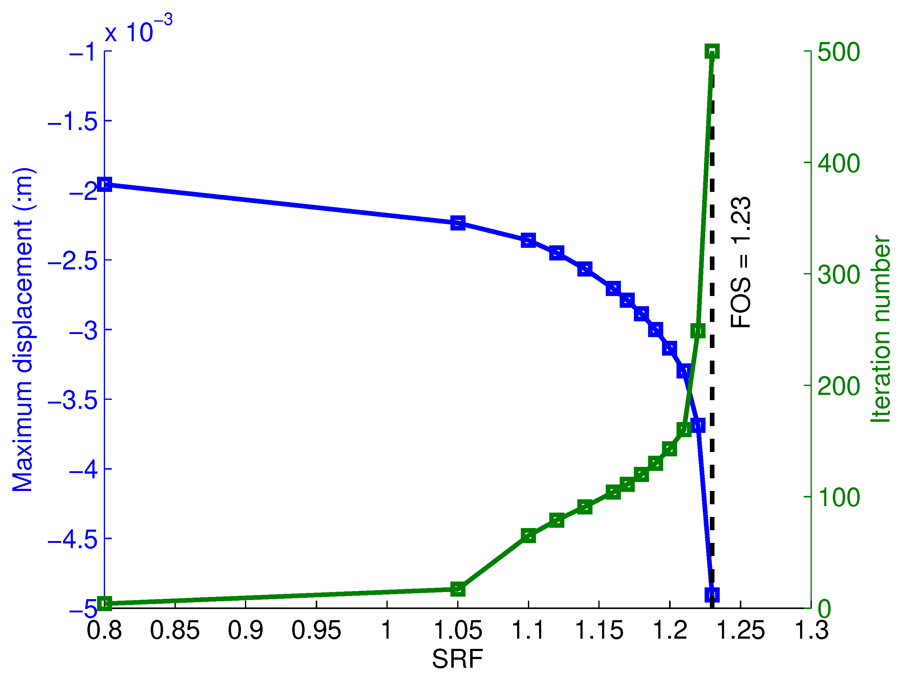
As the strength reduction method comprises an integral part of the RFEM, it is now briefly introduced to facilitate the understanding of the following auto-search algorithms and the later comparison of the two approaches to slope reliability. In the strength reduction method [15], the factor of safety (FOS) of the slope is defined as the proportion by which and c must be reduced to cause failure with the gravity loading held constant. Gravity loads are generated first and applied to the slope in a single increment. A trial strength reduction factor (SRF) loop gradually scales down the soil strength until the algorithm fails to converge within a given iteration limit (e.g., 500). Each entry of this loop implements a different strength reduction factor SRF (usually increasing). The factored soil strength parameters that go into the elasto-plastic analysis are obtained from
where c is the cohesion and is the friction angle. Progressively larger values of the SRF factor are attempted until the algorithm hits the iteration ceiling (which also indicates a sudden increase in the nodal displacement, as shown in Figure 1), at which point the SRF is then interpreted as the factor of safety FOS, therefore .
An automatic search routine (called AutoFOS) was written to find this limiting SRF to an accuracy of 0.01, taking advantage of the pattern of progression of the iteration count with SRF [16]. The AutoFOS search routine is initialised by first defining a starting SRF, and the step size to the next trial SRF value, (where superscript refers to the initial step). Three other artificial iteration cut values (Cut1, Cut2 and Cut3) are used when the iteration counts are close to failure, at which point is truncated in a prescribed manner (i.e., a larger step was taken for smaller counts and a smaller step size for larger counts, as shown in Figure 1).
The pseudocode for the AutoFOS procedure is as follows (I and C are the actual and maximum-allowed/ceiling plastic iteration counts):
******************************block 0****************************
10 Generate a slope and shear strength profile with mean,
20 Do While ( < C), j is loop number:
30 If () then ,
40 Else If () then
50 Else If () then
60 If ( < ) then
70 Else If ( > ) then
80 Else If ( > ) then
90 Else If ( > ) then
100 Else If ( > C) then Slope failed, finish
110 End If
120 End If
130 Calculate new :
140 Reduce the shear strength:
150 Finite element plastic analysis of the slope, recording the number of iterations () taken to converge
160 End Do
******************************block 0****************************
In the above and in the following, represents, in general, the mean of c and . For an undrained analysis, it represents the mean of the undrained shear strength .
3. The Random Finite Element Method
The random finite element method (RFEM) is often used to compute geotechnical structure (e.g., slope) response (e.g., factor of safety and displacements) within a Monte Carlo framework [7]. The procedure is as follows.
- Generate random property fields, for example, using the local average subdivision (LAS) method [17], based on some soil property statistics, e.g., a distribution type such as normal or lognormal characterised by the mean and standard deviation; spatial correlation structure (type of correlation function; and horizontal and vertical scales of fluctuation, and , respectively).
- Map random field cell values onto the Gauss points within the finite element mesh modelling the given problem (in this case, a slope stability problem).
- Carry out a traditional finite element (e.g., slope stability) analysis [15].
- Repeat the above steps for multiple realisations in a Monte Carlo analysis, until the output statistics (e.g., the mean and standard deviation of the factor of safety) converge.
For a given set of statistics, a probability distribution of the factor of safety can be obtained. Moreover, the potential consequences (e.g., failure volume in the case of slope stability) may also be quantified for each realised factor of safety.
An existing LAS program, implemented in [18] and improved in [19], has been used in this paper. The implementation uses the following covariance function,
where and are the lag distance and scale of fluctuation, respectively; subscripts 1–2 denote the lateral and vertical coordinate directions, respectively; and is the variance of the relevant soil property. However, because the subdivision algorithm itself is incapable of preserving anisotropy [20], in this implementation, an isotropic random field is initially generated, and this field is then postprocessed to give the target anisotropic random field; that is, by squashing and/or stretching the field in the vertical and/or horizontal directions, respectively.
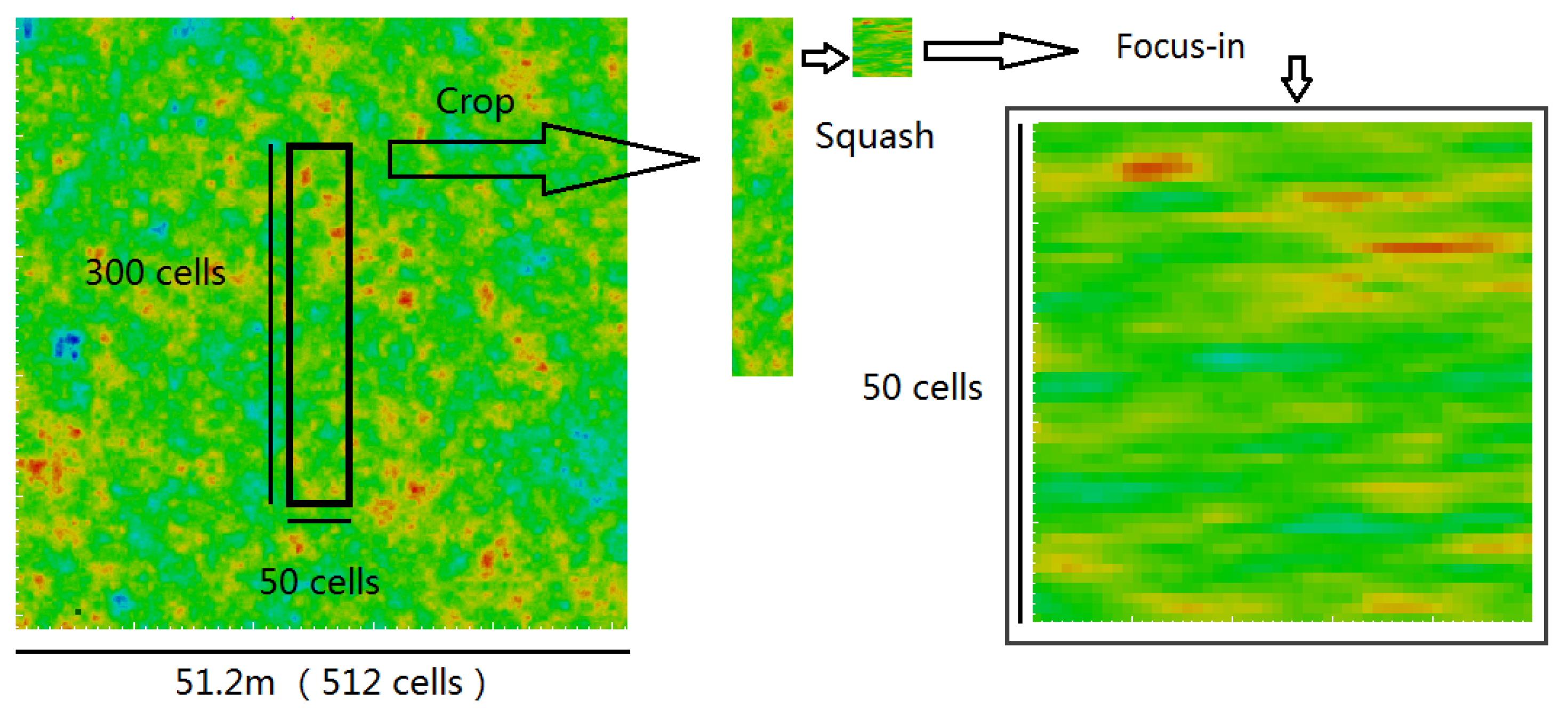
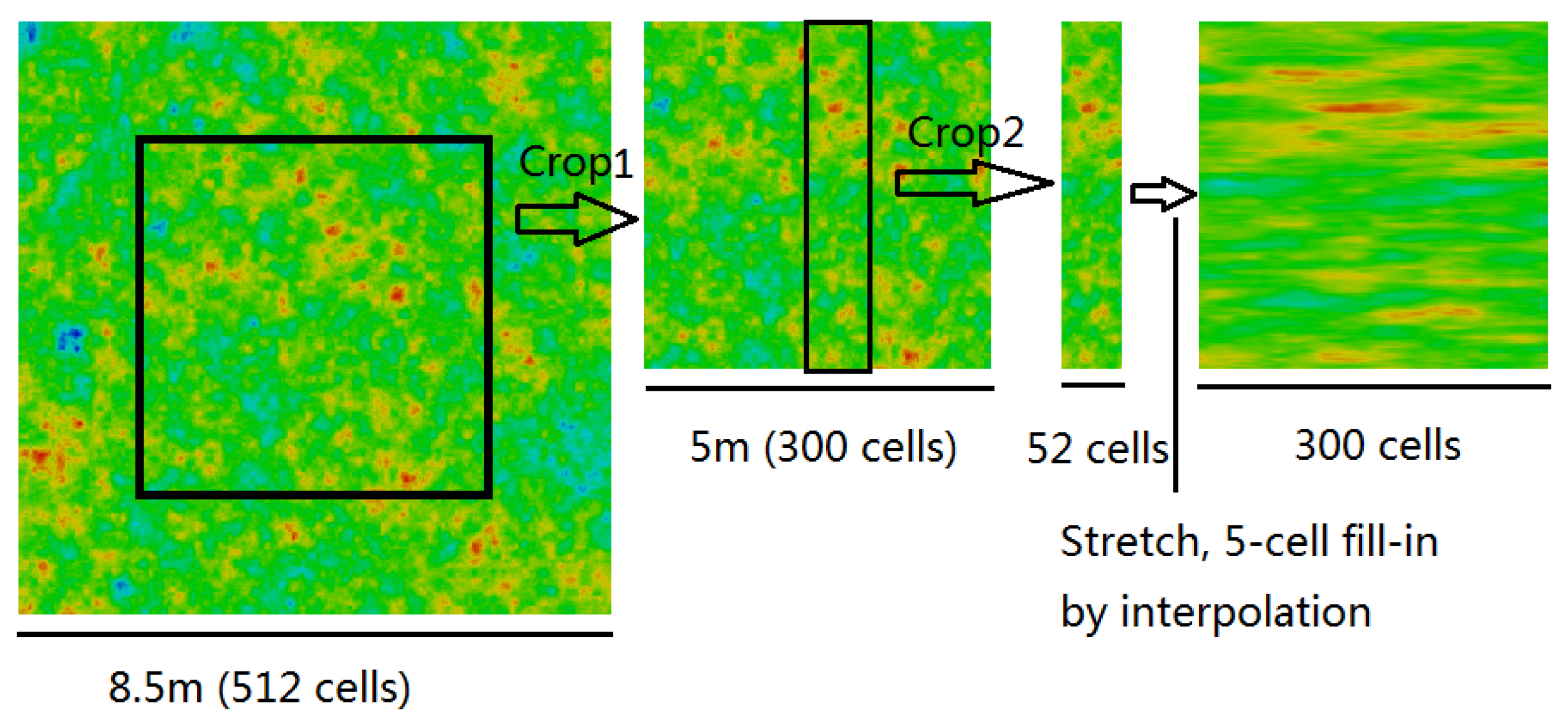
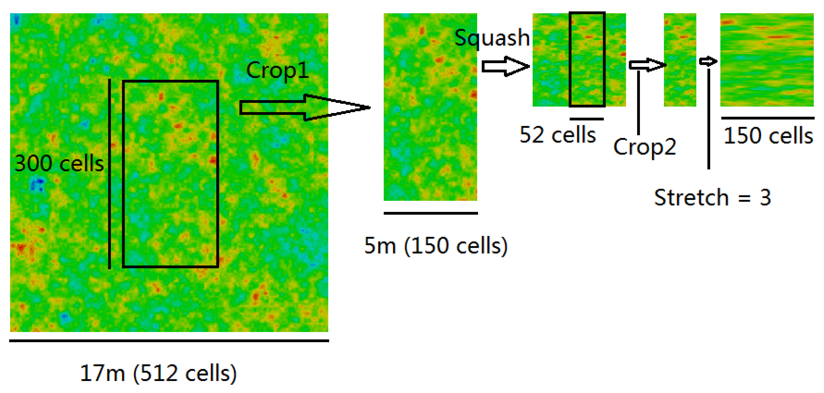
Figure 2, Figure 3 and Figure 4 show three possible ways of postprocessing an isotropic random field to produce an anisotropic field ready for mapping to a finite element mesh. In each figure, the starting point is an isotropic random field comprising 512 × 512 cells (i.e., as has been generated by nine LAS subdivision stages).
Figure 2 shows an example of squashing the starting isotropic random field vertically. In this example, the target square domain size is m, the vertical scale of fluctuation is m, and the anisotropy of the heterogeneity is , i.e., the horizontal scale of fluctuation is m. The final cell size is 0.1 m, and therefore 50 cells are needed in the horizontal direction and cells (before squashing) in the vertical direction, as these are to be squashed and replaced by 50 new square cells. The starting isotropic field has a scale of fluctuation of m, to ensure that the final target field has the required horizontal and vertical SOFs. Note that, by squashing vertically (and averaging each group of 6 cells to form a single new cell of 0.1 m dimension), the vertical scale of fluctuation is scaled down to the target 0.5 m.
The same target field can also be produced by stretching an isotropic random field with m, as illustrated in Figure 3. In this example, the horizontal SOF is scaled up to 3.0 m and so each of the original square cells needs to be replaced by six new square cells (each with their own cell value). The extra cell values can be assigned by linear interpolation between neighbouring columns of cells in the original field [16], as illustrated in Figure 3. Note that the original field before cropping is exactly the same as the original field from Figure 2, due to the different random field cell sizes. Here, the cell size is 1/60 m, i.e., by keeping the ratio the same as in Figure 2, to ensure the same amount of variance reduction at the “point” level.
Squashing and stretching may also be combined to give the target field. For example, the same target field as shown in Figure 2 and Figure 3 can be produced by first squashing by a factor of 2 from an isotropic field having m (Figure 4). After squashing, the intermediate field has a vertical SOF of m and a horizontal SOF of m. Therefore, by stretching the squashed field horizontally by a factor of 3, the resultant field will have a horizontal SOF of m. Note that, to make the variance reduction in the final field consistent with the above figures, the cell size here is set to 1/30 m, so that is the same as above.
4. Quantitative Consequence Assessment of Slope Failures
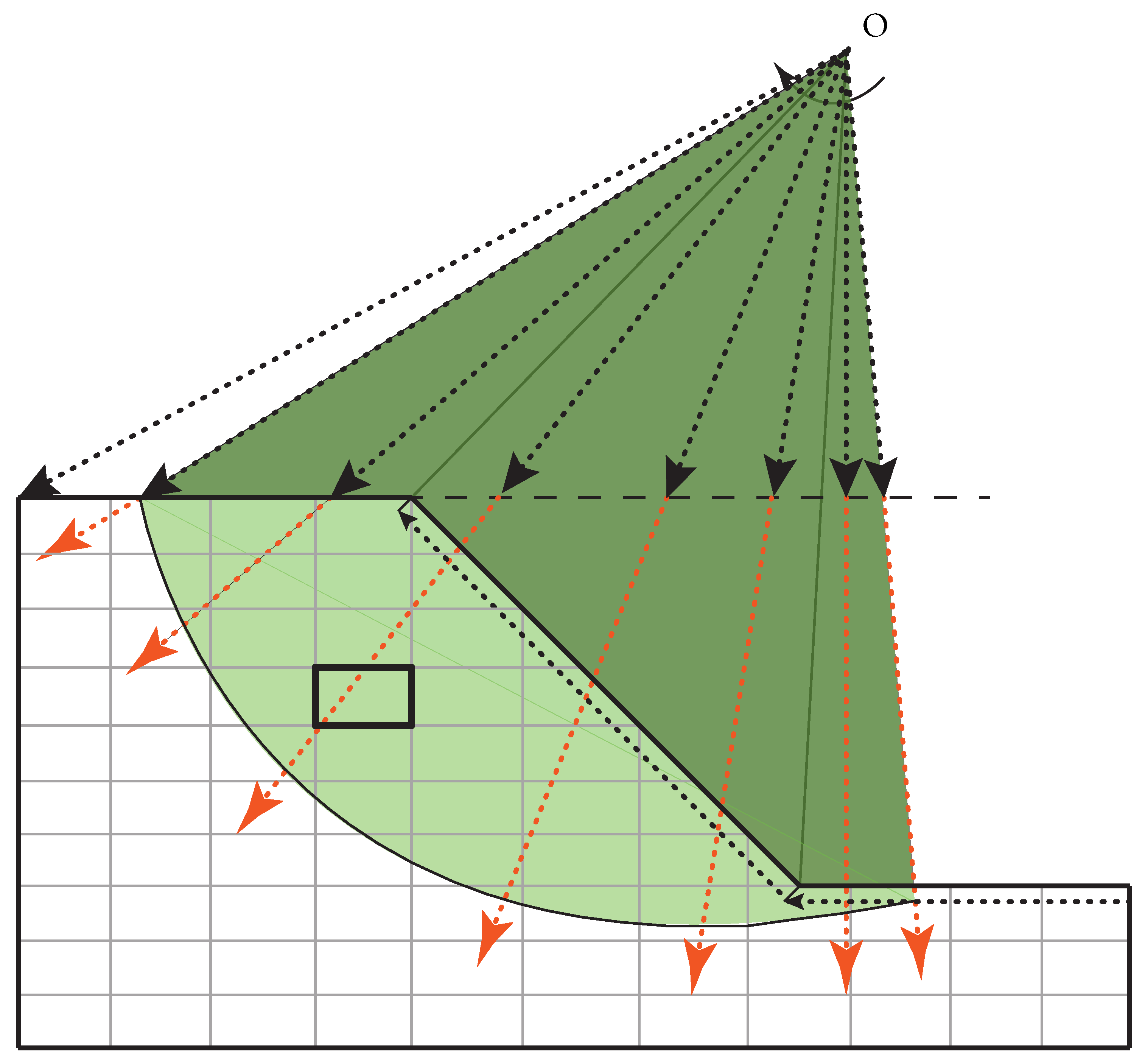
Radiating Scan Method
As the sliding volumes will be used later to explain the differences of the two approaches, a procedure called the radiating scan method is proposed and briefly introduced here. To quantify the failure volume, an estimation of slip area (A) has to be made for the problem. This is done by locating the rupture surface first, then smoothing this surface and at last, finding the arc length () and A by integration.
The technique used in [21] has been adopted to define the rupture surface based on the shear strain invariant,
in which , and are the normal strains in the x and y directions and shear strain, respectively.
First, the maximum shear strain invariant was found along the line just below the toe and the line just below the slope face. Next, an imaginary point in space, above the centre of the slope face, was chosen. Then, a series of lines radiating out from this point (across the slope mesh, clockwise) was considered (the first radiating line is the line connecting the point located in the first step and the imaginary point). The maximum value of shear strain invariant along each line (i.e., clockwise) was detected and, by connecting the locus of maxima from all the lines, the rupture surface was defined. This is shown in Figure 5 schematically. Note that the shear strain invariant within an element is interpolated using the shape functions.
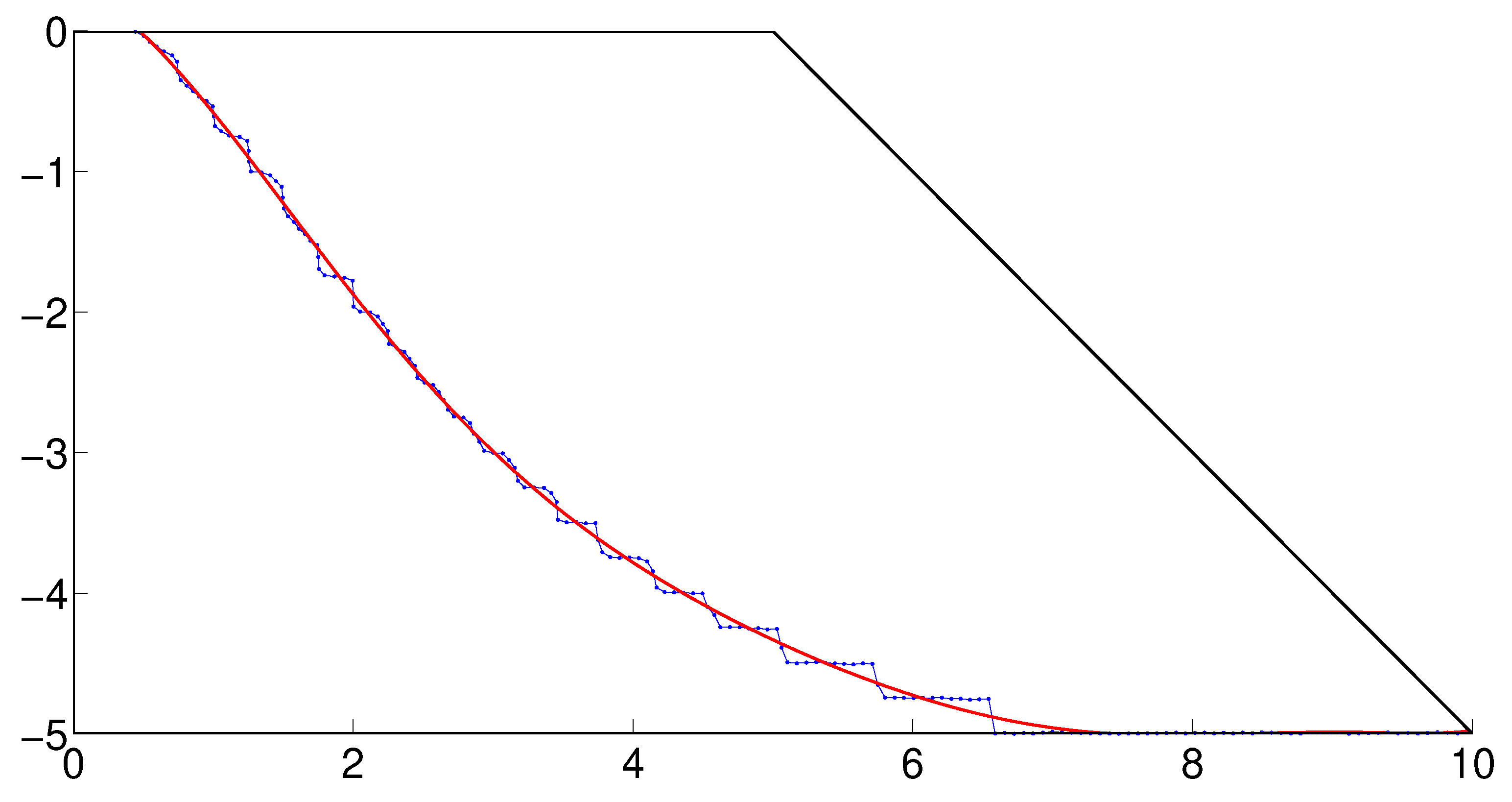
However, no precise information about the length of the rupture surface is available by adopting the above-mentioned Radiation Scan method only. A procedure is implemented to smooth the curve by polynomial curve fitting; that is, by finding the coefficients of a polynomial of degree n that fits the data, to , in a least squares sense, () are the coordinate pair defining the rupture surface). By doing so, the rippled curve shown in Figure 6 is smoothed to the curve shown in red. Next, the arc length is found by numerically integrating between 0.5 and 10:
Figure 6 shows that the slip area is found by computing the integral of p with respect to x, using repeated trapezium integration and then subtracting the area of the triangle above the slope face. For the present slope geometry and failure mechanism, the integrated length of the rupture surface is m and the slip area is m2.
5. Slope Reliability Assessment—The Two Approaches
5.1. Definitions of Factor of Safety
There are two definitions for the factor of safety: The first uses as a ratio of absolute strength (structural capacity) to actual applied load; this is a measure of a particular design (i.e., for a particular realisation from a Monte Carlo simulation). The other uses of factor of safety, which is a constant value imposed by law, standard/code, specification, contract or custom to which a structure must conform or exceed. As the definition is sometimes confusing, it is important to be aware of which definition(s) are being used.
- Realized factor of safety, : This is a calculated value from a specific realisation of a Monte Carlo simulation. For different realisations from the same set of statistics (), this value may be different as per realisation. Typically, there is a range of values following some distributions for this type of FOS.
- Traditional factor of safety, , based on the mean property value: This is the factor of safety (a required value) as a design factor. This FOS is traditionally defined in a deterministic point of view, i.e., in traditional mechanics, as the ratio of mean strength to mean applied load.
In a RFEM analysis, each traditional is associated with some reliability level ( indicates failure, and stable otherwise). In other words, there may be a range of realised for each target traditional for which those values of may be larger or smaller than , due to different realisations (which is unknown because of limited site investigation) of the spatial variability of soil strength properties.
5.2. Approach I
The approach will be explained in the case of an undrained clay slope characterised by the spatially variable undrained shear strength .
The mean (i.e., ) of for , based on deterministic finite element analysis (FEA), is found first. Next, using this value of (e.g., kPa for the slope analysed in Figure 6) and the corresponding values of and , the distribution in the slope is generated (note that, due to the relative positioning of weak and strong zones in the slope, the realised could be larger or smaller than 1.0). The values (for the realisation generated in the last step) are then scaled up by progressively larger values of , and, for each value of , the slope is analysed to see if it is stable (i.e., the FEA is conducted only for one trial SRF = 1.0, if the plastic iteration count reaches 500, then the slope fails; that is . The algorithm does not try to find the exact ; it could be any value smaller than 1.0 if the slope failed). By repeating this process for a large number of realisations (N) while counting the number of failed slopes () for each , the reliability of the slope may be computed for a range of values of , thereby resulting in a reliability versus curve.
Note that if the FEA converges within iterations (i.e., less than 500) with a trial SRF = 1.0, then it means that the realised for that realisation must be larger than 1.0 (i.e., an SRF larger than 1.0 is needed to allow the plastic algorithm to hit the 500 iteration ceiling); that is, the slope is stable for that that is used to scale up that realisation.
The pseudocode for approach I is as follows ( is the plastic iteration count):
******************************block 1****************************
10 Initialisation: and input
20 For N realisations (loop i):
30 Generate a slope and shear strength profile () with ;
40 For a series of values of
(e.g., with ) (loop j):
50 Scale up profile by
60 Carry out FEA, let , if , then
70 Output: for each
******************************block 1****************************
or alternatively,
******************************block 2****************************
10 Initialisation: and input
20 For a series of values of
(e.g., with ) (loop j):
30 For N realisations (loop i):
40 Generate a slope and shear strength profile () with ;
50 Scale up profile by
60 Carry out FEA, let , if , then
70 Output: for each
******************************block 2****************************
The algorithm presented in block 2 is not efficient compared to that shown in block 1 as line 30 needs to be regenerated for each considered.
The probability of failure, , for a given , is
in which N is the total number of realisations and (in which superscript 1 denotes the approach I) is the number of realisations in which slope failure has occurred (i.e., ).
5.3. Approach II
The (i.e., undrained shear strength) distribution in the slope is generated, based on the statistics (i.e., mean , variance and scales of fluctuation ) of . The factor of safety for each realisation of the slope is then found by scaling down the values of by progressively larger values of strength reduction factor (SRF), until the limiting value of SRF (i.e., the realised ) is obtained. This process is repeated for a large number of realisations, to obtain a distribution of .
The pseudocode for approach II is as follows:
******************************block 3****************************
10 Input statistics corresponding to
20 For N realisations (loop k):
30 Generate a slope and shear strength profile () with ;
40 Carry out FEA using progressively larger SRF, if , then
50 Output: a distribution of
******************************block 3****************************
Note the similarity of block 3 to block 2; block 3 has one input and tries to find the whole distribution of for all realisations, whereas block 2 works on a series values of and does not try to find the exact for all realisations (only to see if it is stable or not).
Now, define a unified factor as
Note that, for a particular realisation, if is proportional to (or any other value ) by a factor of (or ), the realised is also propotional to (or ) by the same factor. This is because, whether one starts the strength reduction process (to get the realised factor of safety for that realisation) from a high mean shear strength (high ) or a low mean shear strength (low ), in both cases the slope falls down when the mean strength along the failure surface reaches the same critical value (for the same spatial variation of soil properties). For example, if and for a particular realisation (the critical value of strength is then , where is the random cell values along the failure path, generated based on , and f is a function that determines the mean strength along the failure path); then, for the case of , to reach the same critical value, the realised must be . In this case, . For multiple realisations, the same holds.
The probability of failure, , at a given , is
in which N is the total number of realisations and (in which superscript 2 denotes the approach II) is the number of realisations in which slope failure has occurred (i.e., ).
The failure is defined as a slope failed at for any , e.g., . Upon transformation to (Equation (6)), the definition of slope failure is preserved by defining as failure (i.e., when in Equation (6), ).
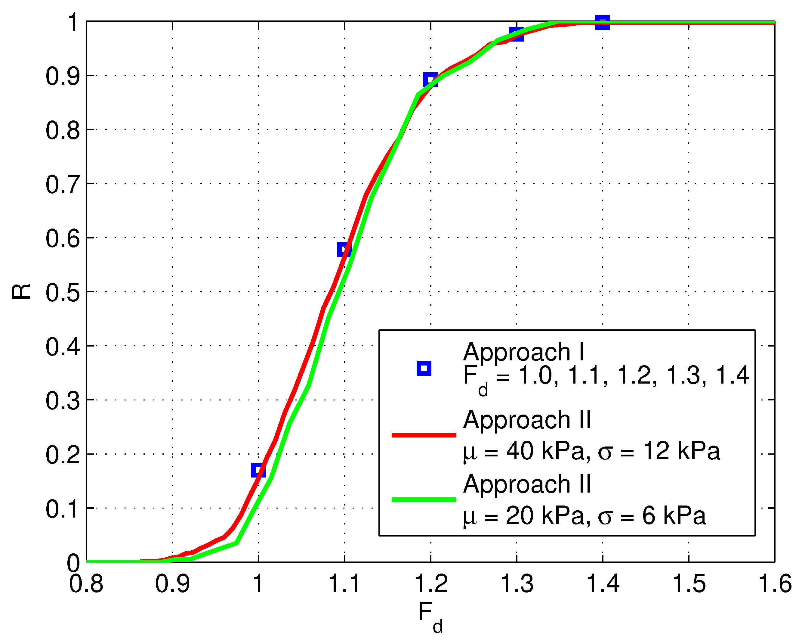
As shown in Figure 7, an analysis based on kPa and kPa () gives virtually the same results as the analysis based on kPa and kPa (), where . The slight difference is due to the different settings (initial FOS, initial FOS step and the three cut values of plastic iteration counts) for the AutoFOS implementation.
Note that it does not matter whether the input statistics are kPa and kPa () or kPa and kPa ( = 1.23). Therefore, for , the transformed outputs (the subscript i denotes “identical”) are the same, based on Equation (6), if the initial seed for generating the random field is identical (thereby the relative strong and weak spatial distribution of soil properties in the individual realisation of random field is the same for the two cases, only the random field cell values differ by a factor of 2).
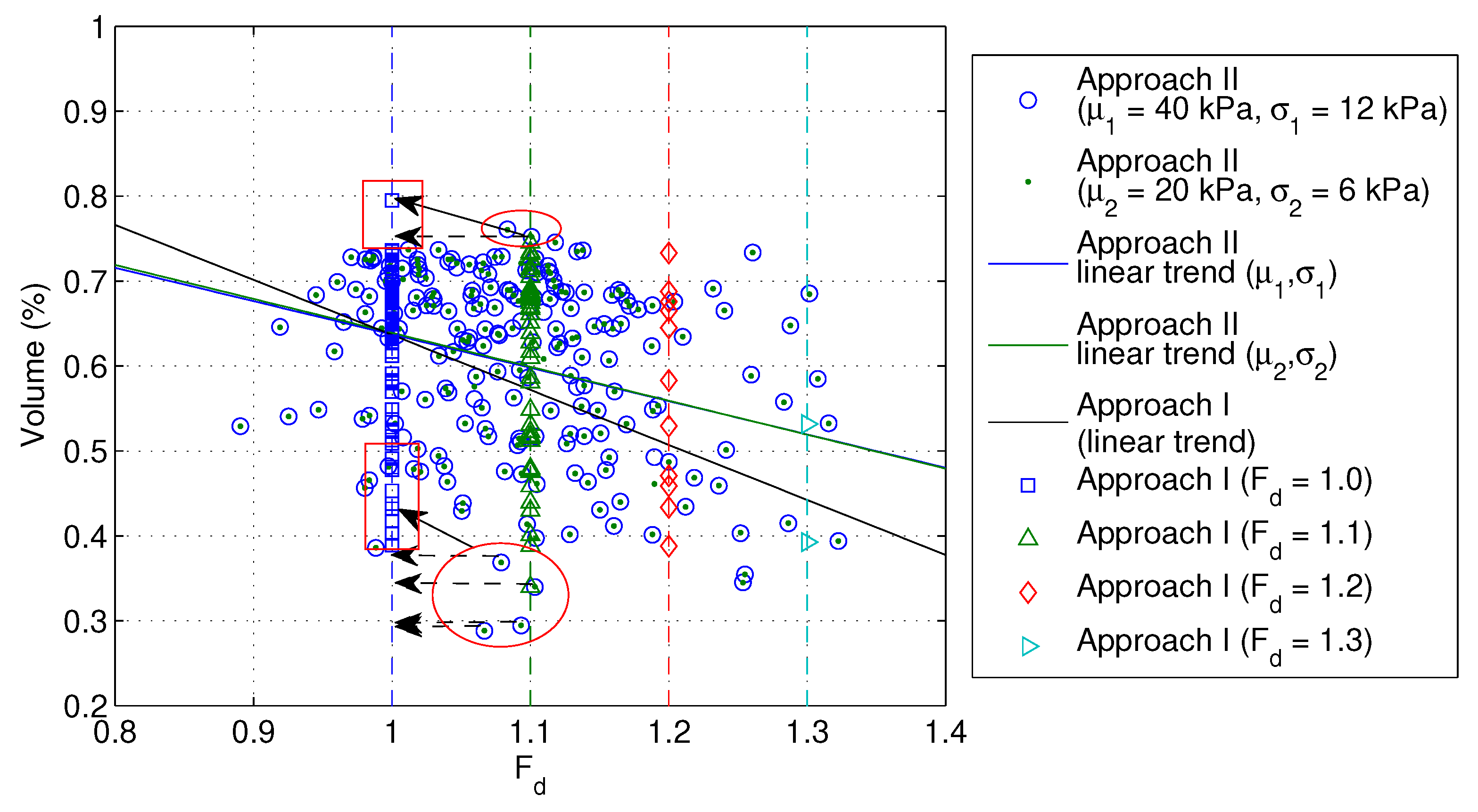
This is clearly shown in Figure 8, where an analysis based on 40 kPa and 12 kPa gives the same failure volumes as those for an analysis based on 20 kPa and 6 kPa, as indicated by the points sitting in the centre of the circles.
The results of analyses based on Approach I with different sets of inputs (Table 1) are also shown in Figure 7. They are in good agreement with the results of Approach II. For each set of input, if the analysis were done in the same way as Approach II to get the whole distribution of , the fitted curve would be similar to those shown in Figure 9 (not necessarily the same, because those curves are based on hypothetically generated random numbers).
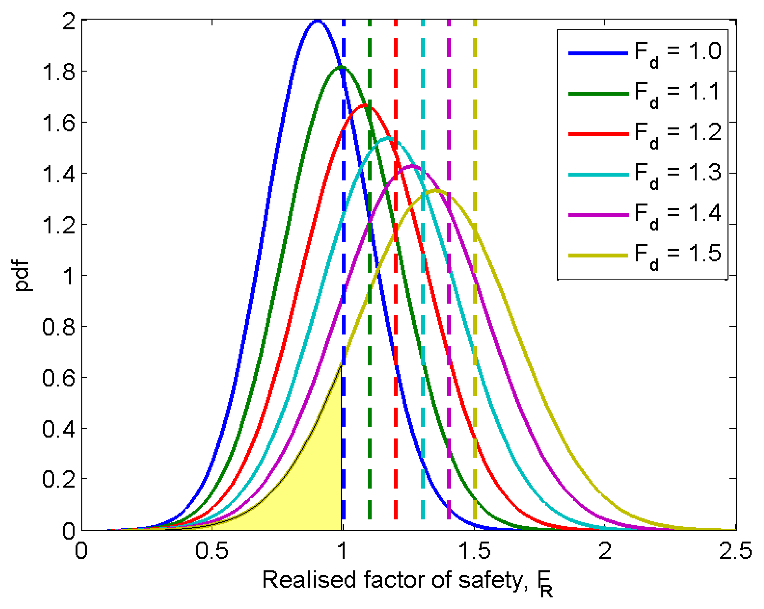
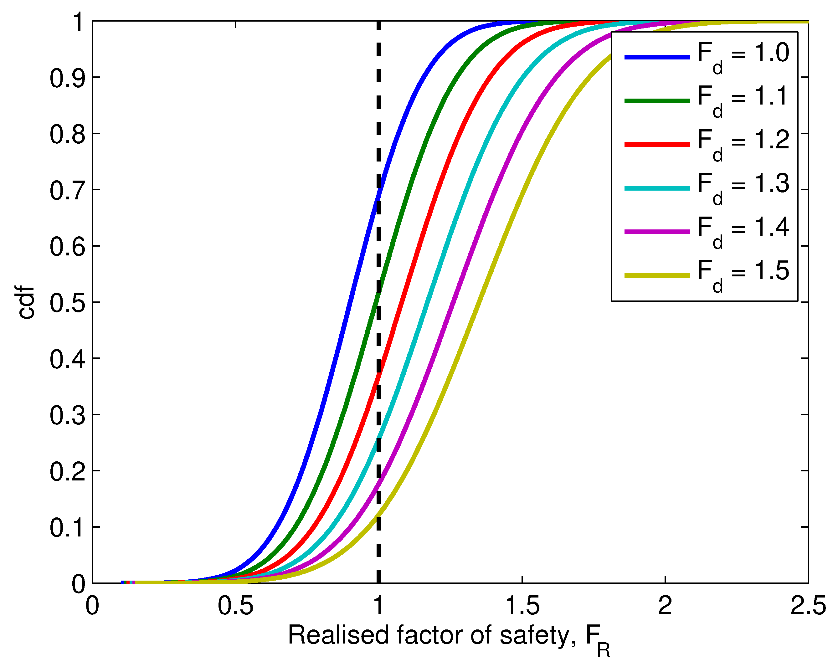
Figure 9 shows the changing of probability of failure as increases, as represented by the areas under the corresponding pdf curves to the left of 1.0 (the probability of failure can also be read directly from the cdf curves shown in Figure 10). Those curves represent the fitted curves of the realised . The curve corresponding to is hypothetically created based on a mean of 0.9 and a standard deviation of 0.2 (that is, and ; note that the value of is assumed here to represent a smaller mean than that was observed in a typical RFEM analysis), and those corresponding to 1.1, 1.2, 1.3, 1.4 and 1.5 are created by scaling up the for by factors of , , , and , respectively (cf. Equation (6)). By doing so, and , for various , are also scaled up by the same factors. Therefore, the relative position of and does not change; this is in accordance with Equation (6).
5.4. Equivalence and Differences between the Two Approaches
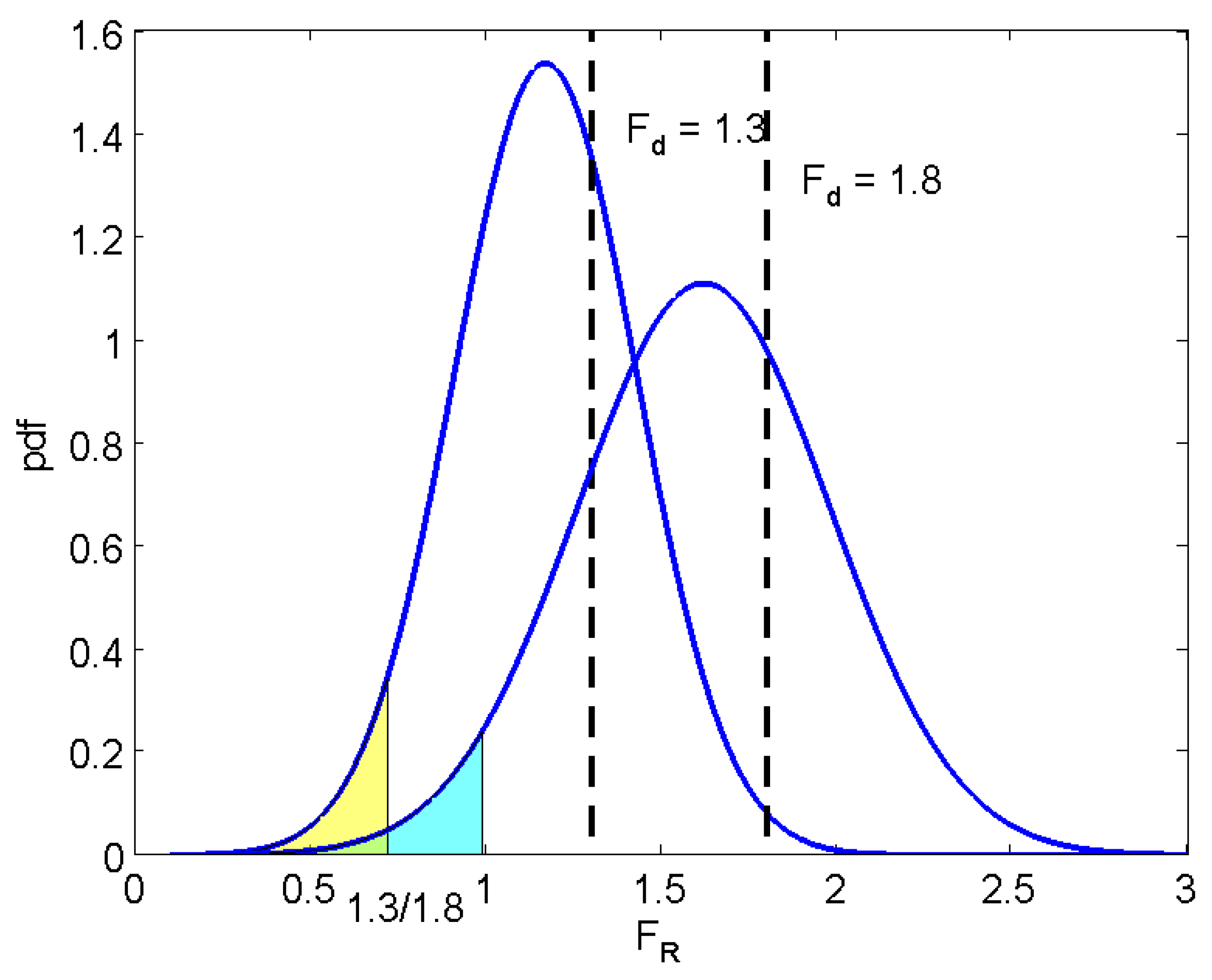
In essence, these two methods are equivalent to each other. Approach II is a unified approach, regardless of the specific input provided that COV is constant. This can be explained by Equation (6). In fact, once a distribution of is obtained from a base case, for example, , the distributions of for other values (i.e., any value) of can be inferred. This is shown in Figure 11. Not only the distribution can be inferred, but also the probability of failure for any . As shown in Figure 11, the shaded area below the pdf to the left side of 1.0, for a given , is equal to the shaded area below the pdf to the left side of . The reason behind this lies in the following expression of the cumulative distribution function of a normal distribution,
where is the error function.
Based on the above equation, and by setting and changing the values of and for any given series of values of (which is proportional to the value of and for the base case ), the reliability versus curve can be obtained; this is essentially Approach I.
The same results can be obtained by only looking at the distribution of for the base case. That is, in Equation (8), let and be the values based on the base case, and change the value of to be . This way, the reliability versus curve can also be obtained; this is essentially Approach II.
Note that the series of values can be any prescribed values, for example, . In a typical RFEM simulation, one can either prescribe a series of values or by simply taking the values of from the base case and using them as the series of values (or take the values of (Equation (6)) as the prescribed ).
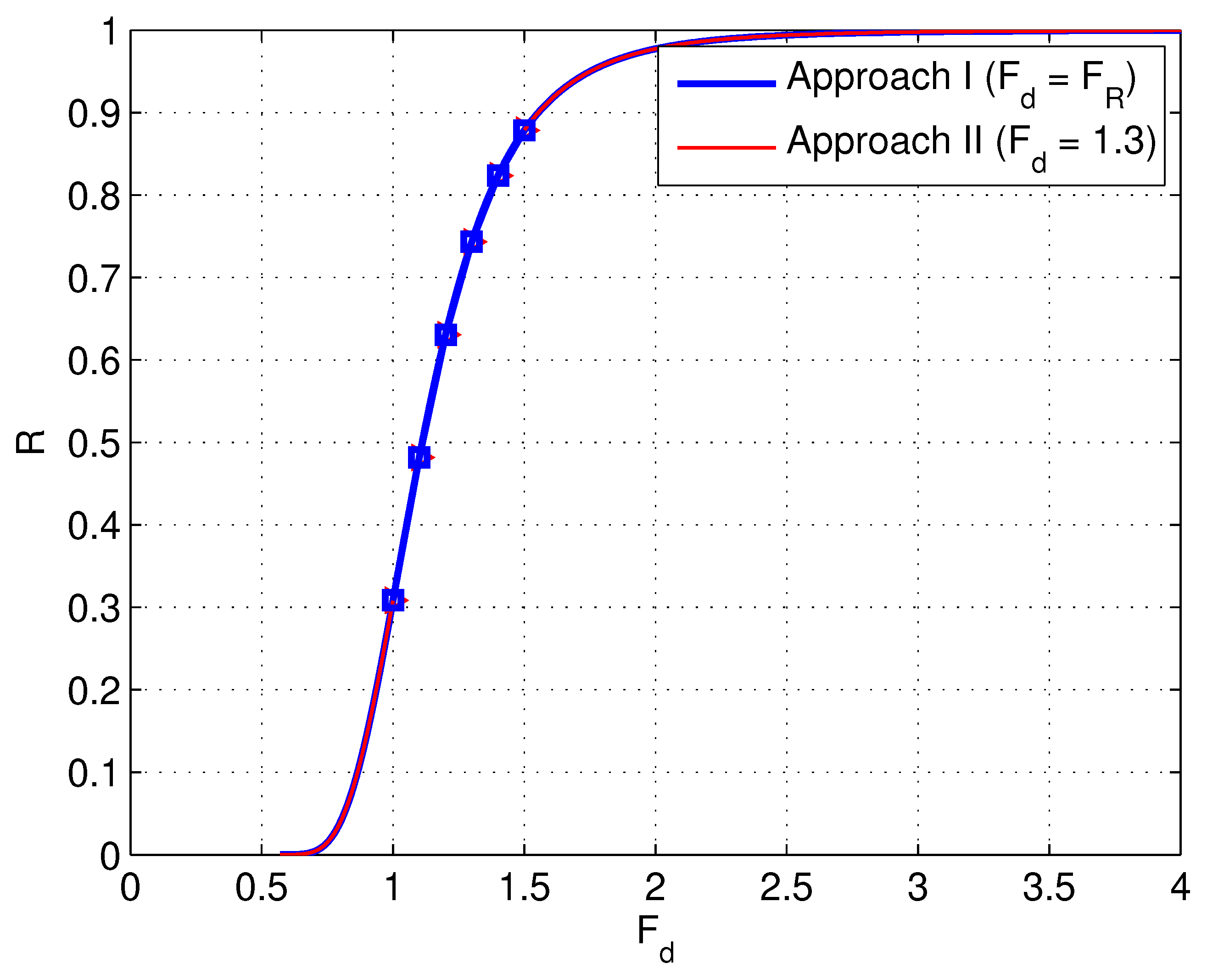
The results from the base case of ( and ) is shown in Figure 12 for the two cases: (1) when prescribing (the discrete points in the figure); (2) when prescribing (i.e., the series of values of from the base case).
For approach I, if the slope fails for a trial factor (SRF) of 1.0, the realised could be some value smaller than 1.0. For instance, if the plastic iteration count reaches the limit for SRF = 1.0, it might have reached the limit for SRF = 0.9, or some value that is smaller than 1.0. However, it did not really get the for those realisations that fail (). They were assumed to be 1.0, consequently, was assumed to be (Equation (6)). Actually, this is better illustrated in Figure 8. With Approach I, the figure is plotted by pulling back these points sitting to the right of the vertical lines of and . The calculated reliability is identical for the two approaches. That is, for each given , the probability of failure is the ratio of the number of points (realisations) sitting to the right of this, , to the total number of points (realisations) in Figure 8. Note that the points in any vertical line comprise all the projective points (from the base case in Approach II) sitting to the right of that line. So, if the increment of is fine enough, e.g., or , instead of the previously used , the figure plotted using Approach I (that is, in terms of vertical lines, excluding the realisations or points that have already failed for larger under consideration, and only including these new failed realisations or points) would be the same as that produced by Approach II.
The linear trend for failure volumes shown in Figure 8 indicates that the volumes are smaller for higher [21]. As increases or the probability of failure decreases (Figure 7), the potential slide volumes becomes smaller. In other words, the risk associated with a higher global factor of safety () may be relatively low, due to the low probability of failure and a decreased likelihood of large slide volumes (or an increased trend of small slide volumes). However, it will be shown that Approach I may result in underestimated sliding volumes at low failure probability levels and thereby underestimated risk (i.e., unconservative).
Note that with Approach I, the slopes that have failed for larger will definitely fail for small (the possibility of improving the code efficiency arises for code blocks 1 and 2, i.e., by letting the series of values of starts with a larger value and gradually decreases by some step size, this way those realisations that have failed for a larger would not be needed to be analysed for any smaller ). Because of this, the failure mechanisms for the same realisations will be more thoroughly formed for small compared to those for larger , and tend to be deeper. Thus, larger volumes are usually detected, as illustrated in Figure 8 by the up-shifted points that should be projected horizontally to the line to their left side (the arrows in dotted lines show the positions that the relevant points should be projected to, and the solid arrows show the actual positions to which these points are projected). However, the effect of these up-shifted volumes on the distribution and range of possible failure volumes are unknown and difficult to clarify. This effect tends to increase the number of shifted volumes as decreases. The worst consequence would be that part of the linear trend could possibly be attributed to the up-shifting when adopting Approach I (see the deviated trend in Figure 8). After scrutiny, it was found that most of the realisations have the same rupture surfaces as those detected for larger . As shown in Figure 8, for , which is the worst case, only eight realisations have had significantly different slide volumes compared to those for (those realisations are 7, 20, 57, 60, 71, 76, 84, 97). This was thought to be due to the nested failure mechanisms for those realisations. Anyway, this is an integral part of the implementation of Approach I (i.e., for those slopes failed for the largest considered, SRF = 1.0 is the trial factor; these slopes will definitely fail for smaller under consideration, the trial factor is still 1.0, whereas a trial factor of, say, 0.9 would give the same failure extent). No effort was taken to improve this, as more time would be demanded to locate the actual limiting SRF (some value less than 1.0) for those known failures.
Due to the up-shifting effect and the necessity to refine to get a smooth reliability curve, the implementation of Approach I is thought to be a bad choice, although the calculation time might be an advantage (i.e., there is no need to search for the whole distribution of realised for each considered. However, if refined, this advantage could be counterbalanced). The implementation of Approach II is preferable, in that the volumes are distributed over the whole region for each , a whole distribution of realised can be gained and the reliability curve is smoother.
It is noted that the above is presented based on a normal distribution assumption of shear strength and thus (Equation (8)). For a lognormal distribution of shear strength, and thus a lognormal distribution of , the cumulative distribution function of is
where is the error function.
In the case of a lognormal distribution of strength, the target log-normal random field can be represented by
where is a normal random field given by
where is a standard normal random field with zero mean and unit variance and and are given by
Assume that for a particular and a series of is obtained based on this , this is referred to as the base case. For a target , i.e., any given target value, the values need to be scaled by a factor of . For a constant coefficient of variation , and , it follows that . In turn, . Therefore, the series of for the base case can also be scaled by the same factor to give the values for the target .
Similar to the normal case, the probability of failure can be assessed by setting in Equation (9), i.e.,
By changing and for various values of , the reliability (i.e., ) can be assessed.
On the other hand,
where the derivation makes use of the generic form of Equation (12), i.e., for .
That is, the reliability (i.e., ) can be assessed by letting in Equation (9) and keeping and as the values based on the base case. Therefore, the conclusions in this paper can be considered general for the two most commonly used distribution types, i.e., normal and lognormal distribution.
6. Conclusions
This paper focuses on the two approaches in RFEM assessments of slope reliability. A comprehensive analysis was conducted to explain the often confusing methods of analysis. Some researchers use one approach while others use the other and it is difficult to understand the second approach (e.g., how the scaling works) and even more so to link to the first approach in some cases.
Based on an auto-search algorithm of the factor of safety in the strength reduction method, and a radiation scan method to locate the critical sliding surface and to quantify the potential sliding volume, the paper demonstrates that the two approaches are actually equivalent and bridges the gap in understanding the two approaches that are usually used by different researchers in isolation.
The merits and disadvantages of each approach are highlighted. The unification where the two approaches meet is explained. That is, for a sufficiently small step size of the global factor of safety, the results of approach I are moving close to those of approach II, which are smooth for a sufficiently large number of realisations. However, when the step size becomes small, the advantage of Approach I being computationally efficient is compromised. Efficient implementations of both approaches are provided in the form of pseudocodes, as different combinations of parameters are usually required such as different coefficients of variation and different site spatial variability scenarios represented by different scales of fluctuation.
Although the investigations and discussions are presented mainly in the case of a normal distribution of the realised factor of safety, the applicability of the underlying reasoning is also extended to a log-normal distribution of the realised factor of safety.
Note that the reason of using a range of global factor of safety, (i.e., corresponding to different mean soil properties), for the two approaches, is not because the mean soil property is a variable for a particular site, as it is not. Rather, it is meant for a range of characteristic values to be used for design, which could vary from designer to designer. That is, different designers may use different to get their characteristic values.
Author Contributions
Conceptualisation, Y.L.; methodology, Y.L.; software, Y.L.; validation, C.Q., Y.L. and Z.F.; formal analysis, C.Q.; investigation, Y.L.; resources, Z.F.; data curation, Z.L.; writing—original draft preparation, Y.L.; writing—review and editing, Z.F.; visualisation, Z.L.; supervision, Y.L.; project administration, Y.L.; funding acquisition, Y.L.
Funding
This research was funded by the National Natural Science Foundation of China, grant number 41807228; the Fundamental Research Funds for the Central Universities, grant number 2652017071; and the Open Foundation of Key Laboratory of Failure Mechanism and Safety Control Techniques of Earth–Rock Dam of the Ministry of Water Resources, grant number YK319004. The last author appreciates the supports of the National Key R&D Program of China (2017YFC0405104) and the National Natural Science Foundation of China (51979173).
Conflicts of Interest
The authors declare no conflicts of interest.
Abbreviations
The following abbreviations are used in this manuscript:
| RFEM | Random finite element method |
| FOS | Factor of safety |
| SRF | Strength reduction factor |
| LAS | Local average subdivision |
| FEA | Finite element analysis |
| probability density function | |
| cdf | cumulative distribution function |
References
- Duncan, J.M. Factors of safety and reliability in geotechnical engineering. J. Geotech. Geoenviron. Eng. 2000, 126, 307–316. [Google Scholar] [CrossRef]
- Nguyen, V.U.; Chowdhury, R.N. Probabilistic study of spoil pile stability in strip coal mines—Two techniques compared. Int. J. Rock Mech. Min. Sci. Geomech. Abstr. 1984, 21, 303–312. [Google Scholar] [CrossRef]
- Fenton, G.A.; Griffiths, D.V.; Urquhart, A. A slope stability model for spatially random soils. In Proceedings of the 9th International Conference on Applications of Statistics and Probability in Civil Engineering, San Francisco, CA, USA, 6–9 July 2003; pp. 1263–1269. [Google Scholar]
- Griffiths, D.V.; Huang, J.; Fenton, G.A. Influence of spatial variability on slope reliability using 2-D random fields. J. Geotech. Geoenviron. Eng. 2009, 135, 1367–1378. [Google Scholar] [CrossRef]
- Hicks, M.A.; Samy, K. Influence of heterogeneity on undrained clay slope stability. Q. J. Eng. Geol. Hydrogeol. 2002, 35, 41–49. [Google Scholar] [CrossRef]
- Hicks, M.A.; Onisiphorou, C. Stochastic evaluation of static liquefaction in a predominantly dilative sand fill. Géotechnique 2005, 55, 123–133. [Google Scholar] [CrossRef]
- Fenton, G.A.; Griffiths, D.V. Risk Assessment in Geotechnical Engineering; John Wiley & Sons: New York, NY, USA, 2008. [Google Scholar]
- Hicks, M.A.; Spencer, W.A. Influence of heterogeneity on the reliability and failure of a long 3D slope. Comput. Geotech. 2010, 37, 948–955. [Google Scholar] [CrossRef]
- Hicks, M.A.; Nuttall, J.D.; Chen, J. Influence of heterogeneity on 3D slope reliability and failure consequence. Comput. Geotech. 2014, 61, 198–208. [Google Scholar] [CrossRef]
- Li, Y.J.; Hicks, M.A.; Nuttall, J.D. Comparative analyses of slope reliability in 3D. Eng. Geol. 2015, 196, 12–23. [Google Scholar] [CrossRef]
- Li, Y.J.; Hicks, M.A.; Vardon, P.J. Uncertainty reduction and sampling efficiency in slope designs using 3D conditional random fields. Comput. Geotech. 2016, 79, 159–172. [Google Scholar] [CrossRef] [Green Version]
- Hicks, M.A.; Li, Y.J. Influence of length effect on embankment slope reliability in 3D. Int. J. Numer. Anal. Methods Geomech. 2018, 42, 891–915. [Google Scholar]
- Griffiths, D.V.; Fenton, G.A. Probabilistic slope stability analysis by finite elements. J. Geotech. Geoenviron. Eng. 2004, 130, 507–518. [Google Scholar] [CrossRef]
- Huang, J.; Lyamin, A.V.; Griffiths, D.V.; Krabbenhoft, K.; Sloan, S.W. Quantitative risk assessment of landslide by limit analysis and random fields. Comput. Geotech. 2013, 53, 60–67. [Google Scholar] [CrossRef]
- Smith, I.M.; Griffiths, D.V. Programming the Finite Element Method; John Wiley & Sons: New York, NY, USA, 2005. [Google Scholar]
- Spencer, W.A. Parallel Stochastic and Finite Element Modelling of Clay Slope Stability in 3D. Ph.D. Thesis, University of Manchester, Manchester, UK, 2007. [Google Scholar]
- Fenton, G.A.; Vanmarcke, E.H. Simulation of random fields via local average subdivision. J. Eng. Mech. 1990, 116, 1733–1749. [Google Scholar] [CrossRef]
- Samy, K. Stochastic Analysis with Finite Elements in Geotechnical Engineering. Ph.D. Thesis, University of Manchester, Manchester, UK, 2003. [Google Scholar]
- Li, Y.J. Reliability of Long Heterogeneous Slopes in 3D-Model Performance and Conditional Simulation. Ph.D. Thesis, Delft University of Technology, Delft, The Netherlands, 2017. [Google Scholar]
- Fenton, G.A. Error evaluation of three random-field generators. J. Eng. Mech. 1994, 120, 2478–2497. [Google Scholar] [CrossRef]
- Hicks, M.A.; Chen, J.; Spencer, W.A. Influence of spatial variability on 3D slope failures. In Proceedings of the 6th International Conference on Computer Simulation in Risk Analysis and Hazard Mitigation, Cephalonia, Greece, 5–7 May 2008; pp. 335–342. [Google Scholar]
Figure 1.
Strength reduction factor versus maximum displacement and iteration numbers for a 45° slope with an undrained shear strength of 20 kPa.
Figure 1.
Strength reduction factor versus maximum displacement and iteration numbers for a 45° slope with an undrained shear strength of 20 kPa.

Figure 2.
Postprocessing an isotropic random field to produce an anisotropic field by squashing ( = 6).
Figure 2.
Postprocessing an isotropic random field to produce an anisotropic field by squashing ( = 6).

Figure 3.
Postprocessing an isotropic random field to produce an anisotropic field by stretching ( = 6) (52 cells after Crop2 to be able to interpolate between the last two columns of cells).
Figure 3.
Postprocessing an isotropic random field to produce an anisotropic field by stretching ( = 6) (52 cells after Crop2 to be able to interpolate between the last two columns of cells).

Figure 4.
Postprocessing an isotropic random field to produce an anisotropic field by squashing and stretching ( = 6) (52 cells after Crop2 to be able to interpolate between the last two columns of cells).
Figure 4.
Postprocessing an isotropic random field to produce an anisotropic field by squashing and stretching ( = 6) (52 cells after Crop2 to be able to interpolate between the last two columns of cells).

Figure 5.
A Schematic illustration of the radiating scan method for locating the failure path in 2D.
Figure 5.
A Schematic illustration of the radiating scan method for locating the failure path in 2D.

Figure 6.
Polynomial curve fitting of the scanned rupture path in 2D.

Figure 7.
Comparison of Approach I and Approach II for a 45° slope ( m and m).

Figure 8.
Comparison of the two approaches in terms of potential sliding volumes.

Figure 9.
pdf of realised showing the decrease of probability of failure as increases.

Figure 10.
cdf of realised showing the decrease of probability of failure as increases.

Figure 11.
pdf with equal shaded area showing that for other (e.g., 1.8) can be inferred from one single set of inputs based on ( and ).
Figure 11.
pdf with equal shaded area showing that for other (e.g., 1.8) can be inferred from one single set of inputs based on ( and ).

Figure 12.
Reliability curves obtained from Approach I and Approach II.


Table 1.
Input datasets for Approach I.
| Statistics | |
|---|---|
| kPa, kPa | |
| kPa, kPa | |
| kPa, kPa | |
| kPa, kPa | |
| kPa, kPa |
© 2019 by the authors. Licensee MDPI, Basel, Switzerland. This article is an open access article distributed under the terms and conditions of the Creative Commons Attribution (CC BY) license (http://creativecommons.org/licenses/by/4.0/).
Share and Cite
MDPI and ACS Style
Li, Y.; Qian, C.; Fu, Z.; Li, Z. On Two Approaches to Slope Stability Reliability Assessments Using the Random Finite Element Method. Appl. Sci. 2019, 9, 4421. https://doi.org/10.3390/app9204421
AMA Style
Li Y, Qian C, Fu Z, Li Z. On Two Approaches to Slope Stability Reliability Assessments Using the Random Finite Element Method. Applied Sciences. 2019; 9(20):4421. https://doi.org/10.3390/app9204421
Chicago/Turabian StyleLi, Yajun, Cheng Qian, Zhongzhi Fu, and Zhuo Li. 2019. "On Two Approaches to Slope Stability Reliability Assessments Using the Random Finite Element Method" Applied Sciences 9, no. 20: 4421. https://doi.org/10.3390/app9204421
Note that from the first issue of 2016, this journal uses article numbers instead of page numbers. See further details here.