3D Convolutional Neural Networks for Remote Pulse Rate Measurement and Mapping from Facial Video


Laboratoire de Conception, Optimisation et Modélisation des Systèmes, LCOMS EA 7306, Université de Lorraine, 57000 Metz, France
*
Author to whom correspondence should be addressed.
Appl. Sci. 2019, 9(20), 4364; https://doi.org/10.3390/app9204364
Submission received: 31 August 2019
/
Revised: 10 October 2019
/
Accepted: 11 October 2019
/
Published: 16 October 2019
(This article belongs to the Special Issue Contactless Vital Signs Monitoring)
Abstract
:Remote pulse rate measurement from facial video has gained particular attention over the last few years. Research exhibits significant advancements and demonstrates that common video cameras correspond to reliable devices that can be employed to measure a large set of biomedical parameters without any contact with the subject. A new framework for measuring and mapping pulse rate from video is presented in this pilot study. The method, which relies on convolutional 3D networks, is fully automatic and does not require any special image preprocessing. In addition, the network ensures concurrent mapping by producing a prediction for each local group of pixels. A particular training procedure that employs only synthetic data is proposed. Preliminary results demonstrate that this convolutional 3D network can effectively extract pulse rate from video without the need for any processing of frames. The trained model was compared with other state-of-the-art methods on public data. Results exhibit significant agreement between estimated and ground-truth measurements: the root mean square error computed from pulse rate values assessed with the convolutional 3D network is equal to 8.64 bpm, which is superior to 10 bpm for the other state-of-the-art methods. The robustness of the method to natural motion and increases in performance correspond to the two main avenues that will be considered in future works.
1. Introduction
The domain of physiological signal measurement using contactless devices has gained vast attention. Research exhibits significant advancements over the last few years and demonstrates that standard video cameras are reliable devices that can be employed to measure a large set of biomedical parameters without any contact with the subject. Nevertheless, and despite important advancements, the most recent methods are still not ready to satisfy real-world applications. The main challenge consists in improving robustness to natural motion that produces undesirable noise and artifacts in the measurements. This issue is common to most systems that record and analyze images to sense vital signs and biomedical parameters. In the era of ubiquitous computing where mobile devices (smartphones, laptops, tablets, ...) are omnipresent, cameras and webcams are sensors that are already available and, thus, that are particularly interesting for unobtrusively measuring vital signs.
Photoplethysmography (PPG) and ballistocardiography (BCG) are the two main principles for measuring pulse rate in video streams recorded by a camera. Ballistocardiography [1] relates to the observation of small body displacements [2] that appear during systole (cardiac contraction). BCG is frequently measured on sitting subjects to minimize unintentional movements. Motion associated with heartbeats or breathing phases is not noticeable by the naked eye but can be measured from video streams using computer vision [3] and video magnification [4,5] techniques.
Photoplethysmography [6] consists in indirect observation of blood volume variations by measuring absorption and reflection of light on skin tissues [7]. These fluctuations in volume are periodic and produced at each heartbeat: the volume of blood increases during systole (cardiac contraction) and decreases during diastole (cardiac relaxation). It must be emphasized that the definition of the principle is still discussed today: light variations that are remotely measured by the camera might be related to elastic deformations of the capillary bed, by a rise of the capillary density that compresses tissues during systole, instead of a direct observation of the changes in sections of the pulsatile arteries [8]. Several biomedical parameters can be computed from PPG signals: blood oxygen level, also known as peripheral oxygen saturation (SpO) [9,10], breathing rate [11,12,13], blood pressure by pulse transit time estimation [14,15], peripheral vasomotor activity [16,17], and vascular occlusion [18]. Imaging PPG have also been used to identify living skin in images [19,20].
Motion is to the main limitation of PPG or BCG methods. BCG methods present two advantages over PPG methods: they work even when the skin is not visible and are not affected by variations in lighting conditions. BCG methods are, however, more affected by natural motion than PPG methods and are more prone to noise and artifacts when larger distances are considered [21]. Remote PPG has been far more exploited over the last years than BCG. Applications cover mixed reality [22], newborn health monitoring [23], physiological measurements of drivers [24], automatic skin detection and segmentation [19], and face anti-spoofing [25].
The recent advent of deep learning in computer vision showed that conventional two-stage models (handmade feature extraction and classifier learning) can largely be outperformed by representation-learning models that can learn a hierarchy of features, from low-level ones to high-level ones [26]. These models can be trained with (supervised learning) or without (unsupervised learning) labeled data. The systems yield competitive performance in object recognition [27], semantic segmentation [28], human action/pose recognition [29,30], natural language processing [31], and audio classification and speech recognition [32,33]. Deep learning approaches have also been employed in healthcare, bioinformatics, and genomics for analyzing biomedical data, DNA sequences, and medical images [34,35].
In this pilot study, we introduce an automated method for measuring pulse rate from video recordings using a representation-learning approach: 3D convolutional neural networks. The video, considered here as a consistent ensemble of frames, is directly introduced in the neural network and no prior image processing (e.g., automatic face detection and tracking) is required. Simultaneous mapping of relevant PPG pixels, and consequently skin pixels, is additionally provided by the system. The volume of either uncompressed and labeled (with reference pulse rate values) video data being very limited, a synthetic generator of pseudo-PPG videos is proposed to train the models (Figure 1).
The remainder of the manuscript is organized as follows. Section 2 presents an overview of studies that relate to imaging photoplethysmography and remote pulse-rate measurement from videos. The materials and methods are presented in Section 3. Experimental results are presented and discussed in Section 4, just before Section 5, where conclusions are derived from the potential and limits of the methods developed in this work.
2. Related Works
2.1. Imaging Photoplethysmography
Relevant surveys in this area of research have been proposed the last past years. They are either dedicated to the measurement of cardiorespiratory signals from non-contact technologies [21,36] or specifically oriented towards imaging photoplethysmography (iPPG) [2,6,37].
The first measurements of PPG signals from facial video streams recorded by a standard camera were by Takano et al. [38] and Verkruysse et al. [39] in 2007 and 2008, respectively. The authors proposed a method that detects light intensity fluctuations on the face from a set of predefined regions of interest. This technique has been employed on monochromatic (Takano et al.) and color image sequences (Verkruysse et al.). PPG signals are simply formed by averaging the intensity of pixels included in the region of interest.
Deriving pulse rate from video recordings generally follows four basic procedures [6]: (1) video recording; (2) image processing, i.e., selection of relevant pixels of interest (e.g., face and/or skin detection), channel combination, and color space conversion; (3) signal processing (e.g., band-pass filtering based on Fourier or wavelet transform); (4) biomedical parameter extraction (e.g., pulse rate, pulse rate variability, SpO).
2.1.1. Video Recording
Imaging photoplethysmography has mainly been measured with conventional three-band (red–green–blue, RGB) cameras [2]. Monochromatic [8,38,40] and near-infrared [41] sensors were also employed in fundamental and early-stage research. McDuff et al. demonstrated that five-band cameras outperform traditional RGB cameras in the context of biomedical parameter measurement from image sequences [42]. The researchers also showed that video compression has a negative impact on PPG measurement (decrease in signal-to-noise ratio) [43]. Image resolution and sampling frequencies vary greatly even if 640 × 480 and 30 frames per second are commonly adopted in practice [6]. Illumination parameters must be considered when PPG signals are measured from image sequences. The methods work well with both natural and/or artificial lighting. They are, in contrast, more effective when illumination is homogeneous and diffuse.
2.1.2. Image Processing
The face is the most exploited region of interest (ROI) [2]. Different automatic face-tracking algorithms have been exploited over the past years. Poh et al. proposed to resize the bounding box provided by the Viola–Jones face detector [44]. Bousefsaf et al. proposed to select only skin pixels by prior skin detection [45] and to define custom sub-regions from the face lightness distribution [46]. The cheeks and forehead correspond to other custom regions that were particularly tracked [46,47] using deformable model fitting. Block-based (or grid) methods that ensure spatial subdivision were proposed to increase the signal-to-noise ratio by retaining only the most relevant cells [48].
Some authors proposed to work with color spaces different from the standard RGB. Color spaces like or (developed by the International Commission on Illumination) that allow luminance–chrominance representation were particularly employed [45]. Spatial averaging is ultimately performed to transform 2D images into a 1D signal, each image being transformed to a scalar value.
2.1.3. Signal Processing
Independent component analysis, a blind source separation technique initially employed by Poh et al. [44], aims to remove artifacts and noise by separating the fluctuations caused by the pulse from raw PPG signals. De Haan et al. developed different color transformations to improve pulse extraction: blood volume pulse signature (PBV), chrominance signal combination (CHROM), spatial subspace rotation (S2R), and plane orthogonal to skin (POS) [49].
Different band-pass filtering techniques have been previously employed to remove artifacts and noise from raw PPG signals. Poh et al. used detrending operations to refine the pulse signal by removing irrelevant trends [50] and thus improve beat detection. The PPG signal can be filtered from its Fourier transform representation [2] or wavelet transform representation [45]. The latter allows filtering of artifacts and noise without any drastic impact on the pulse amplitude [16]. Ultimately, biomedical parameters like pulse rate, vasomotor activity (pulse amplitude), breathing rate, oxygen saturation, and pulse transit time can be computed from filtered PPG signals [2,6,21]. Stress level can also been assessed from some of these parameters [51,52].
2.1.4. Machine Learning
Research that covers the development of machine learning models dedicated to PPG signal measurement or biomedical parameter assessment from video streams are quite rare. Supervised machine learning techniques like linear regression and k-nearest neighbors showed better results than methods based on blind source separation [53]. The trained models are user-dependent. Support vector machine models have also been proposed to detect heart beats [54] and assess pulse rate [55].
Hsu et al. were the first to employ a standard deep convolutional neural network architecture (VGG with 15 layers). The network is trained to predict pulse rate based on the time–frequency representation of processed PPG signals [56]. Chen et al. proposed DeepPhys [57] and DeepMag [58], two deep convolutional network architectures trained to respectively predict pulse wave and magnify color/motion variations produced by the periodic changes in blood flow. The convolutional layers are guided using attention masks to ensure the robust estimation of PPG signals under lighting fluctuation and motion. Chaichulee et al. proposed a deep convolutional neural network architecture to robustly segment skin regions and assess vital signs [59]. Špetlík et al. proposed a two-stage deep convolutional neural network (CNN) architecture [60] with an extractor stage that takes temporal sequences and outputs a signal. The latter is then fed to a heart rate estimator that predicts the pulse rate. Niu et al. employed spatiotemporal maps to train a pulse rate estimator with transfer learning [61] using both synthetic and real video data.
Contact pulse signals can also be identified using restricted Boltzmann machine and deep belief networks [62]. Deep recurrent neural network architectures, and in particular multilayerl ong short-term memory (LSTM), can be trained to predict arterial blood pressure from contact PPG and electrocardiogram signals [63].
2.2. 3D Convolutional Networks
Convolutional neural networks (CNNs) correspond to a particular category of models dedicated to feature extraction from 2D inputs (e.g., images). In CNN, different trainable filters followed by pooling operations are applied on input images [26]. They are quite invariant to pose and lighting variations. Learning models can be trained using supervised or unsupervised approaches. They yield competitive performance in several applications, ranging from object recognition [27], semantic segmentation [28], human action/pose recognition [29,30], natural language processing [31], and audio classification and speech recognition [32,33].
In several applications, like video surveillance, action recognition, and scene analysis, video streams are analyzed instead of simple 2D frames. Thus, 3D CNN models have been developed and employed to extract both spatial and temporal features from video streams by performing 3D convolutions [64,65]. Motion, by nature present in multiple adjacent frames, is thereby captured by 3D CNNs. More complex architectures (3D CNNs with long-term temporal convolutions) were recently proposed to capture video representations at full temporal scale [66].
Other neural network architectures dedicated to spatiotemporal data analysis were recently proposed, the majority incorporating recurrent neural networks (RNN). Graham et al. proposed drift neural networks [67], a particular architecture that merges deep CNN with a randomly initialized echo state network (the latter can be assimilated to an unconventional RNN). Convolutional gated recurrent units [68] were employed to ensure temporal reasoning (respect of the temporal order of frames). Karapthy et al. proposed to observe the relevance of CNN paired with different temporal fusion strategies [29]. Spatiotemporal CNNs [69] and temporal segment networks [70], which combine a sparse sampling strategy and aggregation functions to enhance modeling of long-range information, have recently been proposed. Visual features combined with long short-term memory (LSTM) were also introduced by Donahue et al. [71].
3. Materials and Methods
3.1. Datasets
The training of complex machine learning models that comprise large number of variables is particularly cumbersome. Here, model architecture and the selection of relevant data are crucial considerations [26]. If not chosen properly, the artificial intelligence may produce a model that causes overfitting or underfitting, which often leads to bad predictions of new, unseen, data [72].
Few datasets that comprise high-quality and uncompressed facial recordings with reference physiological measurements (e.g., heart rate from an electrocardiograph or pulse rate from a finger oximeter) are currently available. Compression, even at a low factor, has a significant impact on the measurement. Highly compressed video streams lead to low-quality and corrupted PPG signals [43].
MANHOB-HCI [73] is a dataset that contains a large number of facial videos along with electrocardiographic recordings. The video streams are, however, compressed. PURE, a dataset introduced in [47] by Stricker et al. contains 60 one-minute videos along with pulse signals recorded with a finger oximeter. The videos streams have not been compressed. Like PURE, the COHFACE dataset [74] also contains one-minute videos along with pulse oximeter recordings. The video streams are, however, highly compressed. More recently, Bobbia et al. proposed the UBFC-RPPG video dataset [20], which contains 43 uncompressed videos along with finger oximeter signals. The participants played a time-sensitive mathematical game that supposedly raises their pulse rate. Spetlik et al. proposed ECG-Fitness [60], a dataset that contains 204 uncompressed videos. Electrocardiograms were simultaneously recorded.
In the context of automatic learning of artificial intelligence models, the databases presented above are limited: only a small volume of data are available and the datasets include notable differences (e.g., sampling frequency, compression, and image resolution). Thus, preprocessing operations (e.g., spatial and temporal resampling) are required to unify the data.
In the following, we propose a new strategy dedicated to the simulation of synthetic PPG videos. The pulse signal is first approximated using data that are fitted to real iPPG signals.
3.2. Synthetic Data Generation
In this section, we develop a process dedicated to the generation of synthetic iPPG video streams. A suitable amount of synthetic data ensures proper training and validation of machine learning models that contain a very large number of intrinsic variables. This kind of procedure has already been employed in astronomy for the determination of galaxy morphology [75] and the detection of gravitational waves [76], and in bioinformatics for automatic genetic variant annotation [77] and feature extraction from functional magnetic resonance images [78].
The procedure has five steps: A waveform model, fitted to real iPPG pulse waves using Fourier series, is employed to construct a generic wave (see Figure 2a and Figure 3). A two-second signal is produced from this waveform (Figure 2b), and a linear, quadratic, or cubic tendency is added (Figure 2c). Note that both amplitude and frequency are controlled. The unidimensional pulse signal is then transformed to a video using vector repetition (Figure 2d). Random noise is independently added to each image of the video stream (Figure 2e). This step reproduces natural fluctuations due to camera noise that randomly appear in images.
3.2.1. Modeling iPPG Waveforms
We approximated the pulse waveform measured over skin in video streams with curve models fitted to data. To this end, 62 clear PPG waves were extracted from the UBFC-RPPG dataset [20] (a typical excerpt is presented in Figure 4a).
Curves generated from periodic and non-periodic models were then fitted to data (Figure 3). Models used to approximate PPG waveforms are presented in Table 1. Goodness of fit was evaluated using the fit standard error, also know as the root mean square error (RMSE):
y is a PPG pulse wave extracted from the UBFC-RPPG dataset, and is its corresponding fitted-to-data approximation. n corresponds to the number of samples in y, and m is the number of fitted coefficients in the model ( is the residual degrees of freedom).
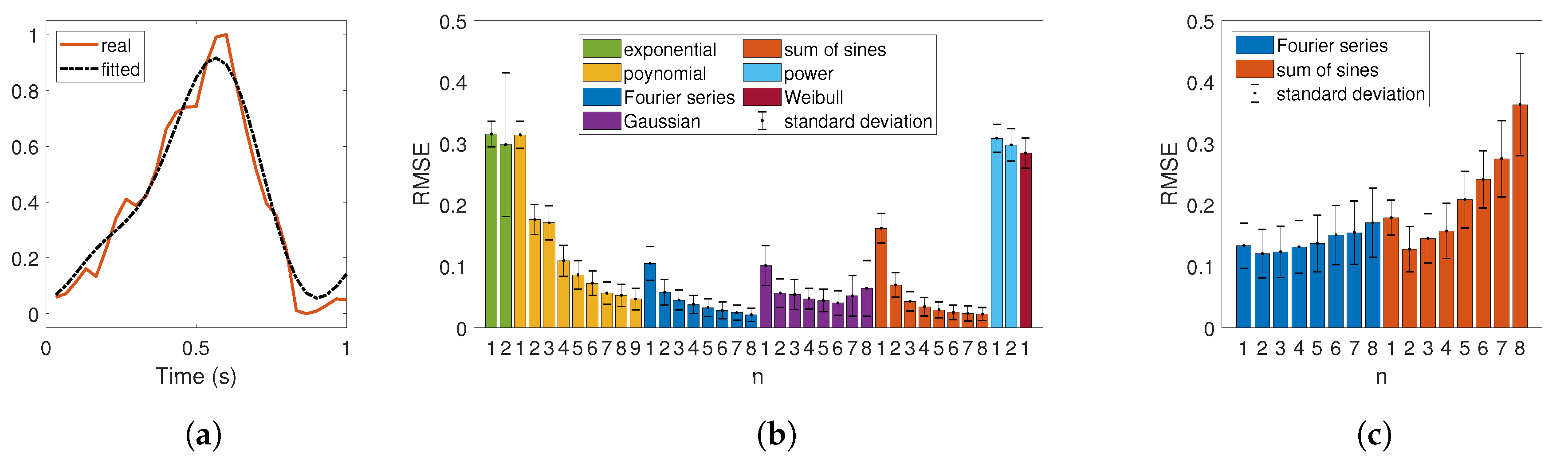
An RMSE value by pulse wave and by methods (here, a method refers to a model with a given n value, such as the polynomial model with , for example) was computed. Statistics (mean and standard deviation) are presented in Figure 4b. They show that the Fourier series and sum of sines models are the most relevant models. As expected, the RMSE decreases (goodness of fit increases) as we increase the number of terms (n) and therefore the number of coefficients. These models present a particular advantage: they fit periodic functions and can therefore be used to generate periodic functions.
Each method (e.g., Fourier series with ) currently includes 62 sets of and coefficients (one set of coefficients per PPG wave). We averaged the corresponding coefficients to get a unique model per method. As stated in the previous paragraph, only Fourier series and sum of sines models were considered. We computed once more the RMSE between the 2 × 8 average models and the 62 pulse waves extracted from the UBFC-RPPG dataset. Related results are presented in Figure 4c. Independently of the model, is the best choice (lowest RMSE). Overall, Fourier series for is the method that gives the lowest RMSE. Because the two models are pretty similar (see equations in Table 1), the error difference between them for is slight (average model RMSE for Fourier series: 0.12; average model RMSE for sum of sines model: 0.13). We can also observe that the RMSE increases as we increase n, probably because of overfitting that restricts generalization.
3.2.2. Signal Formation
Two-second pulse signals were generated by varying between 55 and 240 bpm (0.9 and 4 Hz) at regular intervals of 2.5 bpm for the Fourier series model:
corresponds to the scaling factor and to the mean value. We scaled the signal between 0 and 1. with Hz at intervals of Hz. s. The time sampling was set to 30 Hz. This value corresponds to the typical number of frames per second delivered by standard cameras. Thus, y corresponds to a vector that integrates 60 (2 s × 30 Hz) scalars. Values of and coefficients (Equation (2)) are presented in Table 2. The phase of the produced signal is randomly shifted using a uniform distribution.
3.2.3. Addition of Trends
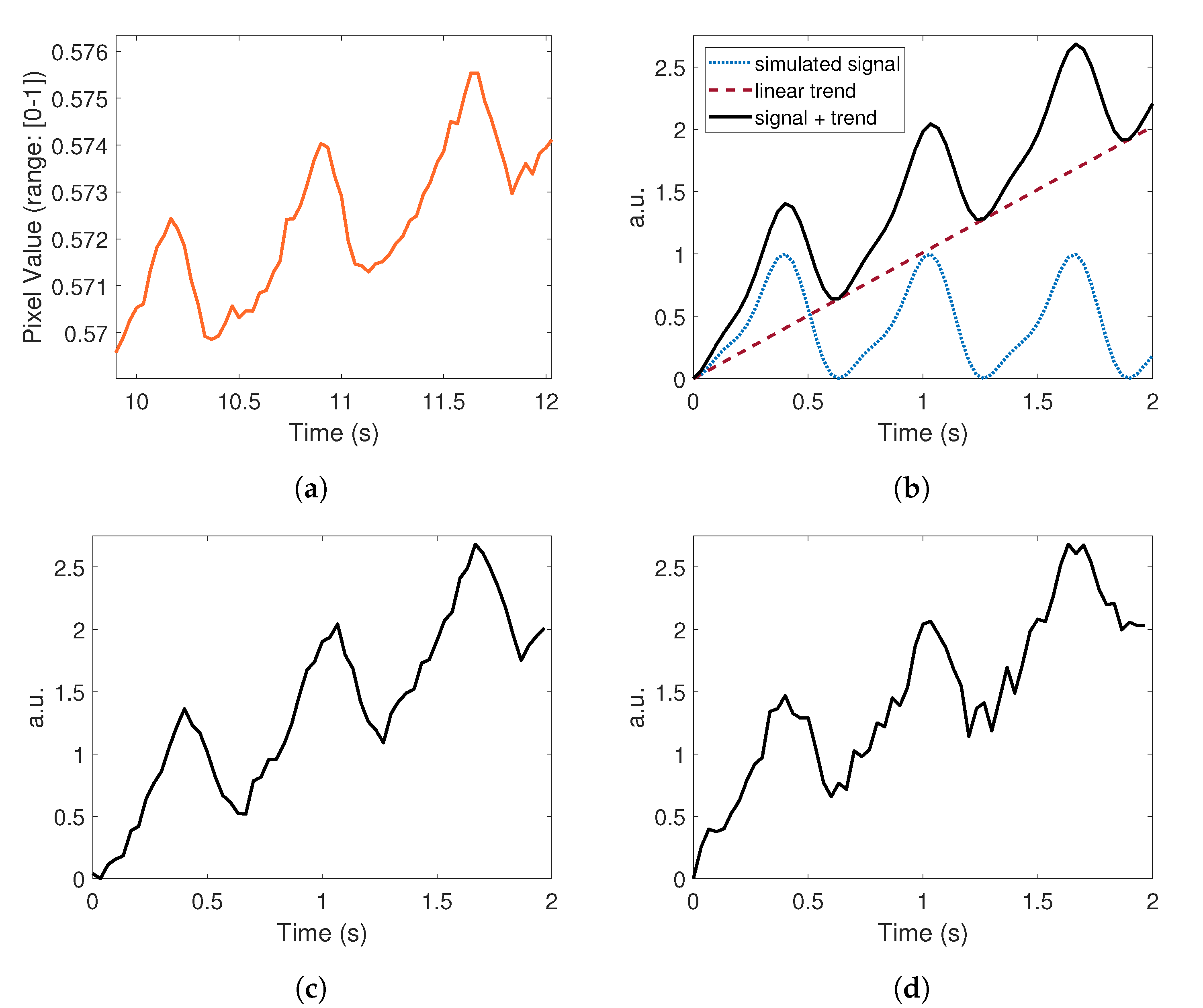
Linear, quadratic, or cubic tendency was added to the synthesized signal in order to reproduce fluctuations that naturally appear in real PPG signals. Here, (Equation (2)) corresponds to a linear vector instead of a scalar value. The slope (curve parameters) was randomly selected with a uniform distribution. The results of this procedure are illustrated in Figure 5 for the case of a linear tendency. Figure 5a shows an excerpt of a raw PPG signal (taken from subject #1, UBFC-RPPG dataset). Figure 5b depicts a simulated signal (dotted blue line) with its associated trend (dashed crimson line). The resulting signal is presented in a solid black line.
3.2.4. From 1D (Signal) to 3D (Video)
We transformed the unidimensional pulse signal y into a video stream using vector repetition (Figure 2d). At this stage, all the pixels in a frame share a unique value. This value gradually rises and falls as time progresses. The amplitude ( in Equation (3)) was randomly selected with a uniform distribution. The video corresponds to a volume v whose shape is 25 × 25 × 60.
3.2.5. Addition of Noise
Random noise was independently added to each frame (Figure 2e). This step reproduces natural fluctuations due to camera noise that randomly appear on images. The noise ( in Equation (3)) was added to each pixel of a frame using a normal (Gaussian) distribution (mean: 0.5, standard deviation: 0.25). Performing a simple spatial averaging operation [39] on these small video patches produces synthetic PPG signals (see Figure 5c,d for typical examples) that are quite similar to realistic ones (Figure 5a).
3.3. 3D CNN for Automatic Pulse Rate Estimation
A 3D CNN classifier structure was developed for both the extraction and classification of unprocessed video streams. The CNN acts as a feature extractor. Its final activations feed two dense layers (multilayer perceptron) that are used to classify pulse rate. The neural network was implemented and trained in Python using TensorFlow and Keras frameworks. All of the predicted data and statistics were processed with Matlab.
3.3.1. Network Architecture
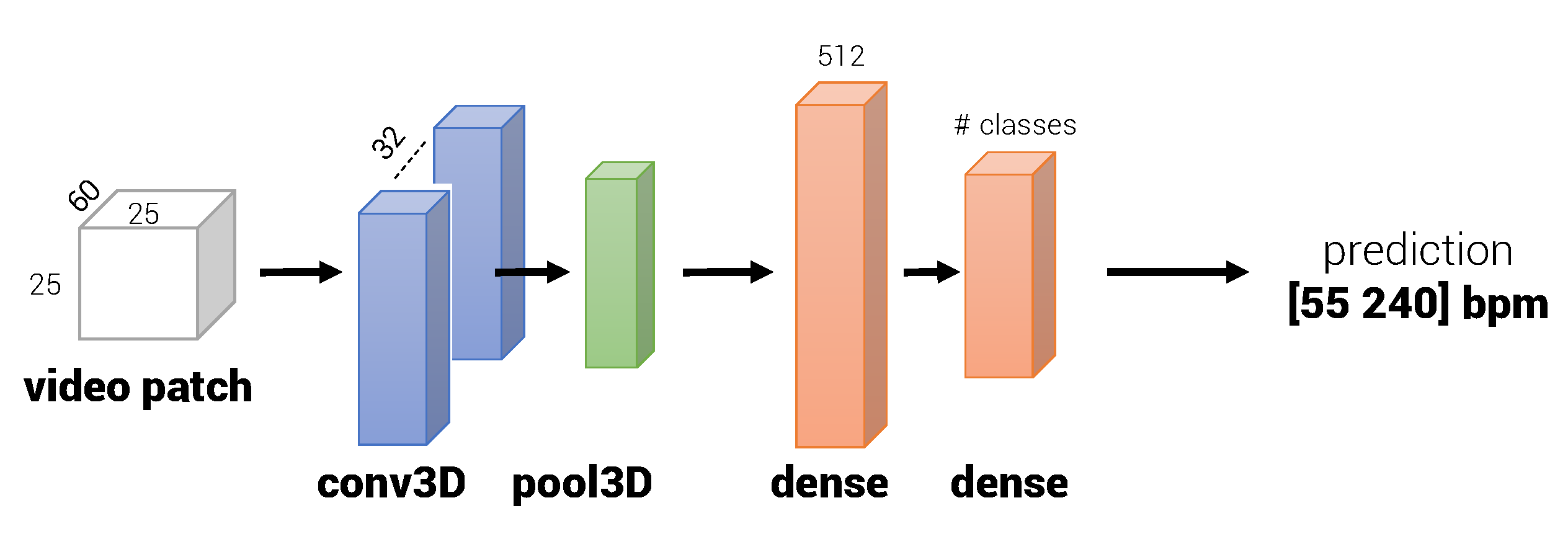
The complete architecture is presented in Figure 6. The convolution operations are performed by 32 3D filters (or kernels) of a 58 × 20 × 20 size. A 3D max pooling operation with a pool size of 2 × 2 × 2 follows the convolutional layer. Rectified linear unit (ReLU) is employed as an activation function. The CNN part of the network structure can be formalized as a set of three operations, namely, convolution (Equation (4)), pooling (Equation (5)), and non-linear activation (Equation (6)):
In Equation (4), corresponds to the convolutional layer inputs, i.e., a batch of synthetic video streams v (see Equation (3)). W is the weight matrix (learnable filters). ⊛ corresponds to the convolution operator. In Equation (5), denotes the 3D max pooling operation. An additional dropout operation (Equation (7)) has been introduced to regularize the CNN. Dropout regularization has proven to be very effective against overfitting [79]. r is a binary vector whose elements are randomly drawn. We randomly dropped out 20% of the total number of units in the convolutional layer.
The final activations of the CNN are then flattened and passed to a multilayer perceptron with a hidden layer that includes 512 neurons. The hidden layer is connected to the 76 output neurons: 75 for the pulse rates (55 to 240 bpm at regular intervals of 2.5 bpm) plus an extra "No PPG" class trained using synthetic videos of camera noise and illumination fluctuations. The activation functions for the first and second (output) dense layers are, respectively, ReLU and softmax functions. As for the convolutional layer, a dropout operation (fraction: 20%) is introduced to improve regularization.
3.3.2. Learning the Model
Backpropagation algorithm is currently the standard training method [79]. It is based on gradient descent to update the learnable parameters. Adam optimizer [80] was selected as an optimization function with an initial learning rate of . All weights were randomly initialized using the method proposed by Glorot and Bengio [81]. Biases were initialized to zero.
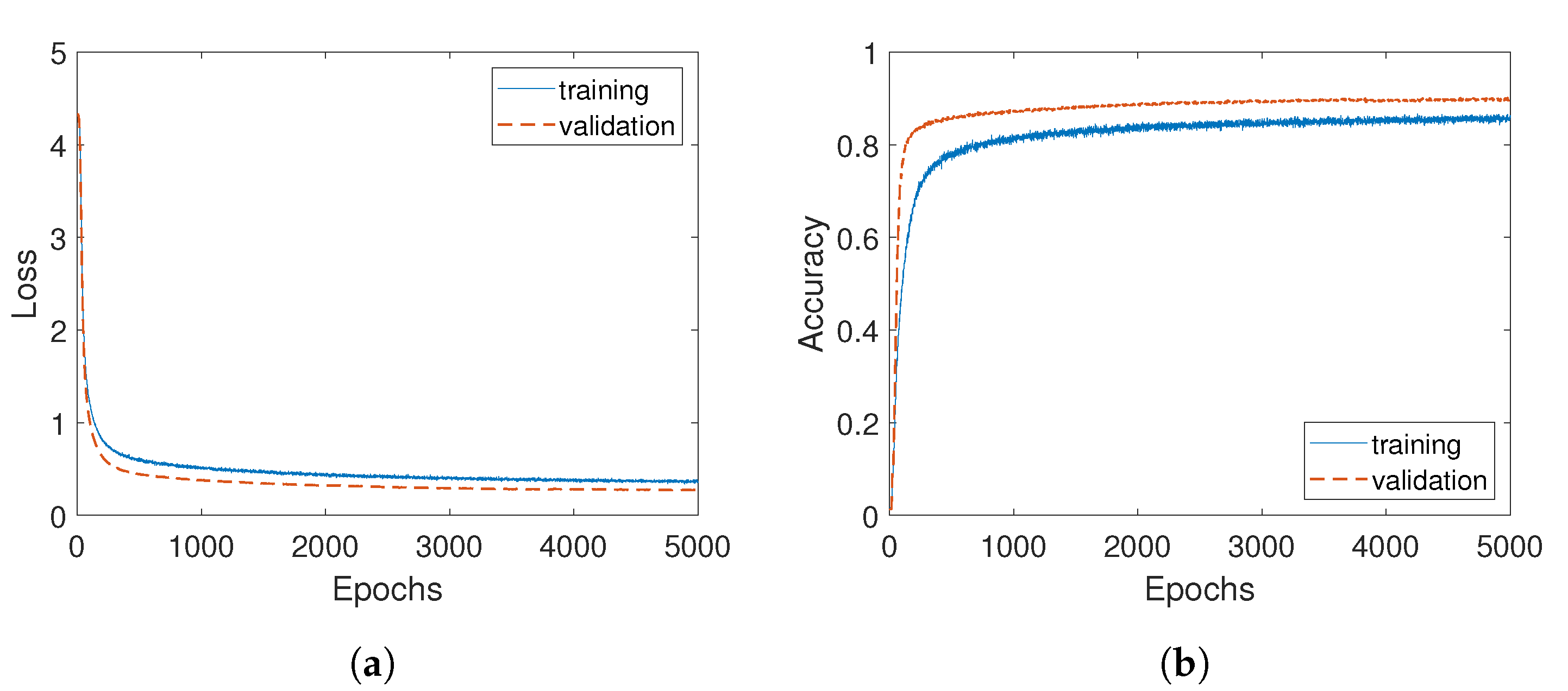
Each video was centered around zero by removing the mean value. Training was carried out by successively launching batches of 15,200 in size (200 video patches in each of 76 classes). Thus, each batch updated the weights of the networks according to an input tensor of a 15,200 × 25 × 25 × 60 size. New synthetic video patches were generated before passing a new batch to the network. We chose to pass a given batch of data to the network a single time (1 iteration). The number of epochs (which is the same as the number of batches because iteration = 1) was set to 5000.
We reserved a full batch of data for validation. We used this set to monitor the training process by stopping the procedure with an early-stopping criterion based on overfitting detection. We used categorical cross-entropy as a loss function. In practice, we observed that the training procedure converged well before the 5000th epoch, the decrease in validation loss becoming negligible (Figure 7a). Validation accuracy was greater than training accuracy, both being greater than 0.9 (Figure 7b). Dropout regularization presumably caused this particularity. These metrics are, of course, completely virtual since the model learned only synthetic data. We next present pulse rate estimations that were computed on real PPG videos using the 3D CNN model trained on synthetic data.
3.3.3. Pulse Rate Prediction
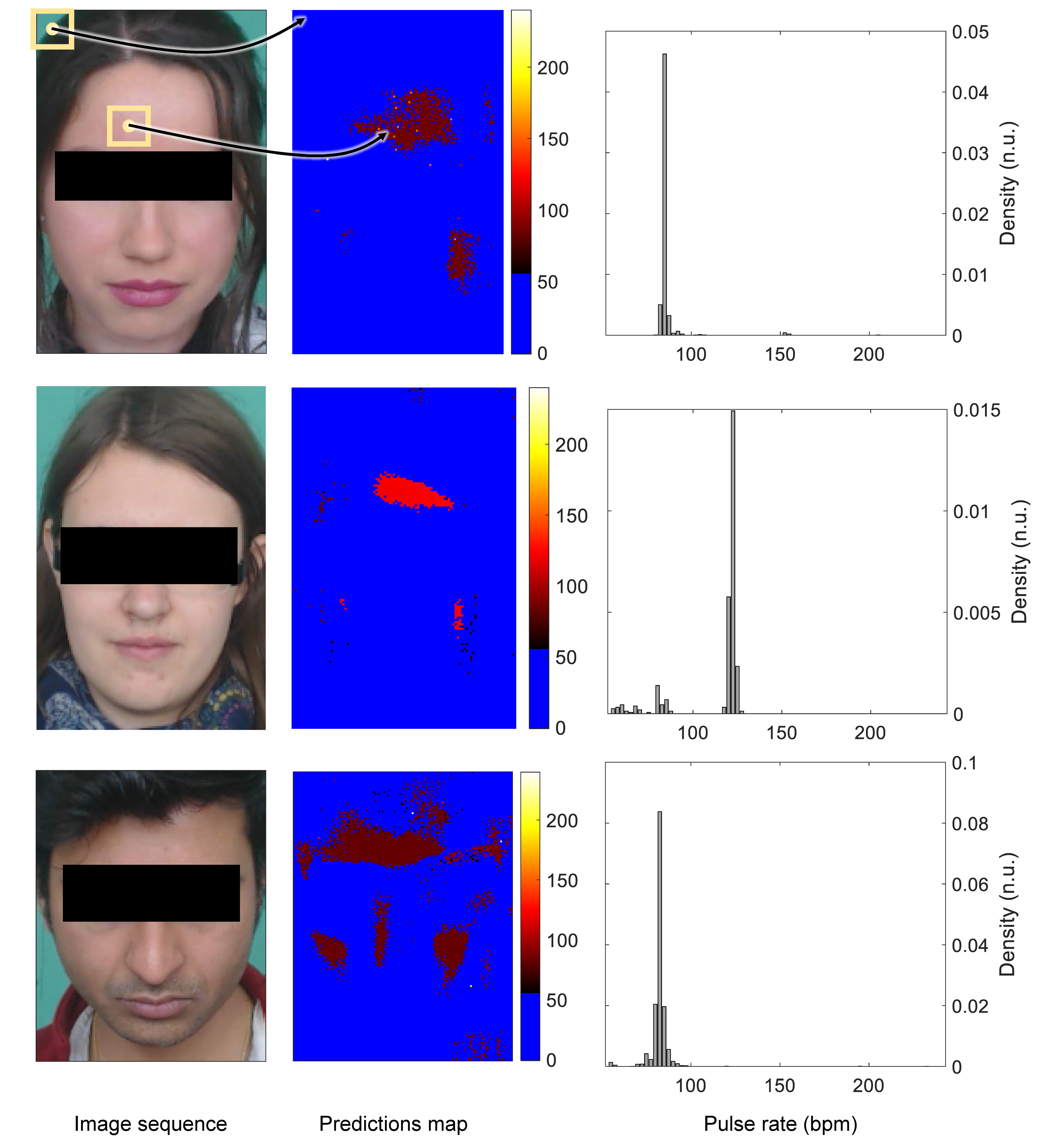
The learned model produces a prediction for a volume of 25 × 25 × 60 pixels. The synthetic data generator used to train the model does not incorporate a stage ensuring that the frames in the 25 × 25 patches contain pixels that are naturally arranged and ordered like in real video streams. We therefore chose to break the coherent structure of pixels before predicting the pulse rate by shuffling the pixel position. Note that only the green channel [39] was processed by the model.
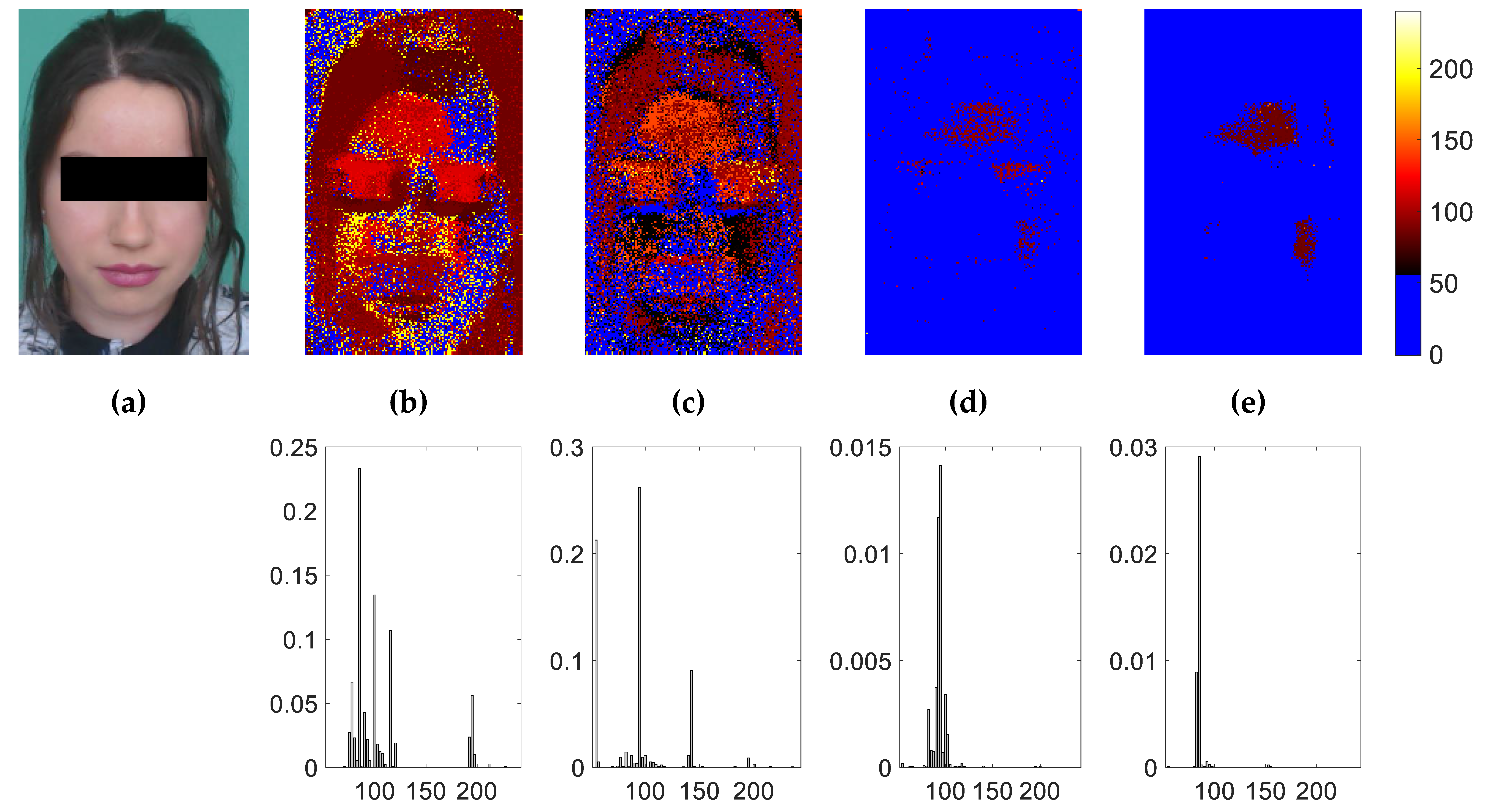
Maps of predictions were formed by computing a prediction for each group of pixels in the video stream. The procedure predicts and then shifts the input volume with a constant spatial step of 1 pixel (with overlapping). Typical prediction maps computed from the first 60 frames of subjects #1, #33, and #42 (UBFC-RPPG dataset) are presented in Figure 8. Blue pixels correspond to regions where no distinct PPG variations were identified (e.g., background and hair), while the other colors refer to properly predicted pulse rate values. It is important to emphasize that the network gives a score for each class (all pulse rate values plus a “No PPG” class) and that only the class that presents the highest score is saved and presented in these maps.
We can visually observe that the majority of pulse pixels are located in relevant regions like the cheeks and forehead. These areas contain significant PPG signal-to-noise ratios. The maps are somewhat similar to those presented in [82].
The right illustrations on Figure 8 present the histograms computed from the maps of predictions. They exhibit a dominant pulse rate (main peak) of 85, 122.5, and 82.5 bpm for subjects #1, #25, and #42, respectively. The corresponding ground-truth pulse rates for these examples are, respectively, 90, 122, and 81 bpm. The histograms have been normalized so that their total energy is equal to 1. Only the bins that correspond to pulse rates are presented. The final pulse rate was computed by aggregating all of the bins in the histogram of predictions using a weighted average operation:
corresponds to the pulse rate value outputted by the method, f to the frequency (55 to 240 bpm at regular intervals of 2.5 bpm), and to the amplitude (number of pixels) of a bin.
4. Results and Discussion
The UBFC-RPPG dataset [20] was selected to assess the performance of the neural network presented in Section 3. From the initial dataset, we manually removed image sequences in which the participant presented no distinct PPG signal (due particularly to wide head movements) or in case of corrupted ground-truth signals. In total, 1312 pulse rate values from 15 participants were extracted from the initial dataset.
The benchmark methods (presented hereafter) operate more efficiently with prior skin detection, robust face tracking, or when pixels of interest are segmented beforehand [46]. Therefore, and in order to provide fair comparisons, the forehead or the cheeks (when the forehead was covered with hair) were manually selected as regions of interest.
4.1. Evaluation Metrics and Methods
In this section, we detail the metrics and methods employed for evaluating the performance of the neural network. We selected the mean of pulse rate error (ME), standard deviation of pulse rate error (STDE), mean absolute error (MAE, see Equation (9)), and RMSE (Equation (10)), along with Bland–Altman plots to quantify the level of agreement between the estimated and ground-truth pulse rate values.
Here, the pulse rate estimated from the image sequence is denoted (Equation (8)), and the ground-truth pulse rate is denoted as . Pulse rate values estimated with the 3D CNN network were also compared with other state-of-the-art methods:
These four methods were implanted using iPhys, an open toolbox released by McDuff and Blackford [83]. The red, green, and blue signals were interpolated with a shape-preserving cubic function to 30 Hz before launching the methods. After computing their respective PPG signals, the four benchmark methods share a common procedure: We processed the signal with a 3rd order Butterworh filter with cutoff frequencies set to [0.667, 4] Hz, which correspond to [40, 240] bpm. The signal was then interpolated with a cubic spline function at a frequency of 256 Hz to refine peaks. Beat-to-beat pulse rate values were finally computed from the interbeat intervals.
4.2. Results Analysis
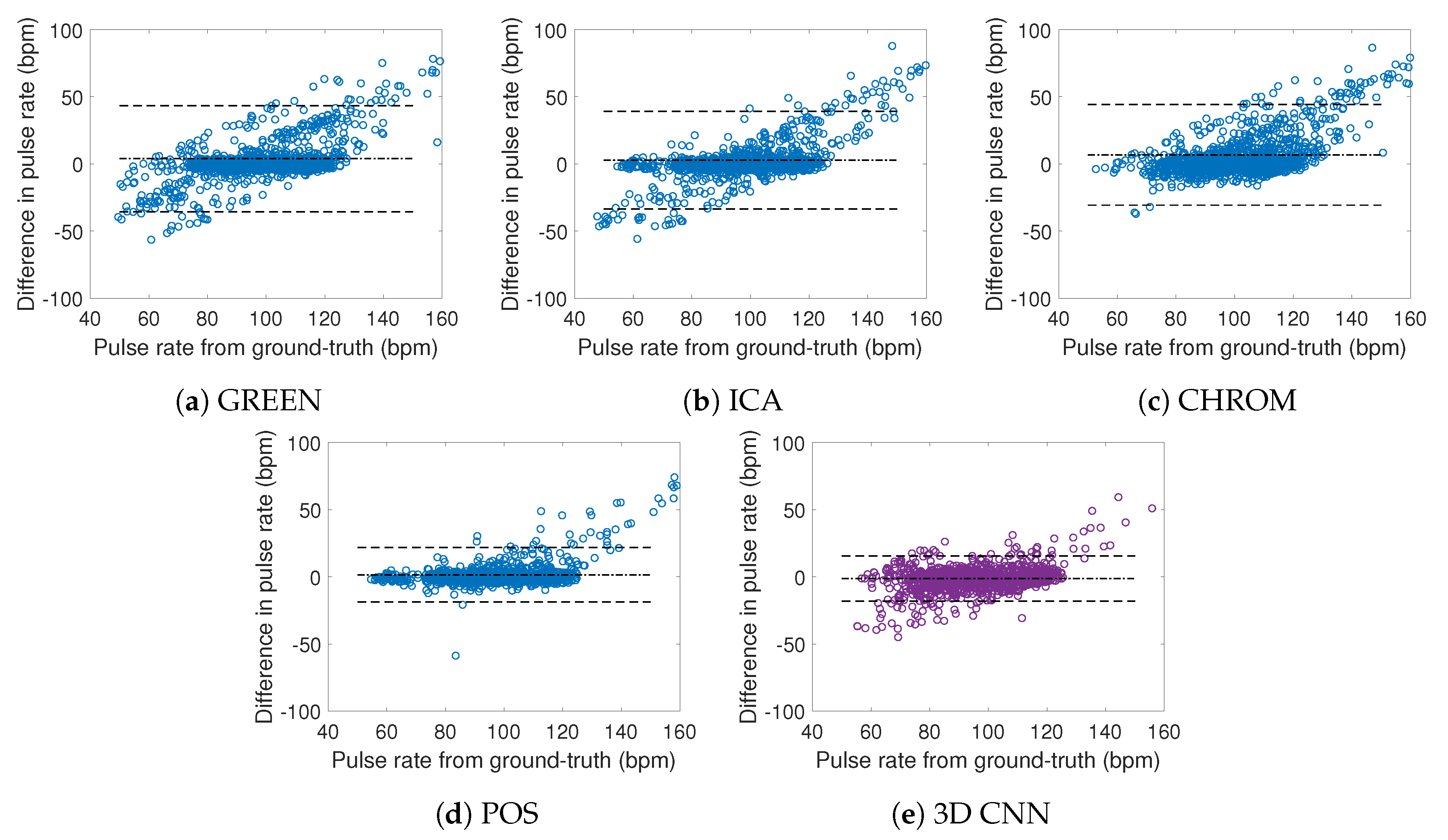
General results are summarized in Table 3, while a typical excerpt is presented in Figure 9. The Bland–Altman plots presented in Figure 10 represent the differences between estimates against ground-truth measurements. Means are represented by dash-dot lines and 95% limits of agreement (±1.96 SD) by dashed lines. Note that each ME value in Table 3 corresponds to each dash-dot line in the Bland–Altman representations.
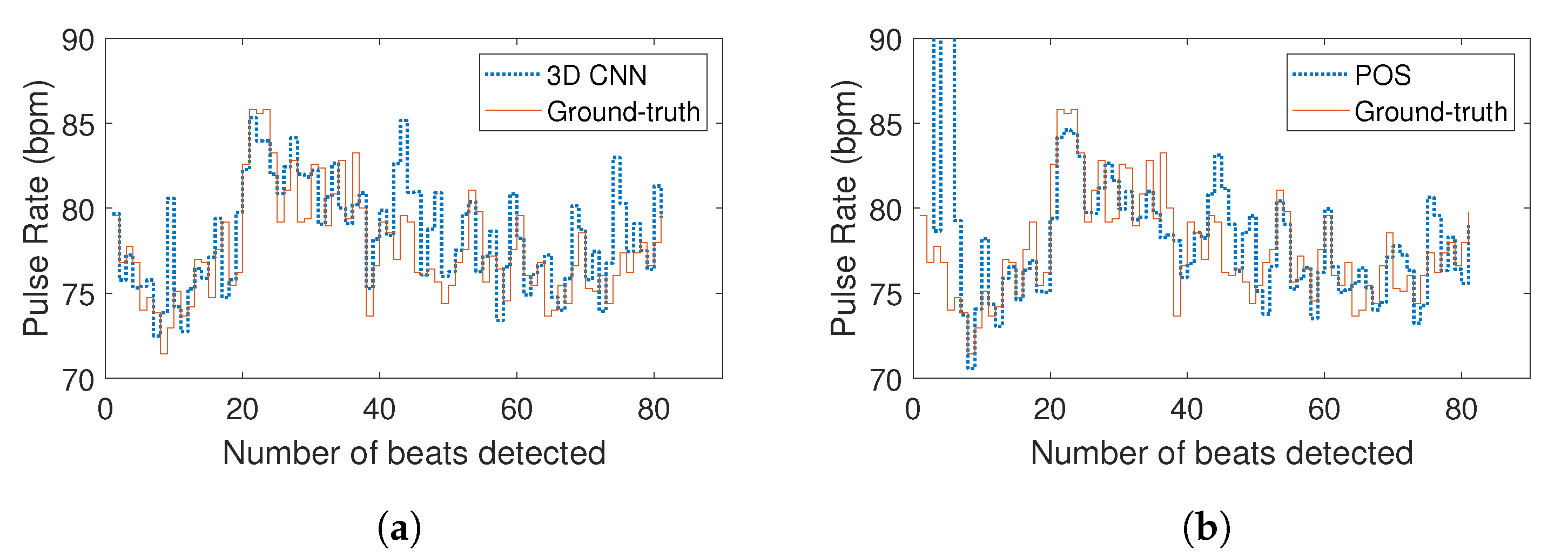
The results presented in Table 3 exhibit significant agreement between the estimated and ground-truth measurements: the RMSE computed from the pulse rate values assessed with the 3D CNN is lower than for the other methods. The MAE is, however, the lowest for POS, which is globally the most relevant benchmark method. Figure 9a,b presents the estimation for subject #31. Apart from the couple of erroneous beats at the beginning of the POS series, both methods performed well.
In addition, and concurrently with previous findings, GREEN, which is in fact the most straightforward method, produced noisy PPG signals and thus pulse rate series full of artifacts. GREEN presents the largest RMSE and standard deviation of pulse rate error. Surprisingly, metrics computed from CHROM estimations are very close to GREEN ones. This contrasts with the findings of Bobbia et al. [20], in which CHROM was even superior to POS. It is worth mentioning that the results cannot be directly compared because image processing techniques like skin detection and super-pixels were used in their work. These methods improved the signal-to-noise ratio and reduced noise and artifacts from PPG signals.
The Bland–Altman plots confirm the metrics presented in Table 3. The distribution is far wider for GREEN, ICA, and CHROM methods than for 3D CNN and POS. Visually, it can be observed that the distribution is more concentrated for POS (Figure 10d) than 3D CNN (Figure 10e). From this observation, we can conclude that POS estimations are globally more accurate, while the method we propose presents fewer irrelevant beats (which are characterized by outliers in the figures). Excluding these artifacts from pulse rate series with a dedicated filtering technique [50] would presumably ascertain this remark. This kind of procedure has not been included because the main objective consisted in assessing the relevance of direct beat-to-beat pulse rate values.
Training and prediction were executed on a computer equipped with an Intel Xeon CPU E5-1607 v4 and a GPU NVIDIA GeForce GTX 1080 Ti. Without any software or hardware optimization, estimating a pulse rate value from a 25 × 25 × 60 video patch takes 4 ms.
4.3. Improving the Network Architecture
The model achieved valuable results in regard to the shallow network architecture proposed in this work. Recent deep learning models adopted or built for the purpose of blood volume pulse [57] or pulse rate [61] measurement from videos exhibit significant results, in particular for image sequences that contain wide head movements. The shallow architecture proposed in this work may not compete with these deep models.
The main objective of this pilot study was to assess the limits and potential of 3D CNN in the context of PPG measurement from image sequences. We therefore envisage improving the network architecture in order to get more promising results. One of the main avenues consists in increasing the number of hidden (i.e., 3D CNN) layers and integrating optimized distributed gradient boosting (XGBoost). XGBoost is a widely used method that achieves state-of-the-art results in many machine learning challenges [84].
An iterative, grid-based procedure should be developed to assess the impact of network architecture (e.g., number of layers, number of filters per convolutional layer, and number of neurons per dense layer) and hyper-parameters on performance. This procedure could provide an objective and automatic way of selecting the network architecture that achieves the highest performance.
Only video patches of a 25 × 25 × 60 size were analyzed by the neural network. Varying these values or adopting a spatiotemporal multiscale approach [66] should be investigated in future work. In addition, the learned pulse rate values were sampled with a constant 2.5 bpm step. Rising the sensitivity of the model by reducing this interval could be particularly interesting.
4.4. Maps Convergence during Training
Figure 11 presents some prediction maps associated with temporary models that were generated throughout training. The maps were computed from the first 60 frames of subject #1. The associated histograms are presented in bottom row.
We can visually observe that the pixels labeled with pulse rates converged into relevant areas (i.e., forehead and cheeks) as the neural network learned, while pixels that contain no PPG information (blue pixels, e.g., from the background) were properly identified. In addition, the maps at the beginning of the learning procedure (Figure 11b,c contain disparate pulse rate values, resulting in high entropy histograms. After several epochs (Figure 11d,e), the entropy is lowered because the maps contain one or two prevailing pulse rate values. The histogram entropy, computed using Shannon’s formula, can here be assimilated to a confidence index: the lesser the entropy, the better the prediction.
4.5. Non-Stationary Signals and Motion
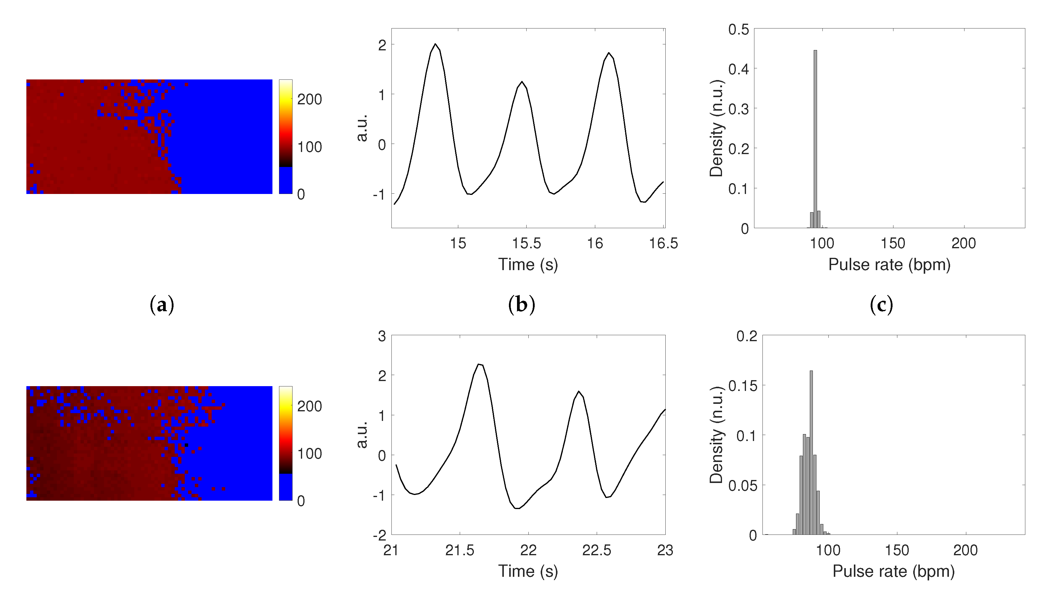
The UBFC-RPPG dataset contains videos during which the participants played a time-sensitive mathematical game that supposedly raised their pulse rate. High pulse rate values can effectively be observed on the Bland–Altman plots (Figure 10). In addition to natural motion (head movements), the game tends to drastically change the PPG signal frequency over time. These signals are thus predominantly non-stationary. This has not been considered in the method we propose in this study, the synthetic generator (Section 3.2) producing only stationary signals.
Non-stationary PPG signals have an impact on the histogram distribution computed from the prediction maps. Figure 12 presents a typical example: the more a video patch contains a non-stationary PPG signal (Figure 12b, bottom row), the more bins are present in the histogram of predictions (Figure 12c, bottom row), which thus increases entropy and reduces the pulse rate prediction accuracy.
Strong and wide movements were not considered in this work: except for the trends (Section 3.2.3), the network has not been trained with data that includes motion artifacts. In addition, natural variations of the trend observed in an image sequence may not follow a linear, quadratic, or cubic order. We believe that there is room for improvement and plan to investigate further in this direction. If a deeper architecture is adopted, transfer learning and/or fine-tuning approaches could be viable options for increasing performance and, presumably, handling motion [61].
4.6. Other Future Developments
Quality of the predicted maps: We plan to cross each map of predictions with a skin mask in order to assess the relevance of the detection. Metrics like precision, which is expected to be high, and recall could be used for this purpose.
Only the class (pulse rate value) that presents the highest score was saved and presented in the prediction maps. The network, however, attributes to each class a score, and we believe that this information could be exploited to improve prediction performance.
Currently, the method accepts as input only a single channel. We therefore did not consider color as we processed only the green channel. We plan to enhance the network and compare the impact of color on performance, especially in terms of pulse rate accuracy and artifact removal.
5. Conclusions
The main objective of the pilot study we present in this article consisted in assessing the potential and limits of 3D convolutional neural networks dedicated to the estimation of pulse rate from video streams. The results show that this solution is promising in this particular context, despite the shallow network architecture. We envisage comparing the proposed method with other deep learning architectures developed to measure blood volume pulse or pulse rate from facial videos.
There is room for improvement here: adding more convolutional layers to the network is the principal avenue that must be investigated next. Of course, a limited number of 3D CNN layers can be added because of the computational burden that compromises training. The impact of other types of layers, like recurrent neural networks, should also be investigated. A multiresolution approach could be of interest in order to overcome varying image resolution and distance. Both spatial and temporal resolutions can be considered with this kind of approach.
Author Contributions
Conceptualization, F.B. and A.P.; methodology, F.B.; software, F.B.; validation, F.B., C.M., and A.P.; investigation, F.B.; resources, A.P.; writing–original draft preparation, F.B.; supervision, F.B., C.M., and A.P.
Funding
This research received no external funding.
Conflicts of Interest
The authors declare no conflict of interest.
References
- Balakrishnan, G.; Durand, F.; Guttag, J. Detecting pulse from head motions in video. In Proceedings of the 2013 IEEE Conference on Computer Vision and Pattern Recognition (CVPR), Portland, OR, USA, 23–28 June 2013; pp. 3430–3437. [Google Scholar]
- Hassan, M.; Malik, A.; Fofi, D.; Saad, N.; Karasfi, B.; Ali, Y.; Meriaudeau, F. Heart rate estimation using facial video: A review. Biomed. Signal Process. Control 2017, 38, 346–360. [Google Scholar] [CrossRef]
- Haque, M.A.; Irani, R.; Nasrollahi, K.; Moeslund, T.B. Heartbeat rate measurement from facial video. IEEE Intell. Syst. 2016, 31, 40–48. [Google Scholar] [CrossRef]
- Wu, H.Y.; Rubinstein, M.; Shih, E.; Guttag, J.; Durand, F.; Freeman, W. Eulerian Video Magnification for Revealing Subtle Changes in the World. ACM Trans. Graph. 2012, 31, 65:1–65:8. [Google Scholar] [CrossRef]
- Ordóñez, C.; Cabo, C.; Menéndez, A.; Bello, A. Detection of human vital signs in hazardous environments by means of video magnification. PLoS ONE 2018, 13, e0195290. [Google Scholar] [CrossRef]
- Zaunseder, S.; Trumpp, A.; Wedekind, D.; Malberg, H. Cardiovascular assessment by imaging photoplethysmography—A review. Biomed. Eng./Biomedizinische Technik 2018, 63, 617–634. [Google Scholar] [CrossRef] [PubMed]
- Allen, J. Photoplethysmography and its application in clinical physiological measurement. Physiol. Meas. 2007, 28, R1–R39. [Google Scholar] [CrossRef] [PubMed] [Green Version]
- Kamshilin, A.A.; Nippolainen, E.; Sidorov, I.S.; Vasilev, P.V.; Erofeev, N.P.; Podolian, N.P.; Romashko, R.V. A new look at the essence of the imaging photoplethysmography. Sci. Rep. 2015, 5, 10494. [Google Scholar] [CrossRef]
- Shao, D.; Liu, C.; Tsow, F.; Yang, Y.; Du, Z.; Iriya, R.; Yu, H.; Tao, N. Noncontact monitoring of blood oxygen saturation using camera and dual-wavelength imaging system. IEEE Trans. Biomed. Eng. 2016, 63, 1091–1098. [Google Scholar] [CrossRef]
- Van Gastel, M.; Stuijk, S.; De Haan, G. New principle for measuring arterial blood oxygenation, enabling motion-robust remote monitoring. Sci. Rep. 2016, 6, 38609. [Google Scholar] [CrossRef] [Green Version]
- Hassan, M.; Malik, A.; Fofi, D.; Saad, N.; Meriaudeau, F. Novel health monitoring method an using RGB camera. Biomed. Opt. Express 2017, 8, 4838–4854. [Google Scholar] [CrossRef]
- Van Gastel, M.; Stuijk, S.; de Haan, G. Robust respiration detection from remote photoplethysmography. Biomed. Opt. Express 2016, 7, 4941–4957. [Google Scholar] [CrossRef] [Green Version]
- Al-Naji, A.; Chahl, J. Simultaneous Tracking of Cardiorespiratory Signals for Multiple Persons Using a Machine Vision System With Noise Artifact Removal. IEEE J. Transl. Eng. Health Med. 2017, 5, 1–10. [Google Scholar] [CrossRef]
- Sugita, N.; Yoshizawa, M.; Abe, M.; Tanaka, A.; Homma, N.; Yambe, T. Contactless Technique for Measuring Blood-Pressure Variability from One Region in Video Plethysmography. J. Med. Biol. Eng. 2019, 39, 76–85. [Google Scholar] [CrossRef]
- Zhang, G.; Shan, C.; Kirenko, I.; Long, X.; Aarts, R.M. Hybrid optical unobtrusive blood pressure measurements. Sensors 2017, 17, 1541. [Google Scholar] [CrossRef]
- Bousefsaf, F.; Maaoui, C.; Pruski, A. Peripheral vasomotor activity assessment using a continuous wavelet analysis on webcam photoplethysmographic signals. Bio-Med. Mater. Eng. 2016, 27, 527–538. [Google Scholar] [CrossRef]
- Trumpp, A.; Schell, J.; Malberg, H.; Zaunseder, S. Vasomotor assessment by camera-based photoplethysmography. Curr. Dir. Biomed. Eng. 2016, 2, 199–202. [Google Scholar] [CrossRef]
- Kamshilin, A.A.; Zaytsev, V.V.; Mamontov, O.V. Novel contactless approach for assessment of venous occlusion plethysmography by video recordings at the green illumination. Sci. Rep. 2017, 7, 464. [Google Scholar] [CrossRef]
- Wang, W.; Stuijk, S.; de Haan, G. Living-Skin Classification via Remote-PPG. IEEE Trans. Biomed. Eng. 2017, 64, 2781–2792. [Google Scholar] [PubMed]
- Bobbia, S.; Macwan, R.; Benezeth, Y.; Mansouri, A.; Dubois, J. Unsupervised skin tissue segmentation for remote photoplethysmography. Pattern Recognit. Lett. 2019, 124, 82–90. [Google Scholar] [CrossRef]
- Al-Naji, A.; Gibson, K.; Lee, S.H.; Chahl, J. Monitoring of Cardiorespiratory Signal: Principles of Remote Measurements and Review of Methods. IEEE Access 2017, 5, 15776–15790. [Google Scholar] [CrossRef]
- Hurter, C.; McDuff, D. Cardiolens: Remote Physiological Monitoring in a Mixed Reality Environment; ACM SIGGRAPH 2017 Emerging Technologies; ACM: New York, NY, USA, 2017; p. 6. [Google Scholar]
- Villarroel, M.; Guazzi, A.; Jorge, J.; Davis, S.; Watkinson, P.; Green, G.; Shenvi, A.; McCormick, K.; Tarassenko, L. Continuous non-contact vital sign monitoring in neonatal intensive care unit. Healthc. Technol. Lett. 2014, 1, 87–91. [Google Scholar] [CrossRef] [PubMed]
- Zhang, Q.; Zhou, Y.; Song, S.; Liang, G.; Ni, H. Heart Rate Extraction Based on Near-Infrared Camera: Towards Driver State Monitoring. IEEE Access 2018, 6, 33076–33087. [Google Scholar] [CrossRef]
- Liu, S.; Yuen, P.C.; Zhang, S.; Zhao, G. 3D mask face anti-spoofing with remote Photoplethysmography. In Proceedings of the European Conference on Computer Vision, Amsterdam, The Netherlands, 8–16 October 2016; Springer: Berlin/Heidelberg, Germany, 2016; pp. 85–100. [Google Scholar]
- LeCun, Y.; Bengio, Y.; Hinton, G. Deep learning. Nature 2015, 521, 436. [Google Scholar] [CrossRef]
- Huang, P.H.; Chang, C.C.; Huang, C.Y.; Hsiao, T.C. Can Very High Frequency Instantaneous Pulse Rate Variability Serve as an Obvious Indicator of Peripheral Circulation? J. Commun. Comput. 2017, 14, 65–72. [Google Scholar]
- Long, J.; Shelhamer, E.; Darrell, T. Fully convolutional networks for semantic segmentation. In Proceedings of the IEEE Conference on Computer Vision and Pattern Recognition, Boston, MA, USA, 7–12 June 2015; pp. 3431–3440. [Google Scholar]
- Karpathy, A.; Toderici, G.; Shetty, S.; Leung, T.; Sukthankar, R.; Fei-Fei, L. Large-scale video classification with convolutional neural networks. In Proceedings of the IEEE Conference on Computer Vision and Pattern Recognition, Columbus, OH, USA, 23–28 June 2014; pp. 1725–1732. [Google Scholar]
- Guo, Y.; Liu, Y.; Oerlemans, A.; Lao, S.; Wu, S.; Lew, M.S. Deep learning for visual understanding: A review. Neurocomputing 2016, 187, 27–48. [Google Scholar] [CrossRef]
- Young, T.; Hazarika, D.; Poria, S.; Cambria, E. Recent trends in deep learning based natural language processing. IEEE Comput. Intell. Mag. 2018, 13, 55–75. [Google Scholar] [CrossRef]
- Graves, A.; Jaitly, N. Towards end-to-end speech recognition with recurrent neural networks. In Proceedings of the International Conference on Machine Learning, Beijing, China, 21–26 June 2014; pp. 1764–1772. [Google Scholar]
- Abdel-Hamid, O.; Mohamed, A.r.; Jiang, H.; Deng, L.; Penn, G.; Yu, D. Convolutional neural networks for speech recognition. IEEE/ACM Trans. Audio Speech Lang. Process. 2014, 22, 1533–1545. [Google Scholar] [CrossRef]
- Shen, D.; Wu, G.; Suk, H.I. Deep learning in medical image analysis. Annu. Rev. Biomed. Eng. 2017, 19, 221–248. [Google Scholar] [CrossRef]
- Miotto, R.; Wang, F.; Wang, S.; Jiang, X.; Dudley, J.T. Deep learning for healthcare: Review, opportunities and challenges. Briefings Bioinform. 2017, 19, 1236–1246. [Google Scholar] [CrossRef]
- Kranjec, J.; Beguš, S.; Geršak, G.; Drnovšek, J. Non-contact heart rate and heart rate variability measurements: A review. Biomed. Signal Process. Control 2014, 13, 102–112. [Google Scholar] [CrossRef]
- McDuff, D.J.; Estepp, J.R.; Piasecki, A.M.; Blackford, E.B. A survey of remote optical photoplethysmographic imaging methods. Engineering in Medicine and Biology Society (EMBC). In Proceedings of the 2015 37th Annual International Conference of the IEEE, Milano, Italy, 25–29 August 2015; pp. 6398–6404. [Google Scholar]
- Takano, C.; Ohta, Y. Heart rate measurement based on a time-lapse image. Med Eng. Phys. 2007, 29, 853–857. [Google Scholar] [CrossRef] [PubMed]
- Verkruysse, W.; Svaasand, L.O.; Nelson, J.S. Remote plethysmographic imaging using ambient light. Opt. Express 2008, 16, 21434–21445. [Google Scholar] [CrossRef] [PubMed] [Green Version]
- Kamshilin, A.A.; Margaryants, N.B. Origin of Photoplethysmographic Waveform at Green Light. Phys. Procedia 2017, 86, 72–80. [Google Scholar] [CrossRef]
- van Gastel, M.; Stuijk, S.; de Haan, G. Motion robust remote-PPG in infrared. IEEE Trans. Biomed. Eng. 2015, 62, 1425–1433. [Google Scholar] [CrossRef] [PubMed]
- McDuff, D.; Gontarek, S.; Picard, R.W. Improvements in remote cardiopulmonary measurement using a five band digital camera. IEEE Trans. Biomed. Eng. 2014, 61, 2593–2601. [Google Scholar] [CrossRef] [PubMed]
- McDuff, D.J.; Blackford, E.B.; Estepp, J.R. The Impact of Video Compression on Remote Cardiac Pulse Measurement Using Imaging Photoplethysmography. In Proceedings of the 2017 12th IEEE International Conference on Automatic Face & Gesture Recognition (FG 2017), Washington, DC, USA, 30 May–3 June 2017; pp. 63–70. [Google Scholar]
- Poh, M.Z.; McDuff, D.J.; Picard, R.W. Non-contact, automated cardiac pulse measurements using video imaging and blind source separation. Opt. Express 2010, 18, 10762–10774. [Google Scholar] [CrossRef]
- Bousefsaf, F.; Maaoui, C.; Pruski, A. Continuous wavelet filtering on webcam photoplethysmographic signals to remotely assess the instantaneous heart rate. Biomed. Signal Process. Control 2013, 8, 568–574. [Google Scholar] [CrossRef]
- Bousefsaf, F.; Maaoui, C.; Pruski, A. Automatic Selection of Webcam Photoplethysmographic Pixels Based on Lightness Criteria. J. Med Biol. Eng. 2017, 37, 374–385. [Google Scholar] [CrossRef]
- Stricker, R.; Müller, S.; Gross, H.M. Non-contact video-based pulse rate measurement on a mobile service robot. In Proceedings of the 2014 RO-MAN: The 23rd IEEE International Symposium on Robot and Human Interactive Communication, Edinburgh, UK, 25–29 August 2014; pp. 1056–1062. [Google Scholar]
- Po, L.M.; Feng, L.; Li, Y.; Xu, X.; Cheung, T.C.H.; Cheung, K.W. Block-based adaptive ROI for remote photoplethysmography. Multimedia Tools Appl. 2018, 77, 6503–6529. [Google Scholar] [CrossRef]
- Wang, W.; den Brinker, A.C.; Stuijk, S.; de Haan, G. Algorithmic Principles of Remote PPG. IEEE Trans. Biomed. Eng. 2017, 64, 1479–1491. [Google Scholar] [CrossRef]
- Poh, M.Z.; McDuff, D.J.; Picard, R.W. Advancements in noncontact, multiparameter physiological measurements using a webcam. IEEE Trans. Biomed. Eng. 2011, 58, 7–11. [Google Scholar] [CrossRef] [PubMed]
- Bousefsaf, F.; Maaoui, C.; Pruski, A. Remote detection of mental workload changes using cardiac parameters assessed with a low-cost webcam. Comput. Biol. Med. 2014, 53, 154–163. [Google Scholar] [CrossRef] [PubMed]
- McDuff, D.; Gontarek, S.; Picard, R.W. Remote detection of photoplethysmographic systolic and diastolic peaks using a digital camera. IEEE Trans. Biomed. Eng. 2014, 61, 2948–2954. [Google Scholar] [CrossRef] [PubMed]
- Monkaresi, H.; Calvo, R.A.; Yan, H. A machine learning approach to improve contactless heart rate monitoring using a webcam. IEEE J. Biomed. Health Inform. 2014, 18, 1153–1160. [Google Scholar] [CrossRef]
- Osman, A.; Turcot, J.; El Kaliouby, R. Supervised learning approach to remote heart rate estimation from facial videos. In Proceedings of the 2015 11th IEEE International Conference and Workshops on Automatic Face and Gesture Recognition (FG), Ljubljana, Slovenia, 4–8 May 2015; Volume 1, pp. 1–6. [Google Scholar]
- Hsu, Y.; Lin, Y.L.; Hsu, W. Learning-based heart rate detection from remote photoplethysmography features. In Proceedings of the 2014 IEEE International Conference on Acoustics, Speech and Signal Processing (ICASSP), Florence, Italy, 4–9 May 2014; pp. 4433–4437. [Google Scholar]
- Hsu, G.S.; Ambikapathi, A.; Chen, M.S. Deep learning with time-frequency representation for pulse estimation from facial videos. In Proceedings of the 2017 IEEE International Joint Conference on Biometrics (IJCB), Denver, CO, USA, 1–4 October 2017; pp. 383–389. [Google Scholar]
- Chen, W.; McDuff, D. DeepPhys: Video-Based Physiological Measurement Using Convolutional Attention Networks. arXiv 2018, arXiv:1805.07888. [Google Scholar]
- Chen, W.; McDuff, D. DeepMag: Source Specific Motion Magnification Using Gradient Ascent. arXiv 2018, arXiv:1808.03338. [Google Scholar]
- Chaichulee, S.; Villarroel, M.; Jorge, J.; Arteta, C.; Green, G.; McCormick, K.; Zisserman, A.; Tarassenko, L. Multi-task Convolutional Neural Network for Patient Detection and Skin Segmentation in Continuous Non-contact Vital Sign Monitoring. In Proceedings of the 2017 12th IEEE International Conference on Automatic Face & Gesture Recognition (FG 2017), Washington, DC, USA, 30 May–3 June 2017; pp. 266–272. [Google Scholar]
- Špetlík, R.; Franc, V.; Matas, J. Visual Heart Rate Estimation with Convolutional Neural Network. In Proceedings of the British Machine Vision Conference, Newcastle, UK, 3–6 September 2018. [Google Scholar]
- Niu, X.; Han, H.; Shan, S.; Chen, X. Synrhythm: Learning a deep heart rate estimator from general to specific. In Proceedings of the 2018 24th International Conference on Pattern Recognition (ICPR), Beijing, China, 20–24 August 2018; pp. 3580–3585. [Google Scholar]
- Jindal, V.; Birjandtalab, J.; Pouyan, M.B.; Nourani, M. An adaptive deep learning approach for PPG-based identification. In Proceedings of the 2016 IEEE 38th Annual International Conference of the Engineering in Medicine and Biology Society (EMBC), Orlando, FL, USA, 16–20 August 2016; pp. 6401–6404. [Google Scholar]
- Su, P.; Ding, X.R.; Zhang, Y.T.; Liu, J.; Miao, F.; Zhao, N. Long-term blood pressure prediction with deep recurrent neural networks. In Proceedings of the 2018 IEEE EMBS International Conference on Biomedical & Health Informatics (BHI), Las Vegas, NV, USA, 4–7 March 2018; pp. 323–328. [Google Scholar]
- Ji, S.; Xu, W.; Yang, M.; Yu, K. 3D convolutional neural networks for human action recognition. IEEE Trans. Pattern Anal. Mach. Intell. 2013, 35, 221–231. [Google Scholar] [CrossRef]
- Tran, D.; Bourdev, L.; Fergus, R.; Torresani, L.; Paluri, M. Learning spatiotemporal features with 3d convolutional networks. In Proceedings of the IEEE International Conference on Computer Vision, Santiago, Chile, 11–18 December 2015; pp. 4489–4497. [Google Scholar]
- Varol, G.; Laptev, I.; Schmid, C. Long-term temporal convolutions for action recognition. IEEE Trans. Pattern Anal. Mach. Intell. 2018, 40, 1510–1517. [Google Scholar] [CrossRef]
- Graham, D.; Langroudi, S.H.F.; Kanan, C.; Kudithipudi, D. Convolutional Drift Networks for Video Classification. In Proceedings of the 2017 IEEE International Conference on Rebooting Computing (ICRC), Washington, DC, USA, 8–9 November 2017; pp. 1–8. [Google Scholar]
- Dwibedi, D.; Sermanet, P.; Tompson, J.; Diba, A.; Fayyaz, M.; Sharma, V.; Hossein Karami, A.; Mahdi Arzani, M.; Yousefzadeh, R.; Van Gool, L.; et al. Temporal Reasoning in Videos using Convolutional Gated Recurrent Units. In Proceedings of the IEEE Conference on Computer Vision and Pattern Recognition Workshops, Salt Lake City, UT, USA, 18–22 June 2018; pp. 1111–1116. [Google Scholar]
- Lea, C.; Reiter, A.; Vidal, R.; Hager, G.D. Segmental spatiotemporal cnns for fine-grained action segmentation. In Proceedings of the European Conference on Computer Vision, Amsterdam, The Netherlands, 8–16 October 2016; Springer: Berlin/Heidelberg, Germany, 2016; pp. 36–52. [Google Scholar]
- Wang, L.; Xiong, Y.; Wang, Z.; Qiao, Y.; Lin, D.; Tang, X.; Van Gool, L. Temporal segment networks for action recognition in videos. IEEE Trans. Pattern Anal. Mach. Intell. 2018, 41, 2740–2755. [Google Scholar] [CrossRef]
- Donahue, J.; Anne Hendricks, L.; Guadarrama, S.; Rohrbach, M.; Venugopalan, S.; Saenko, K.; Darrell, T. Long-term recurrent convolutional networks for visual recognition and description. In Proceedings of the IEEE Conference on Computer Vision and Pattern Recognition, Boston, MA, USA, 7–12 June 2015; pp. 2625–2634. [Google Scholar]
- Goodfellow, I.; Bengio, Y.; Courville, A.; Bengio, Y. Deep Learning; MIT Press: Cambridge, UK, 2016; Volume 1. [Google Scholar]
- Soleymani, M.; Lichtenauer, J.; Pun, T.; Pantic, M. A multimodal database for affect recognition and implicit tagging. IEEE Trans. Affect. Comput. 2012, 3, 42–55. [Google Scholar] [CrossRef]
- Heusch, G.; Anjos, A.; Marcel, S. A Reproducible Study on Remote Heart Rate Measurement. arXiv 2017, arXiv:1709.00962. [Google Scholar]
- Tuccillo, D.; Decencière, E.; Velasco-Forero, S.; Huertas-Company, M. Deep learning for studies of galaxy morphology. Proc. Int. Astron. Union 2016, 12, 191–196. [Google Scholar] [CrossRef] [Green Version]
- George, D.; Huerta, E. Deep Learning for real-time gravitational wave detection and parameter estimation: Results with Advanced LIGO data. Phys. Lett. B 2018, 778, 64–70. [Google Scholar] [CrossRef]
- Quang, D.; Chen, Y.; Xie, X. DANN: A deep learning approach for annotating the pathogenicity of genetic variants. Bioinformatics 2014, 31, 761–763. [Google Scholar] [CrossRef]
- Plis, S.M.; Hjelm, D.R.; Salakhutdinov, R.; Allen, E.A.; Bockholt, H.J.; Long, J.D.; Johnson, H.J.; Paulsen, J.S.; Turner, J.A.; Calhoun, V.D. Deep learning for neuroimaging: A validation study. Front. Neurosci. 2014, 8, 229. [Google Scholar] [CrossRef]
- Gu, J.; Wang, Z.; Kuen, J.; Ma, L.; Shahroudy, A.; Shuai, B.; Liu, T.; Wang, X.; Wang, G.; Cai, J.; et al. Recent advances in convolutional neural networks. Pattern Recognit. 2018, 77, 354–377. [Google Scholar] [CrossRef] [Green Version]
- Kingma, D.P.; Ba, J. Adam: A method for stochastic optimization. arXiv 2014, arXiv:1412.6980. [Google Scholar]
- Glorot, X.; Bengio, Y. Understanding the difficulty of training deep feedforward neural networks. In Proceedings of the Thirteenth International Conference on Artificial Intelligence and Statistics, Sardinia, Italy, 13–15 May 2010; pp. 249–256. [Google Scholar]
- Liu, J.; Luo, H.; Zheng, P.P.; Wu, S.J.; Lee, K. Transdermal optical imaging revealed different spatiotemporal patterns of facial cardiovascular activities. Sci. Rep. 2018, 8, 10588. [Google Scholar] [CrossRef]
- McDuff, D.; Blackford, E. iPhys: An Open Non-Contact Imaging-Based Physiological Measurement Toolbox. arXiv 2019, arXiv:1901.04366. [Google Scholar]
- Chen, T.; Guestrin, C. Xgboost: A scalable tree boosting system. In Proceedings of the 22nd ACM Sigkdd International Conference on Knowledge Discovery and Data Mining, San Francisco, CA, USA, 13–17 August 2016; ACM: New York, NY, USA, 2016; pp. 785–794. [Google Scholar]
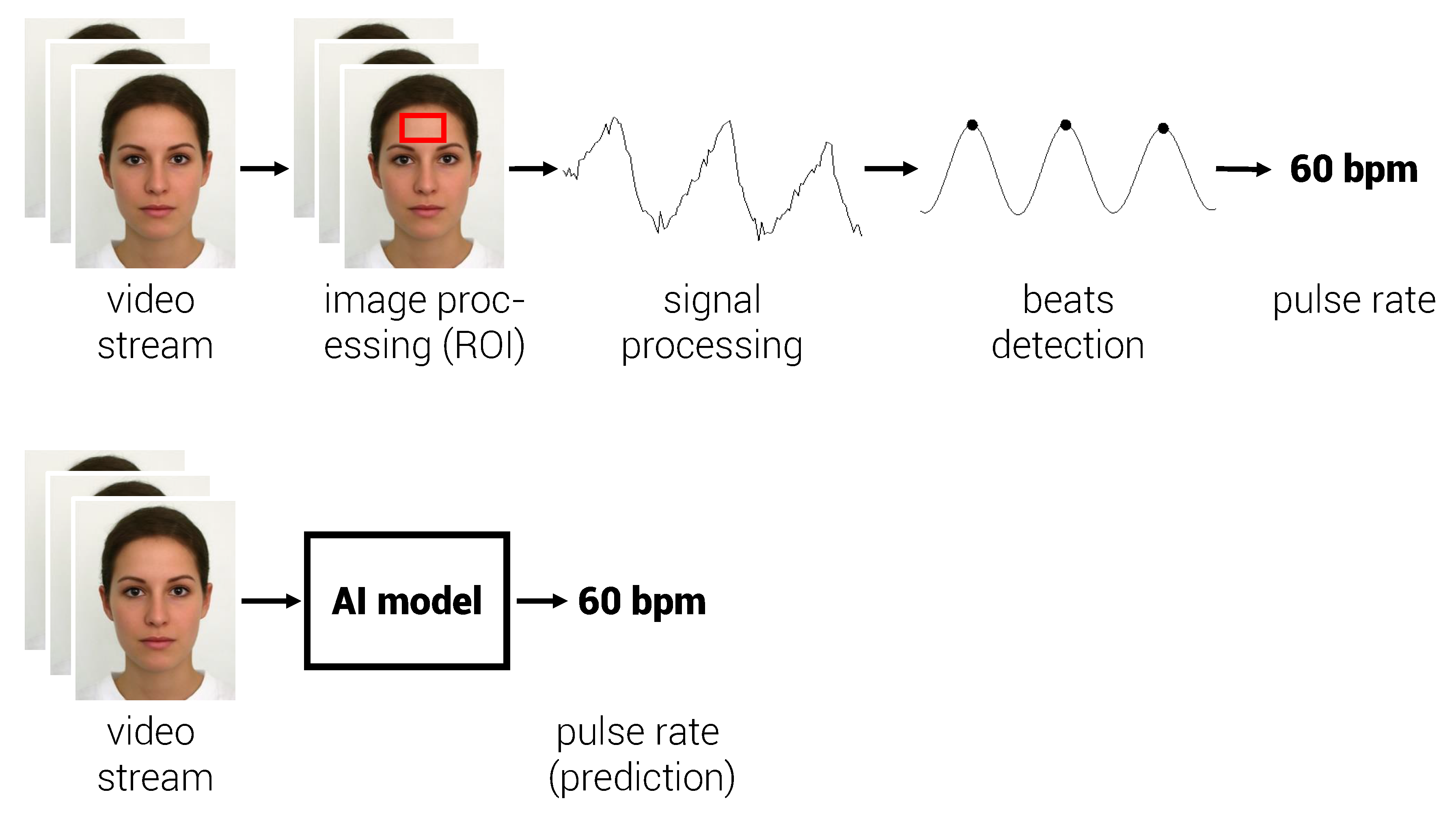
Figure 1.
(top) Conventional approach: image processing operations are applied to the video stream to detect pixels or regions of interest (ROIs). The signal is traditionally computed using a spatial averaging operation over the ROI before being processed with spectral or temporal filters. Finally, biomedical parameters like pulse rate are estimated from this signal. (bottom) The approach we propose consists in training an artificial intelligence model using only synthetic data. The input corresponds to a video stream (image sequence). The model predicts a pulse rate for each video patch (25 × 25 pixels over 60 frames) and thus produces a map of predictions instead of a single estimation.

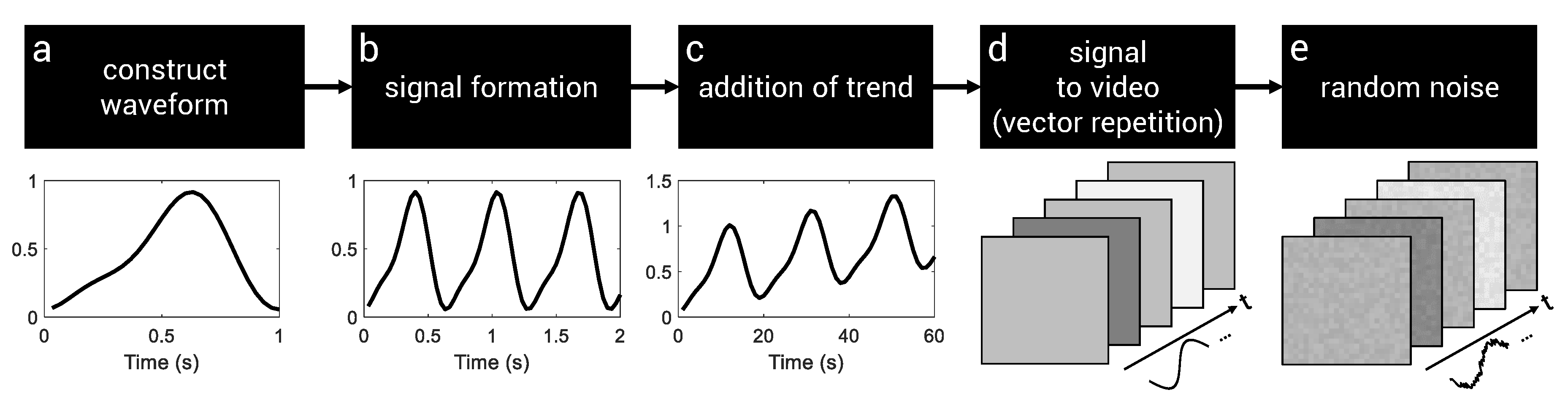
Figure 2.
Flowchart of the synthetic imaging photoplethysmography (iPPG) video generator approach. (a) A realistic pulse model approximated with Fourier series (sum of sine and cosine functions, see Figure 3 and Table 1) serves as the base waveform. (b) A two-second signal is produced from this waveform. (c) A linear, quadratic, or cubic tendency is added to the signal. (d) Videos are generated by repeating the signal for each pixel. (e) Random noise is independently added to each image of the video stream. This step reproduces natural fluctuations (due to camera noise) that randomly appear on images. Note that illustrations below blocks (d,e) have been magnified.

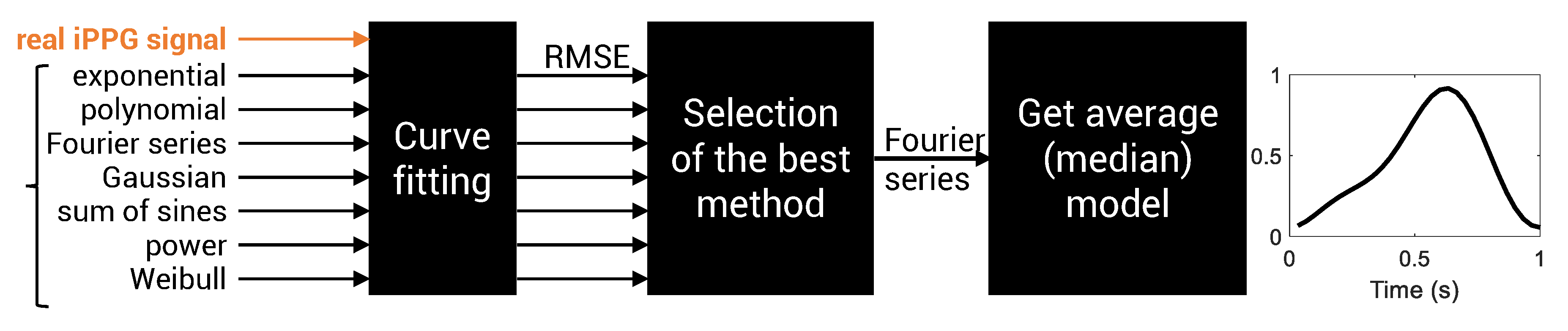
Figure 3.
Fitting real iPPG signals to determine the best pulse wave model. Different models are tested. Fourier series were chosen because they present the lowest root mean square error (RMSE, see Figure 4 for details). They also have the advantage of fitting periodic signals.
Figure 3.
Fitting real iPPG signals to determine the best pulse wave model. Different models are tested. Fourier series were chosen because they present the lowest root mean square error (RMSE, see Figure 4 for details). They also have the advantage of fitting periodic signals.

Figure 4.
Fitting results. (a) Typical excerpt of a camera pulse wave extracted from the UBFC-RPPG dataset. Solid orange line: raw photoplethysmography (PPG) pulse wave. Dotted black line: fitted signal. (b) Results of the curve-fitting procedure (periodic and non-periodic models were tested). The RMSE is computed for each of the 62 pulse waves and its corresponding fitted-to-data approximation. The statistics for each tested method (each histogram bin) indicates that Fourier series and sum of sines are the most relevant models. (c) Each method (e.g., Fourier series with ) contains 62 sets of and coefficients (one set of coefficients per PPG wave). We thus choose to respectively average the coefficients to produce a unique set of and coefficients for each method. Fourier series for correspond to the method that gives the lowest RMSE.

Figure 5.
Comparison between signals produced by the synthetic generator and a real PPG signal.(a) Excerpt of subject #1 raw PPG signal taken from the UBFC-RPPG dataset. Pixels from the forehead area (green channel) have been spatially averaged to compute the signal. (b) Dotted blue line: simulated PPG signal (output of Figure 2b). Dashed crimson line: linear trend. Solid black line: signal combined with the trend. (c,d) Signals outputted by the generator with two different noise factors. They were computed using a spatial averaging operation over all the pixels of the synthesized frames. The produced signals are pretty similar to the real PPG signal presented in figure a.

Figure 6.
Model architecture. The network integrates a 3D convolution (blue) with its associated 3D pooling (green) layers. The stream converges to two fully dense layers (orange).
Figure 6.
Model architecture. The network integrates a 3D convolution (blue) with its associated 3D pooling (green) layers. The stream converges to two fully dense layers (orange).

Figure 7.
Learning metrics: loss (a) and accuracy (b) for training and validation.

Figure 8.
Maps of predictions and their relative histograms. The model produces a prediction for each group of 25 × 25 pixels in the video stream. Blue pixels correspond to regions where no distinct PPG variations were identified, while the other colors refer to properly predicted pulse rate values. Top row: data and results for subject #1 (first 60 frames; histogram main peak: 85 bpm; ground truth: 90 bpm). Middle row: data and results for subject #33 (first 60 frames; histogram main peak: 122.5 bpm; ground truth: 122 bpm). Bottom row: data and results for subject #42 (first 60 frames; histogram main peak: 82.5 bpm; ground truth: 81 bpm).

Figure 9.
Typical examples of pulse rate assessment by (a) the method we propose and (b) the plane orthogonal to skin tone (POS) algorithm. Here, the two methods present relevant estimations. The pulse rate values presented in these figures were computed from the video of subject #31.
Figure 9.
Typical examples of pulse rate assessment by (a) the method we propose and (b) the plane orthogonal to skin tone (POS) algorithm. Here, the two methods present relevant estimations. The pulse rate values presented in these figures were computed from the video of subject #31.

Figure 10.
Beat-to-beat Bland–Altman plots showing the differences in pulse rate between video and ground-truth measurements, plotted against ground-truth measurements. Means are represented by dash-dot lines and 95% limits of agreement (±1.96 SD) by dashed lines.
Figure 10.
Beat-to-beat Bland–Altman plots showing the differences in pulse rate between video and ground-truth measurements, plotted against ground-truth measurements. Means are represented by dash-dot lines and 95% limits of agreement (±1.96 SD) by dashed lines.

Figure 11.
Prediction maps (subject #1, 60 first frames) for different training epochs. (a) Video stream excerpt (face close-up). Map for (b) epoch #25, (c) epoch #45, (d) epoch #100, (e) epoch #1000. The corresponding normalized histograms are presented in the bottom row. We can visually observe that the pixels labeled with pulse rates converge into relevant areas, while pixels that contain no PPG information are properly identified.

Figure 12.
Impact of a non-stationary signal on its relative histogram of predictions. (a) Prediction maps from subject #40 (region of interest: forehead). (b) PPG signals computed with the GREEN method. (c) histograms of predictions. Top row: The frequency of the PPG signal is quite constant. Bottom row: the frequency of the PPG signal rises as time advances.


Table 1.
Fitting models exploited to approximate the pulse waveform.
| Model Name | Fits Periodic Functions? | Model Equation | Number of Coefficients |
|---|---|---|---|
| exponential | ✗ | ||
| polynomial | ✗ | n: polynomial degree | |
| Fourier series | ✓ | : fundamental frequency n: number of terms | |
| Gaussian model | ✗ | n: number of peaks | |
| sum of sines | ✓ | n: number of terms | |
| power series | ✗ | and | 2 and 3 |
| Weibull | ✗ | 2 |
Table 2.
Fourier series coefficients computed after data fitting.
| Coefficient | Value |
|---|---|
| 0.4402 | |
| −0.3345 | |
| −0.1990 | |
| −0.0502 | |
| 0.0993 |
Table 3.
Performance of pulse rate measurement for selected UBFC-RPPG image sequences. ME: mean of pulse rate error; STDE: standard deviation of pulse rate error; MAE: mean absolute error (Equation (9)); RMSE: root mean square error (Equation (10)); GREEN: pixel averaging in the green channel; ICA: independent component analysis; CHROM: chrominance method; CNN: convolutional neural network.
| Method | ME | STDE | MAE | RMSE |
|---|---|---|---|---|
| GREEN [39] | 3.93 | 20.2 | 10.2 | 20.6 |
| ICA [50] | 2.82 | 18.6 | 8.43 | 18.8 |
| CHROM [49] | 6.78 | 19.1 | 10.6 | 20.3 |
| POS [49] | 1.47 | 10.4 | 4.12 | 10.5 |
| 3D CNN | −1.31 | 8.55 | 5.45 | 8.64 |
© 2019 by the authors. Licensee MDPI, Basel, Switzerland. This article is an open access article distributed under the terms and conditions of the Creative Commons Attribution (CC BY) license (http://creativecommons.org/licenses/by/4.0/).
Share and Cite
MDPI and ACS Style
Bousefsaf, F.; Pruski, A.; Maaoui, C. 3D Convolutional Neural Networks for Remote Pulse Rate Measurement and Mapping from Facial Video. Appl. Sci. 2019, 9, 4364. https://doi.org/10.3390/app9204364
AMA Style
Bousefsaf F, Pruski A, Maaoui C. 3D Convolutional Neural Networks for Remote Pulse Rate Measurement and Mapping from Facial Video. Applied Sciences. 2019; 9(20):4364. https://doi.org/10.3390/app9204364
Chicago/Turabian StyleBousefsaf, Frédéric, Alain Pruski, and Choubeila Maaoui. 2019. "3D Convolutional Neural Networks for Remote Pulse Rate Measurement and Mapping from Facial Video" Applied Sciences 9, no. 20: 4364. https://doi.org/10.3390/app9204364
Note that from the first issue of 2016, this journal uses article numbers instead of page numbers. See further details here.