A Comprehensive and Automated Fusion Method: The Enhanced Flexible Spatiotemporal DAta Fusion Model for Monitoring Dynamic Changes of Land Surface

Abstract

Spatiotemporal fusion methods provide an effective way to generate both high temporal and high spatial resolution data for monitoring dynamic changes of land surface. But existing fusion methods face two main challenges of monitoring the abrupt change events and accurately preserving the spatial details of objects. The Flexible Spatiotemporal DAta Fusion method (FSDAF) was proposed, which can monitor the abrupt change events, but its predicted images lacked intra-class variability and spatial details. To overcome the above limitations, this study proposed a comprehensive and automated fusion method, the Enhanced FSDAF (EFSDAF) method and tested it for Landsat–MODIS image fusion. Compared with FSDAF, the EFSDAF has the following strengths: (1) it considers the mixed pixels phenomenon of a Landsat image, and the predicted images by EFSDAF have more intra-class variability and spatial details; (2) it adjusts the differences between Landsat images and MODIS images; and (3) it improves the fusion accuracy in the abrupt change area by introducing a new residual index (RI). Vegetation phenology and flood events were selected to evaluate the performance of EFSDAF. Its performance was compared with the Spatial and Temporal Adaptive Reflectance Fusion Model (STARFM), the Spatial and Temporal Reflectance Unmixing Model (STRUM), and FSDAF. Results show that EFSDAF can monitor the changes of vegetation (gradual change) and flood (abrupt change), and the fusion images by EFSDAF are the best from both visual and quantitative evaluations. More importantly, EFSDAF can accurately generate the spatial details of the object and has strong robustness. Due to the above advantages of EFSDAF, it has great potential to monitor long-term dynamic changes of land surface.

1. Introduction

High spatial resolution remote sensing images with highly frequent observations are significant for monitoring dynamic changes of land surface [1,2,3,4], especially for monitoring short-term and abrupt change events such as floods and forest fires [5,6]. However, due to technical and budget limitations, existing single satellite sensors cannot simultaneously generate high temporal and high spatial resolution images [2,7,8]. For example, the remote sensing images acquired from Landsat, SPOT, and Sentinel 2 satellites have a high spatial resolution (10–30 m), but they have a long coverage period of 5–30 days (hereinafter called “fine resolution” images). The other satellites images (e.g., MODIS and VIIRS) have a daily sampling frequency, but spatial resolution ranges between 250 and 1000 m (hereinafter called “coarse resolution” images). To overcome this constraint, spatiotemporal fusion methods of remote sensing data have been developed to synthesize high spatial and temporal resolution images for monitoring the dynamic changes of land surface by fusing coarse resolution images and fine resolution images [9,10]. In the past decade, the synthetic high spatiotemporal resolution images have been widely used in vegetation phenology monitoring [9,11], urban surface temperatures [12,13,14], urbanization [15], crop yield estimating [16,17], and monitoring sudden and short-term change events (e.g., flood) [18].

According to the literature, the existing spatiotemporal fusion methods can be classified into three categories [19,20,21]: weight function-based, unmixing-based, learning-based. Weight function-based methods estimate the fine resolution images by weighting the similar neighboring information of all input images. The Spatial and Temporal Adaptive Reflectance Fusion Model (STARFM) [7] was the earliest proposed and most widely used spatiotemporal fusion method, which blended the Landsat and MODIS imagery to synthesize Landsat-like images by using a weighted function, but STARFM cannot predict heterogeneous landscape. Then, the Spatial Temporal Adaptive Algorithm for mapping Reflectance Change (STAARCH) [2] and the Enhanced STARFM (ESTARFM) [8] were developed to improve STARFM’s performance in disturbance areas and heterogeneous areas, respectively. However, both STAARCH and ESTARFM required two pairs of MODIS and Landsat images for input data, which are less suitable in cloudy places. Unmixing-based methods predict the fine resolution images by unmixing the coarse resolution images based on the spectral mixing theory. The Multi-sensor Multi-resolution Technique (MMT) [22] was originally proposed based on unmixing, and existing fusion methods based on unmixing were an improvement to MMT. Methods, such as the Spatial Temporal Data Fusion Approach (STDFA) [23] and the Spatial and Temporal Reflectance Unmixing Model (STRUM) [24], were typical unmixing-based methods. The advantages of unmixing-based methods have high computational efficiency, which can generate the time series of images with high spatiotemporal resolution. However, the fusion methods based on unmixing only unmix the coarse resolution images, which did not consider mixed pixels phenomenon of fine resolution images, and its predicted fine resolution images lacked intra-class variability and spatial details [19,25]. In addition, most of both the weight function-based methods and unmixing-based methods supposed the land cover will not change between base date and prediction date, which cannot monitor the abrupt change events.

Learning-based methods have been proposed in recent years, which employ the machine learning algorithms to perform feature learning between coarse resolution images and fine resolution images [26], and simulating the fine resolution images based on the structural similarity of the input images. The SParse-representation-based SpatioTemporal reflectance Fusion Model (SPSTFM) [27] was the first learning-based algorithm, which established a correspondence between the fine resolution and coarse resolution images through the dictionary pair learning to generate the predicted fine resolution images. Following SPSTFM, Song [28] developed another dictionary-based algorithm that only required a pair of coarse resolution and fine resolution images. One of the important improvements of the learning-based methods is that it can predict land cover change events. Although many fusion methods of learning based have recently been proposed, such as Error-Bound-regularized SParse coding (EBSPTM) [29], Extreme Learning Machine (ELM) [30], and Hybrid Color Mapping (HCM) [31], the learning-based fusion methods are relatively novel, which have not been widely used [32], In addition, learning-based methods only consider the statistical relationships between the fine resolution images and coarse resolution images instead of any physical properties of remote sensing signals [28], which predicted fine resolution images cannot exactly remain spatial detail feature and shapes of objects.

Previous literature shows that existing fusion methods have two main improvements including monitoring the abrupt change events and accurately capturing the spatial details of land surface. To solve the problems, hybrid methods were proposed in recent years, and the Flexible Spatiotemporal DAta Fusion method (FSDAF) [32] was a typical hybrid method. FSDAF was based on spectral unmixing analysis and a thin plate spline (TPS) interpolator and combined the weighted function to predict fine resolution images. Because the information of land cover change can be captured by using a TPS interpolator for the MODIS images at the prediction date, the FSDAF can monitor abrupt change events and has been widely used recently. However, the FSDAF did not consider mixed pixels for Landsat images, and its predicted fine resolution images lacked intra-class variability and spatial details. Specifically, the FSDAF has the following three limitations: (1) it directly performs the hard-classification for Landsat image, and its predicted Landsat-like images lack intra-class variability and spatial details; (2) it directly assigns the temporal changes of coarse resolution images to fine resolution images without considering the differences between Landsat and MODIS images; and (3) it introduces a homogeneity index (HI) to guide the residual distribution, which is derived from the classification map at the base date. The HI will not be suitable for guiding the residual distribution when there are land cover changes and misclassifications [33]. In addition, more input parameters were required to be set before the operation of FSDAF, which increased the computational complexity.

To solve the above limitations of the FSDAF method, this study developed a comprehensive and automated fusion method, an enhanced FSDAF (EFSDAF), and tested it by fusing the Landsat images and MODIS images. Compared with FSDAF, EFSDAF has the following strengths: (1) it considers the mixed pixels in Landsat images and uses a globally representative spectral linear mixture model (SVD) of the Landsat pixels for spectral unmixing; (2) it adjusts the differences between Landsat images and MODIS images using a linear model; and (3) it proposes a new residual index (RI) to guide the residual distribution based on the interpolator results of MODIS images at the base date and prediction date. In addition, EFSDAF is an automated spatiotemporal fusion method that does not require additional input parameters compared to FSDAF. In this study, we tested the EFSDAF in the areas of vegetation phenology and flood events and compared it with three other popular fusion methods: STARFM, STRUM, and FSDAF.

2. Method

2.1. Definitions and Notations

Before introducing the details of EFSDAF, some important definitions and notations are given here for convenience and clarity.

$T_B$ and $T_P$ define the base date and the prediction date, respectively. $S^2$ is the number of fine resolution pixels within one coarse resolution pixel. m represents the m-th endmembers within one coarse resolution pixel or one fine resolution pixel. $\left(x_i,y_i\right)$ and $\left(x_{ij},y_{ij}\right)$ denote the coordinate index of the i-th coarse resolution pixels and the j-th fine pixels within the i-th coarse pixels, respectively, and j = 1 … $s^2$. The coarse resolution images observed at $T_B$ and $T_P$ are stored in $C_B\left(x_i, y_i,b\right)$ and $C_P\left(x_i,y_i,b\right)$, and the fine resolution images observed at $T_B$ and $T_P$ are stored in $F_B\left(x_{ij},y_{ij},b\right)$ and $F_P\left(x_{ij},y_{ij},b\right)$. b is the number of bands for coarse resolution images and fine resolution images. $A_F^B\left(x_{ij},y_{ij},m\right)$ and $A_F^P\left(x_{ij},y_{ij},m\right)$ denote the abundances of the fine resolution pixels at $T_B$ and $T_P$, and $A_C^B\left(x_i,y_i,m\right)$ and $A_C^P\left(x_i,y_i,m\right)$ denote the abundances of the coarse resolution pixels at $T_B$ and $T_P$, respectively.

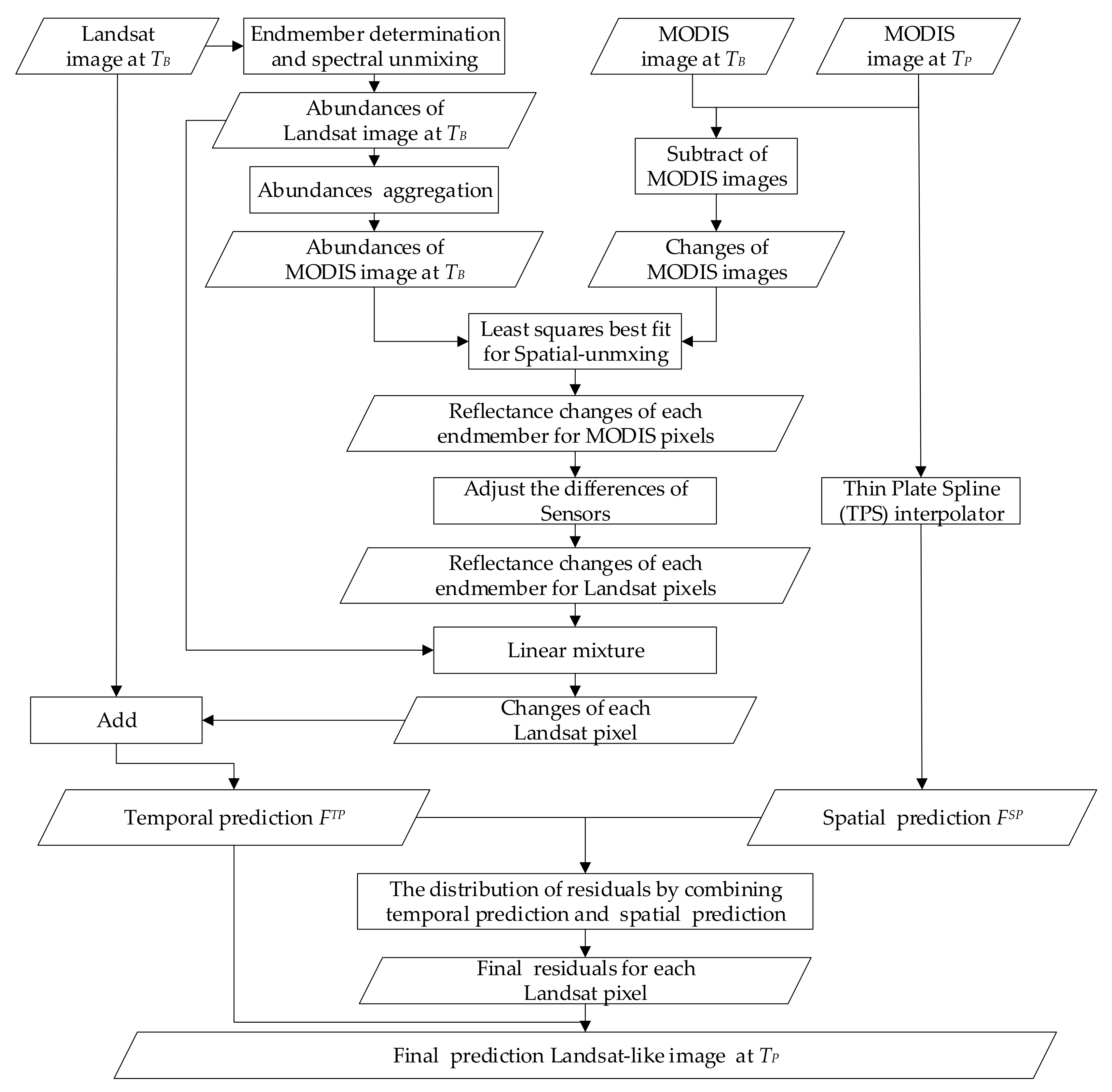
2.2. Theoretical Basis of EFSDAF

Like FSDAF, the input images of EFSDAF include, a MODIS image at $T_B$, a Landsat image at $T_B$ and a MODIS image at $T_P$. The output of EFSDAF is a predicted fine resolution image (e.g., Landsat-like) at $T_P$. Unlike FSDAF, EFSDAF considers more than one land cover type in both the Landsat images (30 m) and MODIS images (500 m). Therefore, the endmembers determination and abundances extraction of the Landsat image at $T_B$ are firstly carried out in EFSDAF. EFSDAF includes five main steps: (1) endmember determination and spectral unmixing for Landsat image at $T_B$; (2) temporal prediction ($F^{TP}$) for no land cover change from $T_B$ to $T_P$; (3) spatial prediction ($F^{SP}$) for land cover change at $T_P$; (4) residual distribution by using a new residual index (RI); and (5) final prediction of a Landsat-like image using neighborhood in a sliding window. The workflow of EFSDAF is outlined by the flowchart in Figure 1. Detailed descriptions of each step in EFSDAF are given below. The code of EFSDAF can be found at the URL https://github.com/max19951001/EFSDAF.git.

2.2.1. Endmember Determination and Spectral Unmixing for Landsat Images at $T_B$

Endmember extraction and spectral unmixing of Landsat images at $T_B$ are the first step and key step for EFSDAF in this paper due to the heterogeneity of land surface with more than one land cover type in Landsat pixels. In this study, a globally representative spectral linear mixture model (SVD model) [34,35,36] shared by Small for Landsat images was selected as endmembers that were classified into three types: substrate (S), vegetation (V), and dark surface (D) [20], and as a linear method, the fully constrained least squares (FCLS) [37] method was applied to the spectral unmixing. The abundance $A_F^B\left(x_{ij},y_{ij},m\right)$ calculated by FCLS varies from 0 to 1, and the sum of $A_F^B\left(x_{ij},y_{ij},m\right)$ is 1.

2.2.2. Temporal Prediction ($F^{TP}$ ) for No Land Cover Change from $T_B$ to $T_P$

• Temporal changes of each endmember at the MODIS pixels

The temporal prediction of EFSDAF assumes no land cover change from $T_B$ to $T_P$. In other words, the endmembers and abundances of Landsat pixels will not change from $T_B$ to $T_P$. According to the linear mixture model [38], the values of Landsat pixels are a linear mixture of endmembers’ values and abundances. Hence, the values of Landsat pixels at $T_B$ and $T_P$ can be expressed as:

$$\begin{array}{c}{F}_B\left(x_{ij},y_{ij},b\right)={\displaystyle {\displaystyle \sum }_{m=1}^{n_m}}{A}_F^B\left(x_{ij},y_{ij},m\right)\times R_F^B\left(m,b\right)+\phi \end{array}$$

(1)

$$\begin{array}{c}{F}_p\left(x_{ij},y_{ij},b\right)={\displaystyle {\displaystyle \sum }_{m=1}^{n_m}}{A}_F^p\left(x_{ij},y_{ij},m\right)\times R_F^p\left(m,b\right)+\phi \end{array}$$

(2)

where $n_m$ defines the number of endmembers and m is the m-th endmembers for one Landsat pixel, $R_F^B\left(m,b\right)$ and $R_F^P\left(m,b\right)$ denote the reflectance values of each endmember for all Landsat image bands at $T_B$ and $T_P$, respectively. $\phi$ is the system error. According to the above assumption, the endmembers and abundances of Landsat pixels will not change from $T_B$ to $T_P$, i.e., $A_F^B$ = $A_F^P$, and $\phi$ is constant. From Equations (1) and (2), we have:

$$\begin{array}{c}\Delta F\left(x_{ij},y_{ij},b\right)={\displaystyle {\displaystyle \sum }_{m=1}^{n_m}}{A}_F^B\left(x_{ij},y_{ij},m\right)\times \Delta R_F\left(m,b\right)\end{array}$$

(3)

where $\Delta F$ denotes the temporal changes of the Landsat images. $\Delta R_F$ are the reflectance changes of each endmember for all Landsat image bands. Among the variables above, if $\Delta R_F$ is known, $\Delta F$ can be calculated by a linear mixture model. Therefore, the key is to solve $\Delta R_F$.

Similar to the temporal changes of Landsat images, the temporal changes of MODIS images from $T_B$ to $T_P$ can be expressed as:

$$\begin{array}{c}\Delta C\left(x_i,y_i,b\right)={\displaystyle {\displaystyle \sum }_{m=1}^{n_m}}{A}_C^B\left(x_i,y_i,m\right)\times \Delta R_C\left(m,b\right).\end{array}$$

(4)

where $\Delta C$ denotes the temporal changes of the MODIS images. $\Delta R_C$ are the reflectance changes of each endmember for all MODIS image bands. Among the variables above, $\Delta C$ could be calculated through $\Delta C=C_P-C_B$. Due to the previous assumption of no land cover change from $T_B$ to $T_P$, the types and spatial distributions of the endmembers should be the same for Landsat and MODIS images in the same regions. Hence, $A_C^B$ can be aggregated from $A_F^B$ with:

$$\begin{array}{c}{A}_C^B\left(x_i,y_i,m\right)=\frac{1}{s^2}{\displaystyle {\displaystyle \sum }_{k=1}^{s2}}{A}_F^B\left(x_{ij},y_{ij},m\right)\end{array}$$

(5)

where $A_C^B\left(x_i,y_i,m\right)$ is calculated by averaging the endmember abundances of all Landsat pixels in one MODIS pixel. However,$A_C^B\left(x_i,y_i,m\right)$ is the ratio of the number of Landsat pixels for class $m$ to $s^2$ in FSDAF. Although $\Delta C\left(x_i,y_i,b\right)$ and $A_C^B\left(x_i,y_i,m\right)$ from Equations (4) and (5) are known variables, Equation (4) cannot be solved because there are $n_m$ unknown values of $\Delta R_C\left(m,b\right)$.

In this study, assuming that the land cover types are the same for a small area according to the first law of geography [39] stating that near things are more related than distant things, it is reasonable that $\Delta R_C\left(m,b\right)$ are the same in a small area [20]. However, FSDAF assumes that the temporal changes of each class are the same among all MODIS pixels, which does not match the actual situation. A sliding window of MODIS pixels is introduced to perform spatial unmixing in this study, and the size of the window should be larger than the number of endmembers [40]. The equations [32] are as follows:

$$\left(\begin{array}{c}\Delta C\left(x_1,y_1,b\right)\\ ⋮\\ \Delta C\left(x_i,y_i,b\right)\\ ⋮\\ \Delta C\left(x_n,y_n,b\right)\end{array}\right)=\left(\begin{array}{c}{A}_C^B\left(x_1,y_1,1\right) A_C^B\left(x_1,y_1,2\right) \cdots A_C^B\left(x_1,y_1,m\right)\\ ⋮ ⋮ ⋮ \\ A_C^B\left(x_i,y_i,1\right) A_C^B\left(x_i,y_i,2\right) \cdots A_C^B\left(x_i,y_i,m\right)\\ ⋮ ⋮ ⋮ \\ A_C^B\left(x_n,y_n,1\right) A_C^B\left(x_n,y_n,2\right) \cdots A_C^B\left(x_n,y_n,m\right)\end{array}\right)\left(\begin{array}{c}\Delta R_C\left(1,b\right)\\ ⋮\\ \Delta R_C\left(l,b\right)\\ ⋮\\ \Delta R_C\left(m,b\right)\end{array}\right)$$

(6)

where $\Delta R_C\left(m,b\right)$ can be calculated by computing a least squares best fit solution. Selecting k of the purest MODIS pixels of each endmember in the sliding window for least squares best fit aims to reduce the errors by collinearity [32]. The final determined MODIS pixels for least squares best fit should be smaller than the size of the sliding window and larger than the number of endmembers.

• Adjustment of the differences between the Landsat images and MODIS images

Theoretically speaking, the reflectance values of the Landsat pixels corresponding to the MODIS pixels are the same. However, due to the physical differences of the sensors, the effects of bandwidth, weather conditions, and atmospheric correction, differences between MODIS images and Landsat images are inevitable. As with previous studies [20,41], a linear model is introduced in this study to adjust the differences between Landsat images and MODIS images.

$$\begin{array}{c}{R}_F^B\left(m,b\right)=a_1\left(b\right)\times R_C^B\left(m,b\right)+b_1\end{array}$$

(7)

$$\begin{array}{c}{R}_F^P\left(m,b\right)=a_1\left(b\right)\times R_C^P\left(m,b\right)+b_1\end{array}$$

(8)

where $a_1\left(b\right)$ and $b_1$ are the slope and interception of the linear model, respectively. From Equations (7) and (8), the differences between $\Delta R_C\left(m,b\right)$ and $\Delta R_F\left(m,b\right)$ can be calculated as the following Equation (9).

$$\begin{array}{c}\Delta R_F\left(m,b\right)=a_1\left(b\right)\times \Delta R_C\left(m,b\right)\end{array}$$

(9)

$\Delta R_F\left(m,b\right)$ can be obtained from Equations (5)–(9) in this study. However, the $\Delta R_F\left(m,b\right)$ of FSDAF were calculated by assigning the temporal changes of MODIS images to Landsat images without considering the differences of Landsat and MODIS images.

• Temporal prediction for the fine resolution image at $T_P$

$\Delta F$ is linearly mixed with $A_F^B$ from Equation (3), and the final temporal prediction can be calculated by Equation (10) as follows:

$$\begin{array}{c}{F}^{TP}\left(x_{ij},y_{ij},b\right)=F_B\left(x_{ij},y_{ij},b\right)+\Delta F\left(x_{ij},y_{ij},b\right)\end{array}$$

(10)

Although the final temporal prediction can be calculated by Equation (10), all of the above calculations are based on the assumption of no land cover change from $T_B$ to $T_P$. Hence, the temporal prediction cannot accurately predict abrupt change events from $T_B$ to $T_P$. In addition, because this prediction only uses the information of the temporal changes between $T_B$ and $T_P$, we call Section 2.2.2 the temporal prediction.

2.2.3. Spatial Prediction ($F^{SP}$) for Land Cover Change at $T_P$

• Analysis and calculation of the residual

The temporal prediction from Section 2.2.2 is not an accurate prediction when there are land cover changes. Specifically, there is a certain deviation between the true values ($F_p$) and the temporal prediction values ($F^{TP}$). This study introduces a residual R between the $F_P$ and the $F^{TP}$ as follows:

$$\begin{array}{c}\frac{1}{S^2}{\displaystyle {\displaystyle \sum }_{s=1}^{s^2}}{F}_P\left(x_{ij},y_{ij},b\right)=\frac{1}{S^2}{\displaystyle {\displaystyle \sum }_{s=1}^{s^2}}{F}^{TP}\left(x_{ij},y_{ij},b\right)+R\left(x_i,y_i,b\right)\end{array}$$

(11)

Furthermore, the value of one MODIS pixel is equal to the average of all of Landsat pixels within one MODIS pixels and a system deviation $\phi$ [7]. Hence, the values of MODIS pixels at $T_B$ and $T_P$ can be expressed as:

$$\begin{array}{c}{C}_B\left(x_i,y_i,b\right)=\frac{1}{ s^2}{\displaystyle {\displaystyle \sum }_{s=1}^{s^2}}{F}_B\left(x_{ij},y_{ij},b\right)+\phi \end{array}$$

(12)

$$\begin{array}{c}{C}_P\left(x_i,y_i,b\right)=\frac{1}{s^2}{\displaystyle {\displaystyle \sum }_{s=1}^{s^2}}{F}_P\left(x_{ij},y_{ij},b\right)+\phi \end{array}$$

(13)

From Equations (11)–(13), we have:

$$\begin{array}{c}R\left(x_i,y_i,b\right)=\Delta C\left(x_i,y_i,b\right)-\frac{1}{S^2}\left[{\displaystyle {\displaystyle \sum }_{s=1}^{s^2}}{F}^{TP}\left(x_{ij},y_{ij},b\right)-{\displaystyle {\displaystyle \sum }_{s=1}^{s^2}}{F}_B\left(x_{ij},y_{ij},b\right)\right]\end{array}$$

(14)

As can be seen from the above Equations (11)–(14), the calculation and distribution of the residual R is a key step for obtaining the final prediction at $T_P$.

• Spatial prediction of the MODIS image at $T_P$

As described above, the source of the residual R is in the area of land cover change. However, the information of land cover change can only be obtained from the MODIS image at $T_P$. Therefore, downscaling the MODIS image to Landsat image level is the vital step to obtain the information of the land cover change at $T_P$. In EFSDAF, a Thin Plate Spline (TPS) interpolation method is applied to downscale the MODIS image at $T_P$. TPS is a spatial interpolation technique for point data based on spatial dependence [42], which was used to the spatiotemporal fusion method because it has high interpolation accuracy [32,43]. The interpolation result of the MODIS image at $T_P$ will be marked as $F_P^{SP}\left(x_{ij},y_{ij},b\right)$, which is another prediction of the Landsat image at $T_P$. Unlike FSDAF, the MODIS image at $T_B$ is also interpolated using the TPS method to calculate the residual index (RI) in Section 2.2.4 for EFSDAF, and its result will be marked as $F_B^{SP}\left(x_{ij},y_{ij},b\right)$. Because the spatial information is obtained from MODIS images using the TPS interpolator method, we call Section 2.2.3 spatial prediction.

2.2.4. Residual Distribution by Using a New Residual Index (RI)

From Equation (11), the predicted Landsat-like image is calculated by adding a reasonable residual based on the temporal prediction. Therefore, the residual distribution is the key step for the final prediction. In FSDAF, a homogeneity index (HI) derived from the classification map of the Landsat image at $T_B$ was introduced to guide the residual distribution. Because the HI only depends on the classification map at $T_B$, it will be unreasonable when the land cover type has changed from $T_B$ to $T_P$ or the classification map is wrong [33]. Hence, a new residual index (RI) is proposed to reasonably guide the residual distribution in this study, and more residual will be assigned to the area of land cover change. According to Section 2.2.3, the spatial variation $\Delta F_{BP}\left(x_{ij},y_{ij},b\right)$ can be expressed as:

$$\begin{array}{c}\Delta F_{BP}\left(x_{ij},y_{ij},b\right)=\left|F_P^{SP}\left(x_{ij},y_{ij},b\right)-F_B^{SP}\left(x_{ij},y_{ij},b\right)\right|\end{array}$$

(15)

where $\Delta F_{BP}\left(x_{ij},y_{ij},b\right)$ defines the changes of interpolation results of MODIS images from $T_B$ to $T_P$, and the larger $\Delta F_{BP}\left(x_{ij},y_{ij},b\right)$, the larger the changes of land cover type. In EFSDAF, we assume the changes of land cover type occur in a small area. If $\Delta F_{BP}\left(x_{ij},y_{ij},b\right)$ in one Landsat pixel is greater than the average of the $\Delta F_{BP}$, and we think the Landsat pixel $\left(x_{ij},y_{ij}\right)$ is the area of land cover change. The RI can be calculated as follows:

$$\begin{array}{c}RI\left(x_{ij},y_{ij},b\right)=\frac{{{\displaystyle \sum }}_{k=1}^n{I}_k}{n_w}\end{array}$$

(16)

where $I_k$ is equal to 1 when the k-th Landsat pixels is determined to the pixel of land cover change within a sliding window; otherwise, $I_k$ is equal to 0. $n_w$ defines the window size. The RI is the ratio of the numbers of $I_k$ = 1 in the window to $n_w$. The range of RI is 0–1, and a larger RI indicates more residual to the area of land cover change.

Then we use the same weighting function to distribute the final residual as FSDAF. The weighting function is defined as follow:

$$\begin{array}{c}CW\left(x_{ij},y_{ij},b\right)=E_{he}\left(x_{ij},y_{ij},b\right)\times RI\left(x_{ij},y_{ij},b\right)+E_{ho}\left(x_{ij},y_{ij},b\right)\times \left(1-RI\left(x_{ij},y_{ij},b\right)\right)\end{array}$$

(17)

where $E_{he}\left(x_{ij},y_{ij},b\right)$ = $R\left(x_i,y_i,b\right)$, and $E_{he}\left(x_{ij},y_{ij},b\right)$ is the residual for the area of land cover change. $E_{ho}\left(x_{ij},y_{ij},b\right)=F_P^{SP}\left(x_{ij},y_{ij},b\right)-F^{TP}\left(x_{ij},y_{ij},b\right)$, and $E_{ho}\left(x_{ij},y_{ij},b\right)$ is the residual for area of no land cover change.

The final residual $r\left(x_{ij},y_{ij},b\right)$ can be calculated as follows:

$$\begin{array}{c}r\left(x_{ij},y_{ij},b\right)=s^2\times R\left(x_i,y_i,b\right)\times W\left(x_{ij},y_{ij},b\right)\end{array}$$

(18)

where $W\left(x_{ij},y_{ij},b\right)$ is the normalized $CW\left(x_{ij},y_{ij},b\right)$.

According to Equations (10) and (11), the final changes of the Landsat images between $T_B$ and $T_P$ can be obtained from Equation (19):

$$\begin{array}{c}\Delta F_f\left(x_{ij},y_{ij},b\right)=r\left(x_{ij},y_{ij},b\right)+\Delta F\left(x_{ij},y_{ij},b\right)\end{array}$$

(19)

where $\Delta F_f\left(x_{ij},y_{ij},b\right)$ and $\Delta F\left(x_{ij},y_{ij},b\right)$ are the final changes of Landsat images and the changes of temporal prediction from $T_B$ to $T_P$, respectively.

2.2.5. Final Prediction of the Landsat-Like Image Using Neighborhood in a Sliding Window

Theoretically, the final prediction of Landsat-like image $F_{tp}\left(x_{ij},y_{ij},b\right)$ at $T_P$ can be obtained by the following equation.

$$\begin{array}{c}{F}_{tp}\left(x_{ij},y_{ij},b\right)=F_B\left(x_{ij},y_{ij},b\right)+\Delta F_f\left(x_{ij},y_{ij},b\right)\end{array}$$

(20)

However, uncertain errors are inevitable in EFSDAF because of the complexity of the calculation process and the characteristics of pixel-by-pixel. In addition, the final prediction will lead to block effects because the residual distribution is for the MODIS pixels. In this study, EFSDAF adopts the same solution as STARFM, which uses the information of neighborhood to reduce the uncertainties and smooth final prediction in a sliding window. The final predicted Landsat-like image $F_{fp}\left(x_{ij},y_{ij},b\right)$ can be calculated by Equation (21), and detailed information can be found in STARFM [7].

$$\begin{array}{c}{F}_{fp}\left(x_{ij},y_{ij},b\right)=F_B\left(x_{ij},y_{ij},b\right)+{\displaystyle {\displaystyle \sum }_{k=1}^n}{w}_k\times \Delta F_f\left(x_{ij},y_{ij},b\right)\end{array}$$

(21)

where n is the number of similar pixels for Landsat pixels in a sliding window, and $w_k$ is the weight for each similar pixel.

3. Testing Experiment

3.1. Study Area and Data

The EFSDAF is proposed to accurately monitor dynamic changes of land surface including gradual change (e.g., vegetation phenology) and abrupt change events (e.g., flood). In this study, vegetation phenology and flood events are selected to evaluate the performance of EFSDAF.

The selected two datasets were from the datasets shared by Emelyanova [10], which were collected in the Lower Gwydir Catchment in Northern New South Wales, Australia (149.2815° E, 29.0855° S, hereinafter called “Gwydir”) and have been widely applied in the evaluation of spatiotemporal fusion methods [10,20,21,32,44]. All images were atmospherically corrected and geographically co-registered, which was resampled to 25 m with the nearest neighbor method by Emelyanova. In EFSDAF, we aggregated the MODIS pixels to 500 m resolution in the process of residual distribution. Two pairs of Landsat and MODIS images of the first dataset (vegetation phenology) were acquired on 5 July 2004 and 6 August 2004 in Gwydir, and the size of the selected images is $1400\times 1400 \mathrm{pixels}$. The first dataset was a typical heterogeneous region, and temporal dynamic changes were mainly caused by phenological change from 5 July to 6 August 2004. The selected Landsat and MODIS images of the first dataset are shown in Figure 2. The second dataset (flood) was acquired on 11 November 2004 and 12 December 2004, and the size of selected images is 800 × 800 pixels. A large flood occurred from 26 November 2004 to 12 December 2004, and the dataset was a typical abrupt change area. The selected Landsat and MODIS images of the second dataset are shown in Figure 3.

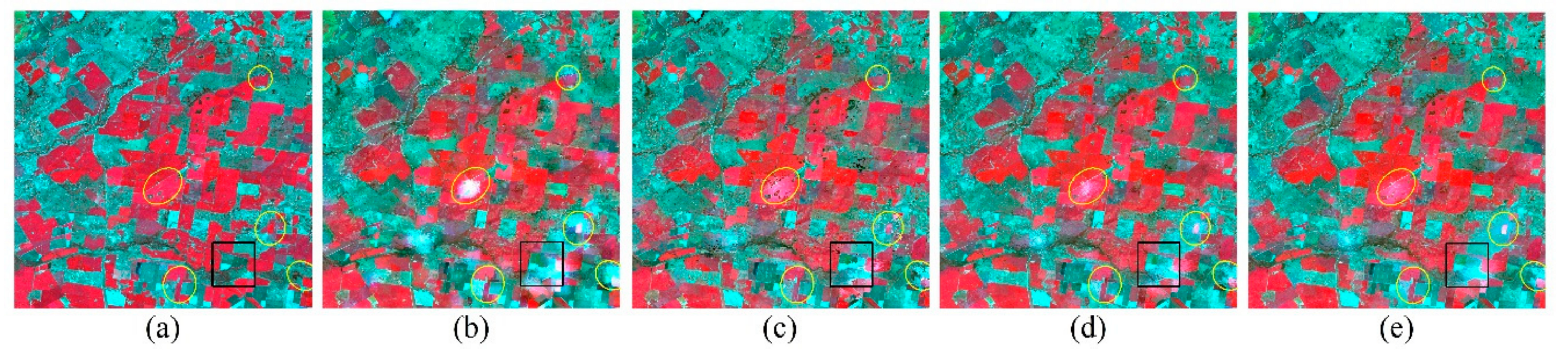
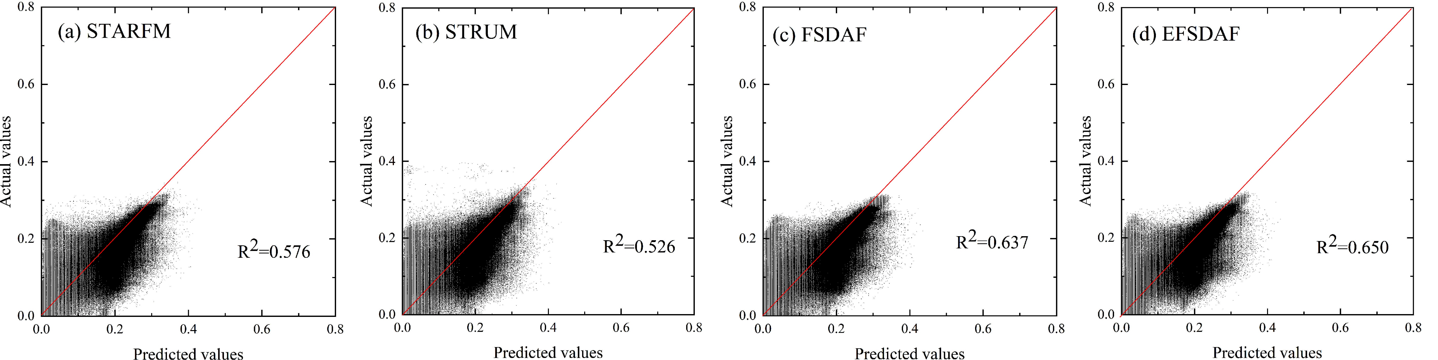
3.2. Comparison and Evaluation of EFSDAF with STARFM, STRUM, and FSDAF

In this study, we compared EFSDAF with three other fusion methods: STARFM, STRUM, and FSDAF. Because these three fusion methods have been widely used, and each of them only needs one pair of Landsat and MODIS images at $T_B$ and one MODIS image at $T_P$ as input data.

All fusion images are qualitatively and quantitatively evaluated by comparing the predicted Landsat-like image with true images at $T_P$. The qualitative evaluation is to visually compare the predicted images with the true images, and the differences between the predicted images of the four fusion methods are magnified and highlighted by using yellow elliptical circles and black squares. Representative assessment indexes as quantitative evaluation are used to objectively evaluate the predicted images and true images pixel by pixel, and they are Average Difference (AD), Root Mean Square Error (RMSE), Correlation Coefficient (CC), and Structure Similarity (SSIM) [45], respectively. The evaluation criteria are as follows: the closer AD and RMSE are to 0, the closer the predicted value to the true value; the closer CC and SSIM are to 1, the more similar the predicted images are to the true images.

4. Results

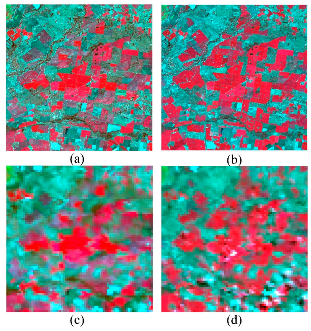
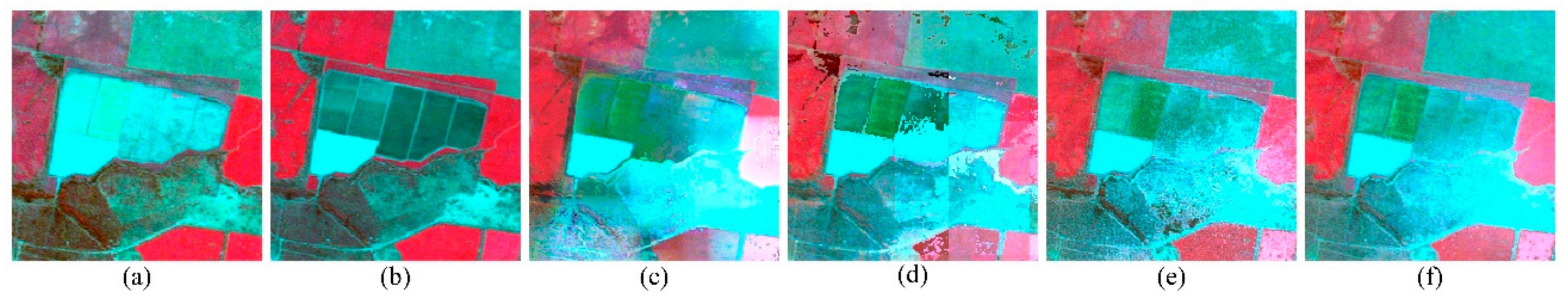
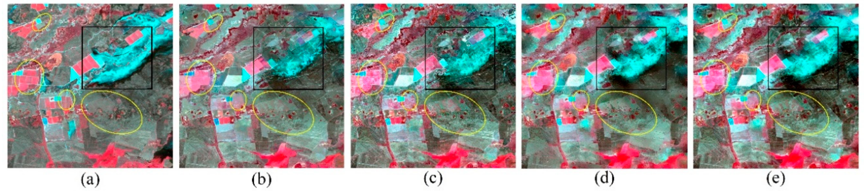
4.1. Experiment in Gradual Change Area (Vegetation Phenology)

From Figure 4, the predicted Landsat-like images by four methods can monitor the changes of vegetation growth, and the results of the four fusion methods are similar to the true image on the whole. However, the yellow elliptical circles in Figure 4 show the differences of the four methods, and we can get that STARFM blurs the boundaries of different objects, STRUM produces block effects, FSDAF cannot retain the spatial details, and EFSDAF is closest to the true image. Especially, EFSDAF can accurately retain the boundaries of objects from Figure 5, and it can capture more spatial details of the object than FSDAF.

From quantitative indices of four methods in

Table 1. The quantitative assessment of the Landsat-like images by STARFM, STRUM, FSDAF, and EFSDAF in dataset 1.

		STARFM	STRUM	FSDAF	EFSDAF
AD	B1	0.0267	0.0264	0.0262	0.0260
	B2	0.0205	0.0203	0.0197	0.0197
	B3	0.0176	0.0182	0.0169	0.0167
	B4	0.0442	0.0480	0.0385	0.0379
	B5	0.0244	0.0237	0.0233	0.0209
	B7	0.0250	0.0266	0.0237	0.0226
	Mean	0.0264	0.0272	0.0247	0.0225
RMSE	B1	0.0319	0.0299	0.0295	0.0284
	B2	0.0270	0.0250	0.0245	0.0229
	B3	0.0249	0.0244	0.0232	0.0212
	B4	0.0588	0.0646	0.0542	0.0504
	B5	0.0329	0.0322	0.0310	0.0270
	B7	0.0341	0.0363	0.0322	0.0297
	Mean	0.0349	0.0354	0.0324	0.0299
CC	B1	0.653	0.732	0.778	0.803
	B2	0.724	0.781	0.812	0.845
	B3	0.852	0.869	0.895	0.915
	B4	0.891	0.850	0.897	0.914
	B5	0.856	0.871	0.880	0.918
	B7	0.865	0.853	0.886	0.905
	Mean	0.807	0.826	0.858	0.883
SSIM	B1	0.504	0.575	0.617	0.632
	B2	0.683	0.744	0.798	0.804
	B3	0.836	0.852	0.865	0.890
	B4	0.885	0.848	0.893	0.902
	B5	0.854	0.869	0.887	0.908
	B7	0.862	0.848	0.881	0.892
	Mean	0.771	0.789	0.823	0.839

, the fusion results by four methods can achieve high accuracy. For all six bands and the mean, it can be seen that the accuracy of EFSDAF is the highest by comparing it with the other three methods, which have lower AD and RMSE, as well as higher CC and SSIM. Taking the mean of all bands as an example, the CC values of the four methods are 0.807, 0.826, 0.858, and 0.883 from left to right, respectively. In addition, because the vegetation phenology change happened in dataset 1, the prediction accuracy of band 4 (NIR) can better illustrate the performance of the four methods. From the scatter plot of Figure 6, it can be confirmed that the synthetic image values by EFSDAF are closer to the true values than the other three methods.

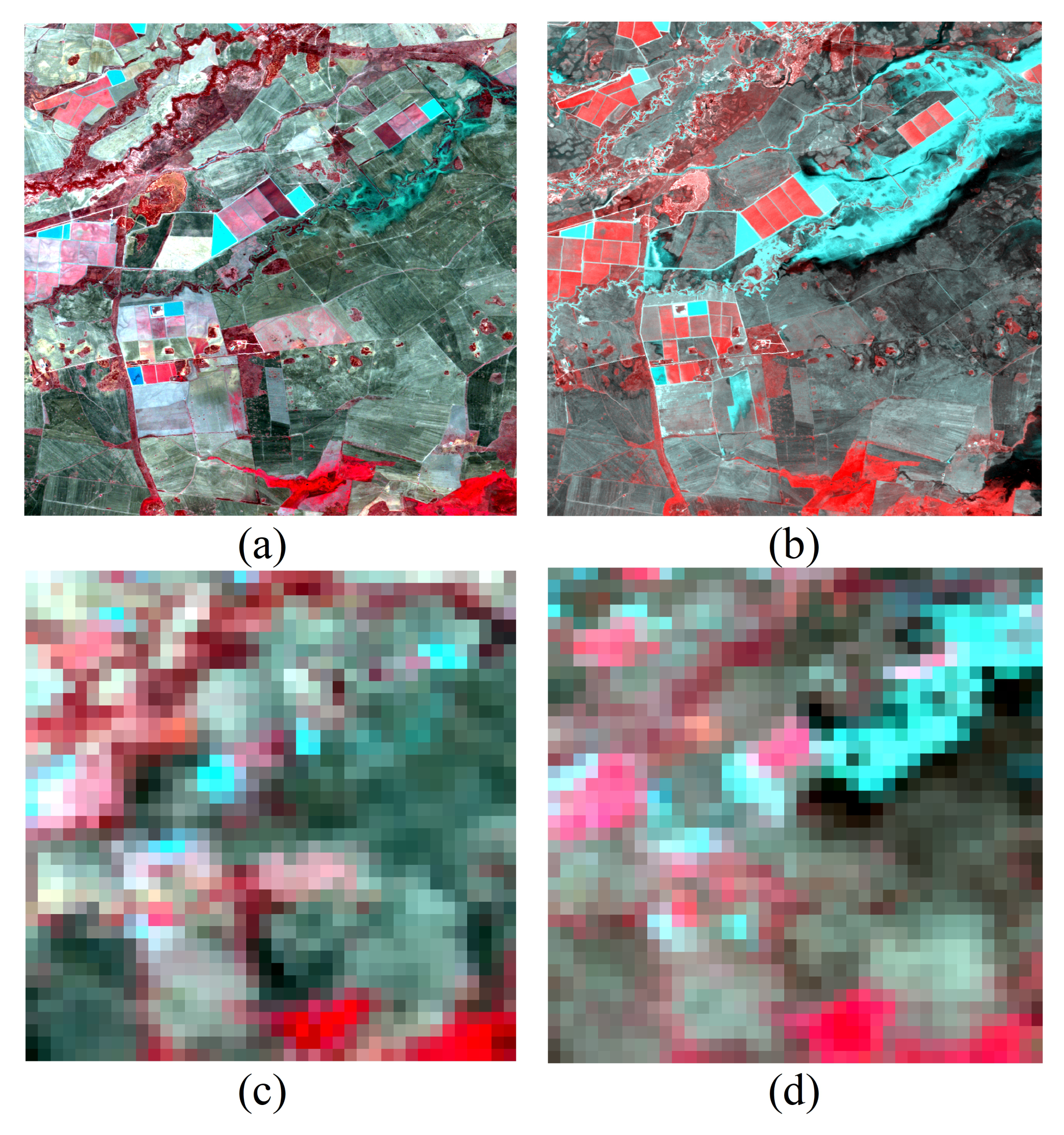
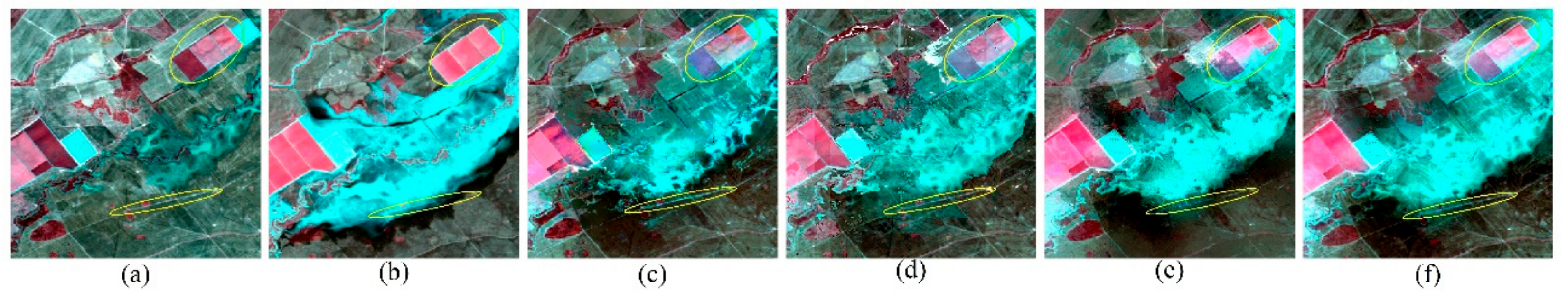
4.2. Experiment in Abrupt Change Area (Flood)

From the visual comparison, only FSDAF and EFSDAF can capture the information of land cover change in Figure 7, it can be more clearly and accurately seen from the zoom-in black area in Figure 8. In addition, the spatial details restored by EFSDAF are most complete and most similar with the true image from the yellow elliptical circles of Figure 7. From the yellow elliptical circles of Figure 8, the small flood change information can be accurately captured by EFSDAF, but it cannot be captured by FSDAF.

Comparing the results of the quantitative indices in

Table 2. Quantitative assessment of the Landsat-like images by STARFM, STRUM, FSDAF, and EFSDAF in dataset 2.

		STARFM	STRUM	FSDAF	EFSDAF
AD	B1	0.0104	0.0104	0.0096	0.0094
	B2	0.0137	0.0141	0.0130	0.0127
	B3	0.0165	0.0167	0.0155	0.0151
	B4	0.0249	0.0259	0.0238	0.0227
	B5	0.0487	0.0520	0.0423	0.0425
	B7	0.0444	0.0472	0.0394	0.0392
	Mean	0.0264	0.0277	0.0239	0.0235
RMSE	B1	0.0152	0.0145	0.0137	0.0136
	B2	0.0214	0.0207	0.0196	0.0193
	B3	0.0260	0.0249	0.0236	0.0231
	B4	0.0364	0.0371	0.0342	0.0326
	B5	0.0643	0.0685	0.0560	0.0560
	B7	0.0560	0.0595	0.0505	0.0502
	Mean	0.0366	0.0375	0.0329	0.0324
CC	B1	0.595	0.617	0.654	0.667
	B2	0.607	0.628	0.665	0.672
	B3	0.594	0.626	0.663	0.674
	B4	0.789	0.771	0.808	0.827
	B5	0.759	0.725	0.785	0.791
	B7	0.743	0.710	0.752	0.763
	Mean	0.681	0.679	0.721	0.733
SSIM	B1	0.583	0.611	0.644	0.645
	B2	0.577	0.613	0.643	0.653
	B3	0.565	0.610	0.642	0.648
	B4	0.778	0.761	0.796	0.815
	B5	0.748	0.714	0.768	0.772
	B7	0.705	0.669	0.714	0.719
	Mean	0.659	0.663	0.701	0.709

, STARFM and STRUM present similar results, and EFSDAF is better than FSDAF (CC 0.808 vs. 0.827, SSIM 0.796 vs. 0.815 for band 4). Furthermore, since the water body information shows lower reflectivity for band 4 (NIR), we compare the scatter plots of band 4 for the four methods in Figure 9. It can be concluded that FSDAF and EFSDAF are far superior to STARFM and STRUM, and EFSDAF is better than FSDAF.

5. Discussion

The proposed EFSDAF method in this paper was an improvement on FSDAF. EFSDAF considered the mixed pixels of both Landsat images and MODIS images, and it predicted the Landsat-like images by combining spectral unmixing analysis and TPS interpolator. The experiment results showed that the fusion results by EFSDAF were better than FSDAF.

5.1. Improvements of EFSDAF Compared with FSDAF

The fusion results of EFSDAF were better than FSDAF due to the following reasons. Firstly, EFSDAF considered the mixed pixels phenomenon of the fine resolution image (e.g., Landsat), which was the most significant improvement of EFSDAF. In this study, the SVD model was introduced to perform the spectral unmixing by using a fully constrained least squares method. Moreover, the abundances of MODIS pixels were calculated by averaging the abundances of all Landsat pixels in one MODIS pixel, and the final changes of Landsat images were solved by a linear mixture that combined the abundances of endmembers and the variations of endmembers for Landsat images from $T_B$ to $T_p$. Hence, the proposed EFSDAF considered the intra-class variability, and it can reserve more spatial details than FSDAF, which can be seen in the yellow elliptical circles of Figure 4 and Figure 7. Secondly, the spatial unmixing of the coarse resolution image (e.g., MODIS) was performed in a sliding window, which was different from the spatial unmixing of FSDAF using the whole MODIS image. It was more in line with the actual situation by using sliding windows for spatial unmixing due to the heterogeneity of land surface. The size of the sliding window for spatial unmixing was recommended to $7\times 7$ MODIS pixels because the fusion accuracy is the best. Furthermore, selecting k purest MODIS pixels of a sliding window for spatial unmixing ensured the minimal impacts of collinearity [32]. Thirdly, the differences between the Landsat and MODIS images were considered, which included the differences of the sensors and the pre-processing errors. In this study, we used a linear model to adjust the differences between the Landsat and MODIS images, but FSDAF did not consider the differences. Finally, a new residual index (RI) was introduced to guide the residual distribution instead of the homogeneity index (HI) of FSDAF. The HI will not be suitable to guide the residual distribution when there are land cover changes or misclassification [33] because it was calculated from the classification map at $T_B$. The proposed RI adequately considered the source of the errors, and it was based on the differences of the interpolator results between the MODIS image at $T_B$ and the MODIS image at $T_P$. Greater differences represent more significant land cover change and will have a larger RI value. The RI was calculated in a sliding window, and the size of the window should not be too large because the result will not be accurate for the edge of different land cover types. The recommended size was $51\times 51$ Landsat pixels according to Section 2.2.5 in this study. More information of land cover change can be monitored by EFSDAF from the yellow elliptical circles in Figure 8e,f. In addition, EFSDAF is an automated fusion method compared to FSDAF because additional input parameters were not required.

5.2. Influence of Endmember Variability on EFSDAF

The endmember variability directly affected the abundances of the Landsat image which may further affect the final fusion precision of EFSDAF. Hence, we evaluated the performance of EFSDAF by using different endmember numbers. In this study, the SVD model shared by Small and 3~5 endmembers extracted from the Landsat image at $T_B$ were selected to test the influence of endmember variability on EFSDAF, and the final results of the two datasets were shown in

Table 3. The fusion precision of EFSDAF by using different endmember numbers in two datasets (NIR-red-green).

		Dataset 1				Dataset 2
Endmember		SVD	3	4	5	SVD	3	4	5
AD	Green	0.0197	0.0198	0.0197	0.0198	0.0127	0.0128	0.0130	0.0130
	Red	0.0167	0.0168	0.0168	0.0168	0.0151	0.0152	0.0156	0.0156
	NIR	0.0379	0.0390	0.0381	0.0374	0.0227	0.0227	0.0230	0.0236
RMSE	Green	0.0229	0.0229	0.0229	0.0230	0.0193	0.0193	0.0197	0.0197
	Red	0.0212	0.0213	0.0213	0.0213	0.0231	0.0232	0.0236	0.0238
	NIR	0.0504	0.0504	0.0496	0.0490	0.0326	0.0327	0.0331	0.0336
CC	Green	0.845	0.845	0.846	0.843	0.672	0.674	0.656	0.657
	Red	0.915	0.914	0.914	0.914	0.674	0.675	0.659	0.650
	NIR	0.914	0.914	0.915	0.918	0.827	0.827	0.822	0.815
SSIM	Green	0.804	0.804	0.805	0.802	0.653	0.645	0.625	0.626
	Red	0.890	0.889	0.889	0.889	0.648	0.647	0.635	0.618
	NIR	0.902	0.902	0.906	0.908	0.815	0.815	0.810	0.800

below (three bands for testing, NIR-red-green). As can be seen from Table 3, the predicted results of EFSDAF using four different endmembers are close in the two datasets. Therefore, the influence of endmember variability on the final fusion results can be negligible, and EFSDAF is robust to endmember variability. For the automated operation of EFSDAF, the SVD model of Landsat image was used to perform the spectral unmixing in this study.

5.3. The Effect of Input Images on the Predicted Values of EFSDAF

Like FSDAF, the minimum input images were used to predict the final Landsat-like images in EFSDAF. Hence, the fusion accuracy of EFSDAF was directly influenced by the input images [10,19]. Particularly, the spatial information and temporal information of the input images would be fully utilized in EFSDAF. Figure 10 showed the differences between the predicted Landsat-like image of EFSDAF and input images in dataset 2. From Figure 10b–d, it can be seen that the land cover type has changed, and the information of land cover change can be captured by comparing Figure 10b with Figure 10c. However, there was an obvious difference between the predicted image in the yellow ellipse area of Figure 10b and the true image (Figure 10a). After comparing and analyzing the input images and the predicted image in Figure 10a,d, it can be concluded that the input MODIS image at $T_P$ lacks the information of land cover change in the yellow ellipse from Figure 10c; therefore, the final predicted image in Figure 10a was different from the true image at $T_P$ from Figure 10a. However, comparing the abrupt change area of MODIS images from $T_B$ to $T_P$ in Figure 10c,d, EFSDAF can completely capture the spatial details in Figure 10b. In other words, EFSDAF can only accurately monitor the information of abrupt change in MODIS images. Hence, the quality of the input images is crucial to the fusion accuracy of EFSDAF.

5.4. Applications of EFSDAF to other Remote Sensing Products and Sensors

The EFSDAF in this study was tested using surface reflectance values of MODIS and Landsat images, but the purpose of EFSDAF is to study various complex surface dynamics. Therefore, EFSDAF can be applied to vegetation monitoring (e.g., NDVI), crop growth, and other sudden events such as urbanization, forest fires, and landslides. In addition, with the frequent launch of satellites for the Earth Observation System in recent years, existing satellite sensors such as Sentinel 2 MSI (10, 20, 60 m) images can replace Landsat images as fine resolution images, and like Sentinel 3 OLCI (300 m), NPP-VIIRS images (375/750 m) can replace MODIS images as coarse resolution images. We are looking forward to testing EFSDAF for other applications as well as satellite sensors.

5.5. Limitations of EFSDAF

EFSDAF can predict both gradual change and abrupt change events, but it cannot accurately monitor tiny changes (e.g., small flood information in this study) because tiny changes are not shown in one MODIS pixel. In other words, the changes of $20\times 20$ Landsat pixels can be displayed in one MODIS pixel in this study. Therefore, the prediction accuracy of tiny changes can be improved by blending Landsat images (30 m) and Sentinel 3 OLCI images (300 m), but the predicted images still cannot monitor all actual changes. In addition, the computational efficiency of EFSDAF is the slowest compared with other three methods due to the complexity of the calculation process. However, the computational efficiency of fusion methods will be ignored in the future with the rapid development of high-performance computing platforms like Google Earth Engine (GEE) [46].

6. Conclusions

In order to improve the shortcomings of FSDAF, this study developed the Enhanced FSDAF (EFSDAF) to accurately monitor dynamic changes of land surface. EFSDAF improved FSDAF in the following aspects: (1) unlike existing spatiotemporal fusion methods of unmixing based (e.g., STRUM, FSDAF), EFSDAF considered the mixed pixels of fine resolution images (Landsat), and the fusion results by EFSDAF takes into account intra-class variability and can accurately reserve the spatial details of land surface; (2) the differences between the coarse resolution images and the fine resolution images were adjusted; (3) a new residual index (RI) was proposed to guide the residual distribution, which improved the fusion accuracy in the abrupt change area. Experimental results demonstrated that:

(1)

EFSDAF can accurately monitor both the gradual change and abrupt change events. More importantly, EFSDAF can reserve more spatial details of land surface and has a stronger robustness than FSDAF.

(2)

EFSDAF can monitor more information of land cover change than FSDAF by introducing a new residual index (RI) to guide residual distribution because the proposed RI considers the actual source of residual.

(3)

EFSDAF is an automated fusion method because it does not need additional input parameters, which has great potential to monitor long-term dynamic changes of land surface using high spatiotemporal images.

In addition, we also expect that EFSDAF can be applied to other products of remote sensing and other satellite sensors.

References

1. Yang, X.; Lo, C. Using a time series of satellite imagery to detect land use and land cover changes in the Atlanta, Georgia metropolitan area. Int. J. Remote Sens. 2002, 23, 1775–1798. [Google Scholar] [CrossRef]
2. Hilker, T.; Wulder, M.A.; Coops, N.C.; Linke, J.; McDermid, G.; Masek, J.G.; Gao, F.; White, J.C. A new data fusion model for high spatial-and temporal-resolution mapping of forest disturbance based on Landsat and MODIS. Remote Sens. Environ. 2009, 113, 1613–1627. [Google Scholar] [CrossRef]
3. Roy, D.P.; Wulder, M.A.; Loveland, T.R.; Woodcock, C.; Allen, R.G.; Anderson, M.C.; Helder, D.; Irons, J.R.; Johnson, D.M.; Kennedy, R. Landsat-8: Science and product vision for terrestrial global change research. Remote Sens. Environ. 2014, 145, 154–172. [Google Scholar] [CrossRef] [Green Version]
4. Townshend, J.R.; Masek, J.G.; Huang, C.; Vermote, E.F.; Gao, F.; Channan, S.; Sexton, J.O.; Feng, M.; Narasimhan, R.; Kim, D. Global characterization and monitoring of forest cover using Landsat data: opportunities and challenges. Int. J. Digital Earth 2012, 5, 373–397. [Google Scholar] [CrossRef] [Green Version]
5. Zhang, F.; Zhu, X.; Liu, D. Blending MODIS and Landsat images for urban flood mapping. Int. J. Remote Sens. 2014, 35, 3237–3253. [Google Scholar] [CrossRef]
6. Filipponi, F. Exploitation of Sentinel-2 Time Series to Map Burned Areas at the National Level: A Case Study on the 2017 Italy Wildfires. Remote Sens. 2019, 11, 622. [Google Scholar] [CrossRef]
7. Gao, F.; Masek, J.; Schwaller, M.; Hall, F. On the blending of the Landsat and MODIS surface reflectance: Predicting daily Landsat surface reflectance. IEEE Trans. Geosci. Remote Sens. 2006, 44, 2207–2218. [Google Scholar]
8. Zhu, X.; Chen, J.; Gao, F.; Chen, X.; Masek, J.G. An enhanced spatial and temporal adaptive reflectance fusion model for complex heterogeneous regions. Remote Sens. Environ. 2010, 114, 2610–2623. [Google Scholar] [CrossRef]
9. Hilker, T.; Wulder, M.A.; Coops, N.C.; Seitz, N.; White, J.C.; Gao, F.; Masek, J.G.; Stenhouse, G. Generation of dense time series synthetic Landsat data through data blending with MODIS using a spatial and temporal adaptive reflectance fusion model. Remote Sens. Environ. 2009, 113, 1988–1999. [Google Scholar] [CrossRef]
10. Emelyanova, I.V.; McVicar, T.R.; Van Niel, T.G.; Li, L.T.; van Dijk, A.I. Assessing the accuracy of blending Landsat–MODIS surface reflectances in two landscapes with contrasting spatial and temporal dynamics: A framework for algorithm selection. Remote Sens. Environ. 2013, 133, 193–209. [Google Scholar] [CrossRef]
11. Gao, F.; Hilker, T.; Zhu, X.; Anderson, M.; Masek, J.; Wang, P.; Yang, Y. Fusing Landsat and MODIS data for vegetation monitoring. IEEE Geosci. Remote Sens. Mag. 2015, 3, 47–60. [Google Scholar] [CrossRef]
12. Zhao, Z.-Q.; He, B.-J.; Li, L.-G.; Wang, H.-B.; Darko, A. Profile and concentric zonal analysis of relationships between land use/land cover and land surface temperature: Case study of Shenyang, China. Energy Build. 2017, 155, 282–295. [Google Scholar] [CrossRef]
13. Wu, P.; Shen, H.; Zhang, L.; Göttsche, F.-M. Integrated fusion of multi-scale polar-orbiting and geostationary satellite observations for the mapping of high spatial and temporal resolution land surface temperature. Remote Sens. Environ. 2015, 156, 169–181. [Google Scholar] [CrossRef]
14. Weng, Q.; Fu, P.; Gao, F. Generating daily land surface temperature at Landsat resolution by fusing Landsat and MODIS data. Remote Sens. Environ. 2014, 145, 55–67. [Google Scholar] [CrossRef]
15. Wang, J.; Huang, B. A spatiotemporal satellite image fusion model with autoregressive error correction (AREC). Int. J. Remote Sens. 2018, 39, 6731–6756. [Google Scholar] [CrossRef]
16. Gao, F.; Anderson, M.; Daughtry, C.; Johnson, D. Assessing the variability of corn and soybean yields in central Iowa using high spatiotemporal resolution multi-satellite imagery. Remote Sens. 2018, 10, 1489. [Google Scholar] [CrossRef]
17. Wang, Q.; Atkinson, P.M. Spatio-temporal fusion for daily Sentinel-2 images. Remote Sens. Environ. 2018, 204, 31–42. [Google Scholar] [CrossRef] [Green Version]
18. Huang, C.; Chen, Y.; Zhang, S.; Liu, R.; Shi, K.; Li, L.; Wu, J. Blending NPP-VIIRS and Landsat OLI Images for Flood Inundation Monitoring; CSIRO: Canberra, Australia, 2015. [Google Scholar]
19. Zhu, X.; Cai, F.; Tian, J.; Williams, T. Spatiotemporal fusion of multisource remote sensing data: literature survey, taxonomy, principles, applications, and future directions. Remote Sens. 2018, 10, 527. [Google Scholar]
20. Ma, J.; Zhang, W.; Marinoni, A.; Gao, L.; Zhang, B. An improved spatial and temporal reflectance unmixing model to synthesize time series of landsat-like images. Remote Sens. 2018, 10, 1388. [Google Scholar] [CrossRef]
21. Chen, B.; Huang, B.; Xu, B. Comparison of spatiotemporal fusion models: A review. Remote Sens. 2015, 7, 1798–1835. [Google Scholar] [CrossRef]
22. Zhukov, B.; Oertel, D.; Lanzl, F.; Reinhackel, G. Unmixing-based multisensor multiresolution image fusion. IEEE Trans. Geosci. Remote Sens. 1999, 37, 1212–1226. [Google Scholar] [CrossRef]
23. Wu, M.; Niu, Z.; Wang, C.; Wu, C.; Wang, L. Use of MODIS and Landsat time series data to generate high-resolution temporal synthetic Landsat data using a spatial and temporal reflectance fusion model. J. Appl. Remote Sens. 2012, 6, 063507. [Google Scholar]
24. Gevaert, C.M.; García-Haro, F.J. A comparison of STARFM and an unmixing-based algorithm for Landsat and MODIS data fusion. Remote Sens. Environ. 2015, 156, 34–44. [Google Scholar] [CrossRef]
25. Belgiu, M.; Stein, A. Spatiotemporal image fusion in remote sensing. Remote Sens. 2019, 11, 818. [Google Scholar] [CrossRef]
26. Chen, B.; Huang, B.; Xu, B. A hierarchical spatiotemporal adaptive fusion model using one image pair. Int. J. Digital Earth 2017, 10, 639–655. [Google Scholar] [CrossRef]
27. Huang, B.; Song, H. Spatiotemporal reflectance fusion via sparse representation. IEEE Trans. Geosci. Remote Sens. 2012, 50, 3707–3716. [Google Scholar] [CrossRef]
28. Song, H.; Huang, B. Spatiotemporal satellite image fusion through one-pair image learning. IEEE Trans. Geosci. Remote Sens. 2012, 51, 1883–1896. [Google Scholar] [CrossRef]
29. Wu, B.; Huang, B.; Zhang, L. An error-bound-regularized sparse coding for spatiotemporal reflectance fusion. IEEE Trans. Geosci. Remote Sens. 2015, 53, 6791–6803. [Google Scholar] [CrossRef]
30. Liu, X.; Deng, C.; Wang, S.; Huang, G.-B.; Zhao, B.; Lauren, P. Fast and accurate spatiotemporal fusion based upon extreme learning machine. IEEE Geosci. Remote Sens. Lett. 2016, 13, 2039–2043. [Google Scholar] [CrossRef]
31. Kwan, C.; Budavari, B.; Gao, F.; Zhu, X. A hybrid color mapping approach to fusing MODIS and landsat images for forward prediction. Remote Sens. 2018, 10, 520. [Google Scholar] [CrossRef]
32. Zhu, X.; Helmer, E.H.; Gao, F.; Liu, D.; Chen, J.; Lefsky, M.A. A flexible spatiotemporal method for fusing satellite images with different resolutions. Remote Sens. Environ. 2016, 172, 165–177. [Google Scholar] [CrossRef]
33. Liu, M.; Yang, W.; Zhu, X.; Chen, J.; Chen, X.; Yang, L.; Helmer, E.H. An Improved Flexible Spatiotemporal DAta Fusion (IFSDAF) method for producing high spatiotemporal resolution normalized difference vegetation index time series. Remote Sens. Environ. 2019, 227, 74–89. [Google Scholar] [CrossRef]
34. Sousa, D.; Small, C. Global cross-calibration of Landsat spectral mixture models. Remote Sens. Environ. 2017, 192, 139–149. [Google Scholar] [CrossRef] [Green Version]
35. Small, C.; Milesi, C. Multi-scale standardized spectral mixture models. Remote Sens. Environ. 2013, 136, 442–454. [Google Scholar] [CrossRef] [Green Version]
36. Small, C. The Landsat ETM+ spectral mixing space. Remote Sens. Environ. 2004, 93, 1–17. [Google Scholar] [CrossRef]
37. Heinz, D.C. Fully constrained least squares linear spectral mixture analysis method for material quantification in hyperspectral imagery. IEEE Trans. Geosci. Remote Sens. 2001, 39, 529–545. [Google Scholar] [CrossRef] [Green Version]
38. Ma, W.-K.; Bioucas-Dias, J.M.; Chan, T.-H.; Gillis, N.; Gader, P.; Plaza, A.J.; Ambikapathi, A.; Chi, C.-Y. A signal processing perspective on hyperspectral unmixing: Insights from remote sensing. IEEE Signal Proces. Mag. 2013, 31, 67–81. [Google Scholar] [CrossRef]
39. Steven, M.D.; Malthus, T.J.; Baret, F.; Xu, H.; Chopping, M.J. Intercalibration of vegetation indices from different sensor systems. Remote Sens. Environ. 2003, 88, 412–422. [Google Scholar] [CrossRef]
40. Zurita-Milla, R.; Kaiser, G.; Clevers, J.; Schneider, W.; Schaepman, M. Downscaling time series of MERIS full resolution data to monitor vegetation seasonal dynamics. Remote Sens. Environ. 2009, 113, 1874–1885. [Google Scholar] [CrossRef]
41. Wu, M.; Wu, C.; Huang, W.; Niu, Z.; Wang, C.; Li, W.; Hao, P. An improved high spatial and temporal data fusion approach for combining Landsat and MODIS data to generate daily synthetic Landsat imagery. Inf. Fus. 2016, 31, 14–25. [Google Scholar] [CrossRef]
42. Dubrule, O. Comparing splines and kriging. Comput. Geosci. 1984, 10, 327–338. [Google Scholar]
43. Chen, X.; Li, W.; Chen, J.; Rao, Y.; Yamaguchi, Y. A combination of TsHARP and thin plate spline interpolation for spatial sharpening of thermal imagery. Remote Sens. 2014, 6, 2845–2863. [Google Scholar] [CrossRef]
44. Jarihani, A.; McVicar, T.; Van Niel, T.; Emelyanova, I.; Callow, J.; Johansen, K. Blending Landsat and MODIS data to generate multispectral indices: A comparison of “Index-then-Blend” and “Blend-then-Index” approaches. Remote Sens. 2014, 6, 9213–9238. [Google Scholar] [CrossRef]
45. Wang, Z.; Bovik, A.C.; Sheikh, H.R.; Simoncelli, E.P. Image quality assessment: from error visibility to structural similarity. IEEE Trans. Image Process. 2004, 13, 600–612. [Google Scholar] [CrossRef]
46. Gorelick, N.; Hancher, M.; Dixon, M.; Ilyushchenko, S.; Thau, D.; Moore, R. Google Earth Engine: Planetary-scale geospatial analysis for everyone. Remote Sens. Environ. 2017, 202, 18–27. [Google Scholar] [CrossRef]
Figure 1. Flowchart of the proposed Enhanced Flexible Spatiotemporal DAta Fusion (EFSDAF) method.
Applsci 09 03693 g001
Figure 2. Test data with gradual change (vegetation phenology) in Gwydir. (a) Landsat image of 5 July 2004; (b) Landsat image of 6 August 2004; (c) and (d) MODIS images of the same periods as Landsat images. All images use NIR-red-green as R-G-B.
Applsci 09 03693 g002
Figure 3. Test data with abrupt change (flood) in Gwydir. (a) Landsat image of 26 November 2004; (b) Landsat image of 12 December 2004; (c) and (d) MODIS images of the same periods to Landsat images. All images use NIR-red-green as R-G-B.
Applsci 09 03693 g003
Figure 4. Visual comparison of the predicted Landsat-like images by STARFM, STRUM, FSDAF, and EFSDAF in dataset 1 (vegetation phenology). From left to right, green-red-NIR (standard false color) composites of (a) a true Landsat image of 6 August 2004; (be) predicted images of 6 August 2004 by STARFM, STRUM, FSDAF, and EFSDAF, respectively. (Figure 4 shows the predicted Landsat-like images of 6 August 2004 by four fusion methods in gradual change area, and the yellow elliptical circles represent the intuitive differences of the four fusion methods. The zoom-in black square areas marked in Figure 4 are used to visually evaluate the performance of the four methods for the vegetation phenology in heterogeneous regions (Figure 5)).
Applsci 09 03693 g004
Figure 5. Zoomed in scenes of the black square areas marked in Figure 4. From left to right, (a) true Landsat image of 5 July 2004(base date); (b) true Landsat image of 6 August 2004(prediction date); (cf) predicted images of 6 August 2004 by STARFM, STRUM, FSDAF and EFSDAF, respectively.
Applsci 09 03693 g005
Figure 6. Scatter plots of the true values and predicted values for NIR band in dataset 1. From left to right, (ad) the scatter plots for STARFM, STRUM, FSDAF and EFSDAF, respectively.
Applsci 09 03693 g006
Figure 7. Visual comparison of Landsat-like images predicted by STARFM, STRUM, FSDAF, and EFSDAF in dataset 2 (flood). From left to right, green-red-NIR (standard false color) composites of (a) true Landsat image of 12 December 2004; (be) predicted images of 12 December 2004 by STARFM, STRUM, FSDAF, and EFSDAF, respectively. (Figure 7 presents the predicted Landsat-like images of 12 December 2004 by four fusion methods in the abrupt change area, and the yellow elliptical circles of Figure 7 represent the differences of the four fusion methods. The zoom-in black square areas marked in Figure 7 are used to more clearly compare the fusion results by the four methods in the land cover change area (Figure 8)).
Applsci 09 03693 g007
Figure 8. Zoomed in scenes of the black square areas marked in Figure 7. From left to right, (a) true Landsat image of 26 November 2004 (base date); (b) true Landsat image of 12 December 2004 (prediction date); (cf) predicted images of 12 December 2004 by STARFM, STRUM, FSDAF, and EFSDAF, respectively.
Applsci 09 03693 g008
Figure 9. Scatter plots of the true values and the predicted values for NIR band in dataset 2. From left to right, (ad) the scatter plots for STARFM, STRUM, FSDAF and EFSDAF, respectively.
Applsci 09 03693 g009
Figure 10. Differences comparison between the predicted image by EFSDAF and input images in dataset 2. From left to right: (a) Landsat image at T P ; (b) Landsat-like image by EFSDAF at T P ; (c) MODIS image at T P ; (d) MODIS image at T B .
Applsci 09 03693 g010