Real-Time Inverse Estimation of Ocean Wave Spectra from Vessel-Motion Sensors Using Adaptive Kalman Filter

Abstract

The real-time inverse estimation of the ocean wave spectrum and elevation from a vessel-motion sensor is of significant practical importance, but it is still in the developing stage. The Kalman-filter method has the advantages of real-time estimation, cost reduction, and easy installation than other methods. Reasonable estimation of high-frequency waves is important in view of covering various sea states. However, if the vessel is less responsive for high-frequency waves, amplified noise may occur and cause overestimation problem there. In this paper, a configuration of Kalman filter with applying the principle of Wiener filter is proposed to suppress those over-estimations. Over-estimation is significantly reduced at high frequencies when the method is applied, and reliable real-time wave spectra and elevations can be obtained. The simulated sensor data was used, but the proposed algorithm has been proved to perform well for various sea states and different vessels. In addition, the proposed Kalman-filter technique is robust when it is applied to time-varying sea states.

1. Introduction

An autonomous ship or unmanned ship is one of the promising technologies in the field of shipbuilding and shipping. It can reduce the ship operating cost, ship accidents, and attacks by pirates [1]. In order for an unmanned ship to become a reality, efficient real-time estimation of incoming wave can play a vital role. For instance, unmanned vessels need to navigate the designated route automatically, while avoiding the path of collision-risk or storms. Another mission for route optimization [2] is to minimize fuel consumption or navigation time when considering wave added resistance. In this regard, the real-time inverse estimation of incoming waves from vessel-motion sensors is very essential.

The e-Navigation strategy, which is defined as “the harmonized collection, integration, exchange, presentation, and analysis of marine information on board and ashore by electronic means to enhance berth to berth navigation and related services for safety and security at sea and the protection of marine environment” was proposed at the 81st meeting of the Maritime Safety Committee (MSC) in 2005 by the United Kingdom, United States, and other countries. The e-navigation Strategy Implementation Plan (SIP) was approved by MSC 94 in 2014. The initial tasks that were included in the SIP are expected to be completed by 2019 [3]. The on-board real-time estimate of the wave spectrum is a key element in unlocking in-situ offshore sea state information.

Although multiple methods exist for wave-spectrum estimation, such as radar [4], satellite [5], or buoy [6], they require expensive equipment or time-consuming post-processing. As an alternative, one can consider a method of estimating incoming ocean waves from motion sensors on board.

The responses occur when wave loads act on a vessel. Conversely, the method of estimating the ocean wave by measuring the vessel motion is a kind of ‘inverse problem’ i.e., estimating the input from the response output. The procedure for estimating wave spectra in this way can be classified into ‘parametric’ and ‘non-parametric’. The non-parametric method is general. The Kalman filter can be regarded as a non-parametric method that can be applied to any sea states. The conventional methods for solving the inverse problem involve substantially heavy computations, such as the Monte-Carlo method, for resolving the uniqueness problem, which means that multiple different inputs can result from a single output. When compared to those costly and time-consuming methods, the use of Kalman filter can be an alternative inexpensive solution to achieve the real-time on-board estimation of incoming waves. The Kalman filter is fast enough to measure in real time, easy to include the forward speed of the ship, and capable of compensating sensor noises and model errors.

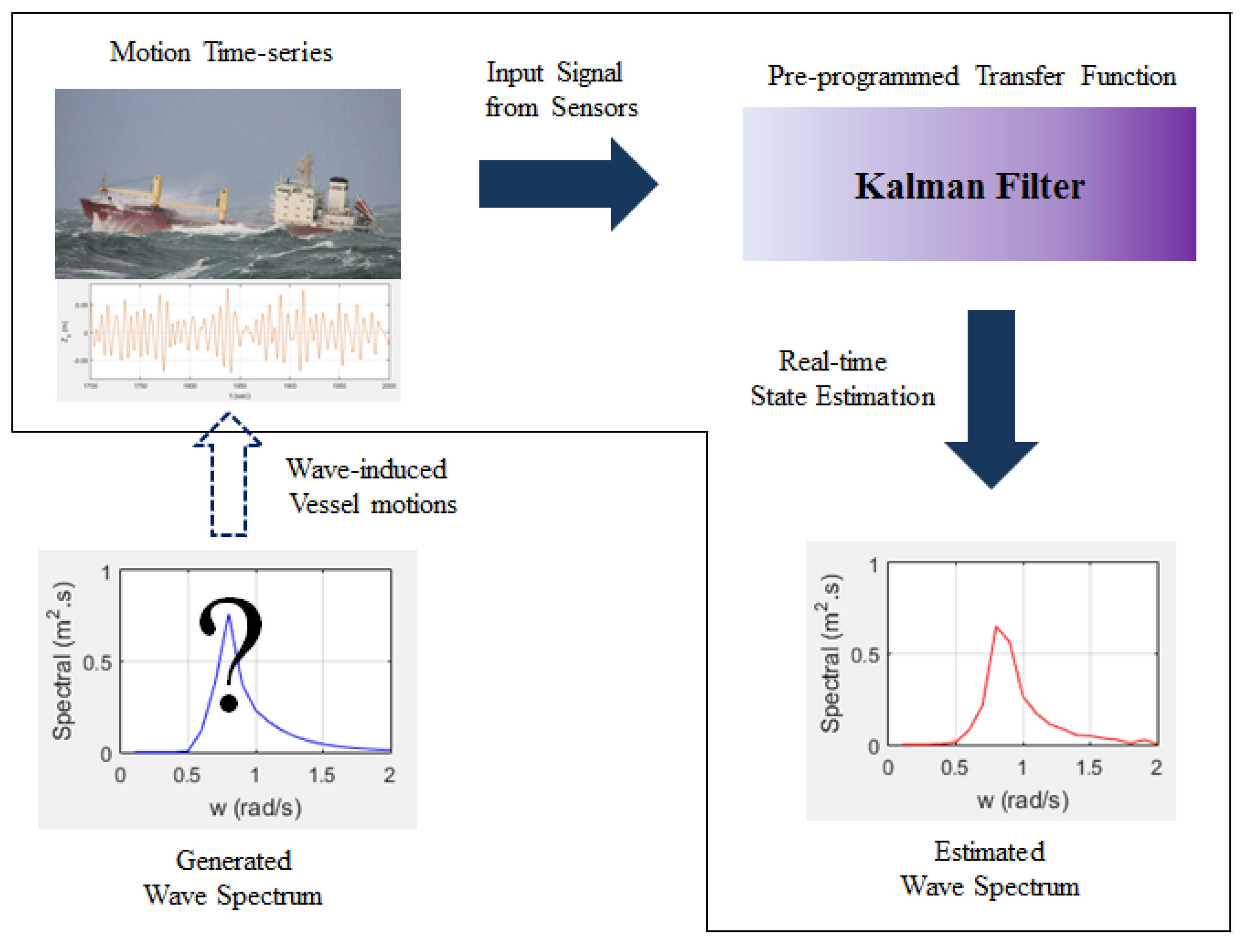
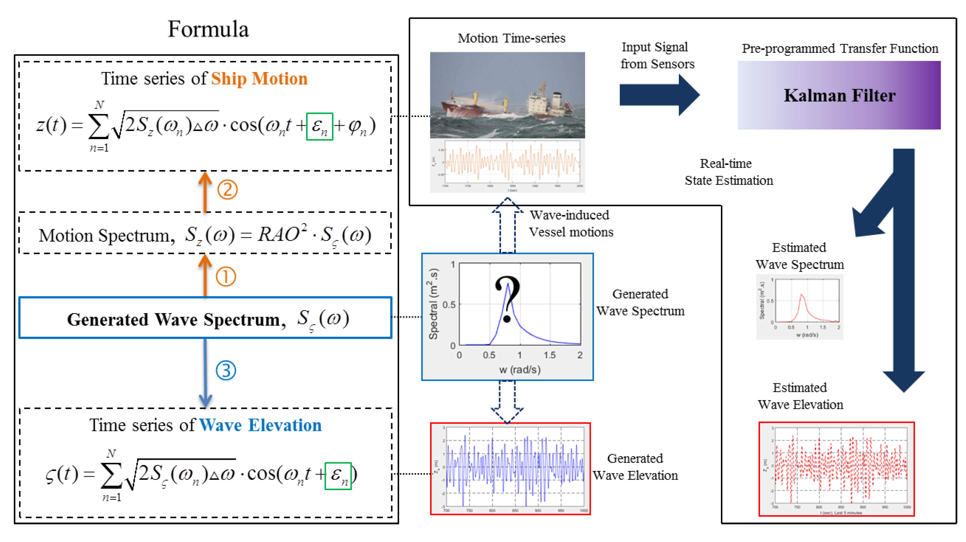
The research using the Kalman filter for the inverse estimation of ocean waves is very rare until recently despite the powerful advantages of the Kalman filter. Two papers [7,8] are representative. The Kalman filter in [8] was applied to ocean wave estimation while using synthesized motion data. In [7], the motion data of the actual field from a real ship was used. Nevertheless, this research is still in the development phase and it needs to be elaborated [9]. Figure 1 demonstrates the overall process of the wave spectrum estimation process while using the Kalman filter.

The Kalman filter is difficult to estimate high-frequency waves where the vessel’s response is weak. Thus, in the case of large vessels, additional high-accuracy sensors may be utilized or other responses sensitive to high frequencies may be used. More research is needed on this issue and the Kalman filter setting alone may be the solution [7].

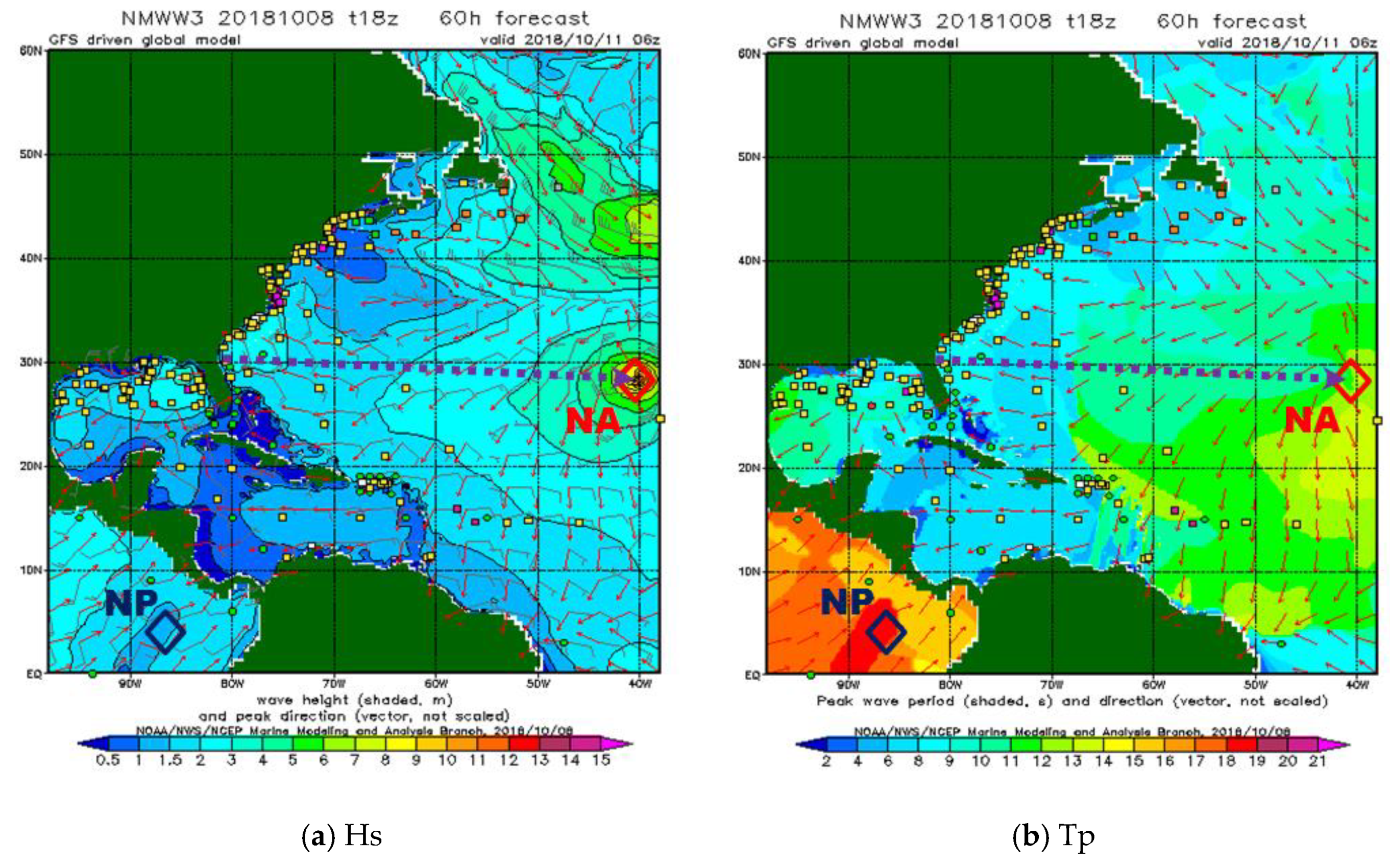
Figure 2 shows the actual sea conditions at North West Atlantic. They represent significant wave height, Hs (a) and spectral peak period, Tp (b) at the same time, respectively. It can be seen that high-frequency waves with a Tp less than 5 s (or $\omega$ > 1.257 rad/s) occupy a large portion in the figure. Therefore, estimating those wide-spreading high-frequency waves is of importance. Accordingly, it is important to design the Kalman filter, so that the high-frequency waves can also be estimated in a robust manner.

In [8], the frequency range was limited up to 1.15 rad/s since higher frequencies can cause problems when using Kalman filter. However, in this paper, the estimation range was extended to 2.0 rad/s, so that those high-frequency waves can be recovered. The cause of overestimation at the high-frequency zone and its remedy are investigated and new algorithms that suppress those overestimations are proposed. The numerical test results are promising for various wave conditions, vessel types, and sensor errors. Moreover, the present Kalman filter technique applied to the inverse problem successfully reproduces, not only the real-time wave spectrum, but also the real-time wave elevation. In this paper, ‘wave elevation’ means the time series of irregular wave profile. The estimation of wave elevation is very important for the active control in many ocean-engineering applications. As far as the authors know, the real-time inverse estimation of wave elevation by the Kalman filter cannot be found in the open literature.

The developed technology is relatively inexpensive and it has an advantage that the wave can be continuously estimated along a ship’s passage. According to recent statistics, the number of merchant ships sailing around the world in 2017 is about 50,000 [11] i.e., there are already 50,000 potential sensors on those vessels over the world, which means that a continuous build-up of big real-time ocean wave data through the inverse algorithm is possible with a robust network among ships.

2. Formulation for Modeling

2.1. Conventional Kalman Filter

The Kalman filter is an algorithm that estimates the state based on the statistical properties with the measurement while using sensors. The sensor contains sensor errors and the modeled governing equation does not perfectly match the system. Kalman filtering is applied to the system model of Equations (1) and (2) in the state space. It assumes that there exists a model error $w$ in the state $x$ and a sensor error $v$ in the measurement z during the transition to the next time step.

$$x_{k+1}={\varphi }_k{x}_k+w_k$$

(1)

$$z_k=H_k{x}_k+v_k$$

(2)

where

$\begin{array}{l}{x}_k=\mathrm{process}\mathrm{state}\mathrm{vector}\\ {\varphi }_k=\mathrm{state}\mathrm{transition}\mathrm{matrix}\\ w_k=\mathrm{model}\mathrm{error}\mathrm{vector}\\ z_k=\mathrm{measurement}\mathrm{vector}\\ H_k=\mathrm{output}\mathrm{matrix}\\ v_k=\mathrm{sensor}\mathrm{error}\mathrm{vector}\end{array}$

The covariance for each of the two errors is given by;

$$Q=E[w_k{w}_k^T]$$

(3)

$$R=E[v_k{v}_k^T]$$

(4)

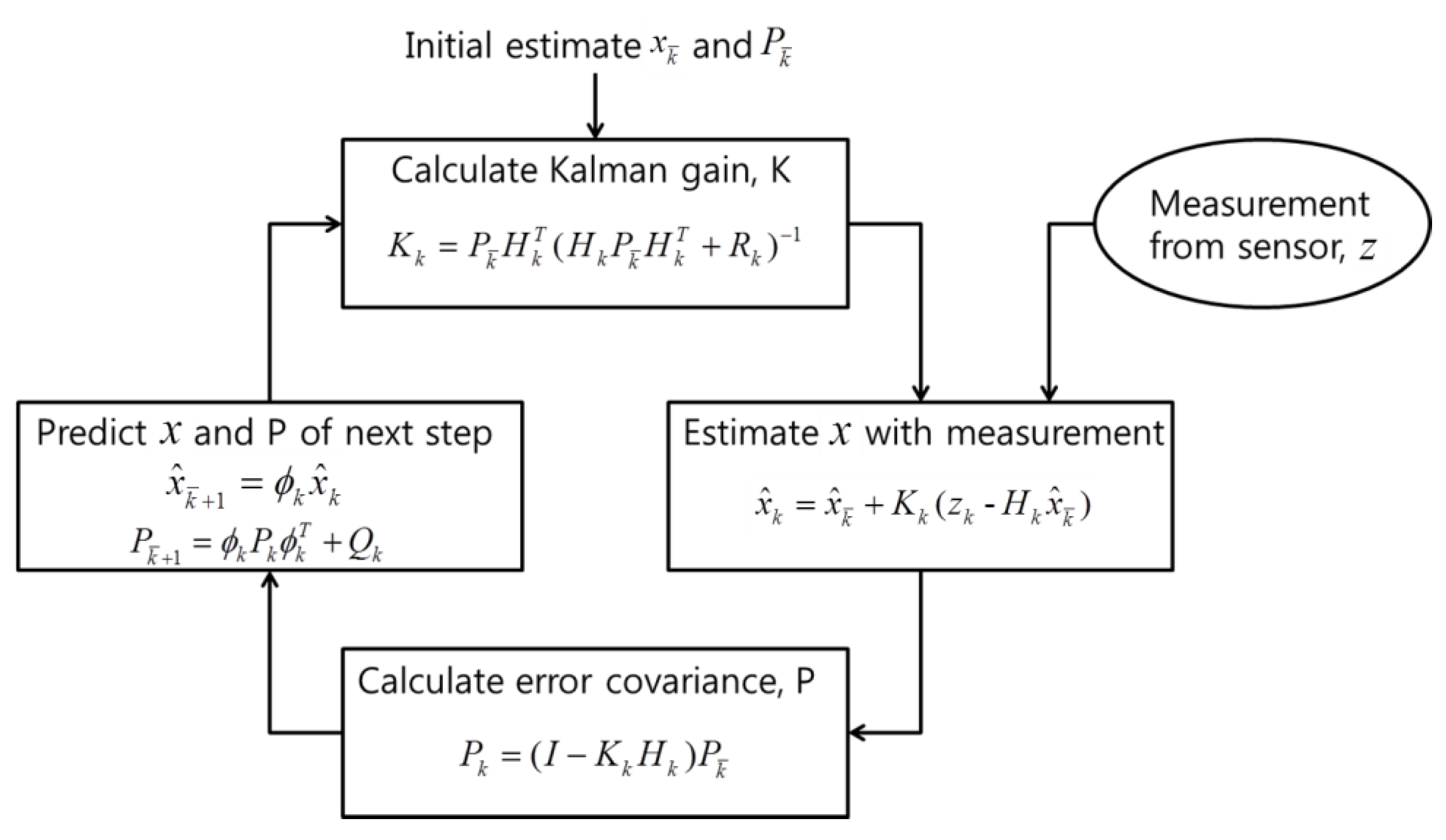
The Kalman filter keeps reducing the prediction error of the state x through the recursive calculating process. The process is made up of four steps, as described in Figure 3. The superscript ‘-’ means a predicted value for the next time step. Otherwise, it means a calculated (or estimated) value from measurement at the current step.

$\begin{array}{l}\mathrm{where},\\ x_{\overline{k}}=\mathrm{predicted}\mathrm{state}\mathrm{vector}\\ x_k=\mathrm{estimated}\mathrm{state}\mathrm{vector}\\ P_{\overline{k}}=\mathrm{predicted}\mathrm{error}\mathrm{covariance}\mathrm{matrix}\\ P_k=\mathrm{estimated}\mathrm{error}\mathrm{covariance}\mathrm{matrix}\\ K_k=\mathrm{Kalman}\mathrm{gain}\\ Q_k=\mathrm{model}\mathrm{error}\mathrm{covariance}\mathrm{matrix}\\ R_k=\mathrm{measurement}\left(\mathrm{sensor}\right)\mathrm{error}\mathrm{covariance}\mathrm{matrix}\end{array}$

The initial state $x_{\overline{1}}$ is to be estimated and the initial error covariance, $P_{\overline{1}}$ should be determined by the designer. If initial P ($P_{\overline{1}}$) is too small, then it will result in small Kalman gain, K by Equation (5) in the beginning of calculation. A small K means giving more weight to sensor measurement than prediction. Subsequently, at the beginning of the filtering, the measurement is relatively neglected and the prediction is overly counted. In other words, the $P_{\overline{1}}$ determines the initial convergence rate of the state x. Small P delays the initial convergence rate. Therefore, when the designer does not have prior knowledge of x, reasonably large initial error covariance, $P_{\overline{1}}$ should be set [13].

R is measurement error covariance that is generally determined from the error performance of the given sensor. An adaptive R may be applied when the sensor error is not statistically constant in the actual filtering process. H is the matrix that defines the relationship between state, x and measurement, z. In the estimation step, optimum x is calculated by using the weight factor, K in the Equation (6).

$$K_k=P_{\overline{k}}{H}_k^T{(H_k{P}_{\overline{k}}{H}_k^T+R_k)}^{-1}$$

(5)

$${\widehat{x}}_k={\widehat{x}}_{\overline{k}}+K_k^{}(z_k-H_k^{}{\widehat{x}}_{\overline{k}})$$

(6)

$$P_k=(I-K_k^{}{H}_k^{})P_{\overline{k}}$$

(7)

In the prediction step, P is increased by model error covariance, Q. Q is a design parameter that can be adjusted by the designer. This process is repeated:

$${\widehat{x}}_{\overline{k}+1}={\varphi }_k{\widehat{x}}_k$$

(8)

$$P_{\overline{k}+1}={\varphi }_k{P}_k{\varphi }_k^T+Q_k$$

(9)

The conventional Kalman filter is not directly suitable for practical applications. Therefore, the research that is related to using Kalman filter mainly focuses on the design of an adaptive type to fit a specific model, including the optimization of the design factors, R and Q. The optimized Q and R lead to the improvement of estimation performance of the filter. In the following, we explain how the algorithm can be utilized for the real-time inverse estimation of ocean wave spectra and elevation from vessel-motion sensors.

2.2. Main Formulas for Inverse Wave Estimation

References [7,8] presented the essential formulas, including the output matrix as Equation (11) i.e., the use of vessel’s hydrodynamics for wave spectrum estimation by utilizing the Kalman filter. Equations (1) and (2) are used as the system model equations. The state transitional matrix ${\varphi }_k$ is identity and $X$ is the complex wave amplitude in this case.

As in Equation (10), this model has an important premise. It assumes that the measured vessel motion is the result of incoming waves that were weighted by a transfer function [7]. The vessel’s transfer functions are complex, which means that they have amplitude and phase. The amplitude of transfer function is called response amplitude operator (RAO).

$$z(t)\cong \mathrm{Re}({\displaystyle \sum }_{j=1}^{n_f}T{F}_j\times (x_{2j-1}+i{x}_{2j})(\cos ({\omega }_{j}t)+i\sin ({\omega }_{j}t)))$$

(10)

where

• z: vessel motion
• $x_{2j-1}$: real part of complex wave amplitude
• $x_{2j}$: imaginary part of complex wave amplitude
• $\omega$: intrinsic frequency of harmonic
• $n_f$: number of harmonics to estimate
• $T{F}_j$: complex-valued transfer function for frequency j

The matrix type of $H$ becomes

$$H_{jkl}={\left[\begin{array}{l}\mathrm{Re}(T{F}_{jl})\cos ({\omega }_{j}k△t)-\mathrm{Im}(T{F}_{jl})\sin ({\omega }_{j}k△t)\\ -\mathrm{Im}(T{F}_{jl})\cos ({\omega }_{j}k△t)-\mathrm{Re}(T{F}_{jl})\sin ({\omega }_{j}k△t)\end{array}\right]}^{\prime }$$

(11)

where

• j: jth frequency
• k: kth time instant
• l: lth response
• $H_{jkl}$: output matrix
• $△t$: time step interval

In [8], the conventional Equations (5), (6), and (9) were used for prediction and estimation. However, in the prediction of x, Equation (13) was used instead of Equation (8) i.e., the average value for three-time instants is applied as the state prediction value, ${\widehat{x}}_{\overline{k}+1}$. In addition, P was computed by Equation (12) instead of Equation (7). Equation (12) was used for stability reasons and it is called the ‘Joseph Form’ [14]. In fact, Equation (7) is derived from Equation (12). Accordingly, either can be used to calculate P.

$$P_k=(I-K_k^{}{H}_k^{})P_{\overline{k}}{(I-K_k^{}{H}_k^{})}^{\prime }+KR{K}^{\prime }$$

(12)

$${\widehat{x}}_{\overline{k}+1}=1/3\cdot ({\widehat{x}}_k+{\widehat{x}}_{k-1}+{\widehat{x}}_{k-2})$$

(13)

According to [8], the adaptive approach has been considered, because it cannot be assured that the process is completely known and that the steady state is reached due to the change of sea condition and ship’s heading. Equation (14) is the Adaptive R equation. The ‘diag’ means taking the diagonal from a matrix into a vector form and vice-versa.

$$R=dia{g}^2(E[z_k-H_k^{}{\widehat{x}}_{\overline{k}},{(z_k-H_k^{}{\widehat{x}}_{\overline{k}})}^{\prime }])+H_k{P}_{\overline{k}}{H}_k{}^{\prime }$$

(14)

The initial value of the state is as follows:

$${\widehat{x}}_{\overline{1}}=0$$

(15)

In the present paper, the above Equations (1), (2), (5)–(11), and (15) are applied. The rest of the equations and other conditions are set to suit the vessel that is considered and computer specifications.

Using the state, x, which is an estimated value from the filter, the wave spectrum and wave elevation can be calculated from the following equations. The reconstruction of both wave spectra and wave elevation is possible since the state variable x and motion transfer function TF are complex variables:

$$S_{\varsigma }({\omega }_i)=0.5\times \frac{1}{\mathsf{\Delta }{\omega }_i}\times ({\widehat{x}}_{2i-1}^2+{\widehat{x}}_{2i}^2)$$

(16)

$$\varsigma (t)=[\cos ({\omega }_1\cdot t),-\sin ({\omega }_1\cdot t)\dots \cos ({\omega }_n\cdot t),-\sin ({\omega }_n\cdot t)]{[{\widehat{x}}^{}{}_1{\widehat{x}}^{}{}_2\dots {\widehat{x}}^{}{}_{2n-1}{\widehat{x}}^{}{}_{2n}]}^{\prime }$$

(17)

where

• $S_{\varsigma }(\omega )$: wave spectrum
• $\mathsf{\Delta }\omega$: frequency interval
• $\varsigma$: wave elevation

Regarding the determination of R and Q values, R can be determined based on the real sensor’s performance before or while operating the filter. Thus, it is practical to specify R. On the other hand, Q is generally more difficult to determine, because Q is sometimes dynamically varying during filtering and it cannot be directly observed in the process of estimation. In a simple process, satisfactory estimation can sometimes be obtained by setting the appropriate Q. The tuning of Q and R can provide excellent filter performance, regardless of whether there is a reasonable basis for choosing the parameters [15]. Thus, [16] described R and Q as model-specific “tuning knobs” that determine filter performance and expressed choosing them as “spirit of observer design”.

First, $P_{\overline{1}}$ was set large enough to make the initial convergence fast, as Equation (18). This is because the initial state is uncertain. In the long run, this initial value does not make much difference in the filter performance [13]. Subsequently, to design the proper fixed value of Q, it is assumed that there is no measurement error, which means that R is 0. From a number of tests, the appropriate Q value was set as Equation (19), so that the estimation is good enough and P does not diverge.

$$P_{\overline{1}}=\left[\begin{array}{cc}{50}_{i\times i}& 0\\ 0& {50}_{i\times i}\end{array}\right]$$

(18)

$$Q=\left[{\begin{array}{cc}{10}^{-5}{}_{i\times i}& 0\\ 0& {10}^{-5}\end{array}}_{i\times i}\right]$$

(19)

where

• i: half the length of x

Only heave motion is considered to simplify the case. R was calculated by Equation (20) and it remains as the fixed value while the filter is running. The standard deviation of heave motion sensor error is set to be 2.3 cm, referring to the test result of a commercial product [17]. Thus, when only heave is considered, R is $5.29\times {10}^{-4}$, which is the square of 0.023 m.

$$R_{}=diag\left(\begin{array}{l}{\sigma }_1{}^2\\ {\sigma }_2{}^2\\ ⋮\\ {\sigma }_{l-1}{}^2\\ {\sigma }_l{}^2\end{array}\right)$$

(20)

where

• $\sigma$: sensor noise (error) standard deviation
• l: lth response or mode

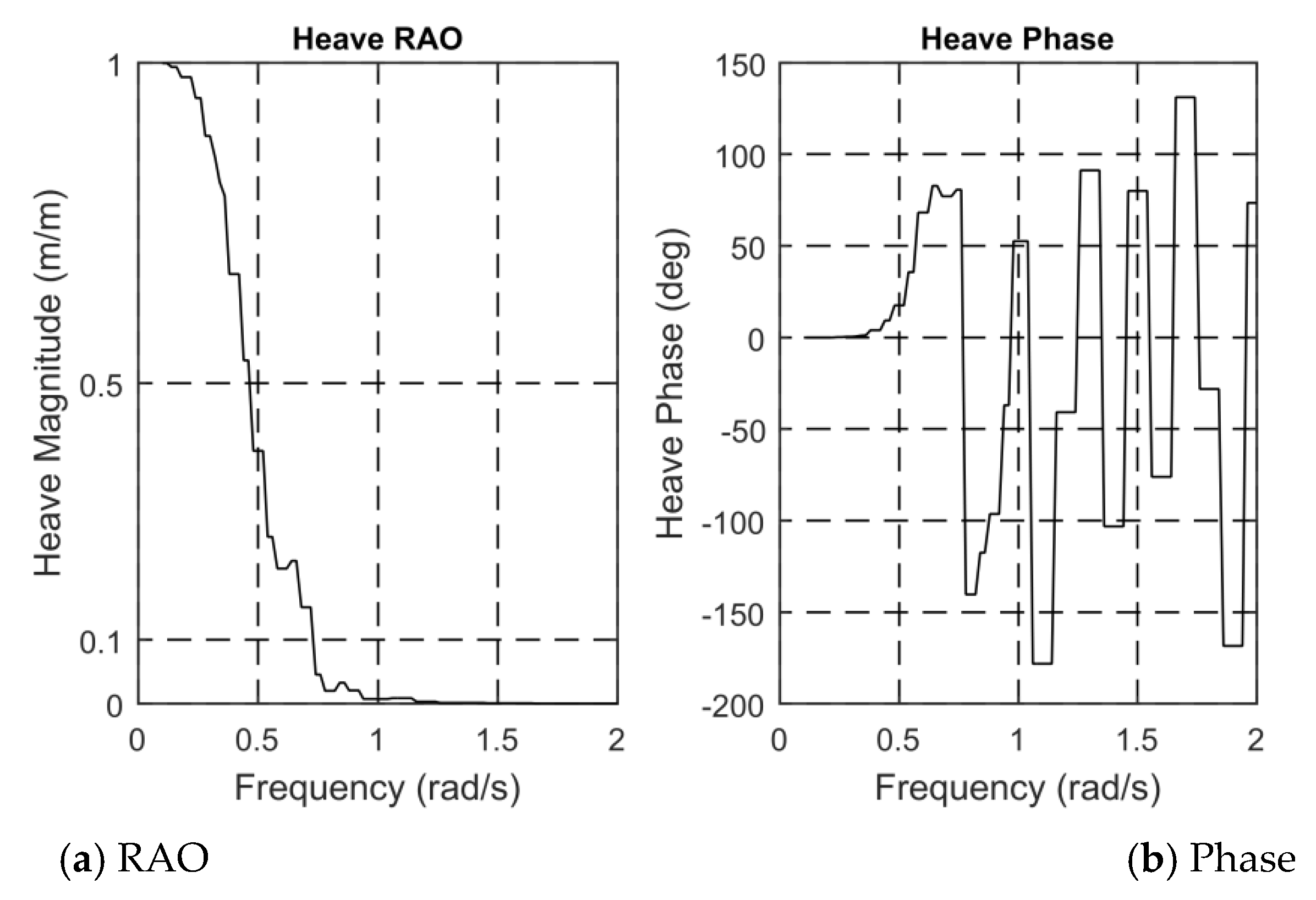
A freely floating FPSO (Floating Production Storage and Offloading) in Figure 4 was selected as the vessel. The total number of 1831 quadrilateral panels was used after the convergence test. The details of the vessel are given in [18]. Figure 5 is the RAO of the FPSO. The vessel’s transfer function (or RAO) was numerically computed while using a three-dimensional (3D) diffraction/radiation panel program, WAMIT software.

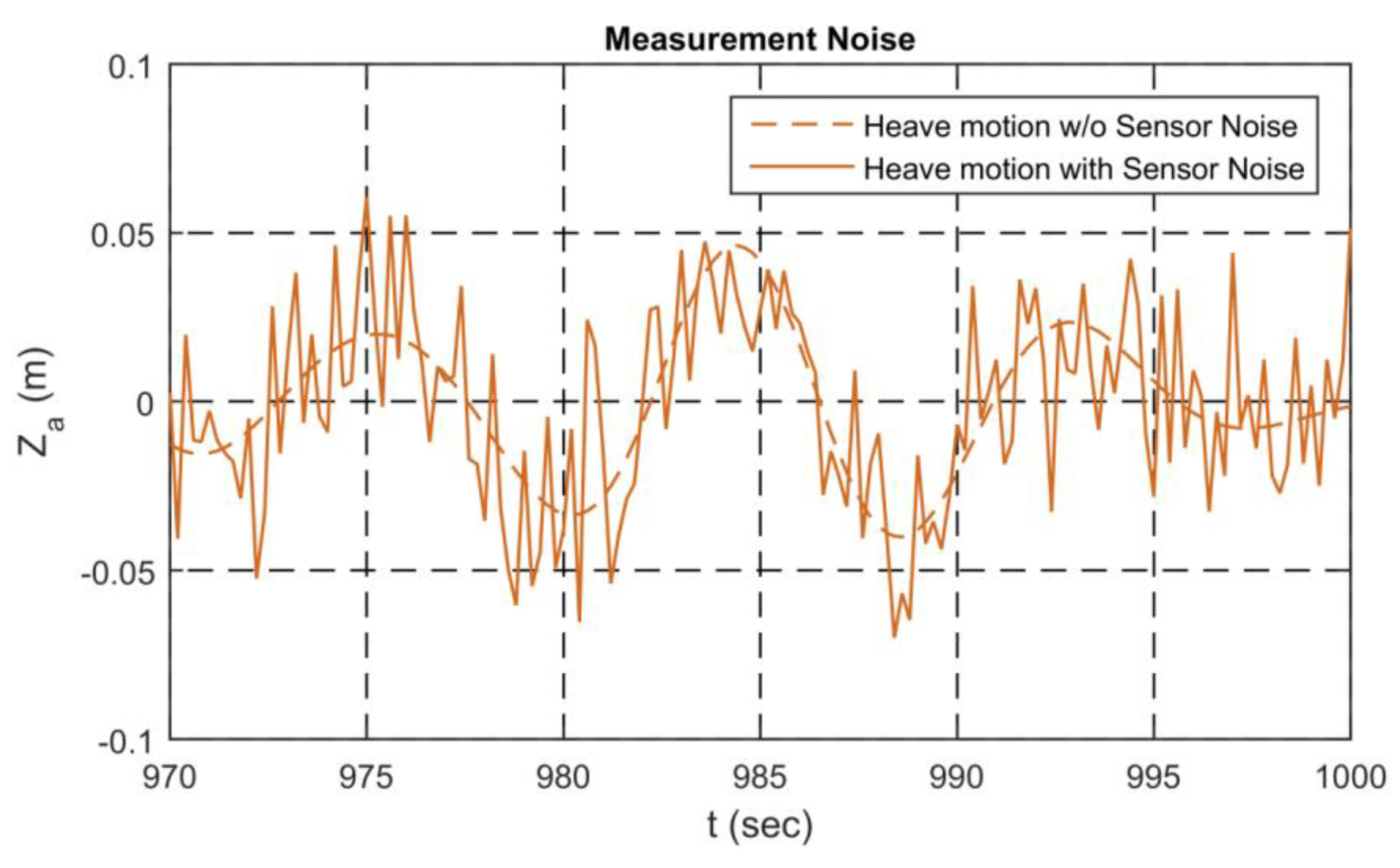
A uni-directional JONSWAP wave spectrum with Hs = 2 m, Tp = 7 s, and enhancement parameter = 2.2 is considered. The significant wave height, Hs is defined as the average of the 1/3 largest waves. It can be calculated from either wave spectrum or wave time series. Tp is the spectral peak period. Hs and Tp are used as key index parameters since the purpose of the Kalman filtering is to inversely estimate the overall shape of the spectrum. Subsequently, the corresponding heave motion spectrum was calculated while using the calculated RAO. Afterwards, the corresponding irregular-motion time series were generated by Equation (29). Subsequently, a white noise that was equivalent to the standard deviation of sensor error 2.3 cm was artificially added (Figure 6). Afterwards, the motion-time-series data, including the sensor error, was inputted to the present Kalman filter process. The frequency range of the white noise is set to be the same as that of input wave spectrum.

The previous equations and conditions were applied. First, the frequency range was limited to 0.1~1.15 rad/s, as in [8]. The Kalman filter was run for 1000 s. The real-time spectra were calculated during that time. The spectral estimation was good after the initial transient stage, as indicated in Figure 7. This shows that the Kalman filter is well designed up to this point. However, we found some problem when the frequency range is extended to higher-frequency regions, as shown in the next example.

2.3. Design of Modified TF to Suppress Overestimation in High-Frequencies

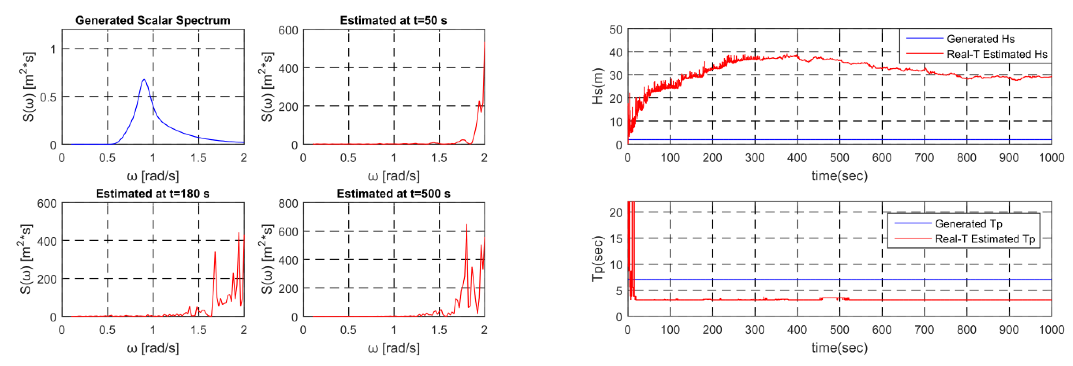
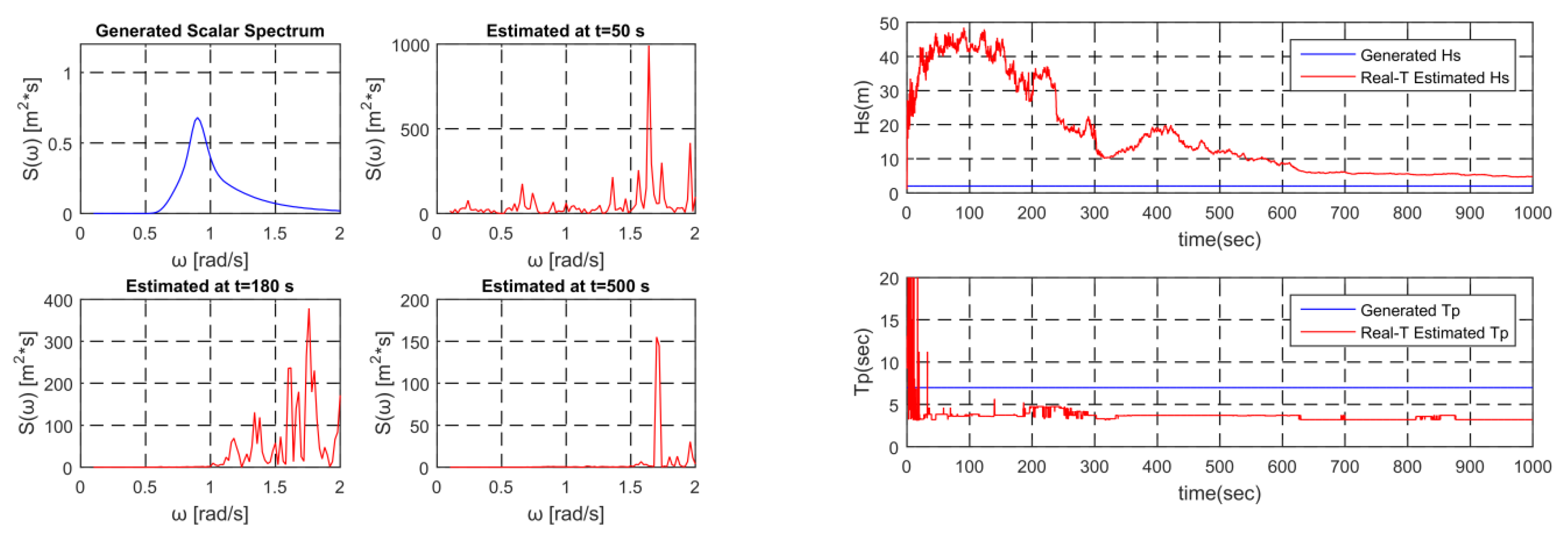
The performance of the designed Kalman filter was examined when the frequency range is extended to 2.0 rad/s. In Figure 8, we start to see some problem i.e., excessive estimation of spectral amplitude in the high frequency region.

No overestimation occurred when the sensor error was removed. In case there is sensor error and RAO is intentionally amplified, so that its magnitude is more than 1 in all frequency region, overestimation did not occur. Therefore, it is expected that the cause of the overestimation at the high frequency region is the combination of sensor errors and small values of RAO. In order to better understand the phenomenon, the internal variables, P and K for every frequency component during the operation of the filter were analyzed.

Figure 9 shows a comparison of the changes of the internal variables P and the absolute value of K in the frequency domain during the Kalman filter operation for both cases i.e., (a) and (b) when the maximum frequency is 1.15 rad/s and (c) and (d) when the maximum frequency is changed to 2.0 rad/s. In the case of (a) and (b), the P and K values converge to proper values after initial transient stage. However, in the case of (c) and (d), the P and K values do not converge well and the errors in the high frequency region are particularly large. The convergence rates in the high frequency region are also very slow. This is due to Equation (7) of the ‘Calculate P’ step in the Kalman filter loop. P is decreasing each time step by the equation. The high-frequency region of $(I-K_k^{}{H}_k^{})$ is close to 1, the element of an identity matrix, since the H is small in the high-frequency zone due to the motion characteristics (RAO) of the vessel. Therefore, the high-frequency region of P, which is multiplied by $(I-K_k^{}{H}_k^{})$ every time step, slowly decreases.

P is a variable that determines K in Equation (5) of the ‘Calculate K’ step. The slow decreasing of P also slows down the convergence rate of K. Therefore, in Figure 9d, the convergence speed of K also becomes slow. K is gain between the measured value and the predicted value in Equation (6) of ‘Estimate x with measurement’ step. The overestimated K in the high frequency range gives an excessive value of x, which is the estimated result. Essentially, the small response in the high frequency region of RAO with respect to the given sensor error causes an overestimation problem.

First, as a potential solution to overcome the phenomenon of overestimation in the high frequency region, while using multi-motion signals was attempted i.e., Surge, Sway, Roll, Pitch, and Yaw were added so that a total of six motions can be used. It may be possible that the ill behavior of heave in the high frequency region can be compensated by sensor fusion. The test results (Figure 10) show that the unfavorable behavior is improved when compared to the heave only case, but overestimation still occurs i.e., the generalization of Kalman filter technique to include all 6DOF motions helps the problem, but is not highly effective.

Meanwhile, the phenomenon of excessively amplified noise is mentioned as a problem of the inverse filter that is used in the image restoration field [19]. This problem can occur when the transfer function is zero or very small. If the measured signal has sensor error, it is more amplified at high frequencies. In the image restoration, the Wiener filter is used to solve this problem. In this regard, we applied the principle of the Wiener filter to the present the Kalman-filter technique, as described in the following.

Reference [20] explains some filters for original-image-restoration from blurred images. First, the Inverse filter is introduced. Assuming that the blurring function D, which is a sort of transfer function, is known, the inverse filter can be directly used in the frequency domain to recover the original image. The observation equation can be expressed in the frequency domain, as;

$$\mathrm{G}\left(\mathrm{u},\mathrm{v}\right)=\mathrm{F}\left(\mathrm{u},\mathrm{v}\right)\mathrm{D}\left(\mathrm{u},\mathrm{v}\right)$$

(21)

where

• G: observed image
• F: original image
• D: blurring function

The original image F(u,v) can be restored by filtering the observation G(u,v). The inverse filter $\frac{1}{\mathrm{D}\left(\mathrm{u},\mathrm{v}\right)}$ provides a perfect estimate of the original image in the case of no noise as follows:

$$\widehat{\mathrm{F}}=\mathrm{G}\left(\mathrm{u},\mathrm{v}\right)\frac{1}{\mathrm{D}\left(\mathrm{u},\mathrm{v}\right)}$$

(22)

where

• $\widehat{\mathrm{F}}$: estimated image

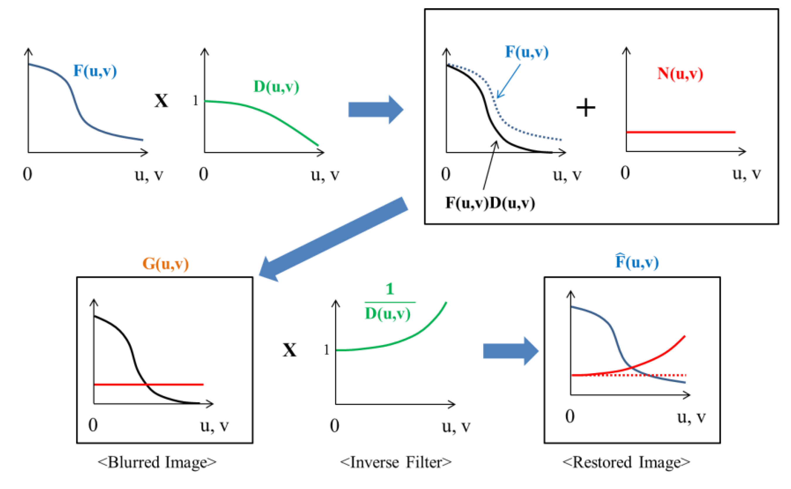
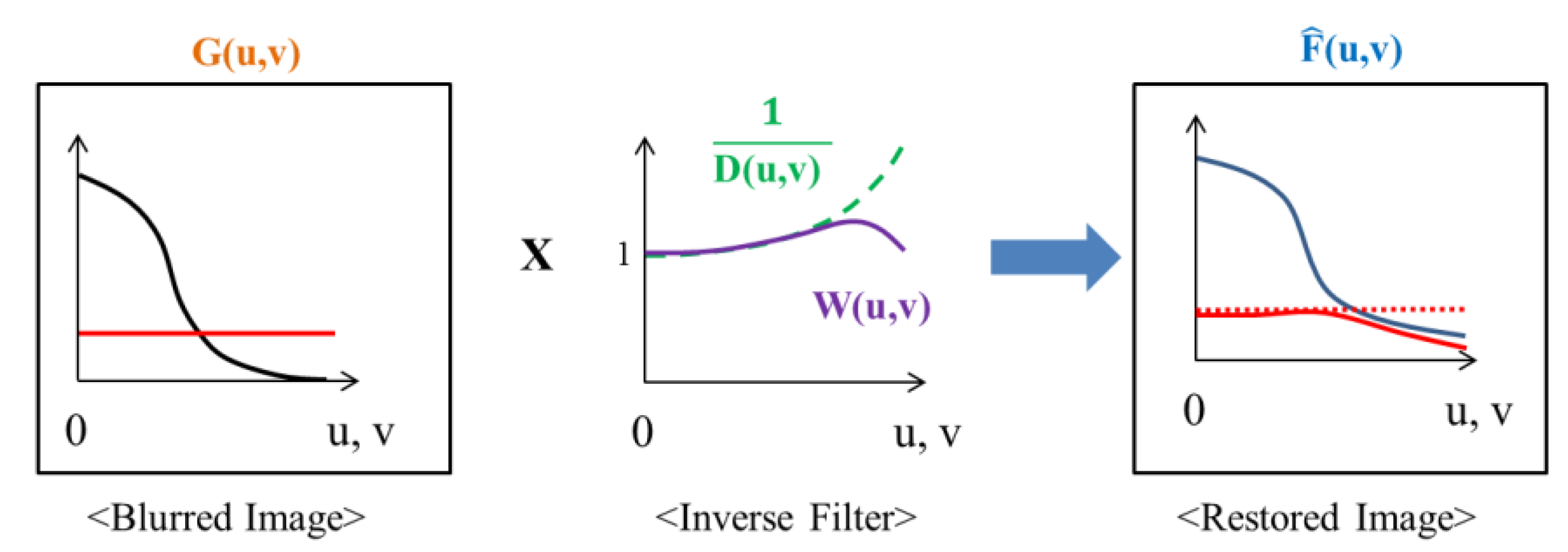
However, if there is sensor noise N(u,v) as Equation (23), the result will be filtered noise i.e., the sond term in Equation (24) and the desired image. The term is called “Inverse Filtered Noise” [20]. The inverse filter typically has very high gain at certain frequencies, where D(u,v) is small. The amplified noise at those frequencies will dominate the result. Figure 11 is the schematic diagram of noise amplification. In the bottom right of the figure, $\widehat{\mathrm{F}}$ the estimated image is amplified (red solid line) in the high frequency region by the inverse filter.

$$\mathrm{G}\left(\mathrm{u},\mathrm{v}\right)=\mathrm{F}\left(\mathrm{u},\mathrm{v}\right)\mathrm{D}\left(\mathrm{u},\mathrm{v}\right)+\mathrm{N}\left(\mathrm{u},\mathrm{v}\right)$$

(23)

$$\widehat{\mathrm{F}}=\mathrm{G}\left(\mathrm{u},\mathrm{v}\right)\frac{1}{\mathrm{D}\left(\mathrm{u},\mathrm{v}\right)}=\{\mathrm{F}\left(\mathrm{u},\mathrm{v}\right)\mathrm{D}\left(\mathrm{u},\mathrm{v}\right)+\mathrm{N}\left(\mathrm{u},\mathrm{v}\right)\}\frac{1}{\mathrm{D}\left(\mathrm{u},\mathrm{v}\right)}=\mathrm{F}\left(\mathrm{u},\mathrm{v}\right)+\frac{\mathrm{N}\left(\mathrm{u},\mathrm{v}\right)}{\mathrm{D}\left(\mathrm{u},\mathrm{v}\right)}$$

(24)

To overcome the noise sensitivity of the inverse filter, the Weiner filter can be used. It is defined in the frequency domain, as;

$$\begin{array}{l}\mathrm{W}(\mathrm{u},\mathrm{v})=\frac{{\mathrm{D}(\mathrm{u},\mathrm{v})}^{*}}{{(|\mathrm{D}(\mathrm{u},\mathrm{v})|}^2+\frac{{\mathrm{S}}_n(\mathrm{u},\mathrm{v})}{{\mathrm{S}}_f(\mathrm{u},\mathrm{v})})}{(\mathrm{When}\mathrm{S}}_n{(\mathrm{u},\mathrm{v})\mathrm{or}\mathrm{S}}_f(\mathrm{u},\mathrm{v})\mathrm{is}\mathrm{unknown},\frac{{\mathrm{S}}_n(\mathrm{u},\mathrm{v})}{{\mathrm{S}}_f(\mathrm{u},\mathrm{v})}\to \mathrm{C})\\ \end{array}$$

(25)

where

• ${\mathrm{D}(\mathrm{u},\mathrm{v})}^{*}$: complex conjugate of D(u, v)
• ${\mathrm{S}}_n(\mathrm{u},\mathrm{v})$: power spectrum of the noise
• ${\mathrm{S}}_f(\mathrm{u},\mathrm{v})$: power spectrum of the ideal image
• C: constant

In fact, the Wiener filter is used to minimize the mean square error between the estimated signal and the desired signal. It produces an estimate of the desired signal of a measured noisy signal, in principle, while assuming that original signal and noise are known [21]. However, it is common to use an approximation when the power spectra are not known. It means that the ratio ${\mathrm{S}}_n{(\mathrm{u},\mathrm{v})/\mathrm{S}}_f(\mathrm{u},\mathrm{v})$ can be substituted by a constant C. The C can be chosen by logistic trial and error [19,22] as Equation (25). In this paper, the original signal i.e., wave spectrum is assumed to be unknown. Accordingly, C can be determined by trial and error.

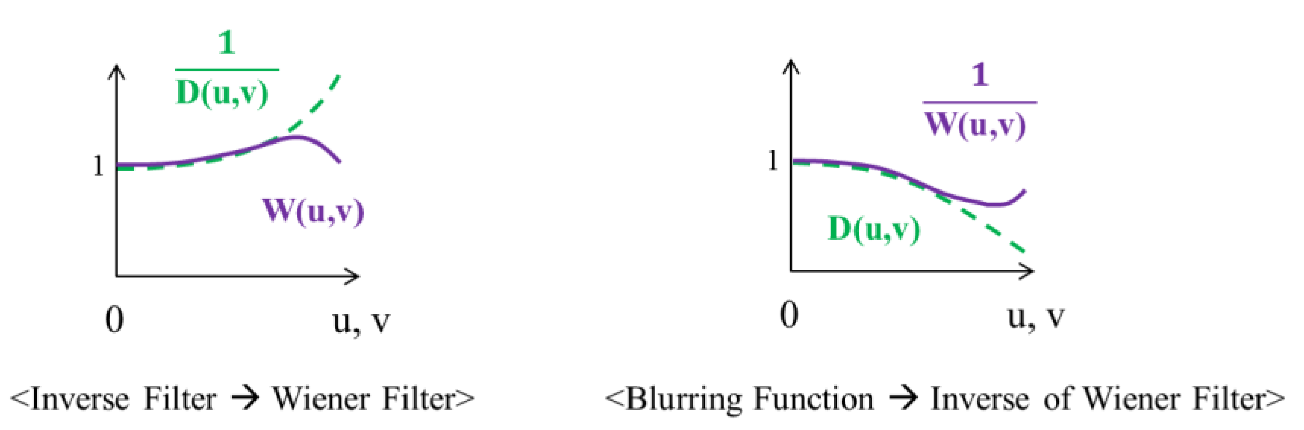
In Figure 12, through comparison with inverse filter (1/D), we see the effect of Wiener filter W(u, v). The Wiener filter suppresses the gain by a certain amount to suppress amplified noise in the frequency region where the magnitude of Inverse filter is too large. To see the effect of Wiener filter with respect to transfer function D, the inverses of both Inverse filter and Wiener filter are plotted in Figure 13; 1/W(u, v) increases the very small gain of D in the high-frequency region.

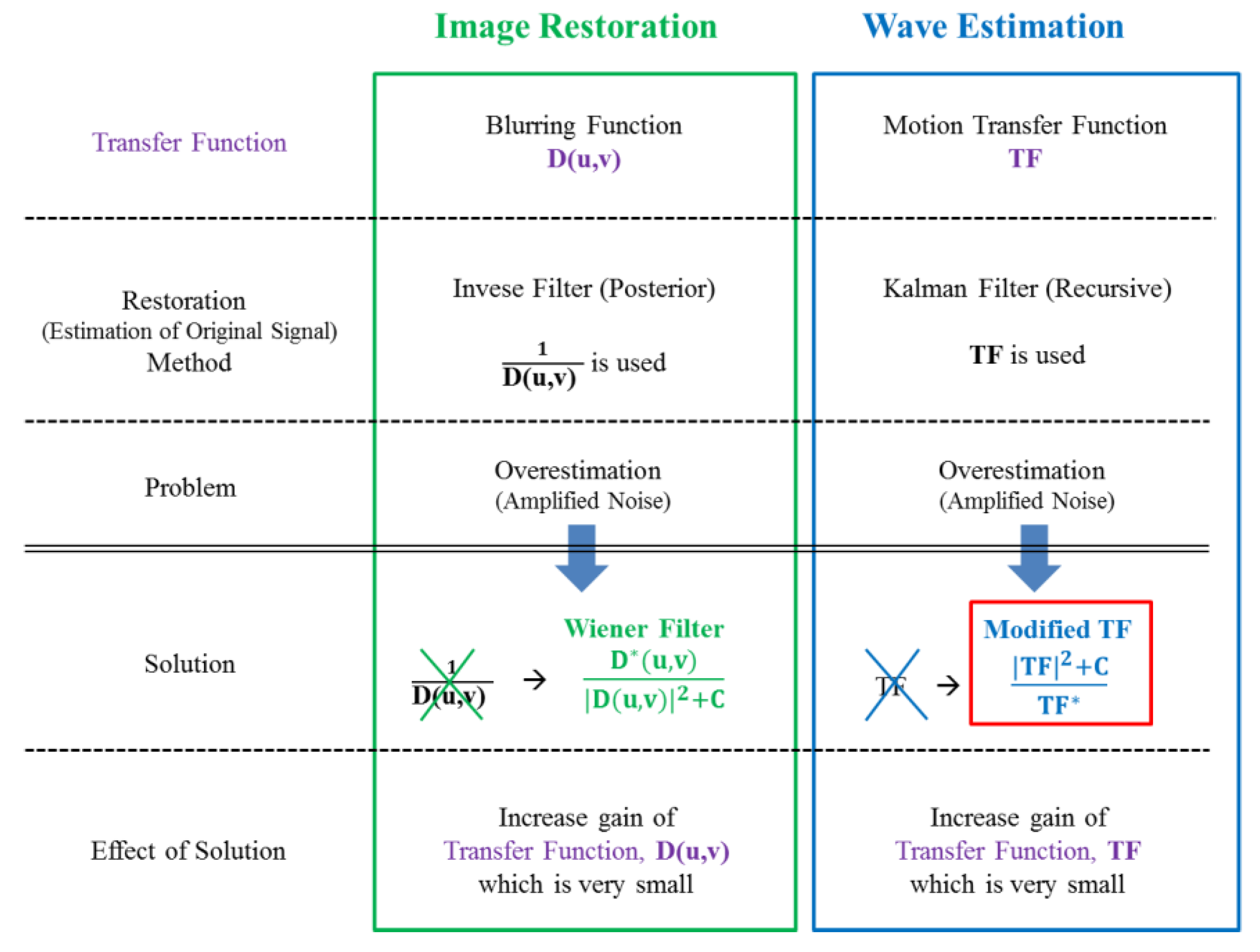
When comparing the wave estimation with the image restoration, F corresponds to wave, G to ship motion, and D to motion TF or H, respectively. Unlike the Inverse filter, the Kalman filter is the recursive filtering algorithm finding more accurate state with more measurements. However, at a particular time step, the Kalman filter also computes the original signal in the inverse direction from the measurement with sensor noise, while using the pre-programmed output equation between the state and measurement.

We applied the principle of Wiener filter to the present Kalman-filter technique for the inverse wave estimation in the frequency region where the magnitude of Inverse filter is too large. The issue is that the inverse form of transfer function like (1/D) cannot directly be applied to the Kalman filter. Rather, it is not in inverse form, but TF is included in H as equation (11). Therefore, we had to devise a way to modify the TF while keeping the Wiener’s effect the same. As mentioned earlier, the effect of the Wiener filter is to increase the gain of D by a certain amount in the frequency region where the magnitude is 0 or too small.

If Wiener filter W is used instead of Inverse filter (1/D) in Equation (24), noise term N/D is eliminated, and G $\times \mathrm{W}$ = F is established. Subsequently, G/F = 1/W. Let us put this as Equation (a). Meanwhile, in the Equation (6) in the Kalman filter, it is used as Z-HX. If we change these as variables of image restoration, it is G-DF. Assuming that there is noise, it is not 0 but G-DF = N. Afterwards, D = G/F-N/F and let us put this as Equation (b). When we input 1/W to D in the Equation (b), the Equation (b) becomes G/F = G/F−N/F by the Equation (a) and N/F becomes 0. That is, if we use 1/W instead of D in Kalman filter, we can obtain the effect of Wiener filter and eliminate the noise. In conclusion, the modified TF as Equation (26) was applied to the Kalman filter in the inverse form of Wiener filter. For easy comparison, Figure 14 is given.

$$\frac{(|\mathrm{TF}{|}^2+\mathrm{C})}{{\mathrm{TF}}^{*}}$$

(26)

where

• ${\mathrm{TF}}^{*}$: complex conjugate of TF

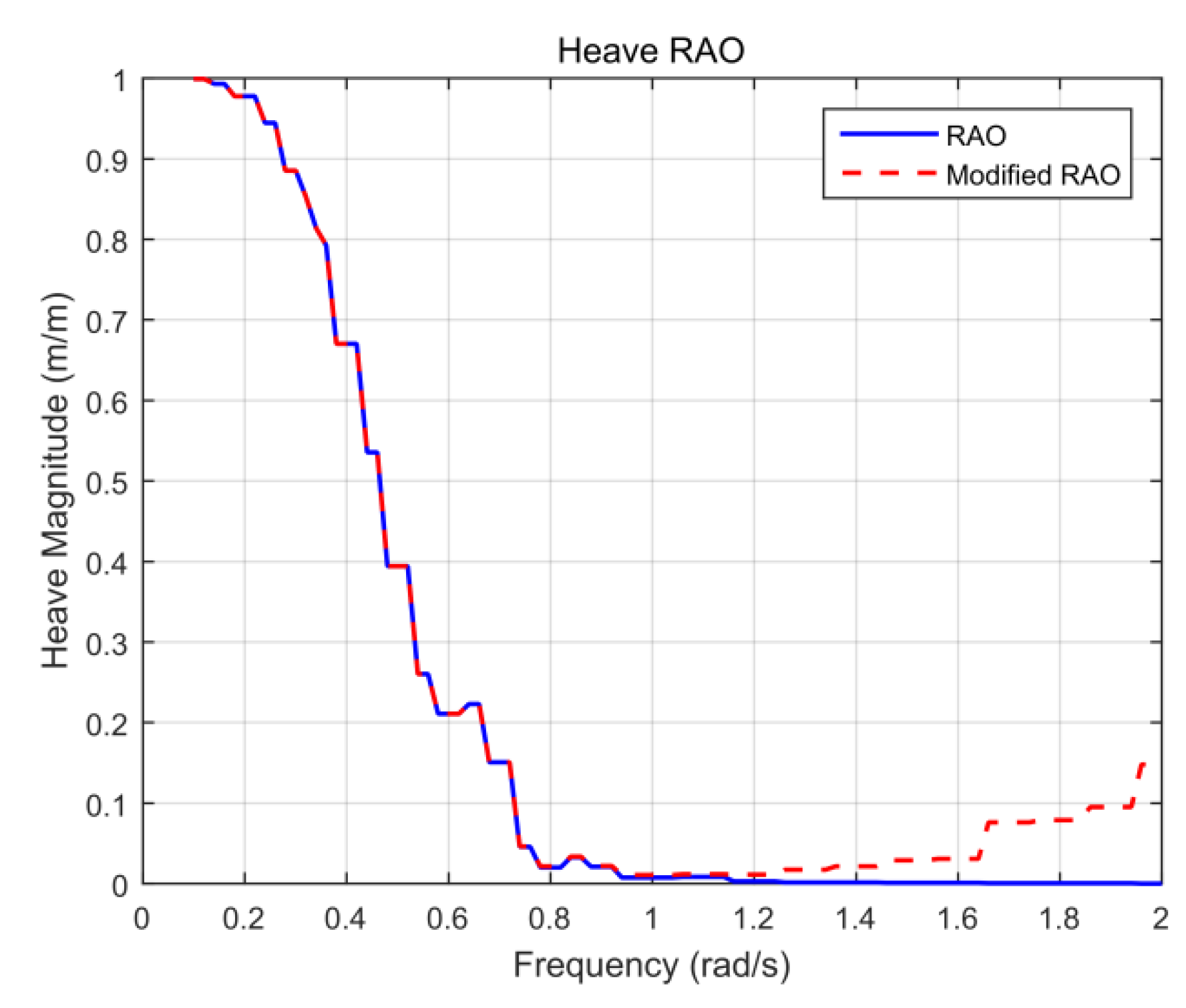
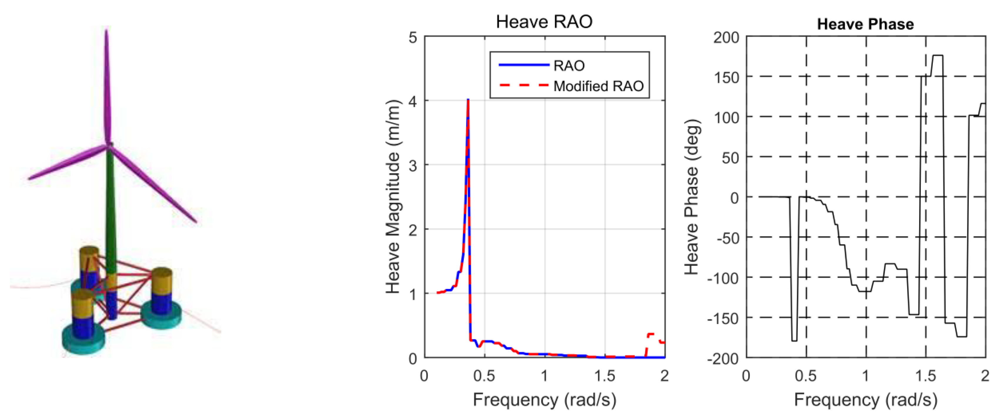
Through trials and errors, C was found to be 2.5 $\times {10}^{-5}$, when the sensor noise (error) standard deviation is 0.023 m. Figure 15 shows the Modified RAO (TF) when Equation (26) is applied. We aslo tested the formula for various wave conditions and two different floating platforms, such as FPSO and semi-submersible case, and the results are equally satisfactory. This is covered in detail in Section 3.2. The results show substantial improvement (overestimation does not occur) when the proposed modified motion TF is applied to the FPSO, as shown in Figure 16.

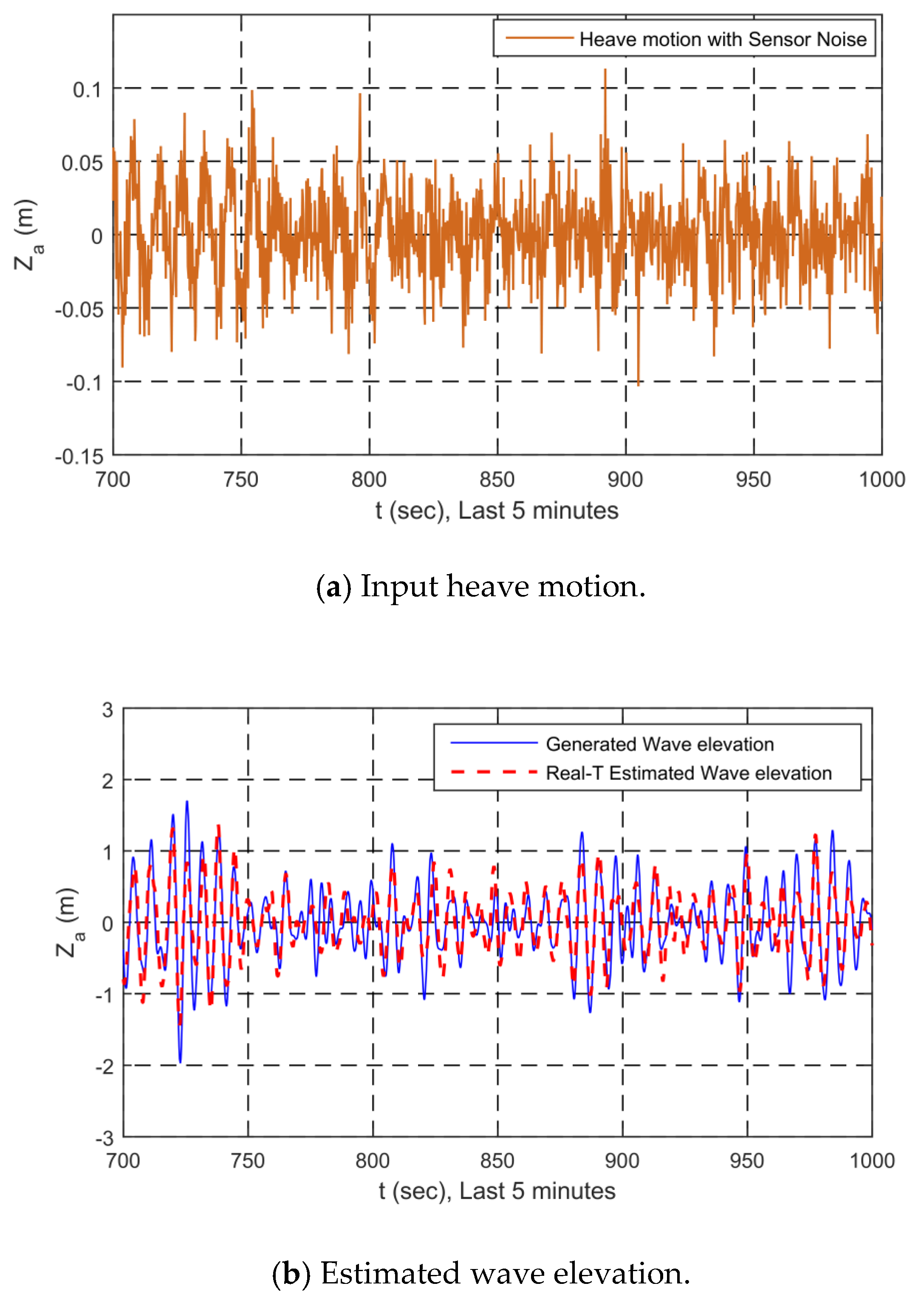
($x_{2j-1}+i{x}_{2j}$) is an incoming wave of a complex number in Equation (10). For the two states $x_{2j-1},{\mathrm{x}}_{2j}$ estimated by the Kalman filter, if Equation (17) is used, the real-time estimation of the corresponding wave elevation (actual wave profile) at each time is conducted (Figure 17) and Figure 18 shows the results. The real-time wave profile that was estimated by the Kalman filter is compared to the theoretically reconstructed wave profile by using the random phase and the relation between the wave and motion via the phase of transfer function.

Figure 17 describes the estimation process for wave elevation. In the case of the wave spectrum estimation, only the motion time series of the ship needs to be generated through the process of , ‚ in the figure. In the case of the wave elevation estimation, we need to additionally generate the original wave elevation through the ƒ calculation. This becomes the target for comparison with the estimated one. It should be noted that the motion and wave random pahses differ by the TF phase φ, so that the random phases of incident wave can be assigned.

In Figure 18, the original and inversely estimated wave profile agree very well. This means the the present Kalman filter technique applied to the inverse problem successfully reproduces not only the real-time wave spectrum, but also the real-time wave elevation. The latter is very important for the active control in many ocean-engineering applications. To the best knowledge of authors, the real-time inverse estimation of wave elevation by the Kalman filter cannot be found in the open literature. In [7,8,23,24], no time series of wave elevation was obtained although wave spectra were inversely estimated.

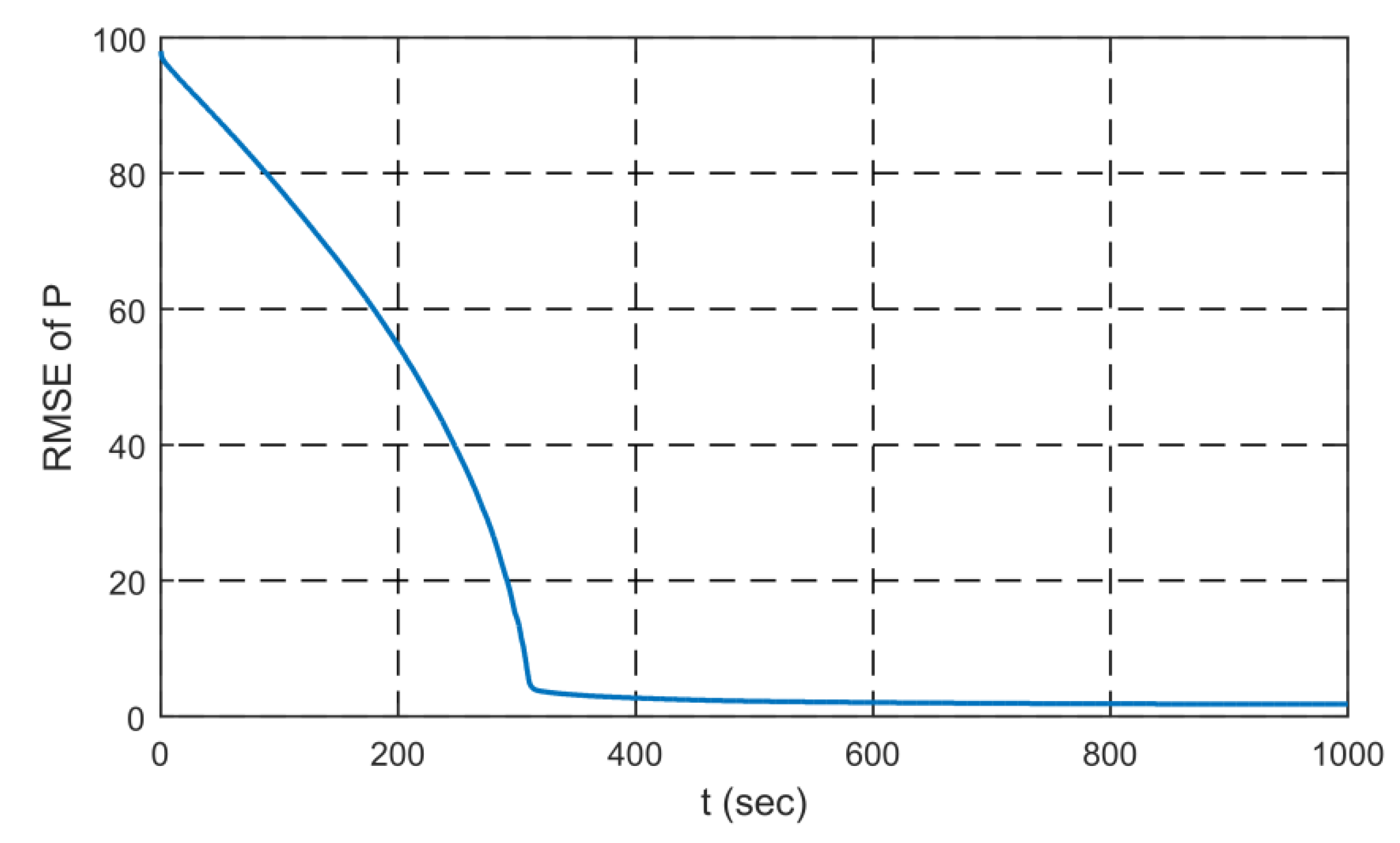
For further checking of convergence, RMSE of P is represented from Equation (27). The ‘trace’ means sum of diagonal elements. Figure 19 confirms that P does not diverge.

$$RMSEofP=\sqrt{trace(P)}$$

(27)

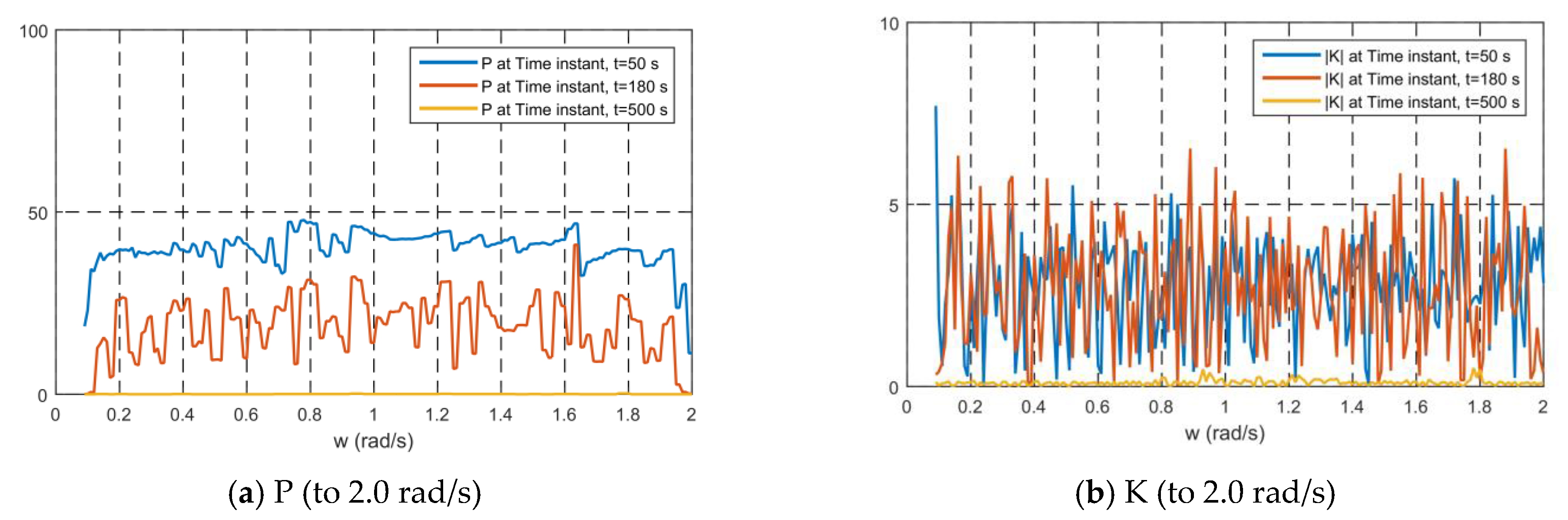
The variations of the internal variables P and K in the frequency domain were examined as well in Figure 20. When compared with the ‘~2.0 rad/s’ case of Figure 9c,d, it can be seen that both P and K converge near zero in the high frequency range at 500 s. The application of Modified TF suppresses K in the high frequency. Consequently, the overestimation of x does not occur in the high-frequency region when it is calculated by Equation (6).

The measurements from a sensor include sensor error. When the sensor maker provides sensor error information, we can set a reference value for R according to the information. However, a potential problem is that the statistical properties of sensor errors are not the same during actual measurements. Accordingly, [25] proposed an adaptive Kalman filter for harmonic signals. Therefore, to take advantage of the adaptive R, Equation (14), e.g., [8] is applied with the modified TF in subsequent tests. In the equation, only the diagonal component was taken from the covariance matrix for the errors. By two ‘diag’ processes, we can construct a diagonal matrix, so that it matches the dimensions of the $H_k{P}_{\overline{k}}{H}_k{}^{\prime }$ matrix.

To explain more about the dimensions of the $H_k{P}_{\overline{k}}{H}_k{}^{\prime }$ matrix, variable definition and dimensions are in

Table 1. Dimension of Variables.

Variable	Description	Dimension
x	State Vector	$n_x\times 1$
z	Measurement Vector	$n_z\times 1$
$\varphi$	State Transition Matrix	$n_x\times n_x$
H	Output Matrix	$n_z\times n_x$
P	Error Covariance Matrix	$n_x\times n_x$
R	Measurement Error Covariance Matrix	$n_z\times n_z$

. The number of states x and measurements z are independent. However, the dimension of matrix $\varphi$, H, P, R, etc. are determined by the x and z [26]. Subsequently, the dimension of $H_k{P}_{\overline{k}}{H}_k{}^{\prime }$ in Equation (14) becomes $n_z\times n_z$. The dimension of $E[z_k-H_k^{}{\widehat{x}}_{\overline{k}}^{},{(z_k-H_k^{}{\widehat{x}}_{\overline{k}}^{})}^{\prime }]$ is also $n_z\times n_z$. Here, if we only take a ‘diag’ once to the matrix, it becomes a vector and it cannot be computed with $H_k{P}_{\overline{k}}{H}_k{}^{\prime }$ matrix. Accordingly, ‘diag’ is taken one more time to convert the vector back into a matrix, so that it can be computed.

Applying Modified TF with Adaptive R also suppressed the overestimation, and the test results are given in the next section.

3. Testing

3.1. Numerical Modeling of Motion Sensor

Only heave-motion signal at the center of gravity (CG) of FPSO was used. Time domain simulation software, such as CHARM3D, can be used to get the ship’s motion [27]. However, in this paper, the motion data is generated by superposition for the testing i.e., they are generated from the motion spectrum by Equations (28) and (29). The wave spectrum was assumed to be single-peaked and narrow-banded. The data sampling frequency is 5 Hz.

$$S_z(\omega )=RA{O}^2\cdot S_{\varsigma }(\omega )$$

(28)

$$Z(t)={\displaystyle \sum _{n=1}^N\sqrt{2S_z({\omega }_n)△\omega }}\cdot \cos ({\omega }_{n}t+{\epsilon }_n+{\phi }_n)$$

(29)

where

• $S_z(\omega )$: motion spectrum
• $S_{\varsigma }(\omega )$: wave spectrum
• z: vessel motion
• $\omega$: intrinsic frequency of harmonic
• $△\omega$: frequency interval
• ${\epsilon }_n$: random phase
• ${\phi }_n$: phase of TF

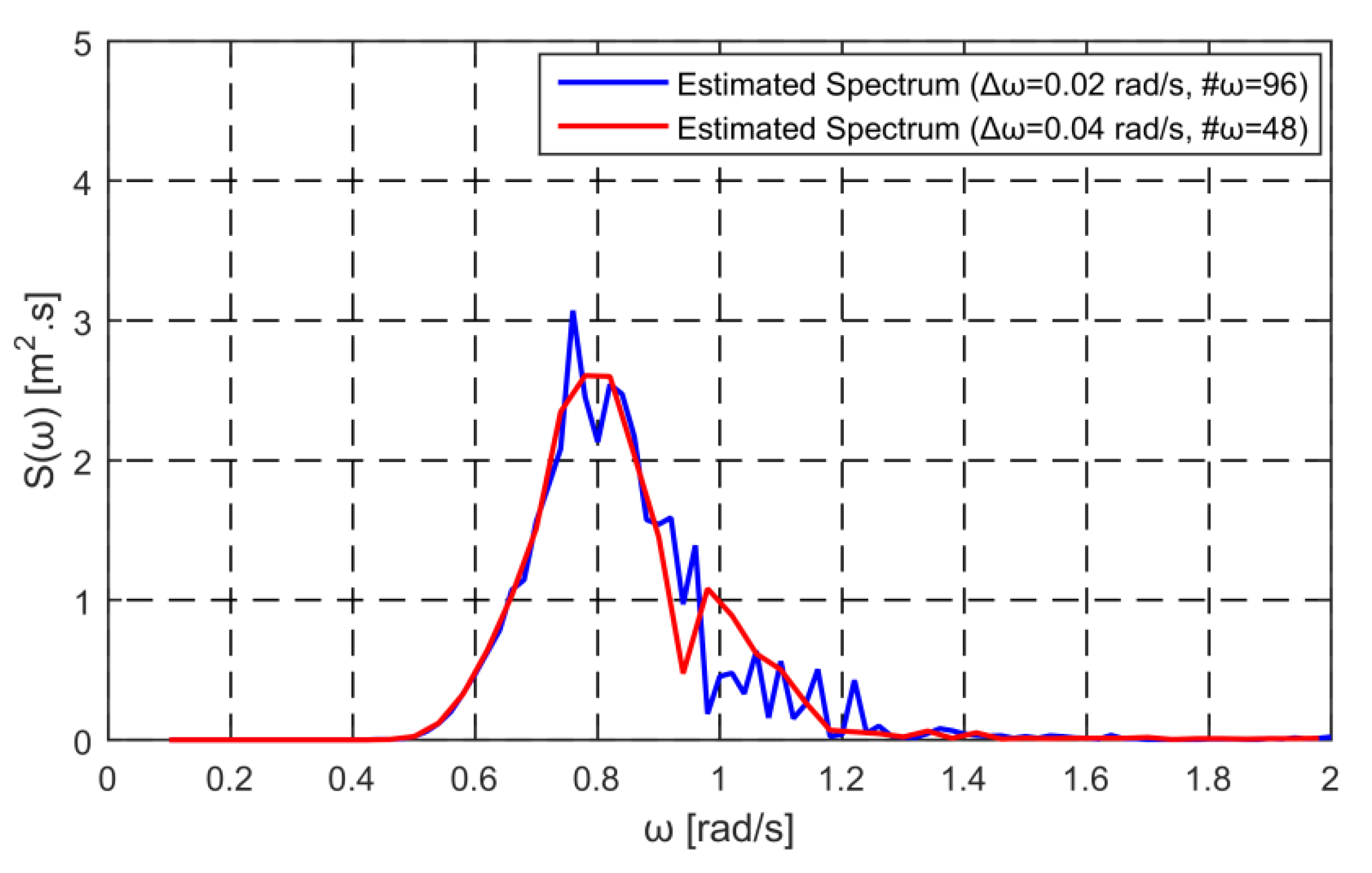
In this paper, the frequency range of 0.1~2.0 with 0.02 rad/s interval is used. Subsequently, the number of entry frequencies is 96 and the number of states to be obtained from the filter is 192. It was compared to the cases with different $\mathsf{\Delta }\omega$ to investigate the relationship between frequency intervals and estimation performance. Figure 21 shows that the real-time estimated wave spectra reasonably match, regardless of the two employed frequency intervals.

When superposing sinusoidal components, the randomly-perturbed frequency interval $\mathsf{\Delta }\omega$ was used by multiplying the random value $\alpha$, as shown below in order to prevent the signal repetition. The Kalman filter then ran for 1000 s.

$$\mathsf{\Delta }\omega =0.1\times \alpha [\mathrm{rad}/\mathrm{s}](-0.5\langle \alpha \langle 0.5)$$

(30)

Estimation tests were performed for various sea states to confirm whether the proposed modified TF can be applied to a wide range of applications. In the later part of this section, another vessel (OC4 semisubmersible e.g., [28,29]) with different RAO will be tested. The applied Kalman-filter technique equally worked well for the new vessel, which shows that the developed algorithm is not sensitive to vessel type either. To observe the sensitivity against various wave conditions, a series of sea states applied are shown in

Table 2. Simulated sea states and their parameters.

Sea State No.	Hs (m)	Tp (s)
1	1.5	6
2	5	9
3	9	11
4	13	13
5	17	15
6 (NP area in Figure 2)	1.5	18
7 (NA area in Figure 2)	13	11

, as below. In this table, No. 1 to 5 cases were selected as reasonable sea states [30]. On the other hand, No. 6 and 7 cases are particular sea states that correspnd to the two areas marked in Figure 2.

3.2. Results and Discussion

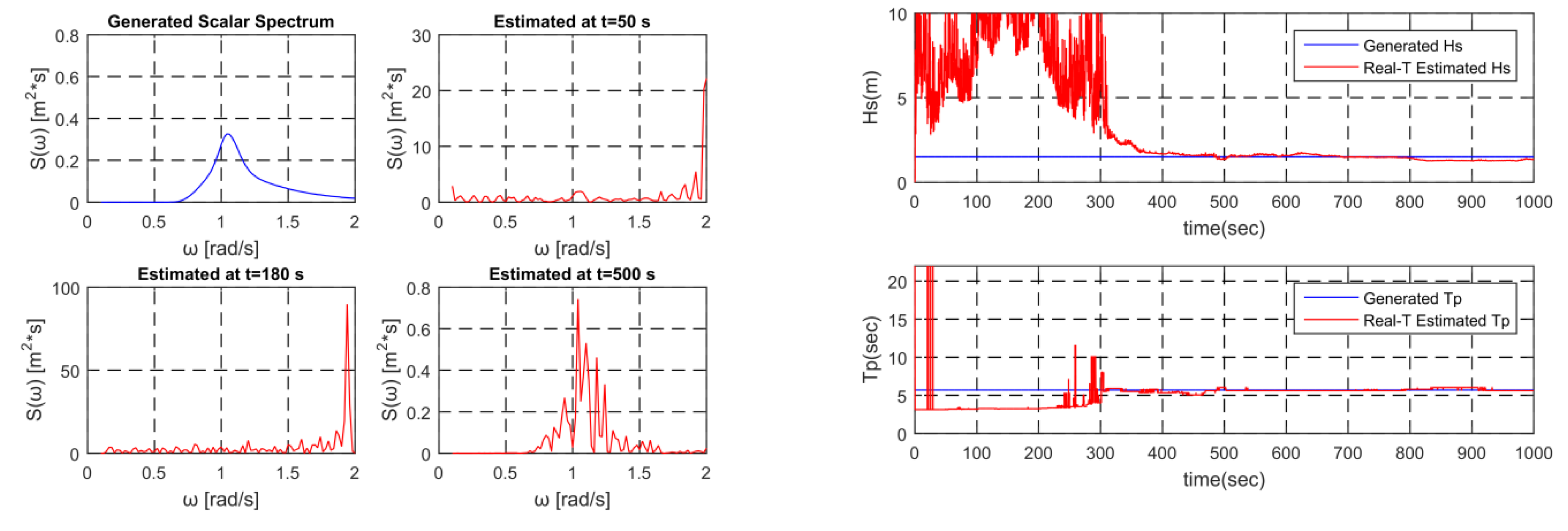
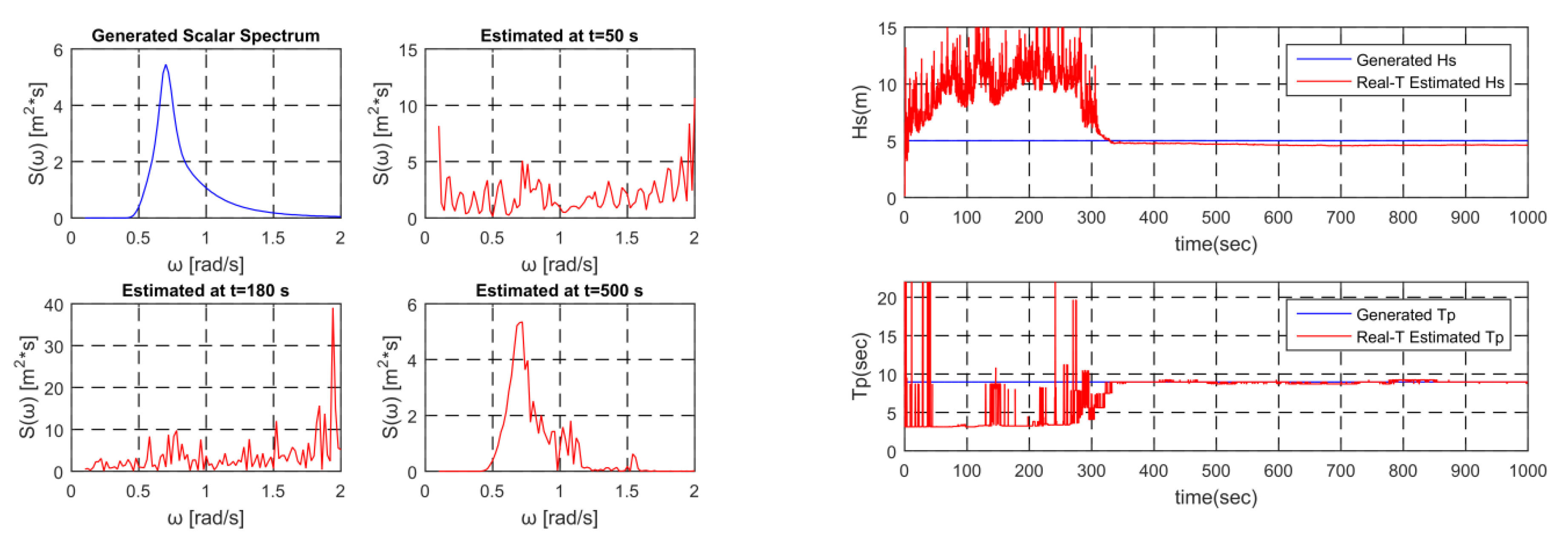
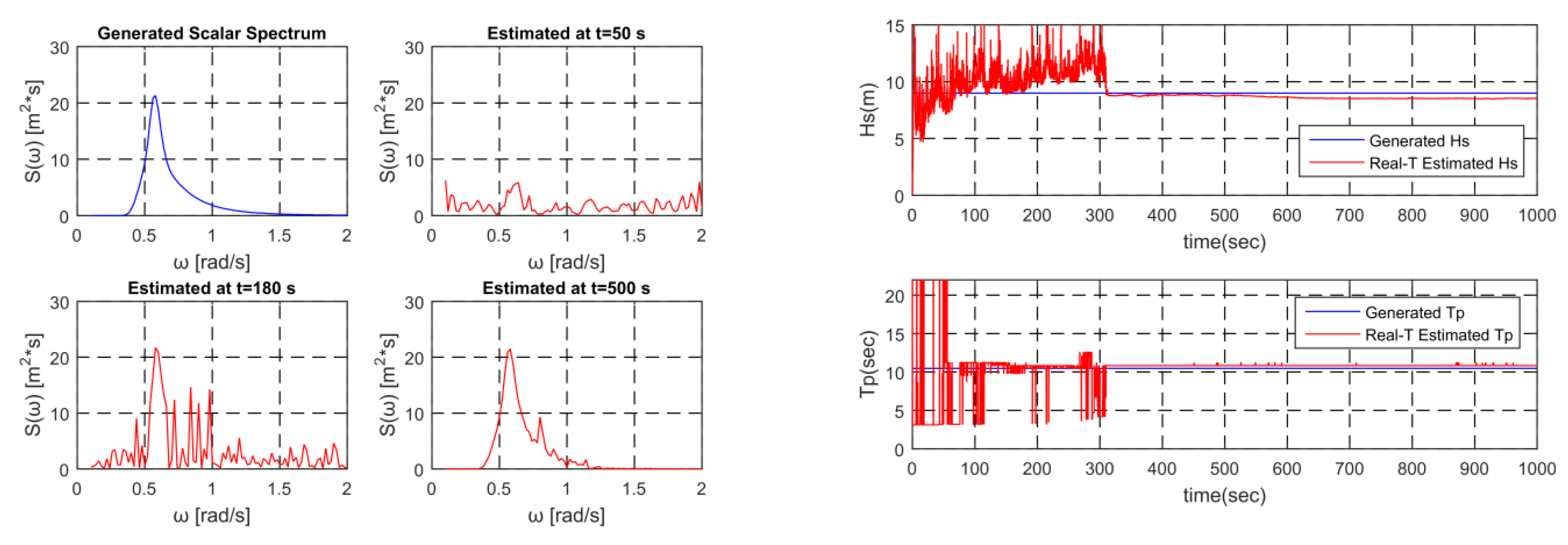
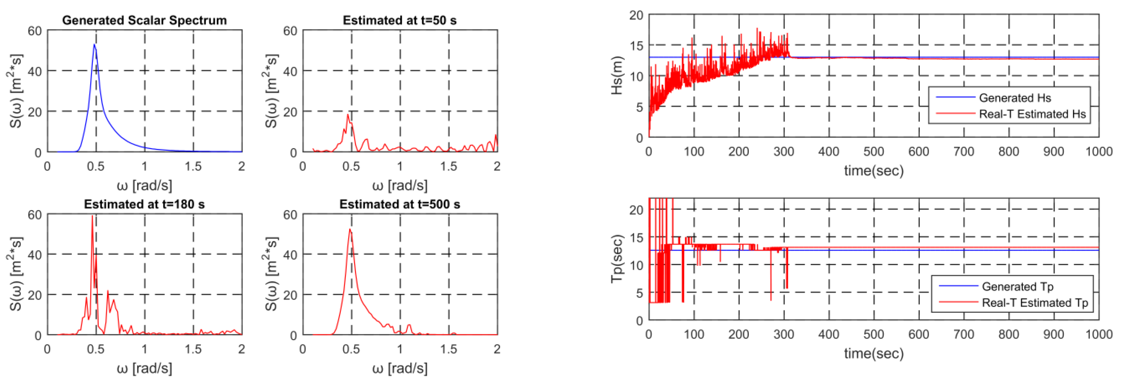
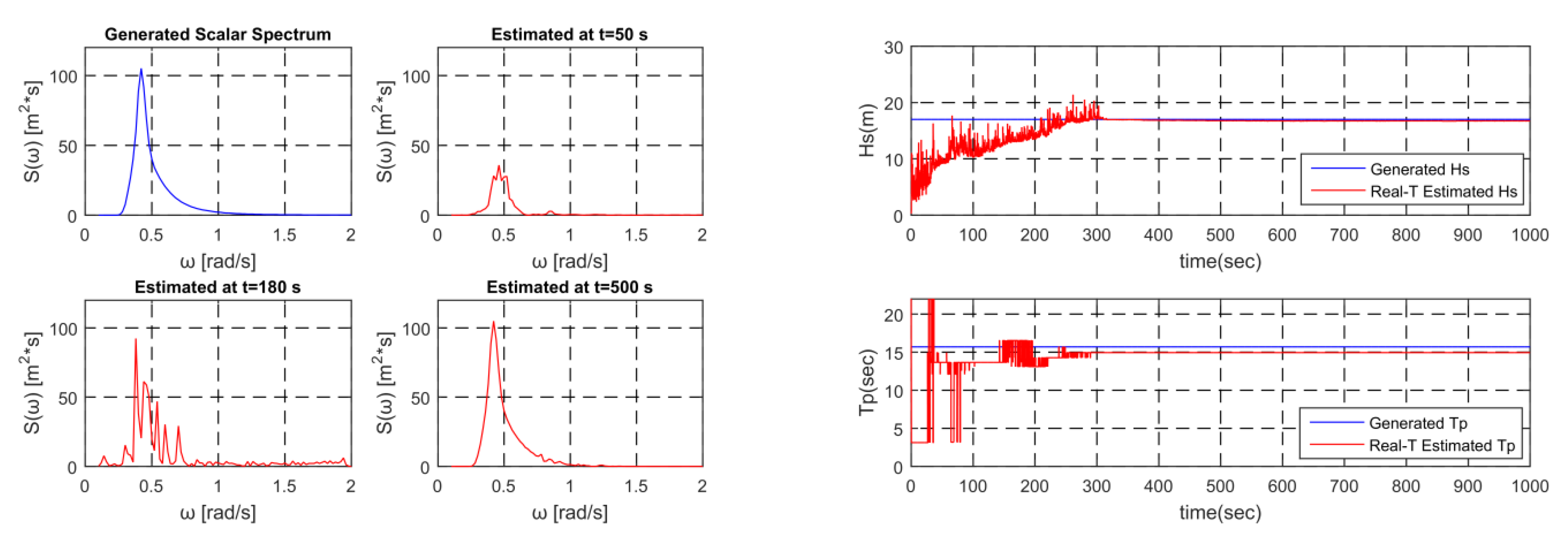
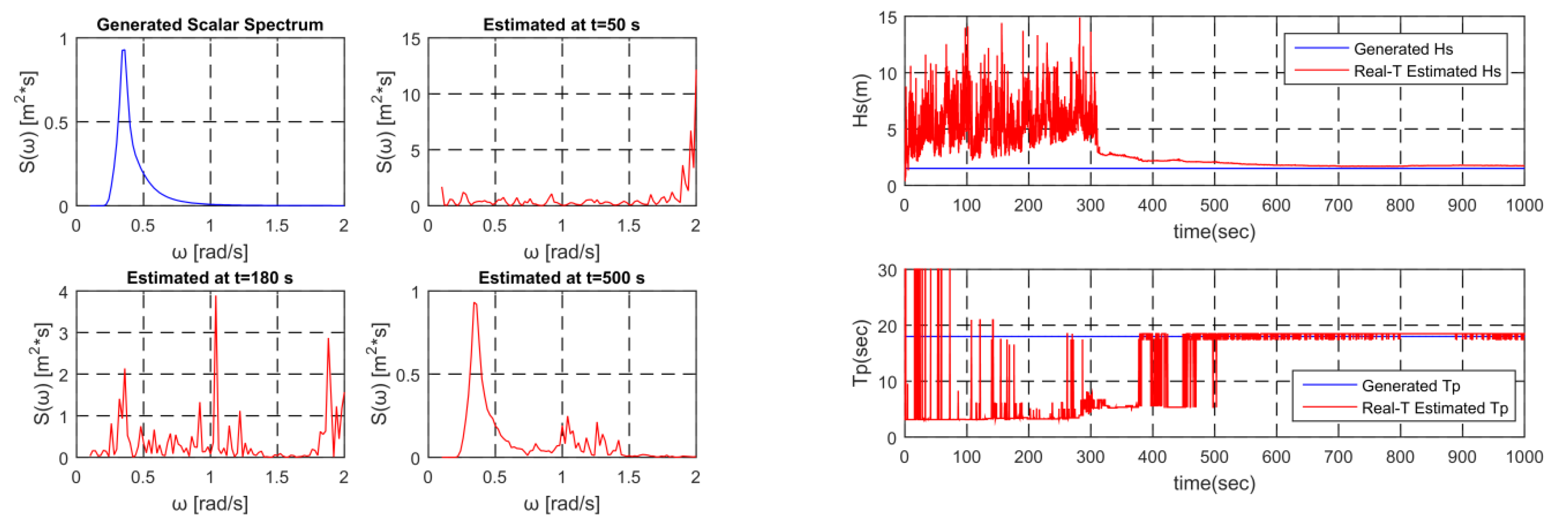
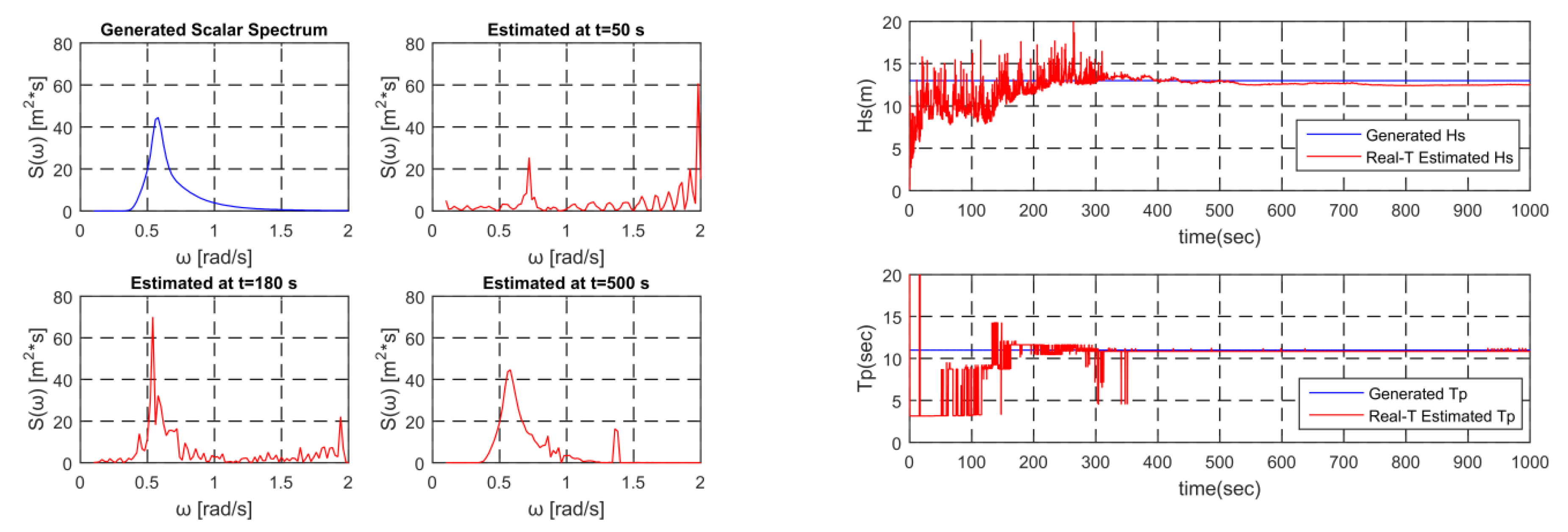
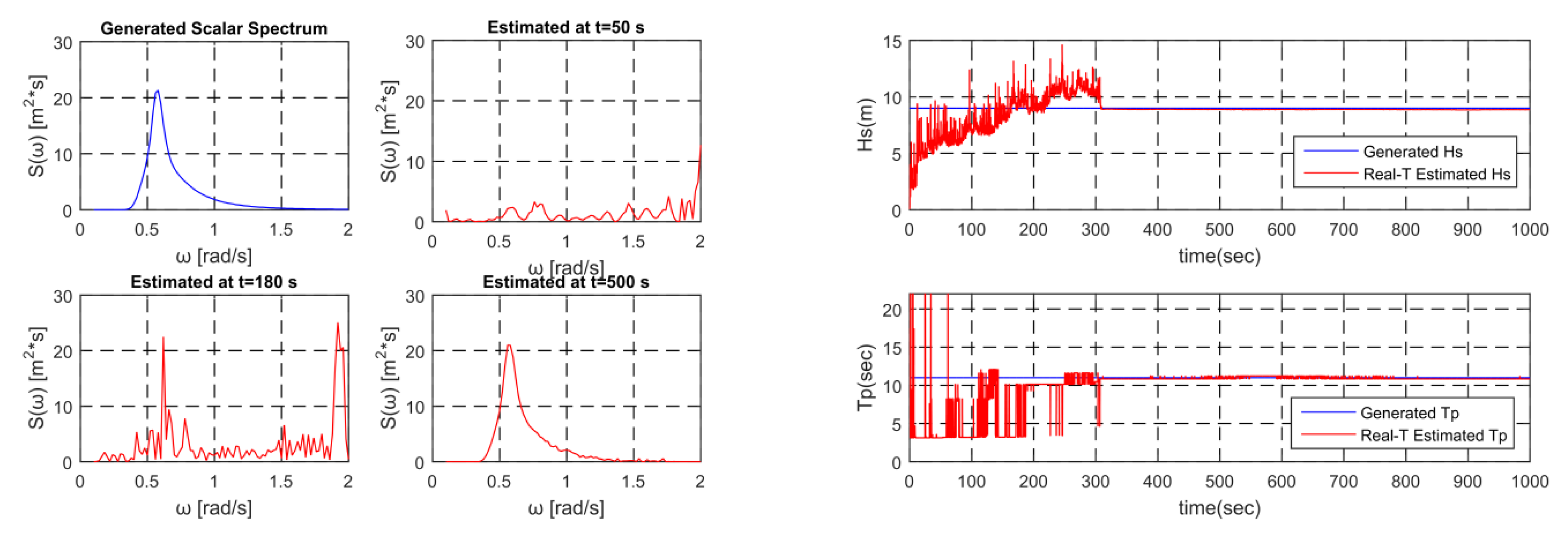
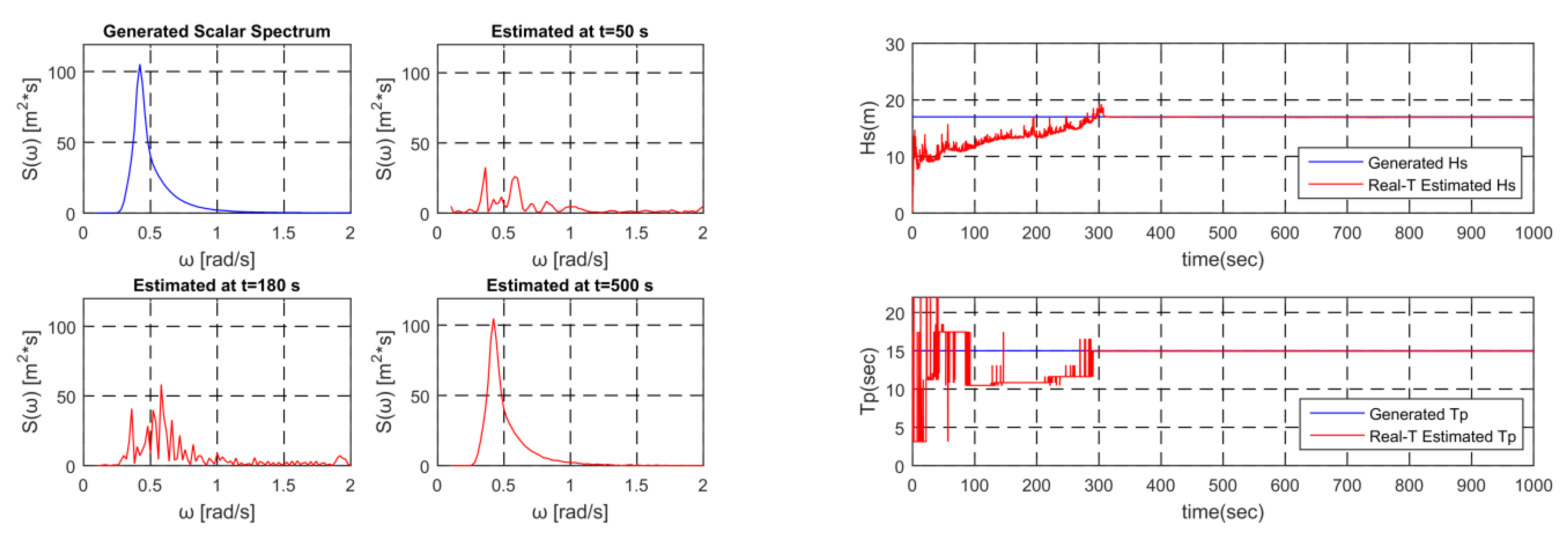
Figure 22, Figure 23, Figure 24, Figure 25, Figure 26, Figure 27 and Figure 28 present the results of the inversely estimated real-time spectra, Hs and Tp with time for the seven sea states when applying the proposed modified TF and adaptive R (Equation (14)) of [8]. It is seen that the developed Kalman filter technique works well for various sea states, which opens the door to a continuous inverse estimation of ocean waves from heave-motion sensor, regardless of sea states during service or voyage without adjusting the wave-frequency range and Kalman-filter parameters.

Next, we tested the developed modified Kalman-filter algorithm for another vessel (OC4 semisubmersible) to see whether the developed algorithms are sensitive to vessel types. In this regard, Figure 29 provide the motion TF of OC4 semisubmersible ([28,29]). Sea state No. 1, 3, and 5 were tested (Figure 30, Figure 31 and Figure 32) for the OC4. The estimation of real-time wave spectra, Hs, and Tp was good.

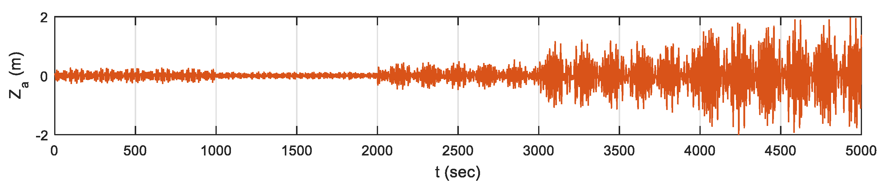
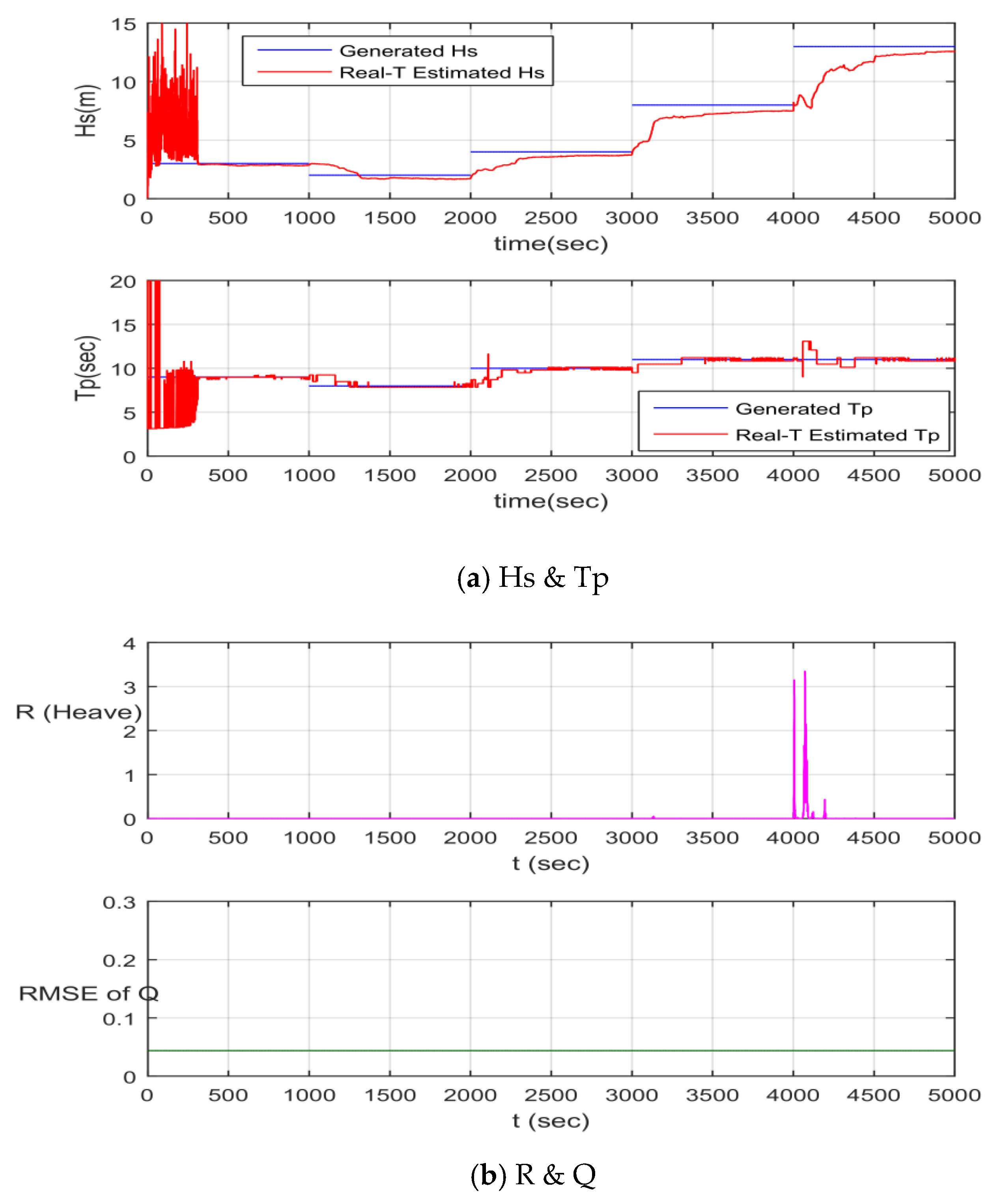
Up to this point, the developed Kalman-filter algorithm has been applied to the stationary sea state. However, sea states continue to change in actual sea, so, it is of interest to inversely estimate waves for non-stationary seas. The sea state sequence is set as shown in

Table 3. Simulated sea state sequence along the route.

Sequence	No. 1	No. 2	No. 3	No. 4	No. 5
Hs (m)	3	2	4	8	13
Tp (s)	9	8	10	11	11

, which is taken from a series of sea states along the dotted line from Jacksonville, Florida to the ‘NA’ point in Figure 2. It is assumed that the sea state is changing accordingly. The sensor error’s standard deviation was set as 2.3 cm and the modified TF was applied to the FPSO. Simulation was performed assuming that the vessel’s motion continuously varies due to the changes in sea state. The superposed motion time series for each sea state were then connected in order (Figure 33).

The algorithm was tested while using both modified TF and adaptive R. As a result (Figure 34), the real-time wave spectra are well estimated, even with drastic changes in sea states. Figure 34b shows the change in R and Q (fixed) during the estimation and Figure 35 is the RMSE of P, which is converging with more measurements.

4. Conclusions

Despite the inherent advantages of the Kalman filter, it has rarely been used for the inverse estimation of incident waves from motion sensors in the open literature. In the present paper, both real-time wave spectrum and elevation were obtained through the adaptive Kalman-filter algorithms.

A problem of amplified noise occurs in the zone associated with the Kalman filter when vessel’s motion RAO is small in the high frequency region and there is sensor error. A new solution to the problem is presented, so that the small gain in the RAO increases by a certain amount by using the Winer filter. If the proposed modified TF is applied, the overestimation of real-time wave spectra in the high-frequency region can be suppressed. The real-time incident wave profile can also be inversely estimated.

The vessel’s motion transfer functions and numerically generated motion-sensor signals were used to the present Kalman-filter processes. The Kalman filter has been tested for various sea states and different vessel types while using the modified TF through Wiener filter. The test results were promising.

In the forthcoming papers, the development is to be extended to multi-directional waves and the case with forward speed. The full-scale test with a real vessel in the real sea is also planned to further assess the developed Kalman-filter algorithms.

References

- Minter, A. Autonomous Ships Will Be Great. Available online: https://www.bloomberg.com/view/articles/2017-05-16/autonomous-ships-will-be-great (accessed on 12 July 2018).
- Jokioinen, E. Roadmap for Remote Controlled Ships. Available online: http://www.unmanned-ship.org/munin/wp-content/uploads/2015/06/MUNIN-Workshop-1-1-RR-Rolls-Royce%E2%80%99s-roadmap-for-autonomous-ships.pdf (accessed on 7 March 2019).
- International Maritime Organization. E-navigation. Available online: https://www.imo.org/en/ourwork/safety/navigation/pages/enavigation.aspx (accessed on 7 March 2019).
- Al-Habashneh, A.; Moloney, C.; Gill, E.W.; Huang, W.M. The Effect of Radar Ocean Surface Sampling on Wave Spectrum Estimation Using X-Band Marine Radar. IEEE Access 2018, 6, 17570–17585. [Google Scholar] [CrossRef]
- Jackson, F.C.; Walton, W.T.; Baker, P.L. Aircraft and satellite measurement of ocean wave directional spectra using scanning-beam microwave radars. J. Geophys. Res. Ocean. 1985, 90, 987–1004. [Google Scholar] [CrossRef]
- Gorman, R.M. Estimation of directional spectra from wave buoys for model validation. Procedia Iutam 2018, 26, 81–91. [Google Scholar] [CrossRef]
- Pascoal, R.; Perera, L.P.; Soares, C.G. Estimation of directional sea spectra from ship motions in sea trials. Ocean Eng. 2017, 132, 126–137. [Google Scholar] [CrossRef]
- Pascoal, R.; Soares, C.G. Kalman filtering of vessel motions for ocean wave directional spectrum estimation. Ocean Eng. 2009, 36, 477–488. [Google Scholar] [CrossRef]
- Nielsen, U.D.; Stredulinsky, D.C. Onboard sea state estimation based on measured ship motions. In Proceedings of the International Ship Stability Workshop, Washington, DC, USA, 1 January 2011; pp. 12–15. [Google Scholar]
- Svašek Hydraulics. NOAA Forecast Animations. Available online: http://www.worldwavedata.com/animations.html (accessed on 9 October 2018).
- Statista. Number of Ships in the World Merchant Fleet between January 1, 2008 and January 1, 2017, by Type. Available online: https://www.statista.com/statistics/264024/number-of-merchant-ships-worldwide-by-type/ (accessed on 12 July 2018).
- Brown, R.G.; Hwang, P.Y. Introduction to Random Signals and Applied Kalman Filtering; Wiley New York: Hoboken, NJ, USA, 1992; Volume 3. [Google Scholar]
- Simon, D. Using nonlinear Kalman filtering to estimate signals. Embed. Syst. Des. 2006, 19, 38. [Google Scholar]
- Ladetto, Q. On foot navigation: Continuous step calibration using both complementary recursive prediction and adaptive Kalman filtering. In Proceedings of the ION GPS, Salt Lake City, UT, USA, 19–22 September 2000; pp. 1735–1740. [Google Scholar]
- Bishop, G.; Welch, G. An introduction to the Kalman filter. In Proceedings of the Siggraph Course, Chapel Hill, NC, USA, 12 August 2001; Volume 8. [Google Scholar]
- Holzhuter, T. LQG approach for the high-precision track control of ships. IEEE Proc. Control Theory Appl. 1997, 144, 121–127. [Google Scholar] [CrossRef]
- SBG Systems. Ekinox Test Results. Available online: https://www.sbg-systems.com/wp-content/uploads/2018/07/Ekinox_Test_Marine.pdf (accessed on 7 March 2019).
- Kim, S.; Kim, M.-H. Dynamic behaviors of conventional SCR and lazy-wave SCR for FPSOs in deepwater. Ocean Eng. 2015, 106, 396–414. [Google Scholar] [CrossRef]
- Sundararajan, D. Digital Image Processing: A Signal Processing and Algorithmic Approach; Springer: Berlin/Heidelberg, Germany, 2017. [Google Scholar]
- Lagendijk, R.L.; Biemond, J. Basic methods for image restoration and identification. In The Essential Guide to Image Processing; Elsevier: Amsterdam, The Netherlands, 2009; pp. 323–348. [Google Scholar]
- Wikipedia. Wiener Filter. Available online: https://en.wikipedia.org/wiki/Wiener_filter (accessed on 4 June 2019).
- McAndrew, A. A Computational Introduction to Digital Image Processing; Chapman and Hall/CRC: Boca Raton, FL, USA, 2015. [Google Scholar]
- Pascoal, R.; Soares, C.G. Non-parametric wave spectral estimation using vessel motions. Appl. Ocean Res. 2008, 30, 46–53. [Google Scholar] [CrossRef]
- Pascoal, R.; Soares, C.G.; Sørensen, A. Ocean wave spectral estimation using vessel wave frequency motions. J. Offshore Mech. Arct. Eng. 2007, 129, 90–96. [Google Scholar] [CrossRef]
- Liu, S. An adaptive Kalman filter for dynamic estimation of harmonic signals. In Proceedings of the 8th International Conference on Harmonics and Quality of Power. Proceedings (Cat. No. 98EX227), Athens, Greece, 14–16 October 1998; pp. 636–640. [Google Scholar]
- Rhudy, M.B.; Salguero, R.A.; Holappa, K. A Kalman filtering tutorial for undergraduate students. Int. J. Comput. Sci. Eng. Surv. 2017, 8, 1–18. [Google Scholar] [CrossRef]
- Jin, C.; Kim, M.-H. Time-Domain Hydro-Elastic Analysis of a SFT (Submerged Floating Tunnel) with Mooring Lines under Extreme Wave and Seismic Excitations. Appl. Sci. 2018, 8, 2386. [Google Scholar] [CrossRef]
- Kim, H.; Kim, M. Comparison of simulated platform dynamics in steady/dynamic winds and irregular waves for OC4 semi-submersible 5MW wind-turbine against DeepCwind model-test results. Ocean Syst. Eng. 2016, 6, 1–21. [Google Scholar] [CrossRef]
- Kim, H.; Kim, M. Global Performances of a Semi-Submersible 5 MW Wind Turbine including Second-Order Wave-Diffraction Effects. Ocean Syst. Eng. 2015, 5, 139–160. [Google Scholar] [CrossRef]
- Veritas, N. Environmental Conditions and Environmental Loads; Det Norske Veritas: Oslo, Norway, 2000. [Google Scholar]
Figure 1.
Wave spectrum estimation process using Kalman filter.
Figure 2.
NOAA forecast snapshot for North West Atlantic [10].
Figure 3.
Kalman filter loop [12].
Figure 4.
Floating Production Storage and Offloading (FPSO) mesh (LPP (length between perpendiculars): 310 m, B: 47 m, Draft: 15 m).
Figure 5.
Heave transfer function of FPSO.
Figure 6.
Time series of heave motion with sensor noise.
Figure 7.
Generated and estimated spectrum/Evolution of parameters (Hs = 2 m, Tp = 7 s, Frequence: 0.1~1.15 rad/s).
Figure 8.
Generated and estimated spectrum/Evolution of parameters (Hs = 2 m, Tp = 7 s, Frequence: 0.1~2.0 rad/s).
Figure 9.
Comparison of error covariance and Kalman gain for frequency extension. (a) P (to 1.15 rad/s); (b) K (to 1.15 rad/s); (c) P (to 2.0 rad/s); (d) K (to 2.0 rad/s).
Figure 10.
Generated and estimated spectrum / Evolution of parameters using six motion (Hs = 2 m, Tp = 7 s, Frequence: 0.1~2.0 rad/s).
Figure 11.
Schematic diagram of noise amplification.
Figure 12.
Effect of Wiener filter.
Figure 13.
Effect of inverse of Wiener filter to compare to D(u,v).
Figure 14.
Comparison of Image Restoration and Wave Estimation.
Figure 15.
Modified Heave response amplitude operator (RAO) (red dotted line) of FPSO.
Figure 16.
Generated and estimated spectrum / Evolution of parameters using Modified TF (Hs = 2 m, Tp = 7 s, Frequence: 0.1~2.0 rad/s).
Figure 17.
Wave elevation estimation process using Kalman filter and Formula.
Figure 18.
(a) Input heave motion & (b) Estimated wave elevation using Modified TF (Hs = 2 m, Tp = 7 s, Frequence: 0.1~2.0 rad/s).
Figure 19.
Evolution of P.
Figure 20.
Error covariance and Kalman gain when using Modified TF, (a) P (to 2.0 rad/s); (b) K (to 2.0 rad/s).
Figure 21.
Comparison of estimated spectra averaged over 700~1000 s for the different number of frequency components.
Figure 22.
Generated and estimated spectrum/Evolution of parameters (Sea sate 1, Hs = 1.5 m, Tp = 6 s).
Figure 23.
Generated and estimated spectrum/Evolution of parameters (Sea sate 2, Hs = 5 m, Tp = 9 s).
Figure 24.
Generated and estimated spectrum/Evolution of parameters (Sea sate 3, Hs = 9 m, Tp = 11 s).
Figure 25.
Generated and estimated spectrum/Evolution of parameters (Sea sate 4, Hs = 13 m, Tp = 13 s).
Figure 26.
Generated and estimated spectrum/Evolution of parameters (Sea sate 5, Hs = 17 m, Tp = 15 s).
Figure 27.
Generated and estimated spectrum/Evolution of parameters (Sea sate 6, Hs = 1.5 m, Tp = 18 s).
Figure 28.
Generated and estimated spectrum/Evolution of parameters (Sea sate 7, Hs = 13 m, Tp = 11 s).
Figure 29.
Model and Modified Transfer Function of OC4.
Figure 30.
Figure 31.
Figure 32.
Figure 33.
Time series of heave motion during sea state change.
Figure 34.
(a) Evolution of parameters, (b) R (adaptive) and Q (fixed) during sea state change.
Figure 35.
Evolution of P during sea state change using Modified TF and Adaptive R.