Effectiveness of Automatic and Manual Calibration of an Office Building Energy Model

Featured Application

This work could contribute to evidence strengths and weaknesses of manual and automatic calibration of building dynamic simulation models leading at improving the quality of building retrofit solutions investigation.

Abstract

Energy reduction can benefit from the improvement of energy efficiency in buildings. For this purpose, simulation models can be used both as diagnostic and prognostic tools, reproducing the behaviour of the real building as accurately as possible. High modelling accuracy can be achieved only through calibration. Two approaches can be adopted—manual or automatic. Manual calibration consists of an iterative trial and error procedure that requires high skill and expertise of the modeler. Automatic calibration relies on mathematical and statistical methods that mostly use optimization algorithms to minimize the difference between measured and simulated data. This paper aims to compare a manual calibration procedure with an automatic calibration method developed by the authors, coupling dynamic simulation, sensitivity analysis and automatic optimization using IDA ICE, Matlab and GenOpt respectively. Differences, advantages and disadvantages are evidenced applying both methods to a dynamic simulation model of a real office building in Rome, Italy. Although both methods require high expertise from operators and showed good results in terms of accuracy, automatic calibration presents better performance and consistently helps with speeding up the procedure.

1. Introduction

The construction sector has a primary role in CO₂ reduction in Europe since buildings use around 40% of total energy consumption and generate almost 36% of greenhouse gases [1]. Recent data on world energy consumption in both residential and commercial buildings are presented by Allouhi et al., 2015 [2], together with an overview of measures and policies adopted by different countries for the reduction of energy consumption in buildings. They showed how in Asia, rapidly developing economies, essentially India and China, are looking to reduce the dramatic increase of energy consumption in buildings due to the fast urbanization rate [3].

Worldwide energy reduction will then benefit from the improvement of energy efficiency in buildings. This objective can be reached using two different and complementary approaches—measurements and simulations [4]. Simulation can be used to estimate the energy consumption of a building and consists of the construction of a virtual model of the building that has to reproduce the behaviour of the real building as accurately as possible. The reduction of the energy consumption can be pursued if the energy distribution throughout the building is known and understood. Building modelling can then be used both as a diagnostic tool, to better understand the physics laws of the building, and as a prognostic tool to predict the building’s behaviour once the laws are known. Building energy performance simulation (BEPS) can be achieved using data driven (black box) or law driven (white box) models. Considering the white box approach, many BEPS tools are available for example, TRNSYS, Energy Plus, DOE-2, ESPr, IDA ICE [5,6,7,8,9] and for the most popular, accurate capabilities evaluations and comparisons have been made [10]. Retrofit projects and operations management for buildings require accurate modelling that can be achieved through calibration. Calibration consists of an iterative process where model input is changed to reconcile the model output with the measured data. Although this process can be considered essential for having reliable results, still few practitioners are capable to perform it. Typical variables that are involved in the calibration process are mainly energy consumption [11,12,13,14] and indoor air temperature [11,15,16], for which simulated values are compared to measured ones on a specific time scale. Usually calibration at a small time scale (hourly of sub-hourly) results more difficult and time consuming than large scale such as annual and/or monthly rates. However, calibration with large time granularity (annual basis) can produce very good results while on a monthly basis can be affected by much larger errors. At present the most used statistical indices for the evaluation of the calibration accuracy are relative MBE (Mean Bias Error), RMSE (Root Mean Square Error), CVRMSE (Coefficient of Variation of RMSE) and NRMSE (Normalized RMSE), defined as follows [17,18,19]:

$$MBE=\frac{{{\displaystyle \sum }}_{i=1}^n{s}_i-m_i}{{{\displaystyle \sum }}_{i=1}^n{m}_i}\cdot 100\%$$

(1)

$$RMSE=\sqrt{\frac{{{\displaystyle \sum }}_{i=1}^n(s_i-m_i{)}^2}{n}}$$

(2)

$$CVRMSE=\frac{RMSE}{m_{mean}}\cdot 100\%$$

(3)

$$NRMSE=\frac{RMSE}{m_{max}-m_{min}}\cdot 100\%$$

(4)

where $s$ and $m$ refer to simulated and measured data respectively.

They are mostly evaluated for energy consumption, for which acceptance criteria have been introduced by various organizations as showed in

Table 1. Limits of MBE and CVRMSE for the calibration of building simulation models defined by different standard/guideline.

Standard/Guideline	Monthly Limit (%)		Hourly Limit (%)
	MBE	CVRMSE	MBE	CVRMSE
ASHRAE Guideline 14 [17]	±5	10	10	30
International Performance Measurement and Verification Protocol [18]	±20	-	10	20
Federal Energy Management Program [19]	±5	15	10	30

.

For what concerns the calibration performed with environmental variables, such as indoor air temperature, usually the model is considered calibrated when the RMSE is within the uncertainty of the measurements however no reference values of performance indexes are commonly provided. A wide piece of literature deals with BEPS calibration and this is confirmed also by reviews on this topic [20,21,22]. Substantially two approaches can be adopted for model calibration—manual approach and automatic approach.

Manual calibration consists of iterative and pragmatic process that involves the fine tuning of the input variables in a trial and error procedure. It uses building characteristics data from audit, energy use data and zone monitoring to get insight into the physical and operational characteristics of the building. The objective is to minimize the difference between measured and simulated output variables such as energy consumption, gathered from audit processes or inside temperature trends, obtained through environmental monitoring. Graphical techniques are widely used in manual calibration, as in the development of systematic and evidence based models [23]. Manual calibration requires high skill and expertise of the modeler that modifies the input basing principally on its experience. Apart from skill, the process usually requires a certain amount of time to be completed. Usually, to better understand the process, the input variables are changed one at a time then the simulation is run and for each simulation the output has to be compared with the original model. Many studies in the literature adopt manual calibration [23,24,25,26]. Manual calibration can also be used to gain detailed knowledge of the physical and operational characteristics of the buildings [27,28]. For example, Cornaro et al. 2016 [29] calibrated a model of a complex historical building and used manual calibration as a tool to identify various wall layers made by the superposition of unknown materials of different ages.

Automatic calibration relies on mathematical and statistical methods that mostly use optimization functions to minimize the difference between measured and simulated data. Many automatic procedures also include sensitivity analysis to reduce the number of input to the optimization tool and speed up the computing time [13,15,30,31,32]. Various algorithms have been used for the automatic calibration, among them the Bayesian approach [33], pattern-based approach [34], evolutionary algorithms [35,36] and particle swarm optimization [13,16,37]. In general, both automatic and manual calibration result either time consuming or costly methods. Manual calibration requires time of an experienced analyst while automatic calibration mainly requires computing power and time to complete the process. Therefore, it is difficult to determine whether one method could prevail over the other. Apart of a case in which the difference of the two approaches has been evidenced [38] the literature studies scarcely assess this issue. For this reason, it seems to the authors that the proposed evaluation, even if related to a specific case study, could be informative to the literature. This paper introduces an automatic calibration procedure developed by the authors that couples dynamic simulation and sensitivity analysis with automatic optimization using IDA ICE, Matlab and GenOpt respectively. This automatic calibration method has been compared to a manual procedure to evidence differences, advantages and disadvantages by applying both of them to a dynamic simulation model of a real office building in Rome, Italy. The comparison has been made in terms of accuracy of prediction of the real building consumption bills by the manual and automatic energy model calibrated using the temperature profile trends. Section 2 illustrates the methodology used to face the model calibration (both manual and automatic). Section 3 presents the case study, the monitoring campaigns and the model construction. Results regarding manual and automatic calibration are discussed in Section 4.

2. Materials and Methods

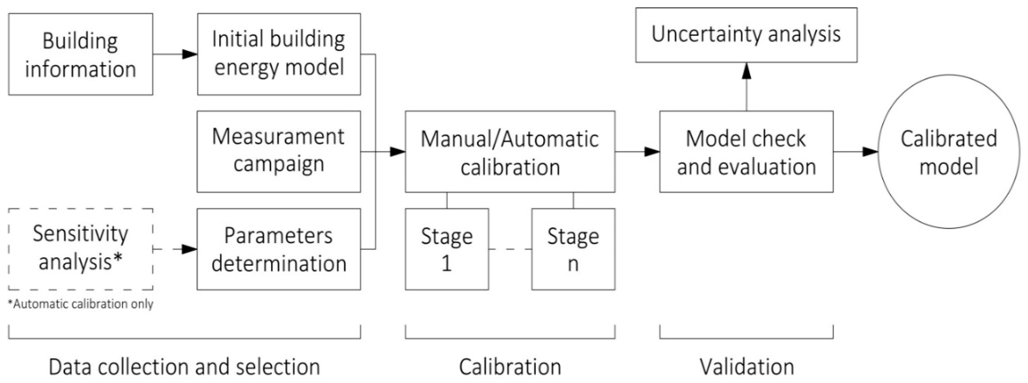
Both manual and automatic procedures consist of a first phase of data collection and selection, then a calibration phase and finally a check of the models through cross validation. The calibration phase was different according to the corresponding methodology. A multi-stage calibration process had been carried out for both approaches which involved firstly the envelope calibration and then the heating plant calibration using experimental data coming from short term monitoring campaigns carried out in different periods of the year [16,39]. The first step foresaw the use of the sensitivity analysis only for the automatic calibration. The whole process can be resumed as shown in Figure 1.

2.1. Data Collection and Selection

An initial dynamic building simulation model was developed and built with IDA-ICE 4.7.1 by EQUA Simulation [9], starting from the available information concerning the building. IDA ICE is a simulation application for the multi-zonal and dynamic study of indoor climate and energy use. IDA ICE can be used for complete energy and design studies, involving the envelope, systems, the plant and control strategies. The flexible architecture of the software allows to develop and to expand it with new capabilities. Additional features, like parametric simulation runs and visual scripting, support the user in a parametric design process. The coupling with optimization engines like GenOpt is available directly in the program.

From the original drawings, it had been possible to define the context, the geometry and the thermal zones of the building. According to the material properties, walls and roofs layers but also openings were specified.

Finally, plants, equipment and users-related data allowed the setting of the plant system (in terms of set points but also time schedules) and thermal gains.

Apart from the physical data related to the initial building model, other information were specifically required for the calibration procedure. To define the climate file involved in the simulation process for the calibration but also to obtain data to be compared with the simulation outputs, a measurement campaign had been settled. As multi-stage calibration was applied, a multi-phase campaign had been carried out.

Since the number of possible parameters influencing calibration was relatively high, a sensitive analysis using the Elementary Effect (EE) method, based on the Morris random sampling method [40], had been performed before the automatic calibration process identifying the most relevant ones.

Coupling MatLab with IDA-ICE, the EE method had been applied considering the hourly-simulated indoor temperature (T) for the period of each single stage of the whole calibration. According to the method, the number of EEs of each parameter (r), the number of parameters (k) and the number of levels (L) in which parameters range, were considered. A MatLab script was built that could open the IDA ICE environment iteratively, varying only one of the candidate inputs at each step while all the others were fixed to the previous value. N = r (k + 1) simulations had then been performed and the difference between simulated T and T from the initial guess model was expressed in terms of Mean Absolute Error (MAE). A single EE was defined as follows:

$$EE\left(x\right)=\frac{MAE\left(f\left(x_1,x_2,\dots ,x_i+\Delta x,\dots ,+x_k\right), f\left(x\right)\right)}{\Delta x}$$

(5)

where $f\left(x_1,x_2,\dots ,x_i+\Delta x,\dots ,+x_k\right)$ and $f\left(x\right)$ are T trends for current and first guess model respectively.

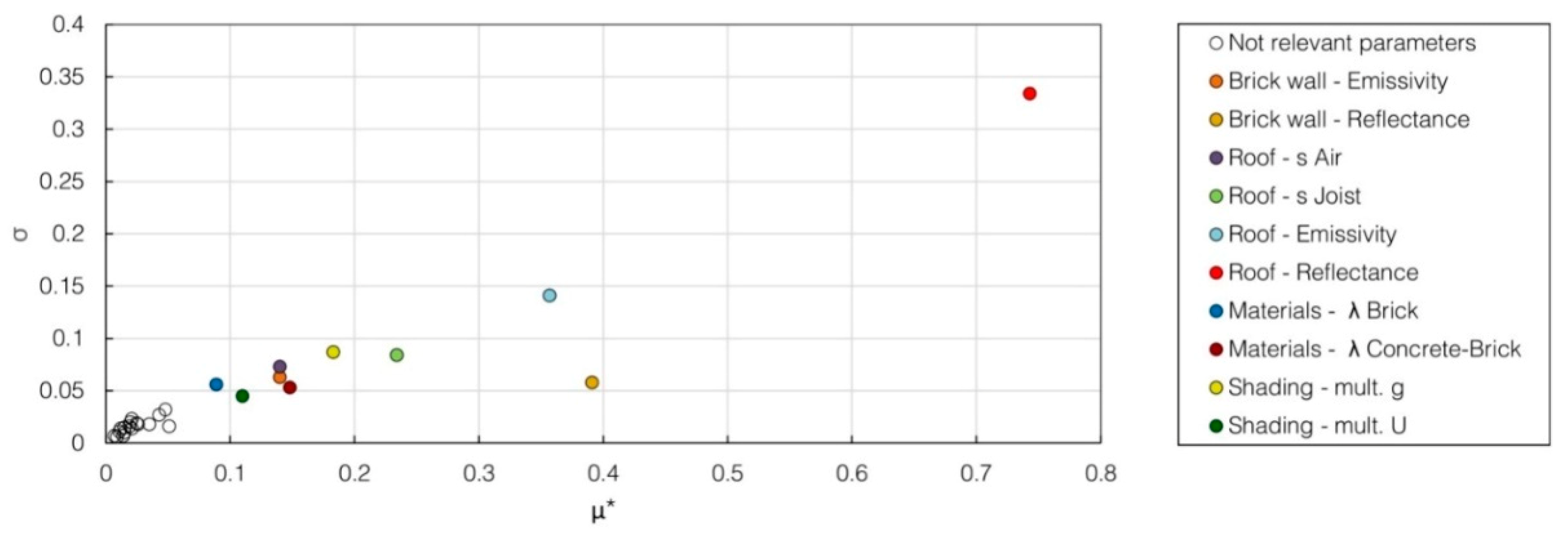
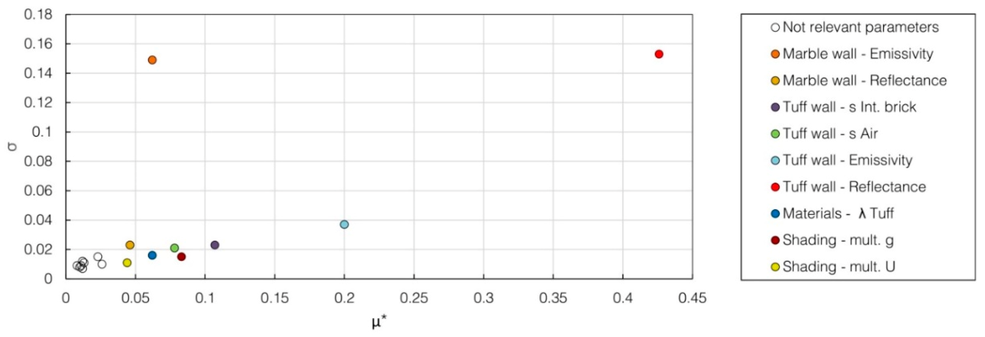
Absolute value of the mean (µ*), standard deviation (σ) of the distribution of the EEs and the ratio $\frac{\sigma }{\mu \ast }$ were finally evaluated. The relevance of the parameter was related to µ*, the larger µ* was, the more the corresponding input contributed to the dispersion of the output. σ was a measure of non-linear and/or interaction effects of the corresponding input. So, the ratio $\frac{\sigma }{\mu \ast }$ expressed the nature of the dependence of each parameter effect ($\frac{\sigma }{\mu \ast }$ < 0.1 linear, 0.1 ≤ $\frac{\sigma }{\mu \ast }$ < 0.5 monotonic, 0.5 ≤ $\frac{\sigma }{\mu \ast }$ < 1 almost monotonic, $\frac{\sigma }{\mu \ast }$ ≥ 1 not-linear and/or not-monotonic) [41].

2.2. Calibration

Although part of the logical procedure is similar, the calibration phase is treated separately according to the method involved.

The calibration was performed considering all the candidate parameters for minimizing the RMSE, CVRMSE and NRMSE between simulated and measured T. The manual and automatic procedures were carried out by two different master’s students with similar experience in building simulation modelling, supervised by a senior researcher.

2.2.1. Manual Calibration

In the manual procedure, the model was calibrated using the hourly indoor T measured in the different periods of the monitoring campaign.

The statistic parameters evaluated the goodness of the modification manually and iteratively applied to the model according to the experience of the operator and the observation of past steps.

In order to facilitate the assessment of the on-going calibration process, also other rating elements and strategies were involved. First, a graphic comparison of the plots for measured and simulated T was used to qualitatively estimate the direction of the iterative process. Analysis of heat balance and surface heat fluxes through walls, slabs and glazed surfaces helped to identify the most relevant construction elements in terms of heat transfer, determining the elements to be modified at each manual iterative step. Finally, Taylor’s diagram [42] was used to more completely evaluate the validity of the solutions found so far, using three statistical indexes—standard deviation (SD), correlation coefficient (R) and Centred RMSE (E’)—described by the following equations, respectively:

$$SD=\sqrt{\frac{{{\displaystyle \sum }}_{i=1}^n(x_i-x_{mean}{)}^2}{n}}$$

(6)

$$R=\sqrt{\frac{{{\displaystyle \sum }}_{i=1}^n\left(s_i-s_{mean}\right)\left(m_i-m_{mean}\right)}{S{D}_s\cdot S{D}_m}}$$

(7)

$$E^{\prime }=\sqrt{S{D}_s{}^2+S{D}_m{}^2-2\cos \left(S{D}_s{}^2\ast S{D}_m{}^2\ast R\right)}$$

(8)

where $x$ in $SD$ is a general parameter replaced by $s$ and $m$ in $S{D}_s$ and $S{D}_m$ respectively.

2.2.2. Automatic Calibration

In the automatic procedure, the model was again calibrated using the hourly indoor T measured in the different monitoring campaigns but involving simulation-based optimization method.

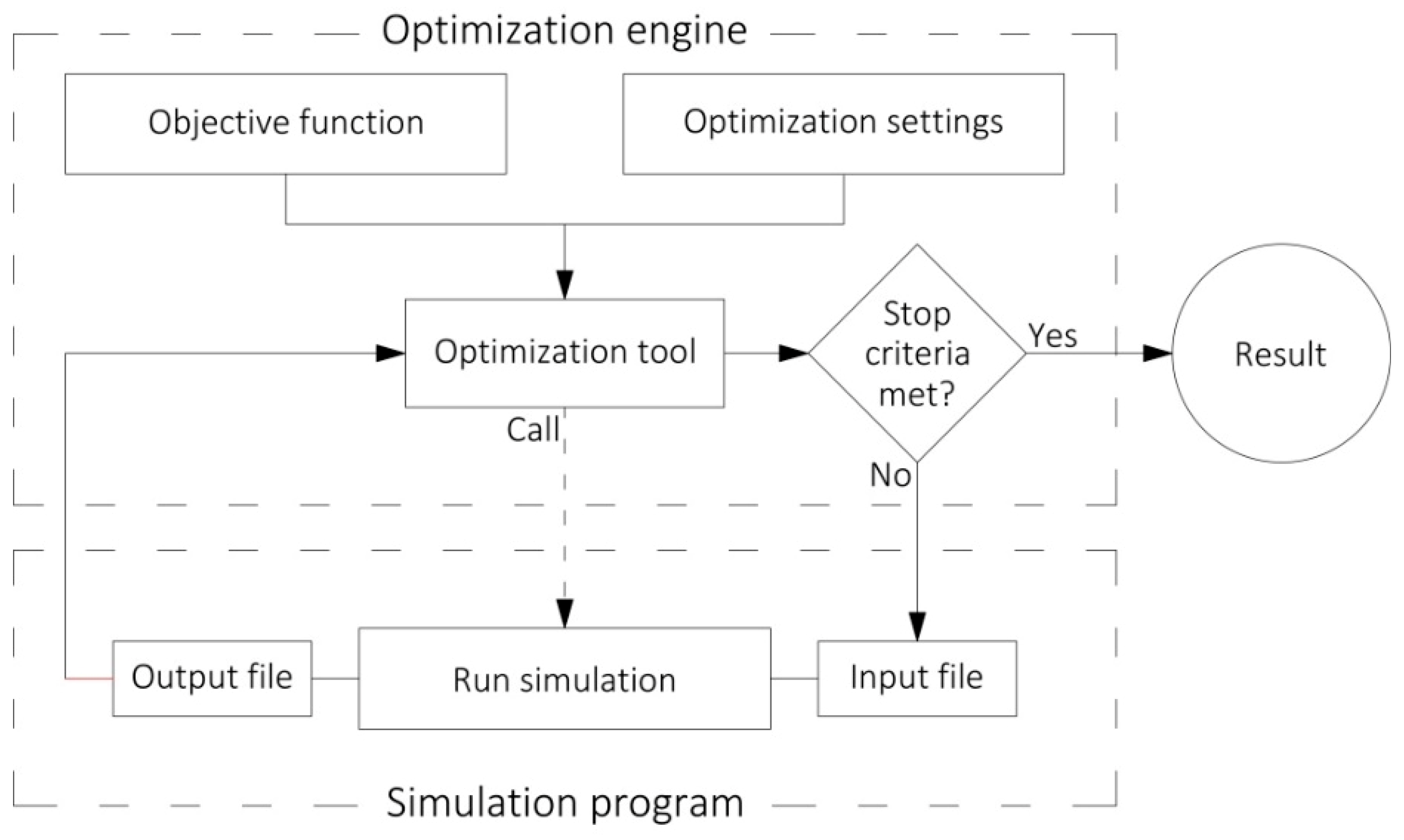
This automated method was based on the coupling of a simulation program and an optimization engine, which consists of several optimization algorithms. Optimization settings (variables, constraints, selected algorithm, etc.) and an objective function are needed for the optimization engine. Subsequently, the engine sends a call signal to the simulation program, to run a simulation and obtain a resulting scenario. If the output of the simulation satisfies the stop criteria for the algorithm, the optimal solution has been found and the process is concluded. Otherwise, the optimization engine elaborates and sends a new set of input data to the simulation program, calls for a new simulation run and repeats the process until at least a stop criterion is met (Figure 2).

In this calibration process, the objective function was the Cumulative Squared Error (CSE) of simulated (s) and measured (m) data:

$$CSE={\displaystyle \sum }_{i=1}^n{\left(s_i-m_i\right)}^2$$

(9)

The function was built in IDA-ICE including:

• Source-File, containing all the T data measured in a specific room for the monitoring campaign period;
• Zone-Sensor, referring to the thermal zone which the room corresponds, in order to extract the simulated T data to be compared with the measured ones;
• List of mathematical operators, to build the function.

Using GenOpt [43,44] via the parametric-runs macro embedded in the IDA ICE environment as the optimization engine, a hybrid algorithm—a combination of the Particle Swarm Optimization (PSO) algorithm for a first global search and the Hooke-Jeeves (HJ) algorithm for a second local search—minimized the objective function.

The PSO algorithm is a metaheuristic population-based algorithm that makes use of the group behaviour of an ensemble of particles, intended as a social organism. This “swarm” of particles searches in the solution space using simple rule-based decisions combined with randomized decisions, sharing information about the best solution found so far. The PSO algorithm does not require any previous knowledge of the objective function or its derivative, which allows it to deal with discontinuities. It can also search in very large search-spaces, does not “get stuck” in local optima and has the possibility to evaluate a large number of cost functions. However, although excellent solutions are always found by the algorithm, global optimum cannot be guaranteed [45,46].

The HJ algorithm is a direct search algorithm that, starting from a (user) selected base point, performs local search using a defined step in the variability range of the input parameters. If the process does not decrease the cost, the step is reduced and the search continues from the best solution found so far. If, conversely, the objective function decreases, a temporary best value is found and assumed as new base point for the following search. The process keeps on going until the cost function decreases. The HJ algorithm is not gradient-based—it can easily face discontinuities but may be attracted by local optima if the first base point has not been wisely selected [47].

The hybrid algorithm involved in the calibration process takes advantage of the positive face of both algorithms, reducing the disadvantages. Indeed, PSO rapidly converges to a set of very good solutions (potential optima), the best of which is taken as base point for HJ. Subsequently, the direct search algorithm more deeply investigates the neighbourhood of this base point, searching for the global optimum.

The calibration was performed as a single-objective optimization problem, considering only the candidate parameters derived from the sensitivity analysis. Once the process was over, the goodness of the result could be evaluated again in terms of RMSE, CVRMSE and NRMSE, also to facilitate the further comparison.

2.3. Building Description

The building selected for the case study is the administrative headquarter of the CIRM (acronym for International Radio Medical Centre), an organisation that deals with radio assistance and medical rescue services to international ships during navigation.

The structure, intended for office and outpatient use, was built in the early 1960s in Rome in the E.U.R district (latitude 41°49′48.3″ N, longitude 12°28′35.3″ E, altitude 30 m a.s.l.).

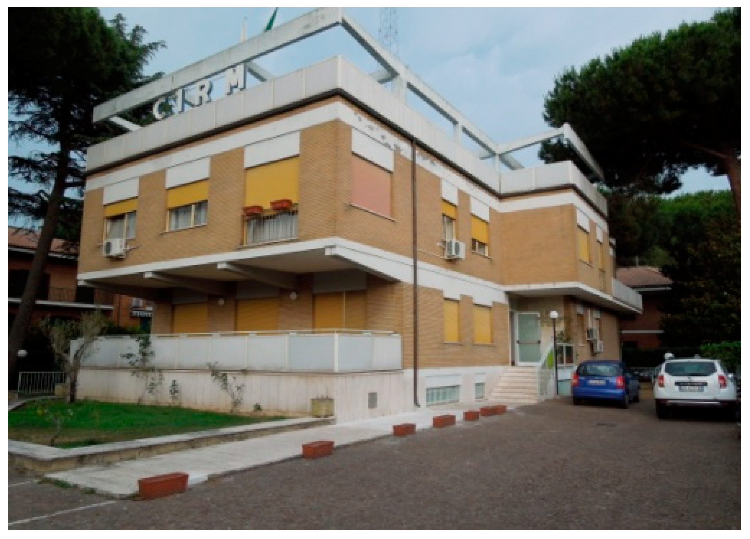
The building (Figure 3) consists of three floors—a basement (partially below the ground level on three sides), a ground floor and a first floor. The structure is a concrete frame, with bricks cladding and three different external finishes—exposed brick (ground and first floor), tuff blocks and white marble slabs in the southeast and north-west areas in the basement of the building, respectively. The total floor area is about 650 m² for a gross volume of approximately 2400 m³.

In winter, heating is provided by a centralised natural gas boiler with radiator, while for DHW (Domestic Hot Water) there are electric boilers. As regarding ground and first floor, independent air conditioners for cooling are available in a few rooms only.

The basement has been refurbished in the late 90 s, with new windows and radiators and the introduction of a HVAC centralized system for cooling. Ground and first floor are still in the original state. Since independent air conditioners for cooling are available in a few rooms only, and the centralized HVAC system was not active in the basement, the model was not calibrated for cooling, but the summer period was used to calibrate the building envelope.

2.4. Measurement Campaign

Modelling and calibration requested a monitoring campaign to measure both outdoor and indoor climate data. Outdoor measurements were carried out in order to use more representative climate data within the simulations. A portable measuring station was used.

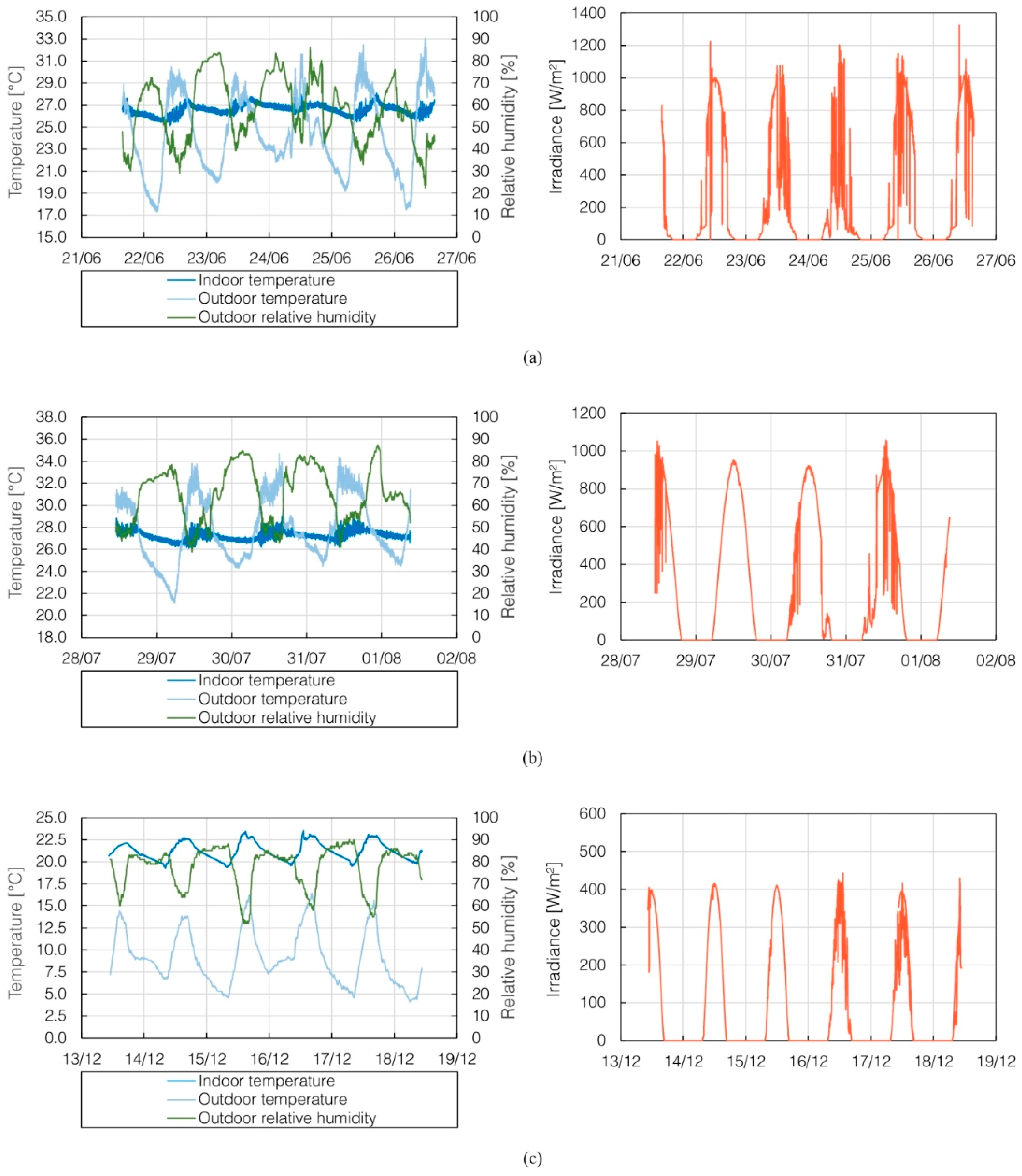
The station consisted of a copper anemometer (7911, Davis Instrument, Hayward, CA USA) with a wind speed range of 0.5–89 m/s and an accuracy of ±1 m/s for speed and ±7° for wind direction, a silicon solarimeter with a photodiode (SP Series Apogee Instruments) with a range of 0–350 mV and a sensitivity of 0.20 mV per W${\mathrm{m}}^{-2}$ and a thermo-hygrometer with an anti-radiation screen (Hygroclip2, Rotronic, Bassersdorf, Switzerland) with an accuracy of ±0.1 °C for temperature and ±0.8% for relative humidity. The same portable measuring system also provided an indoor station equipped with a thermo-hygrometer (Hygroclip2, Rotronic, Bassersdorf, Switzerland) with an accuracy of ±0.1 °C for temperature and ±0.8% for relative humidity, for indoor climate measurements. A control data logger (CR1000, Campbell Scientific, Logan, UT, USA), with 2 MB flash processor for the operating system, 4 MB SRAM, program memory and data memory, 16 analogic single-ended input, 100 Hz scan speed, ±0.06% of accuracy for analogic, was used to acquire both outdoor and indoor data at a one minute time rate. To obtain a larger spectrum of information about the building conditions, three measurement campaigns were carried out at different periods of the year and in different rooms. Outdoor air temperature, relative humidity, horizontal irradiance and indoor air temperature were collected in each survey (Figure 4). During the first period—Measurement Survey A (21–26 June 2015)—the outdoor station was on top of the building’s roof and the indoor station in a room of the first floor with northwest exposure. Figure 4 presents the environmental data recorded during the test period (Figure 4a).

In the second survey—Measurement Survey B (28 July–1 August 2015)—outdoor measurements were taken from a balcony on the first floor since it was not possible to reach the rooftop with the available cabling of the outdoor instruments connected with the indoor station that was located in a room in the basement with southeast exposure (Figure 4b).

For the third period—Measurement Survey C (13–18 December 2015)—again, due to logistic problems, only the indoor station was used. E.U.R district weather data, considered representative of the building’s surrounding environment were considered for outdoor data. The indoor measurement was taken in a room on the first floor with west exposure (Figure 4c).

During the three monitoring periods, the indoor measuring station was located in the centre of the reference room, far from walls, openings and direct heat sources (natural and artificial light, active equipment and plants), at a height of 1.5 m from the floor.

2.5. Energy Consumption

Bills of monthly natural gas consumption were available for calibration technique comparison. The consumption reported in the bills was estimated by the energy company using measured data from the past years and the outdoor ambient conditions of the referring period. Since delivered energy for fuel heating is expressed in IDA-ICE in kWh and the bills indicated the amount of monthly consumed gas in scm (standard cubic meters), to facilitate the comparison, a conversion of scm to kWh was carried out, considering (as reported in the bills) a GCV (Gross Calorific Value) of 39.64 MJ/m³ (

Table 2. Energy consumption data with conversion from scm to kWh.

Period	Measured Heating Fuel [scm]	Measured Heating Fuel [kWh]
1–27 November 2014	373	4107
28 November–23 December 2014	386	4250
24 December 2014–22 January 2015	441	4856
23 January–17 February 2015	394	4338
18 February–12 March 2015	332	3656
13 March–14 April 2015	365	4019
Total	2291	25,226

).

2.6. Model Construction

Starting from the drawing’s information and assuming part of the characteristic of the constructive elements from buildings of same typology and construction period (an inspection of wall layers was not allowed), a first guess of the model was built. The plant system was then modelled and added.

2.6.1. Envelope

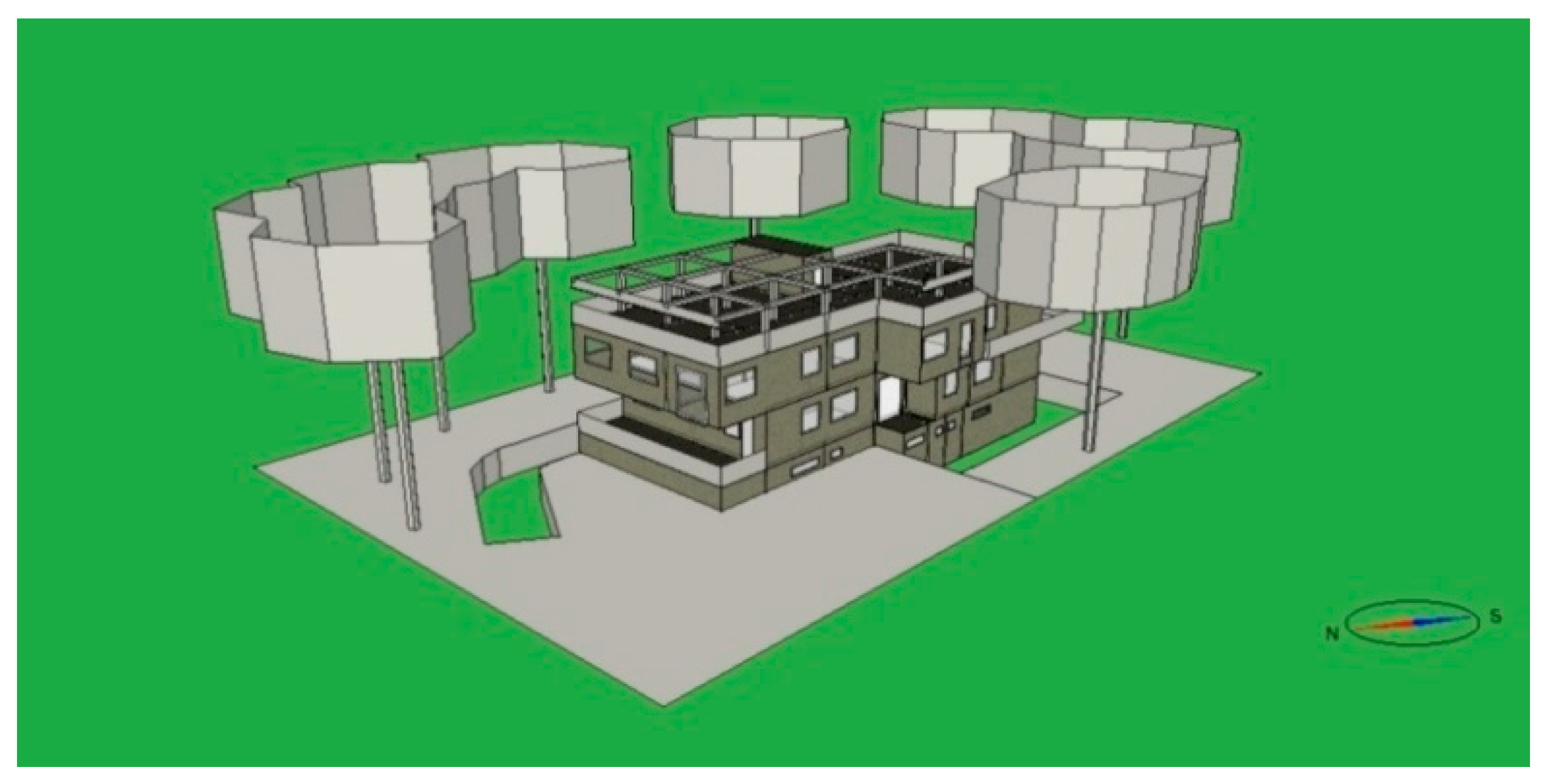
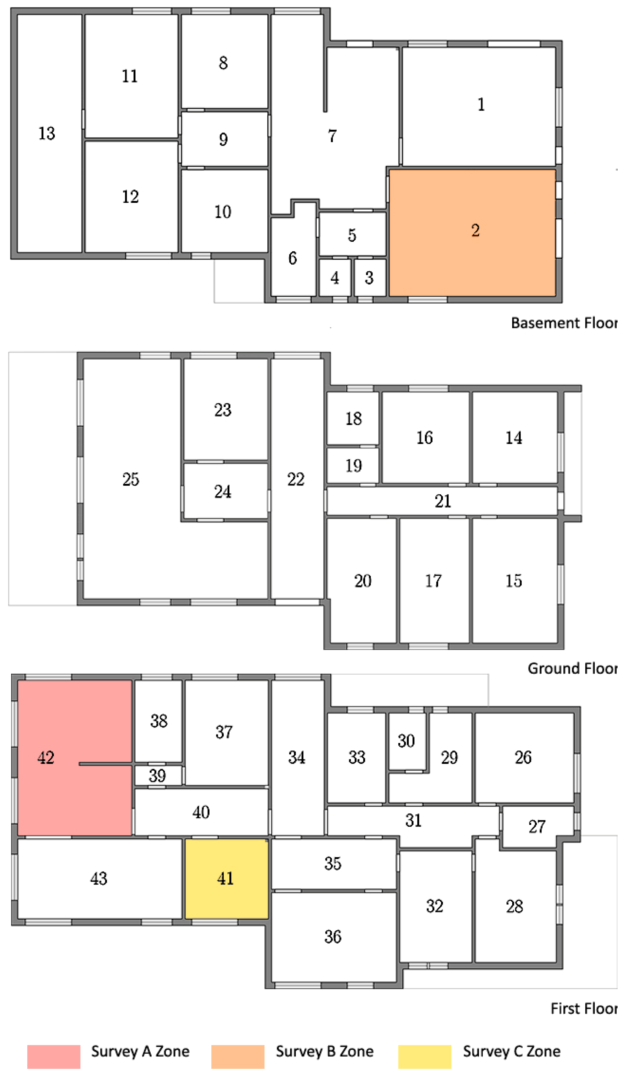
According to the original drawings, a geometrically representative and well oriented 3D model was built (Figure 5), including the high trees in the surroundings (for their shading effect), the excavated part of the garden and the division of each floor in several thermal zones, 43 in total (Figure 6) standing for the internal rooms. IDA-ICE’s database was uploaded with materials properties information to model the construction elements (

Table 3. Material properties for database upload in IDA-ICE for first guess model.

Material	Conductivity [W/mK]	Density [kg/m3]	Specific Heat [J/kgK]
Bituminous membrane	0.170	1200	1000
Cement mortar	1.400	2000	670
Concrete	1.060	1900	1000
Concrete-Brick	0.600	900	1000
Gravel	1.200	1700	1000
Gres	1.470	1700	710
Perforated Brick	0.387	690	840
Plaster	0.800	1800	790
Structural concrete	1.910	2400	1000
Tuff	0.550	1200	1000
White marble	3.000	2700	880
Wood	0.220	850	1660

).

Finally, concerning the construction elements, three different wall packages and three slab typologies were defined. Two windows and correspondent internal shading, one glazed internal door and two door types were specified (

Table 4. Construction elements for first guess model.

Doors
Element		s [cm]			Layer 1
Internal door		5			Wood
External door		7			Wood
Internal shading
Element		Multiplier ${\mathrm{U}}_{\mathrm{glass}}$ *	Multiplier ${\mathrm{g}}_{\mathrm{glass}}$ *		Multiplier T *	Diffusion factor
Refurbished roller blind		0.9	0.15		0.09	1
Original roller blind		0.9	0.15		0.09	1
Slabs
Element	s [cm]	Layer 1	Layer 2	Layer 3	Layer 4	Layer 5	Layer 6	U [W/m2K]
Basement floor	54.5	Gravel (40 cm)	Concrete (13 cm)	Gres (1.5 cm)	-	-	-	1.615
Internal floor	22.5	Plaster (1 cm)	Joist (12 cm)	Slab (4 cm)	Concrete (4 cm)	Gres (1.5 cm)	-	2.238
Roof	43	Plaster (1 cm)	Joist (16 cm)	Slab (4 cm)	Air (4 cm)	Concrete (7 cm)	Bituminous membrane (1 cm)	1.671
Surfaces
Element			Emissivity			Reflectance
External wall brick cladding			0.90			0.50
External wall marble cladding			0.90			0.50
External wall tuff cladding			0.90			0.50
Roof			0.90			0.50
Walls
Element		s [cm]	Layer 1	Layer 2	Layer 3	Layer 4	Layer 5	U [W/m2K]
External wall brick cladding		30	Plaster (2 cm)	Brick (12 cm)	Air (4 cm)	Brick (12 cm)		1.005
External wall marble cladding		34	Plaster (2 cm)	Brick (12 cm)	Air (4 cm)	Brick (8 cm)	Marble (4 cm)	1.041
External wall tuff cladding		30	Plaster (2 cm)	Brick (12 cm)	Air (4 cm)	Tuff (12 cm)		1.043
Windows
Element		${\mathrm{U}}_{\mathrm{glass}}$ [W/m2K]	${\mathrm{U}}_{\mathrm{frame}}$ [W/m2K]		${\mathrm{g}}_{\mathrm{glass}}$	T	Internal shading
Refurbished Window		2.6	2		0.39	0.31	Refurbished roller blind
Original Window		5.8	3		0.59	0.48	Original roller blind
Glazed doors		5.8	5.2		0.59	0.48	-

* IDA ICE considers the effect of internal shading modifying (through a multiplier) the main window properties: glass thermal transmittance (${\mathrm{U}}_{\mathrm{glass}}$), glass solar gain (${\mathrm{g}}_{\mathrm{glass}}$) and solar transmittance (T).

). Thermal bridges and infiltrations settled on typical values as shown in

Table 5. Infiltration and thermal bridges.

Infiltrations
Element	Air tightness [ACH *]
Wind driven flow	0.5
Thermal Bridges
Element 1	Element 2	Linear transmittance of thermal bridge [W/mK]
External wall	Internal wall	0.03
External wall	External wall	0.08
External windows perimeter	-	0.03
External doors perimeter	-	0.03
Roof	External wall	0.09
Roof	Internal wall	0.03

* Air Change per Hour.

.

The first guess model was adopted as starting point for both calibration processes.

2.6.2. Plant

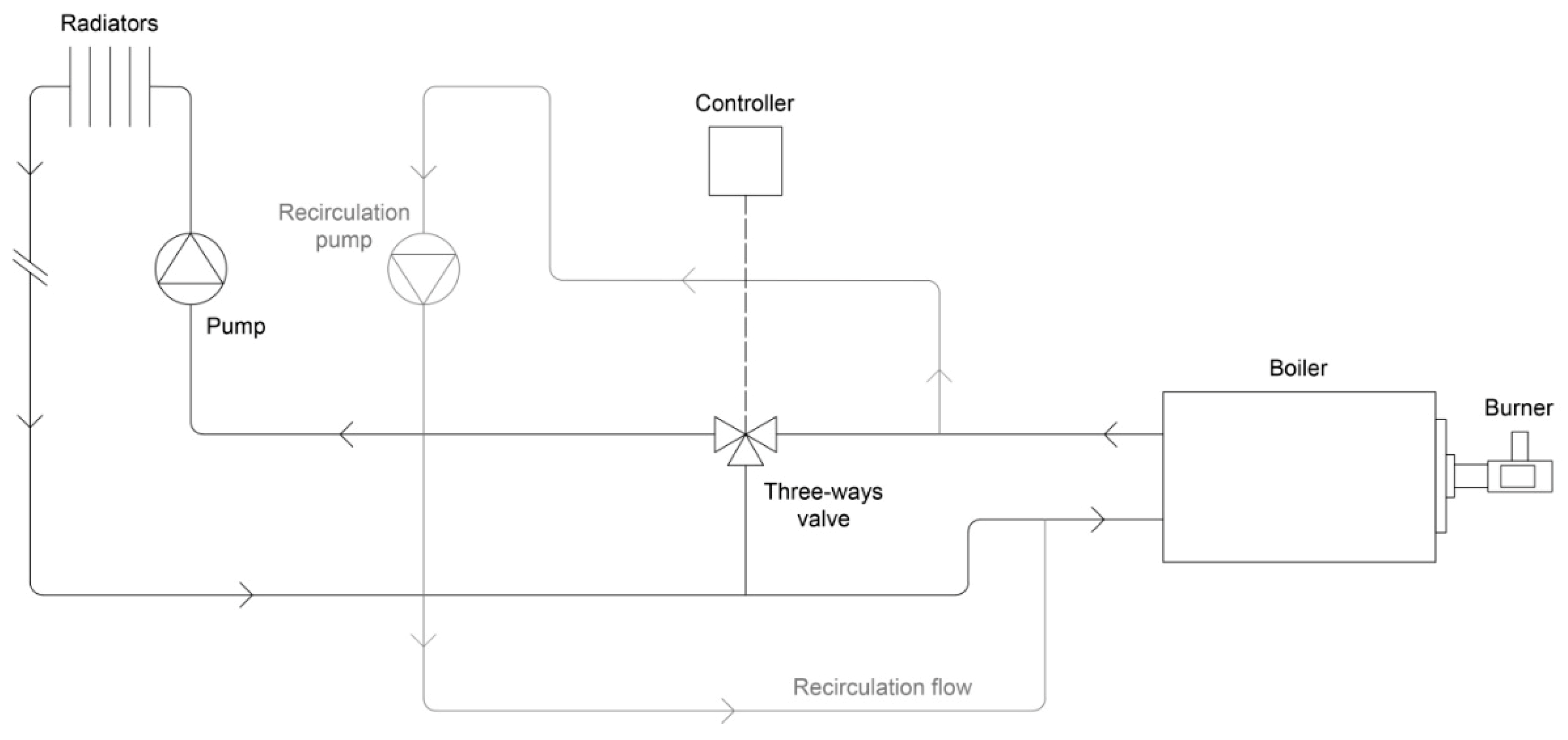
The plant model referred to the heating system only, which consists of a boiler, several water radiators (almost one in each room/thermal zone) and a controller for the three-ways valve. (Figure 7).

According to the operating manual, the burner-boiler system was given a 200 kW maximum heating capacity and an efficiency of 0.93.

Concerning the water radiators, emitted power is dynamically calculated by IDA-ICE as follows:

$$P=K\cdot l\cdot d{T}^N$$

(11)

where $l$ is the length of the radiator, $dT$ is the instantaneous temperature difference between the water and the zone air, $K$ is the emitted power per unit of equipment length, $N$ is an exponent that, as $K$, depends on the material and the structure of the radiator.

For the radiators at the basement level, according to the manual, it had been possible to determine all the technical specifications. A single element of 0.08$·$0.08$·$0.77 m³, at $\Delta \mathrm{T}$ = 50 °C, was given an exponent coefficient of $N=1.339$ and a maximum power at capacity of 147.4 W (total value depends only on the radiator length).

For radiators at ground and first floor level, since technical data were not available, a first guess of $N=1.28$ (typical for ordinary radiators) was given and maximum power at capacity was calculated as suggested in UNI 10200 [48]:

$$P=314\cdot S+C\cdot V$$

(12)

where $S$ is the external convection surface, $V$ is the volume of the radiator and $C$ is an experimental parameter related to the material and typology of the equipment (for finned steel radiators the given value is $C=22500$ at $\Delta \mathrm{T}$ = 60 °C).

At the three-ways valve, supplied water can be mixed with return water in order to adjust water temperature to reach desired ambient conditions. The controller is supposed to manage the valve according to a preselected heating curve (coupled values of outdoor T and supplied water T), attempting to reach a desired indoor ambient temperature set point (25 °C). It has to be noted that, since the two calibrations have been carried out by different operators, in the manual calibration a standard heating curve provided by IDA ICE has been considered while for the automatic calibration the real heating curve from the controller specifications has been used (water T = 90 °C for outdoor T = −2.5 °C and water T = 35 °C for outdoor T = 20 °C).

During the winter, heating system is on all days according to working hours schedule (8:00–17:00).

2.6.3. Occupancy, Equipment and Lights

Occupancy, equipment and lights were generally scheduled as present/on according to working hours (all days 8:00–17:00). Occupants were considered to have a metabolic rate of 1.2 MET; nevertheless, only 11 over 44 rooms (office rooms) were constantly occupied during working hours. Other rooms’ occupancy (meeting rooms, ambulatory, archive, etc.) was considered as not influential. Equipment basically consists of working station (computer, monitor, printer, etc.) which power (related to its thermal gain) was estimated to be 100 to 200 W and has been object of further calibration. Each lighting element was given a power of 100 W.

3. Results

Both manual and automatic calibration were performed for the correct modelling of the CIRM administrative headquarters building. Both calibration methods included multi-stage process. Three tuning phases, according to the three monitoring period, were in fact involved in the processes:

• Calibration A (first floor): using five days of summer data (22–26 June), a first tuning was given to the building envelope. Calibration was performed referring to an office room situated in the north part of the first floor of the building. No occupants were included, and lights, equipment and plants were turned off.
• Calibration B (basement): using a further five days of summer data (28 July–1 August), a second building envelope tuning was performed. Calibration referred to a conference room situated in the south part of the basement. Again, no occupants, lights, equipment and plants were considered.
• Calibration C (heating system): using five days of winter data (14–18 December), the heating system was tuned. Calibration was related to a north-west office room situated in the first floor. Internal gains due to occupants, equipment and lights were scheduled according to working time during the day.

Calibration A and C, due to adjustments of monitoring instruments and room conditions during initial phases of the campaigns, started from the second monitored day. Since different operators carried out the two calibration processes in parallel, apart from the results of each step, the strategies adopted were sometimes different. Regarding the computational time both procedures were executed with a PC equipped with a quad core i7-2600 (3.4 GHz) processor and 8 GB RAM.

3.1. Manual Calibration

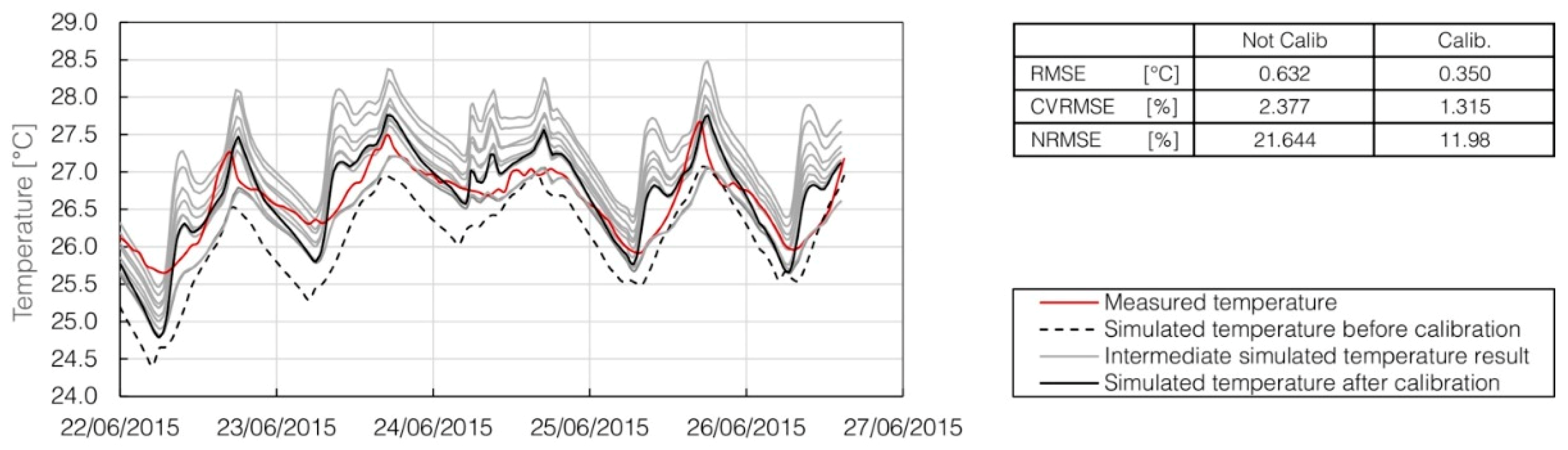
3.1.1. Calibration A (First Floor)

Calibration A aimed to provide a first tuning to the building envelope, focusing on the ground and first floors. The process involved parameters related to external wall with brick cladding (layers and bricks conductivity), covering roof (layers), integrated windows shading for original windows (multiplier for glass conductivity and solar gain), thermal bridges and infiltrations (

Table 6. Parameters collection for Calibration A *.

Reference	Element	First Guess	Lower Bound	Upper Bound
Linear Transmittance of Thermal Bridges	Ext. Wall-Int. Wall [W/(K⋅m)]	0.03	0.025	0.035
	Ext. Wall-Ext. Wall [W/(K⋅m)]	0.08	0.06	0.09
	Window Perimeter [W/(K⋅m)]	0.03	0.025	0.035
	Door Perimeter [W/(K⋅m)]	0.03	0.025	0.035
	Ext. Wall-Roof [W/(K⋅m)]	0.09	0.07	0.10
	Int.Wall-Roof [W/(K⋅m)]	0.03	0.025	0.035
Infiltration	ACH	0.5	0.5	1.0
Ext. Wall-Brick	s Int. Brick [m]	0.12	0.08	0.12
	s Air [m]	0.04	0.03	0.05
	s Ext. Brick [m]	0.12	0.08	0.12
Roof	s Screed [m]	0.07	0.07	0.09
	s Air [m]	0.04	0.04	0.08
	s Joist [m]	0.16	0.16	0.24
Material Properties	λ Brick [W/(m⋅K)]	0.387	0.387	0.472
Shading (original windows)	mult. g	0.15	0.15	0.4
	mult. U	0.9	0.8	1
	D	1	0.5	1

* s = thickness, λ = thermal conductivity, mult. g = multiplier for glass solar gain, mult. U = multiplier for glass thermal transmittance, D = diffusion factor.

).

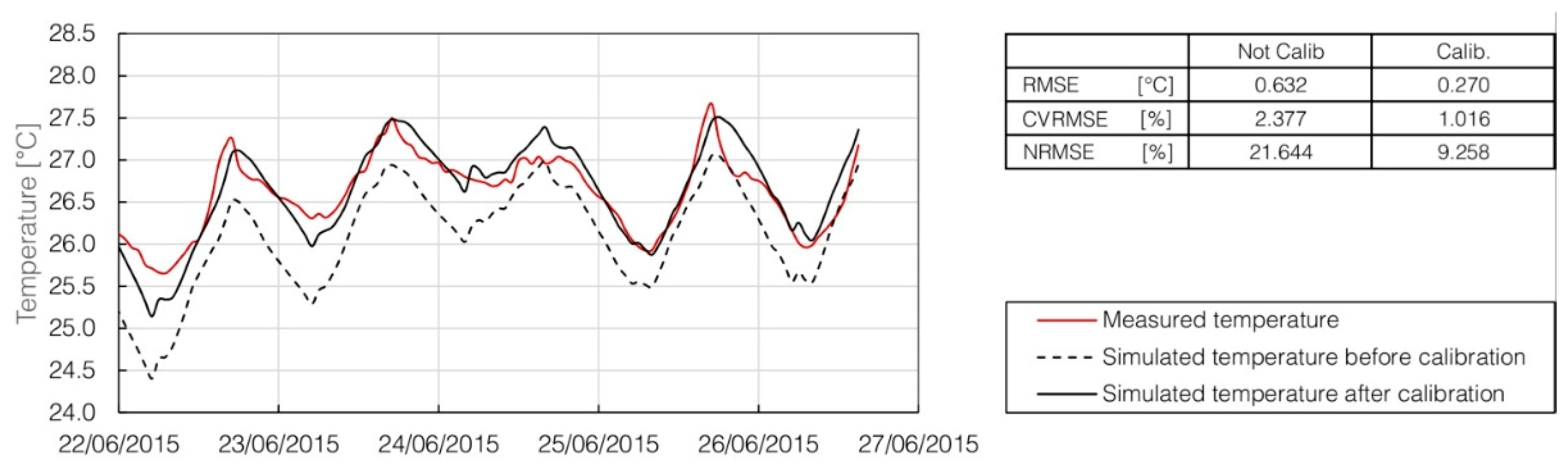
The calibration required over 1 month of work and attempts to achieve the final solution. Figure 8 shows the output of the most representative simulations (51), where the sole run time of each simulation took 5–7 min to be completed.

3.1.2. Calibration B (Basement)

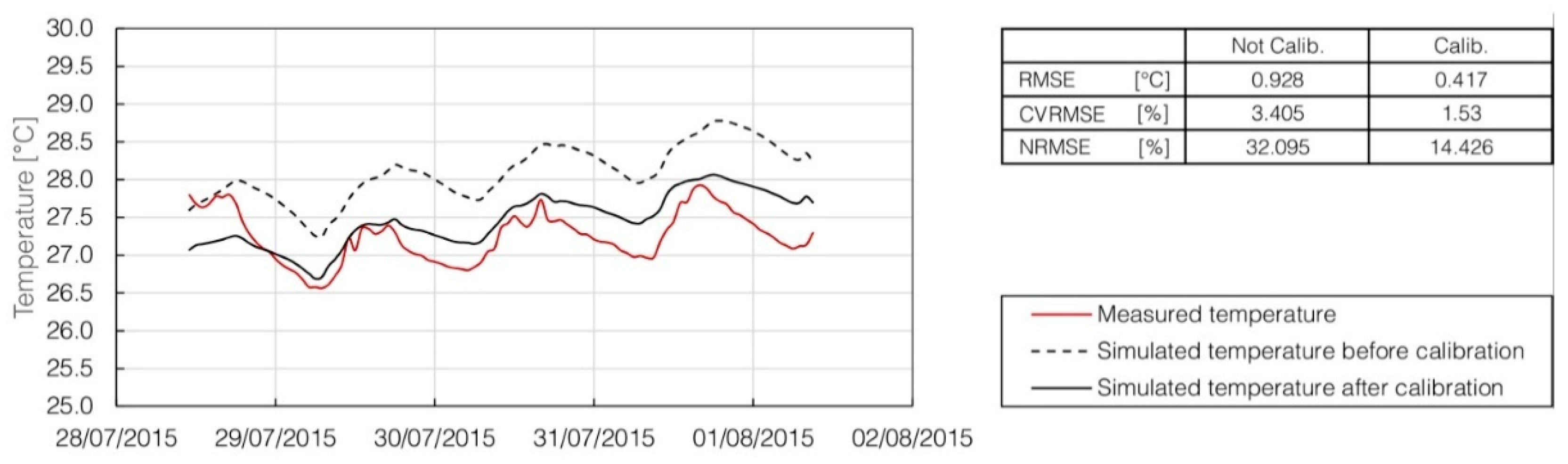
The second calibration process was directed again to the building envelope but concentrating on the basement floor. Calibration B involved parameters related to external wall with tuff cladding and external wall with marble cladding (layers), new windows (glass thermal transmittance) and their integrated shading (multiplier for solar gain). Details are reported in

Table 7. Parameters collection for Calibration B *.

Reference	Element	First Guess	Lower Bound	Upper Bound
Ext. Wall-Marble	s Int. Brick [m]	0.12	0.08	0.12
	s Air [m]	0.04	0.04	0.08
	s Ext. Brick [m]	0.08	0.08	0.12
Ext. Wall-Tuff	s Int. Brick [m]	0.12	0.08	0.12
	s Air [m]	0.04	0.03	0.05
Shading (refurbished windows)	mult. g	0.15	0.15	0.4
	mult. U	0.9	0.8	1
	D	1	0.5	1
Windows (refurbished)	U	2.6	1.1	2.6

* s = thickness, mult. g = multiplier for glass solar gain, mult. U = multiplier for glass thermal transmittance, D = diffusion factor, g = glass solar gain, U = glass thermal transmittance.

.

The calibration required almost 2 weeks to achieve the final solution (Figure 9). In the figure, only the most representative simulations needed (25) are shown (where the run of each simulation took 4–5 min to be completed).

3.1.3. Calibration C (Heating System)

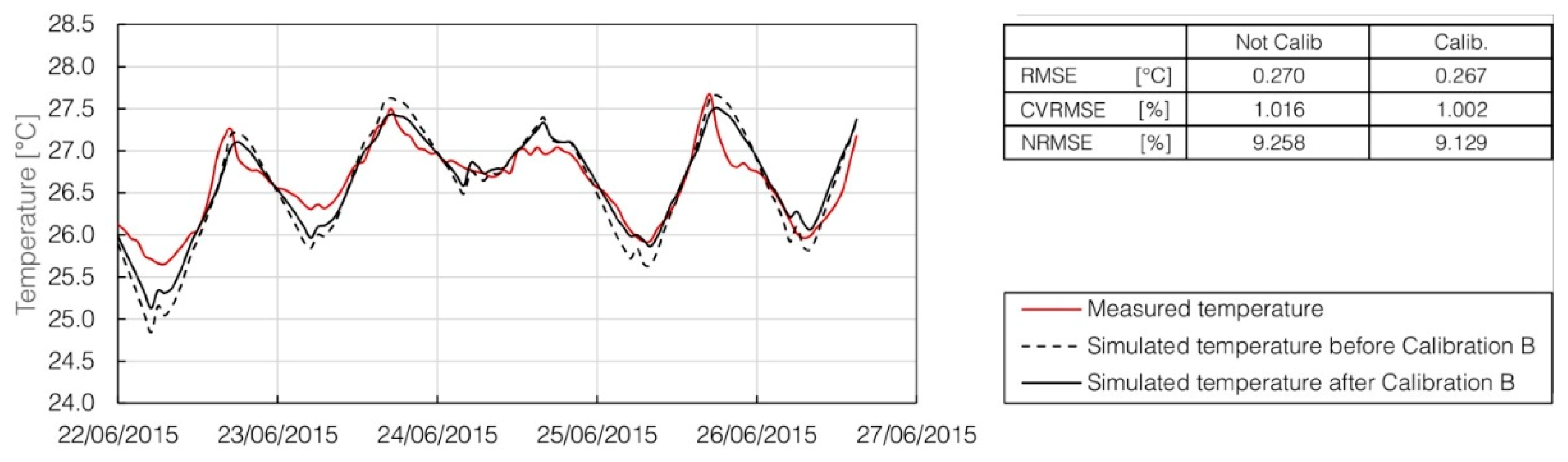
The tuning objective for Calibration C was the heating system. Since the first guess model simulated a lower temperature than measured (almost constant difference of 1 °C), the water radiator’s emitted power was considered the main element to be involved for this tuning process. Parameters related to emitted power equation as exponent N (Equation (11)) and maximum emitted power at capacity equation from UNI10200 as experimental parameter C (Equation (12)) were then considered (

Table 8. Parameters collection for Calibration C.

Reference	Element	First Guess	Lower Bound	Upper Bound
Radiators	Exponent N	1.28	1.28	1.33
	Parameter C	22,500	22,500	28,100

).

The calibration needed about 3 weeks to achieve the final solution and 15 simulations (where the run of each simulation took 10–12 min to be completed) are shown in Figure 10.

3.2. Automatic Calibration

3.2.1. Calibration A (First Floor)

Initially, k = 33 parameters, involving thermal bridges, infiltration, walls’ layers, emissivity and reflectance, windows and shading properties, were considered (details reported in

Table 9. Parameters collection for Sensitivity Analysis A *.

Reference	Element	First Guess	Lower Bound	Upper Bound
Linear Transmittance of Thermal Bridges	Ext. Wall-Int.l Wall [W/(K⋅m)]	0.03	0.024	0.036
	Ext. Wall-Ext. Wall [W/(K⋅m)]	0.08	0.064	0.096
	Window Perimeter [W/(K⋅m)]	0.03	0.024	0.036
	Door Perimeter [W/(K⋅m)]	0.03	0.024	0.036
	Ext. Wall-Roof [W/(K⋅m)]	0.09	0.072	0.102
	Int.Wall-Roof [W/(K⋅m)]	0.03	0.024	0.036
Infiltration	ACH	0.5	0.4	0.6
Ext. Wall -Brick	s Int. Brick [m]	0.12	0.1	0.14
	s Air [m]	0.04	0.03	0.05
	s Ext. Brick [m]	0.12	0.1	0.14
	E Ext. Surface	0.9	0.72	1
	R Ext. Surf	0.5	0.4	0.6
Ext. Wall-Marble	s Int. Brick [m]	0.12	0.1	0.14
	s Air [m]	0.04	0.03	0.05
	s Ext. Brick [m]	0.08	0.06	0.1
	E Ext. Surface	0.9	0.72	1
	R Ext. Surf	0.5	0.4	0.6
Ext. Wall-Tuff	s Int. Brick [m]	0.12	0.1	0.14
	s Air [m]	0.04	0.03	0.05
	E Ext. Surface	0.9	0.72	1
	R Ext. Surf	0.5	0.4	0.6
Roof	s Screed [m]	0.07	0.05	0.09
	s Air [m]	0.04	0.03	0.05
	s Slab [m]	0.04	0.03	0.05
	s Joist [m]	0.16	0.12	0.2
	E Ext. Surface	0.9	0.72	1
	R Ext. Surf	0.5	0.4	0.6
Material Properties	λ Brick [W/(m⋅K)]	0.387	0.3096	0.4644
	λ Concrete [W/(m⋅K)]	1.23	0.984	1.476
	λ Str. Concrete [W/(m⋅K)]	1.91	1.528	2.292
	λ Concrete-Brick [W/(m⋅K)]	0.6	0.48	0.72
Shading (original windows)	mult. g	0.15	0.12	0.18
	mult. U	0.9	0.72	1

* s = thickness, E = emissivity, R = reflectance, λ = thermal conductivity, mult. g = multiplier for glass solar gain, mult. U = multiplier for glass thermal transmittance.

).

Subsequently, considering for each parameter a number of EEs r = 10, a number of discretized levels L = 6 to search in a fixed uncertainty range of ±20% from first guessed value, SA was performed and, after 17 h of computational time, the number of parameters was reduced to 10 (Figure 11).

The input parameters were then selected, and it was possible to set and run the optimization problem for the calibration. Once started, the optimization needed 437 simulations and about 5 h of total computation time to achieve the final solution (Figure 12).

3.2.2. Calibration B (Basement)

Using the final result of the first stage as new initial model, in this second phase again k = 17 parameters were considered (details reported in

Table 10. Parameters collection for Sensitivity Analysis B *.

Reference	Element	First Guess	Lower Bound	Upper Bound
Ext. Wall-Brick	s Int. Brick [m]	0.12	0.1	0.14
	s Air [m]	0.04	0.03	0.05
	s Ext. Brick [m]	0.12	0.1	0.14
Ext. Wall-Marble	s Int. Brick [m]	0.12	0.1	0.14
	s Air [m]	0.04	0.03	0.05
	s Ext. Brick [m]	0.08	0.06	0.1
	E Ext. Surface	0.9	0.72	1
	R Ext. Surf	0.5	0.4	0.6
Ext. Wall-Tuff	s Int. Brick [m]	0.12	0.1	0.14
	s Air [m]	0.04	0.03	0.05
	E Ext. Surface	0.9	0.72	1
	R Ext. Surf	0.5	0.4	0.6
Material Properties	λ Tuff [W/(m⋅K)]	0.55	0.44	0.66
	λ Soil [W/(m⋅K)]	1.23	0.984	1.476
Shading (refurbished windows)	mult. G	0.15	0.12	0.18
	mult. U	0.9	0.72	1
Soil	s Soil [m]	2	1.6	2.4

* s = thickness, E = emissivity, R = reflectance, λ = thermal conductivity, mult. g = multiplier for glass solar gain, mult. U = multiplier for glass thermal transmittance.

).

Taking into account the identical settings of the previous case (number of EEs r = 10, number of levels L = 6 and fixed uncertainty range of ±20% from initial value), SA was performed and, after 9 h of computational time, the number of parameters was reduced to 9 (Figure 13).

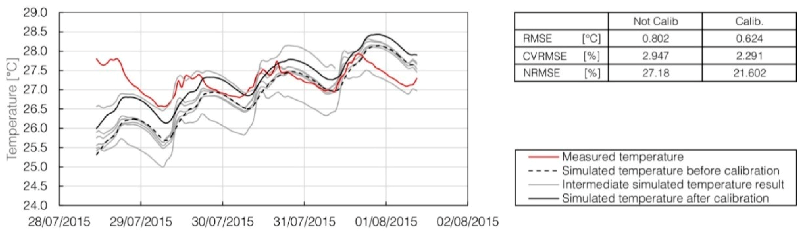
The selected input parameters were involved in the second optimization problem for the calibration. Once started, the optimization needed 408 simulations and about 4.5 h of total computation time to achieve the final solution (Figure 14).

Calibration B included envelope-related parameters. Referring to the first calibration period and monitoring the simulated T in the office room used for Calibration A, a check simulation has been done to evaluate the effect on the previous results of the changes introduced in the above-mentioned parameters. This comparison results in a cross validation since the calibrated model output were compared with experimental data coming from a different time period and a different zone of the building. Not only was the effect restrained but also positive in terms of accuracy of the model (Figure 15).

3.2.3. Calibration C (Heating System)

Starting from the result of the second stage as the new initial model, in this third phase the envelope of the model was considered as calibrated and the tuning process focused on the plant.

As the most of plant-related parameters were known or deducible and, conversely to the manual calibration case, changes on emitted power equation parameters were not giving sensitive model improvements, the highest uncertainty was considered to be related to the controller for supply heating water temperature.

A first calibration attempt was done trying to individuate the most appropriate heating curve. Although the statistics parameters for temperature were good for the model resulting by this calibration process, the validation was not confirming the goodness of the process. Although the whole year consumption was similar for real building and energy model, the monthly amount of gas consumed resulted to be strongly higher for warmer periods (1–27 November 2014 and 13 March–14 April 2015) and lower for the colder one (24 December 2014–22 January 2015), which resulted in a too high CVRMSE value. A new strategy was then adopted.

Referring to real fuel consumption from the bills (Table 2), it was possible to notice that, despite the change in the outdoor conditions in the passing months, the amount of consumed gas did not present relevant variations. This suggested an almost constant trend for the supply heating water temperature, which could be justified, assuming that, due to the long duration of service, the controller is not working properly anymore.

According to this new hypothesis, a second and definitive attempt was done to calibrate the plant system.

Since the number of parameters pre-selected (

Table 11. Parameters collection for Calibration C.

Reference	Element	First Guess	Lower Bound	Upper Bound
Controller for supply heating water temperature	Water T at ambient T = −30 °C [°C]	45	45	55
	Water T at ambient T = 30 °C [°C]	45	45	55
Radiators emitted power	Exponent N	1.28	1.26	1.30
Internal gains	Equipment power [W]	100	100	200

) was restricted (k = 4) no SA was performed in this case.

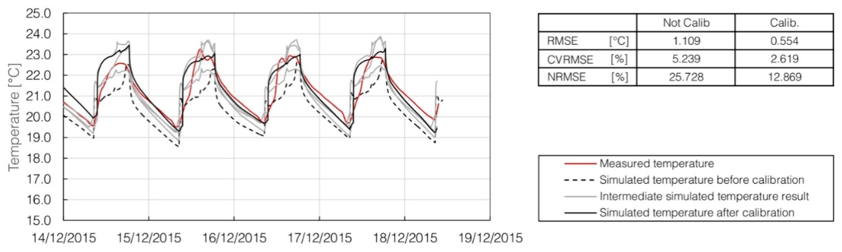
Involving these input parameters, the third optimization problem for the calibration was settled and run. Once started the optimization needed 299 simulations and about 6 h of total computation time to achieve the final solution (Figure 16).

4. Discussion

Table 12. Infiltration and thermal bridges input for resulting model from manual and automatic calibration (bold when changed).

Infiltrations
Element	Method		Air Tightness [ACH]
Wind driven flow	Manual		0.5
	Automatic		0.5
Thermal Bridges
Element 1	Element 2	Method	Thermal bridge [W/mK]
External wall	Internal wall	Manual	0.03
		Automatic	0.03
External wall	External wall	Manual	0.08
		Automatic	0.08
External windows perimeter	-	Manual	0.03
		Automatic	0.03
External doors perimeter	-	Manual	0.03
		Automatic	0.03
Roof	External wall	Manual	0.09
		Automatic	0.09
Roof	Internal wall	Manual	0.03
		Automatic	0.03

,

Table 13. Plants and internal gains settings for resulting models from manual and automatic calibration (bold when changed).

Controller three-ways valve
Element	Method			Temperature [°C]
Air 1	Manual			−26.0
	Automatic			−30.0
Air 2	Manual			20.0
	Automatic			30.0
Water 1	Manual			70.0
	Automatic			50.0
Water 2	Manual			20.0
	Automatic			47.0
Radiators
Element	Method	q [W]	C [W/m2⋅K]	N
Refurbished radiators	Manual	147.4	-	1.339
	Automatic	147.4	-	1.339
Original radiators	Manual	-	28,100	1.330
	Automatic	-	22,500	1.285
Internal gains
Element	Mehtod			Equipment power [W]
Equipment	Manual			100.0
	Automatic			188.8

and

Table 14. Construction elements for resulting models from manual and automatic calibration (bold when changed).

Doors
Element	Method	s [cm]				Layer 1
Internal door	Manual	5				Wood
	Automatic	5				Wood
External door	Manual	7				Wood
	Automatic	7				Wood
Internal Shading
Element	Method	Multiplier ${\mathrm{U}}_{\mathrm{glass}}$		Multiplier ${\mathrm{g}}_{\mathrm{glass}}$		Multiplier T		Diffusion factor
Refurbished roller blind	Manual	0.9		0.4		0.09		0.5
	Automatic	0.9		0.12		0.09		1
Original roller blind	Manual	0.8		0.2		0.09		0.5
	Automatic	0.7		0.17		0.09		1
Slabs
Element	Method	s [cm]	Layer 1	Layer 2	Layer 3	Layer 4	Layer 5	Layer 5	U [W/m2K]
Basement floor	Manual	54.5	Gravel (40 cm)	Concrete (13 cm)	Gres (1.5 cm)	-	-	-	1.615
	Automatic	54.5	Gravel (40 cm)	Concrete (13 cm)	Gres (1.5 cm)	-	-	-	1.615
Internal floor	Manual	22.5	Plaster (1 cm)	Joist (12 cm)	Slab (4 cm)	Concrete (4 cm)	Gres (1.5 cm)	-	2.238
	Automatic	22.5	Plaster (1 cm)	Joist (12 cm)	Slab (4 cm)	Concrete (4 cm)	Gres (1.5 cm)	-	2.238
Roof	Manual	43	Plaster (1 cm)	Joist (24 cm)	Slab (4 cm)	Air (4cm)	Concrete (9 cm)	Bitouminos membrane (1 cm)	1.337
	Automatic	30	Plaster (1 cm)	Joist (12 cm)	Slab (4 cm)	Air (4cm)	Concrete (7 cm)	Bitouminos membrane (1 cm)	1.325
Surfaces
Element	Method	Emissivity				Reflectance
External wall brick cladding	Manual	0.90				0.50
	Automatic	0.95				0.56
External wall marble cladding	Manual	0.90				0.50
	Automatic	0.96				0.50
External wall tuff cladding	Manual	0.90				0.50
	Automatic	0.96				0.60
Roof	Manual	0.90				0.50
	Automatic	0.80				0.45
Walls
Element	Method	s [cm]	Layer 1	Layer 2		Layer 3	Layer 4	Layer 5	U [W/m2K]
External wall brick cladding	Manual	30	Plaster (2 cm)	Brick (12 cm)		Air (4 cm)	Brick (12 cm)		1.005
	Automatic	30	Plaster (2 cm)	Brick (12 cm)		Air (4 cm)	Brick (12 cm)		0.834
External wall marble cladding	Manual	34	Plaster (2 cm)	Brick (12 cm)		Air (4 cm)	Brick (8 cm)	Marble (4 cm)	1.041
	Automatic	34	Plaster (2 cm)	Brick (12 cm)		Air (4 cm)	Brick (8 cm)	Marble (4 cm)	0.824
External wall tuff cladding	Manual	30	Plaster (2 cm)	Brick (12 cm)		Air (4 cm)	Tuff (12 cm)		1.043
	Automatic	36	Plaster (2 cm)	Brick (16 cm)		Air (6 cm)	Tuff (12 cm)		0.792
Windows
Element	Method	${\mathrm{U}}_{\mathrm{glass}}$ [W/m2K]	${\mathrm{U}}_{\mathrm{frame}}$ [W/m2K]	${\mathrm{g}}_{\mathrm{glass}}$		T	Internal shading
Refurbished Window	Manual	1.1	2	0.39		0.31	Refurbished roller blind
	Automatic	2.6	2	0.39		0.31	Refurbished roller blind
Original Window	Manual	5.8	3	0.59		0.48	Original roller blind
	Automatic	5.8	3	0.59		0.48	Original roller blind
Glazed doors	Manual	5.8	5.2	0.59		0.48	-
	Automatic	5.8	5.2	0.59		0.48	-

show final model settings for both manual and automatic procedure. Table 12 presents infiltration and thermal bridges values that were not modified during both calibration processes.

Table 13 and Table 14 show the values of the parameters obtained during manual and automatic calibration, where bold values indicate those parameters modified during the processes.

Concerning the construction elements’ parameters, the manually calibrated model presented higher thickness for roof slab (0.24 m vs. 0.12 m), while the automatic model shows lower values for roof surface emissivity and reflectance (0.80 and 0.45 vs. 0.90 and 0.50) and for λ-value of brick materials (0.312 W/mK vs. 0.387 W/mK). Those discordant values are different attempts to increase simulated T from first guess model in Calibration A. In addition, the manual model presents higher values for ${\mathrm{U}}_{\mathrm{glass}}$ and ${\mathrm{g}}_{\mathrm{glass}}$ multiplier for both original (0.90 and 0.40 vs. 0.90 and 0.12) and refurbished (0.80 and 0.20 vs. 0.70 and 0.17) internal shading, while the automatically calibrated model shows higher U-value for refurbished windows (2.6 W/m²K vs. 1.1 W/m²K), emissivity and reflectance surface parameters of brick wall (0.95 and 0.56 vs. 0.90 and 0.50) and marble wall (0.96 and 0.50 vs. 0.90 and 0.50) and for tuff wall thickness (0.16 m vs. 0.12 m).

Different results and configurations in Calibration A lead to a different starting model for Calibration B—if the manual model resulted in simulating a lower temperature than measured, the automatic model, in reverse, provided a higher value of indoor T. Calibrations then attempted to rise internal T (increasing solar gain and insulation) or decrease it (through emissivity, reflectance and wall thickness) for manual and automatic procedures, respectively.

Concerning the plants’ related parameters, the manual model keeps a standard heating curve which gives lower mean supply water T values but higher emitted power for radiators. The automatic model instead has an almost constant value for supply water T and radiator parameters obtained as standard from UNI 10200. The two approaches attempted to increase simulated indoor T for the manual procedure or to adjust indoor T value while keeping almost constant fuel consumption, for the automatic procedure.

Nevertheless, both methods show good and physically plausible results in having representative models for the case study.

Comparing results from both methods (

Table 15. Multi-stage calibration results comparison for manual and automatic methods. In bold the best results.

Calibration	Calibration A		Calibration B		Calibration C
Period	21 June 2015–26 June 2015		28 July 2015–1 August 2015		13 December 2015–18December 2015
Method	Manual	Automatic	Manual	Automatic	Manual	Automatic
Time	1 [mon]	17 (SA) + 5 [h]	2 [week]	9 (SA) + 4.5 [h]	3 [week]	0 (SA) + 6 [h]
Simulations	51	340 (SA) + 437	25	180 (SA) + 408	15	0 (SA) + 299
RMSE	0.350	0.270	0.624	0.417	0.554	0.390
CVRMSE	1.315	1.016	2.291	1.530	2.619	1.844
NRMSE	11.980	9.258	21.602	14.426	12.869	9.058

), it is possible to observe how automatic calibration (in bold) leads to better solutions in terms of statistical parameters (in every stage of the tuning process). In addition, the time needed to achieve the above-mentioned results (even including SA, when applied) is strongly reduced through automation, which also allows the evaluation of a higher number of scenarios.

Comparison with the Energy Bills

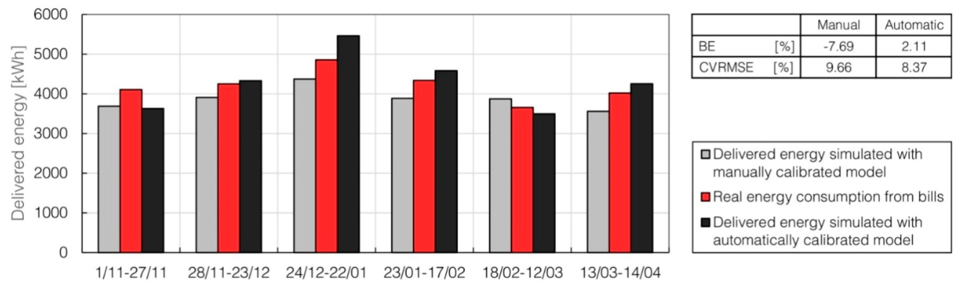
Data related to the heating system consumption of the building and the manual and automatic calibrated models (MCM and ACM, respectively) were compared (both monthly and seasonally) in order to assess the magnitude of the error made in terms of energy consumption, considering the relative Bias Error (BE) and CVRMSE.

The climate file used for the energy simulation for the period of interest was built through data coming from the ESTER lab, University of Rome Tor Vergata, Rome, Italy.

The fuel heating consumption comparison for MCM (

Table 16. Monthly and seasonal heating fuel consumption as measured from bills and as simulated with MCM.

Period	Measured Heating Fuel [scm]	Measured Primary Energy [kWh]	Simulated Primary Energy [kWh]	BE [%]	MBE [%]	CVRMSE [%]
1–27 November 2014	373	4107	3687	−10.23	-	-
28 November–23 December 2014	386	4250	3909	−8.03	-	-
24 December 2014–22 January 2015	441	4856	4374	−9.92	-	-
23 January–17 February 2015	394	4338	3885	−10.45	-	-
18 February–12 March 2015	332	3656	3872	5.92	-	-
13 March–14 April 2015	365	4019	3559	−11.45	-	-
1 November 2014–14 April 2015	2291	25,226	23,286	-	−7.69	9.69

) showed a good monthly value for BE, barely higher (in absolute value) than 10%. Global value for BE exceeded the limits fixed by ASHRAE guideline but CVRMSE was optimal.

The fuel heating consumption comparison for ACM is shown in

Table 17. Monthly and seasonal heating fuel consumption as measured from bills and as simulated with ACM.

Period	Measured Heating Fuel [scm]	Measured Primary Energy [kWh]	Simulated Primary Energy [kWh]	BE [%]	MBE [%]	CVRMSE [%]
1–27 November 2014	373	4107	3631	−11.59	-	-
28 November–23 December 2014	386	4250	4330	1.88	-	-
24 December 2014–22 January 2015	441	4856	5464	12.52	-	-
23 January–17 February 2015	394	4338	4582	5.62	-	-
18 February–12 March 2015	332	3656	3497	−4.34	-	-
13 March–14 April 2015	365	4019	4254	5.85	-	-
1 November 2014–14 April 2015	2291	25,226	25,758	-	2.11	8.37

. As predicted, the consumption period related to the same part of the year of the calibration week showed best result. Worse but still acceptable results were obtained for the warmer periods (1–27 November 2014 and 13 March–14 April 2015), as well as for the colder one (24 December 2014–22 January 2015). Global values for BE and CVRMSE were optimal according to the bounds fixed by the ASHRAE guideline. Little disagreement between simulated and real data could be explained by the fact that primary energy consumption was estimated and not directly measured by the gas company.

Energy consumption comparison between MCM, ACM and real bills (Figure 17 and Figure 18) shows that MCM generally underestimates the energy consumption (only period 18 February–12 March has a higher value for simulated energy, at 5.92%) with an almost constant BE value (around −10%).

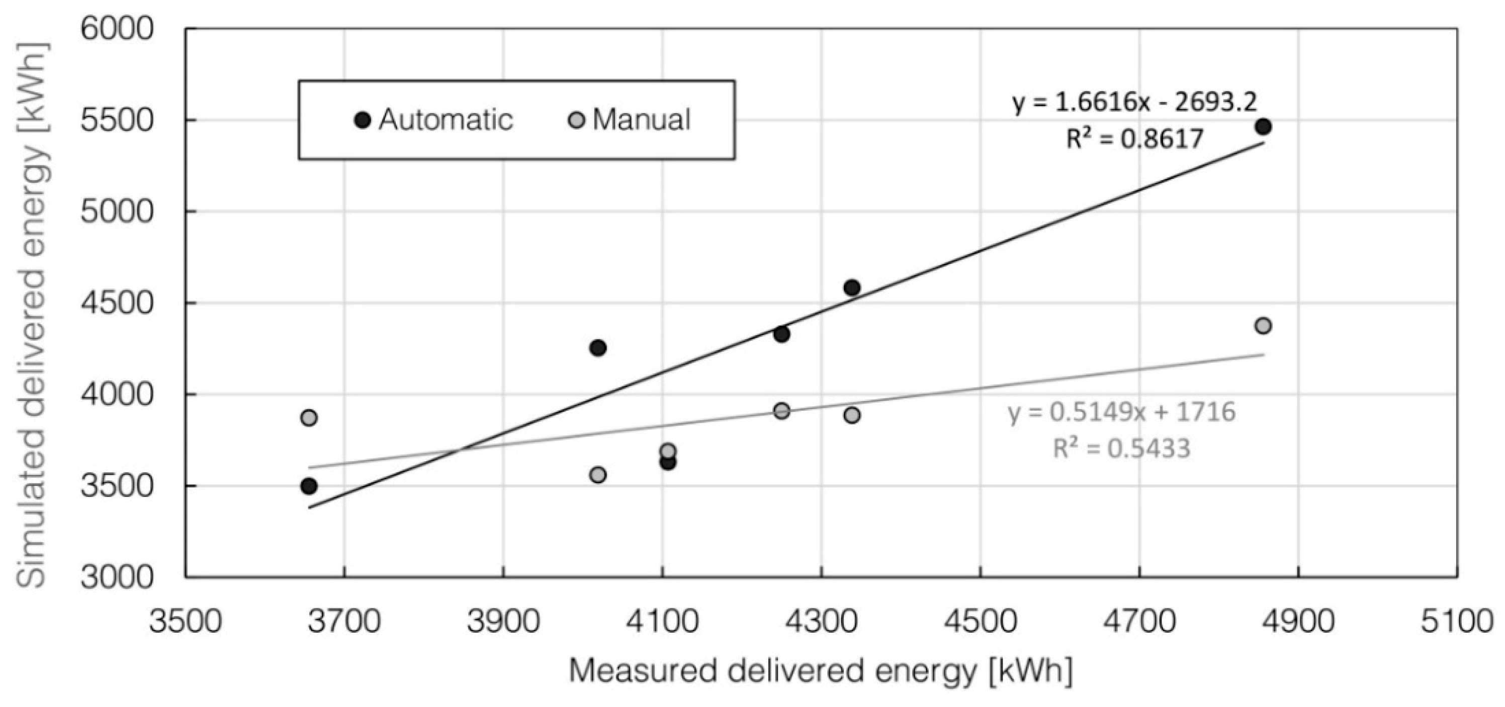
This leads to a lower simulated seasonal consumption, probably due to the insufficient water supply T of the standard heating curve, not completely suitable with the improvements on radiators’ power emission. On the other hand, ACM does not show a constant trend, generally overestimating colder periods and underestimating warmer ones. This leads to a more equilibrated seasonal BE value, which globally lightly overestimates energy consumption. In addition, even if the BE for 1–27 November and 24 December–22 January results are worse for the automatic calibration, other periods’ consumption is definitely more accurate, resulting in a lower CVRMSE value. So, for this specific case, ACM better fits the real energy consumption than MCM. This conclusion could imply that ACM could provide a more reliable prediction of energy consumption than MCM in cases in which the energy model would be used for evaluating the energy performance of building retrofit solutions.

5. Conclusions

The work presented introduces an automatic calibration procedure and compares it against a manual process to evidence differences, advantages and disadvantages by applying both of them to a dynamic simulation model of a real office building in Rome. The methodology for automatic calibration includes SA for selecting the most relevant parameters and simulation-based optimization to minimize the difference between the simulated and measured data, automatically performed coupling of IDA ICE and MatLab and IDA ICE and GenOpt, respectively. It has to be considered that the main calibration activity was pre-eminently focused on the envelope, in some part on the plant and marginally on the equipment. Although occupancy and lightning could be generally relevant for calibration procedures, they were not considered in this analysis since they were not influential in this particular study. So, in principle, the results of this paper could be considered valid for cases in which these parameters can be neglected. Both manual and automatic calibrations show good results in terms of accuracy and a physically plausible representation of the case study, although automation presents finer tuning results, even in a reduced time frame. For instance, referring to the envelope calibration, the manual procedure gave an RMSE of 0.35 °C and 0.62 °C for calibration A (first floor) and calibration B (basement) respectively, while results for the automatic procedure showed an RMSE of 0.27 °C and 0.42 °C. Concerning heating system calibration, an RMSE of 0.54 °C and 0.39 °C resulted respectively from manual and automatic processes. Automatic calibration results in a better prediction of energy consumption since the comparison with real consumption bills produces a BE of 2.11% and a CVRMSE of 8.37% versus a BE of −7.69% and a CVRMSE of 9.66% for the manual process. Nevertheless, automatic calibration appears still strictly linked to the operator expertise, since the quality of the results depends on the settings and monitoring of the optimization procedure.

References

- D’Agostino, D.; Cuniberti, B.; Bertoldi, P. Energy consumption and efficiency technology measures in European non-residential buildings. Energy Build. 2017, 153, 72–86. [Google Scholar] [CrossRef]
- Allouhi, A.; El Fouih, Y.; Kousksou, T.; Jamil, A.; Zeraouli, Y.; Mourad, Y. Energy consumption and efficiency in buildings: Current status and future trends. J. Clean. Prod. 2015, 109, 118–130. [Google Scholar] [CrossRef]
- Li, B.; Yao, R. Urbanisation and its impact on building energy consumption and efficiency in China. Renew. Energy 2009, 34, 1994–1998. [Google Scholar] [CrossRef]
- Hong, T.; Yang, L.; Hill, D.; Feng, W. Data and analytics to inform energy retrofit of high performance buildings. Appl. Energy 2014, 126, 90–106. [Google Scholar] [CrossRef] [Green Version]
- Klein, S.A.; Beckman, W.A.; Mitchell, J.W.; Duffie, J.A.; Duffie, N.A.; Freeman, T.L.; Mitchell, J.C.; Braun, J.E.; Evans, B.L.; Kummer, J.P.; et al. TRNSYS 17 Manual: A TRaNsient SYstem Simulation Program, Solar Energy Laboratory. 2012. Available online: http://sel.me.wisc.edu/trnsys.No 2012 (accessed on 10 November 2014).
- Crawley, D.B.; Lawrie, L.K.; Winkelmann, F.C.; Buhl, W.F.; Huang, Y.J.; Pedersen, C.O.; Strand, R.K.; Liesen, R.J.; Fisher, D.E.; Witte, M.J.; et al. EnergyPlus: Creating a new-generation building energy simulation program. Energy Build. 2001, 33, 319–331. [Google Scholar] [CrossRef]
- Winkelmann, F.C.; Birdsall, B.E.; Buhl, W.F.; Ellington, K.L.; Erdem, A.E.; Hirsch, J.J.; Gates, S.D. DOE-2 Supplement: Version 2.1 E; No. LBL-34947; DOE: Oak Ridge, TN, USA, 1993.
- ESRU. E.S.R.U. ESP-r 1974; University of Strathclyde Energy Systems Research Unit: Glasgow, UK.
- Björsell, N.; Bring, A.; Eriksson, L.; Grozman, P.; Lindgren, M.; Sahlin, P.; Sha-povalov, A.; Vuolle, M. IDA Indoor climate and energy. In Proceedings of the Building Simulation Conference, Kyoto, Japan, 13–15 September 1999. [Google Scholar]
- Crawley, D.B.; Hand, J.W.; Kummert, M.; Griffith, B.T. Contrasting the capabilities of building energy performance simulation programs. Build. Environ. 2008, 43, 661–673. [Google Scholar] [CrossRef] [Green Version]
- Royapoor, M.; Roskilly, T. Building model calibration using energy and environmental data. Energy Build. 2015, 94, 109–120. [Google Scholar] [CrossRef] [Green Version]
- Ascione, F.; Bianco, N.; De Stasio, C.; Mauro, G.M.; Vanoli, G.P. Energy retrofit of educational buildings: Transient energy simulations, model calibration and multi-objective optimization towards nearly zero-energy performance. Energy Build. 2017, 144, 303–319. [Google Scholar] [CrossRef]
- Yang, T.; Pan, Y.; Mao, J.; Wang, Y.; Huang, Z. An automated optimization method for calibrating building energy simulation models with measured data: Orientation and a case study. Appl. Energy 2016, 179, 1220–1231. [Google Scholar] [CrossRef]
- Robertson, J.J.; Polly, B.J.; Collis, J.M. Reduced-order modeling and simulated annealing optimization for efficient residential building utility bill calibration. Appl. Energy 2015, 148, 169–177. [Google Scholar] [CrossRef] [Green Version]
- Roberti, F.; Oberegger, U.F.; Gasparella, A. Calibrating historic building energy models to hourly indoor air and surface temperatures: Methodology and case study. Energy Build. 2015, 108, 236–243. [Google Scholar] [CrossRef] [Green Version]
- Penna, P.; Cappelletti, F.; Gasparella, A.; Tahmasebi, F.; Mahdavi, A. Multi-Stage Calibration of the Simulation Model of a School Building Through Short-Term Monitoring. J. Inf. Technol. Constr. 2015, 20, 132–145. [Google Scholar]
- ASHRAE Guideline 14-2002: Measurement of Energy and Demand Savings; ASHRAE: Atlanta, GA, USA, 2002.
- Specialists, E.E.V. International Performance Measurement and Verification Protocol (IPMVP); DOE: Oak Ridge, TN, USA, 2002.
- United States Department of Energy. M&V Guidelines: Measurement and Verification for Federal Energy Projects Version 3.0; DOE: Oak Ridge, TN, USA, 2008.
- Coakley, D.; Raftery, P.; Keane, M. A review of methods to match building energy simulation models to measured data. Renew. Sustain. Energy Rev. 2014, 37, 123–141. [Google Scholar] [CrossRef]
- Fumo, N. A review on the basics of building energy estimation. Renew. Sustain. Energy Rev. 2014, 31, 53–60. [Google Scholar] [CrossRef]
- Reddy, T.A. Literature review on calibration of building energy simulation programs: Uses, problems, procedures, uncertainty and tools. ASHRAE Trans. 2006, 112, 226–240. [Google Scholar]
- Coakley, D.; Raftery, P.; Molloy, P.; White, G. Calibration of a Detailed BES Model to Measured Data Using an Evidence-Based Analytical Optimisation Approach. In Proceedings of the Building Simulation, Sydney, Australia, 14–16 November 2011; pp. 374–381. [Google Scholar]
- Westphal, F.S.; Lamberts, R. Building Simulation Calibration Using Sensitivity Analysis. In Proceedings of the Ninth International IBPSA Conference, Montréal, QC, Canada, 15–18 August 2005; pp. 1331–1338. [Google Scholar]
- Pan, Y.; Huang, Z.; Wu, G. Calibrated building energy simulation and its application in a high-rise commercial building in Shanghai. Energy Build. 2007, 39, 651–657. [Google Scholar] [CrossRef]
- Raftery, P.; Keane, M.; O’Donnell, J. Calibrating whole building energy models: An evidence-based methodology. Energy Build. 2011, 43, 2356–2364. [Google Scholar] [CrossRef]
- Pedrini, A.; Westphal, F.S.; Lamberts, R. A methodology for building energy modelling and calibration in warm climates. Build. Environ. 2002, 37, 903–912. [Google Scholar] [CrossRef] [Green Version]
- Mustafaraj, G.; Marini, D.; Costa, A.; Keane, M. Model calibration for building energy efficiency simulation. Appl. Energy 2014, 130, 72–85. [Google Scholar] [CrossRef]
- Cornaro, C.; Puggioni, V.A.; Strollo, R.M. Dynamic simulation and on-site measurements for energy retrofit of complex historic buildings: Villa Mondragone case study. J. Build. Eng. 2016, 6, 17–28. [Google Scholar] [CrossRef]
- Frasca, F.; Siani, A.; Cornaro, C. On-site measurements and whole-building thermal dynamic simulation of a semi-confined prefabricated building for heritage conservation. In Proceedings of the BSA 2017—Building Simulation Applications 3rd IBPSA-Italy Conference, Bozen-Bolzano, Italy, 8–10 February 2017. [Google Scholar]
- Lomas, K.J.; Eppel, H. Sensitivity analysis techniques for building thermal simulation programs. Energy Build. 1992, 19, 21–44. [Google Scholar] [CrossRef]
- O’Neill, Z.; Eisenhower, B. Leveraging the analysis of parametric uncertainty for building energy model calibration. Build. Simul. 2013, 6, 365–377. [Google Scholar] [CrossRef]
- Heo, Y.; Choudhary, R.; Augenbroe, G.A. Calibration of building energy models for retrofit analysis under uncertainty. Energy Build. 2012, 47, 550–560. [Google Scholar] [CrossRef]
- Sun, K.; Hong, T.; Taylor-Lange, S.C.; Piette, M.A. A pattern-based automated approach to building energy model calibration. Appl. Energy 2016, 165, 214–224. [Google Scholar] [CrossRef] [Green Version]
- Hong, T.; Kim, J.; Jeong, J.; Lee, M.; Ji, C. Automatic calibration model of a building energy simulation using optimization algorithm. Energy Procedia 2017, 105, 3698–3704. [Google Scholar] [CrossRef]
- Lara, R.A.; Naboni, E.; Pernigotto, G.; Cappelletti, F.; Zhang, Y.; Barzon, F.; Gasparella, A.; Romagnoni, P. Optimization Tools for Building Energy Model Calibration. Energy Procedia 2017, 111, 1060–1069. [Google Scholar] [CrossRef]
- Penna, P.; Prada, A.; Cappelletti, F.; Gasparella, A. Multi-objectives optimization of Energy Efficiency Measures in existing buildings. Energy Build. 2015, 95, 57–69. [Google Scholar] [CrossRef]
- Chaudhary, G.; New, J.; Sanyal, J.; Im, P.; O’Neill, Z.; Garg, V. Evaluation of “Autotune” calibration against manual calibration of building energy models. Appl. Energy 2016, 182, 115–134. [Google Scholar] [CrossRef]
- Cacabelos, A.; Eguía, P.; Febrero, L.; Granada, E. Development of a new multi-stage building energy model calibration methodology and validation in a public library. Energy Build. 2017, 146, 182–199. [Google Scholar] [CrossRef]
- Morril, M.D.; Morris, M.A.X.D. Factorial Sampling Plans for Prelim inary Computational Experiments. Technometrics 1991, 33, 161–174. [Google Scholar] [CrossRef]
- Saltelli, A.; Tarantola, S.; Campolongo, F.; Ratto, M. Sensitivity Analysis in Practice: A Guide to Assessing Scientific Models; Wiley: Chichester, UK, 2004; p. 234. [Google Scholar]
- Taylor, K.E. Summarizing multiple aspects of model performance in a single diagram. J. Geophys. Res. 2001, 106, 7183–7192. [Google Scholar] [CrossRef] [Green Version]
- GenOpt Generic Optimization Program, 1998–2011; Lawrence Berkeley National Laboratory, University of California: Berkeley, CA, USA, 2015.
- Wetter, M. GenOpt—A Generic Optimization Program. In Proceedings of the Seventh International IBPSA Conference, Rio de Janeiro, Brazil, 13–15 August 2001; pp. 601–608. [Google Scholar]
- Kennedy, J. Particle Swarm Optimization. In Encyclopedia of Machine Learning; Springer: Boston, MA, USA, 2011; pp. 1942–1948. [Google Scholar]
- Karaboga, D.; Akay, B. A survey: Algorithms simulating bee swarm intelligence. Artif. Intell. Rev. 2009, 31, 61–85. [Google Scholar] [CrossRef]
- Kirgat, G.S.; Surde, A.N. Review of Hooke and Jeeves Direct Search Solution Method Analysis Applicable To Mechanical Design Engineering. Int. J. Innov. Eng. Res. Technol. 2014, 1, 1–14. [Google Scholar]
- CTI UNI 10200:2015—Impianti Termici Centralizzati di Climatizzazione Invernale e Produzione di Acqua Calda Sanitaria—Criteri di Ripartizione delle Spese di Climatizzazione Invernale ed Acqua Calda Sanitaria; Comitato Termotecnico Italiano: Milano, Italy, 2015.
Figure 1.
Methodology scheme.
Figure 2.
Coupling of a simulation program and an optimization engine in a simulation-based optimization method.
Figure 3.
The International Radio Medical Centre (CIRM) administrative headquarter building.
Figure 4.
Data acquired during the measurement campaigns. (a) data from survey A; (b) data from survey B; (c) data from survey C.
Figure 5.
First guess model in IDA-ICE’s 3D environment.
Figure 6.
Thermal zones. The highlighted zones refer to the rooms where the monitoring surveys were carried out.
Figure 7.
Heating plant scheme.
Figure 8.
Results for Calibration A. First floor, North exposure.
Figure 9.
Results for Calibration B. Basement, South exposure.
Figure 10.
Results from Calibration C. First floor, North-West exposure.
Figure 11.
Results for Sensitivity Analysis A. First floor, North exposure.
Figure 12.
Figure 13.
Results for Sensitivity Analysis B. Basement, South exposure.
Figure 14.
Figure 15.
Effect of Calibration B on the temperature trend of the first floor, North exposure.
Figure 16.
Results for Calibration C. First floor, North-West exposure.
Figure 17.
Delivered energy from manual and automatic calibrated models compared with real consumption from bills.
Figure 18.
Scatter plot of delivered energy from manual and automatic calibrated models compared with real consumption from bills.