Short-Term Load Forecasting for Electric Vehicle Charging Stations Based on Deep Learning Approaches


1
Industrial Technology Research Institute, Zhengzhou University, Zhengzhou 450001, China
2
Shenzhen Institute of Advanced Technology, Chinese Academy of Sciences, Shenzhen 518055, China
3
Winline Technology Co., Ltd., Shenzhen 518000, China
*
Author to whom correspondence should be addressed.
Appl. Sci. 2019, 9(9), 1723; https://doi.org/10.3390/app9091723
Submission received: 20 March 2019
/
Revised: 10 April 2019
/
Accepted: 15 April 2019
/
Published: 26 April 2019
(This article belongs to the Special Issue Energy Management and Smart Grids)
Abstract
:Short-term load forecasting is a key task to maintain the stable and effective operation of power systems, providing reasonable future load curve feeding to the unit commitment and economic load dispatch. In recent years, the boost of internal combustion engine (ICE) based vehicles leads to the fossil fuel shortage and environmental pollution, bringing significant contributions to the greenhouse gas emissions. One of the effective ways to solve problems is to use electric vehicles (EVs) to replace the ICE based vehicles. However, the mass rollout of EVs may cause severe problems to the power system due to the huge charging power and stochastic charging behaviors of the EVs drivers. The accurate model of EV charging load forecasting is, therefore, an emerging topic. In this paper, four featured deep learning approaches are employed and compared in forecasting the EVs charging load from the charging station perspective. Numerical results show that the gated recurrent units (GRU) model obtains the best performance on the hourly based historical data charging scenarios, and it, therefore, provides a useful tool of higher accuracy in terms of the hourly based short-term EVs load forecasting.
1. Introduction
Since the second industrial revolution, the steady supply of electricity load is a basic requirement for maintaining the normal functioning of modern society. Load forecasting can be divided into three categories on the basis time interval [1], long-term load forecast (1 year to 10 years ahead), medium-term load forecast (1 month to 1 year ahead), and short term load forecast (1 hour to 1 day or 1 week ahead). In recent years, the wide adoption of renewable energy has become an emerging pathway due to the shortage of fossil fuel such as petroleum, and the global warming due to the excessive carbon emissions [2]. One of the effective ways to solve the problem of fossil fuel shortage and environmental pollution is to popularize the electric vehicles (EVs) to replace traditional internal combustion engine (ICE) based vehicles. EVs are powered by electricity [3], which greatly reduces the consumption of petroleum resources and does not generate any environmentally polluting gases during the whole life cycles. With the fast development of the EV industry, it is bound to bring new changes to the power field due to the large capacity of the battery and stochastic charging behaviors of the users. In this regard, accurate short-term load forecasting is a key measure to the intelligent control of EV charging systems.
Power load forecasting models can be categorized into traditional statistical models and artificial intelligence models, traditional forecasting methods include time series method [4], autoregressive integrated moving average [5], regression analysis [6], Kalman filtering [7], etc. Artificial intelligence methods include artificial neural networks [8], support vector machines [9], and deep learning methods [10]. Before the 21st century, due to the strong adaptive, self-learning and generalization ability of artificial neural networks (ANN), it had become a hot research topic for adopting ANN approaches in load forecasting. The article [11] reviewed the application of ANNs for load forecasting and proved that ANNs have effectiveness for load forecasting in terms of accuracy and efficiency. In recent years, thanks to the breakthrough of computing hardware and successful applications such as Alpha-go, the deep learning methods have been obtained wide attractions and used in image semantic segmentation [12], image classification [13], target detection [14], natural language processing [15] and many other science and engineering fields. The network structure constructed by the deep learning methods is more complex with a large number of hidden layers and/or recurrent structure, which endowing stronger learning and self-adaptive ability than ANN methods. Therefore, attentions have also been paid in the field of load forecasting.
With the diversification of modern power grid systems, an increasing number of factors, including weather, holidays, real-time electricity prices, and even the degree of urban development and human being behaviors, have various impacts on load demand. Traditional load forecasting methods are unable to provide forecasting models with sufficient predictive accuracy. Therefore, deep learning methods are widely used in the field of load forecasting. Vermaak and Botha [16] used Recurrent neural networks (RNN) for the first time to establish a short-term load forecasting model. However, the conventional RNN would suffer from the gradient vanishing problem and the long short term memory (LSTM) network is an effective approach to relieve the issue. More recently, Marino et al. [17] proposed an LSTM architecture to forecast the load of individual residences [18]. Kong et al. [19] combined the energy consumption of a residence with the behavior of a resident, converted the behavior patterns of energy consumers into a sequence of input features to the network, thanks to which the accuracy of the load forecasting was improved. Some other studies [20,21,22,23] also used LSTM to load forecasting, whereas Lu et al. [24] used gated recurrent units and achieved more accurate results. Li, Y. et al. [25] used the niche immunity lion algorithm and Convolutional neural networks (CNN) for the one step short-term EVs charging load forecasting, where competitive forecasting accuracy could be obtained. Experimental results of these studies show that deep learning models have higher accuracy in load forecasting than the traditional methods.
Unlike normal industrial or household loads, EV loads are unique in both periodicity and fluctuation. The significant penetration of EVs would pose a large pressure to the power system particular the distributed network, which calls for more powerful tools for establishing accurate prediction models. In this paper, four deep learning models are preliminarily used to forecast EV charging station load, where real-world EV charging station datasets are adopted in the numerical study. The rest of the paper is organized as follow: Section 2 briefly describes three deep learning models; Section 3 introduces the dataset and proposes the data pre-processing method as well as load forecasting framework; the experimental results are shown in Section 4, followed by Section 5 concludes the paper and outlooks the future research.
2. Deep Learning Models
The concept of deep learning was proposed by Hinton et al. [10] in 2006, originated from the study of ANN. A multilayer perceptron with multiple hidden layers formulates a deep learning structure, combining low-level features to form more abstract high-level representation attribute categories or features and to discover distributed feature representations of data. Deep learning models have strong learning and generalization ability and would be competitive in complex forecasting tasks. This chapter nominates three structures of the recurrent neural network, aiming to investigate the comparative performance of the methods on the given EV load forecasting problem.
2.1. Recurrent Neural Networks
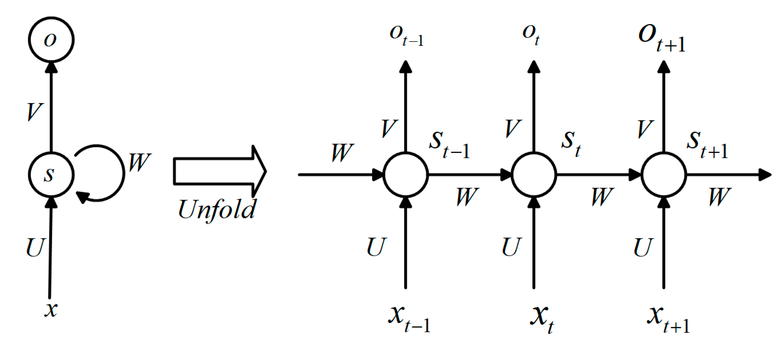
The load of EV charging is influenced by many factors including temperature, holiday, real-time electricity price, etc. These factors are difficult to quantify, resulting in low accuracy of the traditional model for EV charging station load forecasting. Thanks to the dynamic nature and instinctive structure, RNN models can better capture the characteristics of input data, whose structure is shown in Figure 1.
For time t:
where and denote the input and the hidden unit, while is the output at t. Moreover, V, W, U are network connection weights. In addition, b is bias, and is the model predicted output, is activation function, and tanh is well adapted as activation function shown as follows:
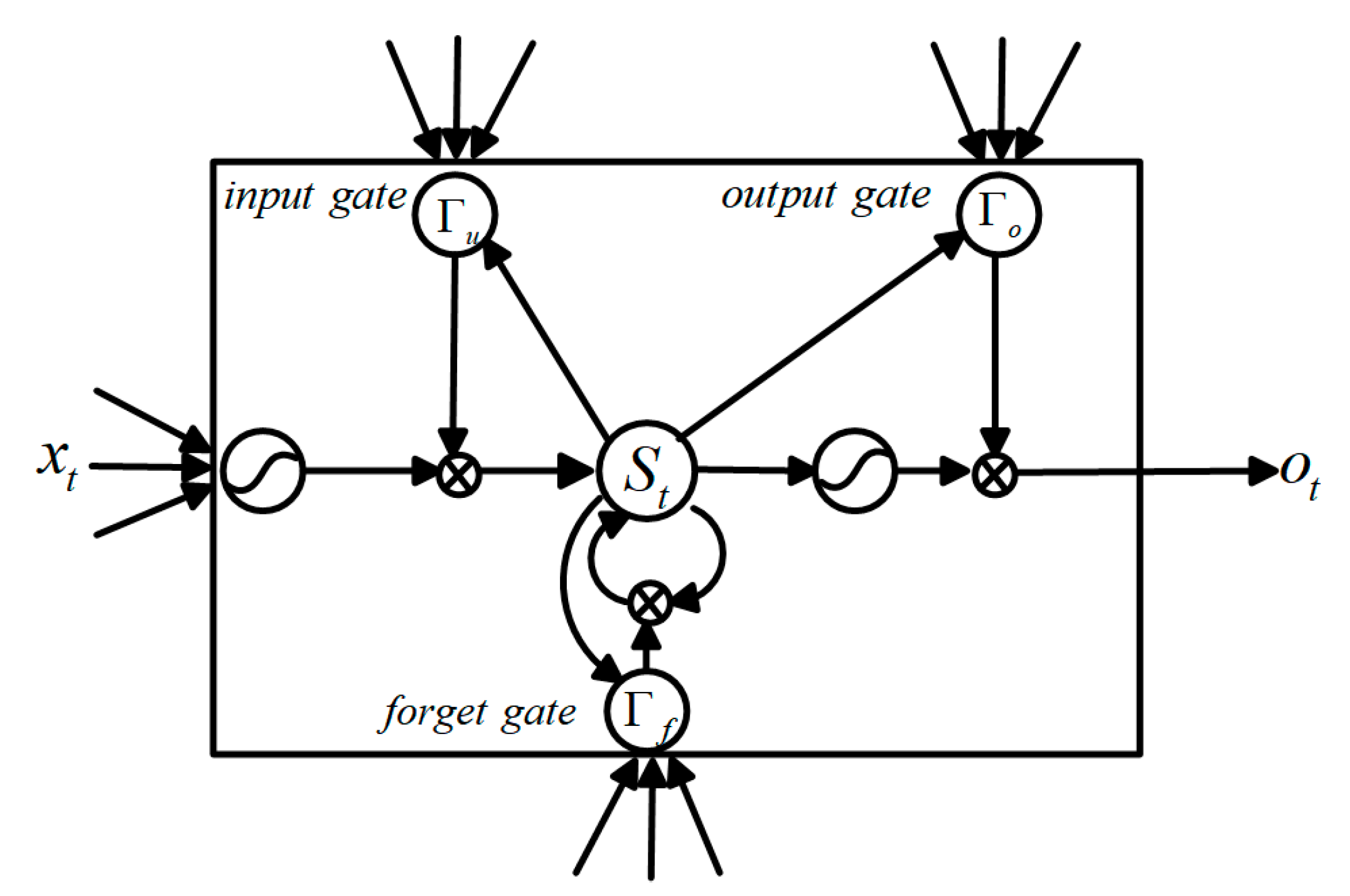
2.2. Long-Short Term Memory
The conventional RNN can only memorize the short time series data. With the increasing amount of data and time steps, it will lose the important information of long term input, causing a vanishing gradient or exploding gradient problem. To tackle this, the LSTM method was proposed in Reference [18], whose structure is shown in Figure 2. LSTM processes the input time series by iteratively passing the transfer function, and adds the input gate (), forget gate () and output gate () for maintaining valuable information of history data. The input gate determines the update of the hidden layer information, whereas the forget gate determines whether the updated information contains the information of the last moment. The output gate determines which part of the information will be selected. Eventually, the formulation of updating the cell states and parameters are as follows:
where is the output at t−1 time slot, and is the input at current moment, is the new candidate values, and is the memory from the current block, is the memory from the previous block, w is the weights, b is the bias, and symbol * is the element-wise multiplier. is another activation function as follows:
2.3. Gated Recurrent Units
Gated Recurrent Units (GRU) is a featured and efficient variant of LSTM. It maintains the effect of LSTM while making the structure simpler, which introduced by Cho et al. [26]. The GRU combines the input gate and the forget gate of LSTM into an update gate , and the output gate in LSTM is named a reset gate () in GRU. $ determines how to combine the new input with the previous memory, and determines how much of the previous memory can pass through. GRU model structure is shown in Figure 3.
The formulation for updating the cell states of GRU and parameters as follows:
The symbols share the same meaning as LSTM except for and . GRU has fewer parameters and thereby benefit from a faster training speed than LSTM.
3. Data Analysis and Forecasting Process
For deep learning method applications, sufficient data to be fed in the model structure is a crucial issue and the key to the successful utilization. In this paper, the big data platform of a company which has a large proportion of EV charging stations in Shenzhen China, one of the largest on-road EV population cities, has been accessed and the data for EV charging loads were obtained and used. This section proposes the preliminaries of data processing methods and the model data formation. Moreover, load forecasting models are addressed.
3.1. Introduction of the Dataset
The dataset provided by a company composes the charging load data of a large charging station from April 2017 to June 2018. Given the complicated practical application, the dataset includes a number of data types, whereas only three featured data types are valuable for the forecasting model. These specific types are charging time, charging quantity and real-time electricity price and have been adopted as input respectively. The Liuyue station has many charging piles. Due to that the vehicle entering the charging station has a strong randomness in time, the selection of the charging pile is also random. The quality of the raw data is low, and it is therefore of importance for data pre-processing to the forecasting model.
3.2. Data Pre-Processing
The data process in this paper is divided into three stages including outlier processing, time interval processing and normalized processing, which are shown as below:
3.2.1. Outlier Processing
The occurrence of an outlier is due to unavoidable interference factors, resulting in errors and missing data in the raw dataset. Corresponding techniques are introduced in this section. For missing data, a load value is first judged in Equation (17), and the mean value of the front and rear data values is used once targeted as a missing outlier according to Equation (18). If the value is larger than the set threshold, the previous data is used instead with the same data type. As for the case where null is present for a certain type of data, the column data is deleted or completed with 0.
when:
where is the load value of the day on time t, is the set threshold, the corresponding outlier data will be replaced by denoted below:
For the error data, a similar operation will be implemented: if the range of the data value exceeds the set threshold, the mean value of the previous and afterwards data values are used instead, being similar to the missing data.
3.2.2. Time Interval Processing
The Python Data Analysis Library e.g., pandas is a NumPy-based tool created for solving data analysis tasks. Pandas incorporates a large number of libraries and standard data models to provide the tools for efficiently processing large scale data sets. In our case, pandas was used to integrate all the charging pile data according to the time point and split them into 24 time points every single day. To get the charging station load data 24 h a day, 10944 rows of data are generated in final.
3.2.3. Normalized Processing
In order to normalize the data, a min-max scaling method is used to scale the data values of input data down to the range of [0,1], which can significantly accelerate the network model training process. The detailed process is shown as follows:
3.3. Load Forecasting Based on Models
In this section, the short-term forecasting framework is given in Figure 4. The framework starts with data pre-processing for the inputs. In this case, the following input features are used:
- The charging load sequence of 24 points per day from April 2017 to June 2018 is denoted as C.
- The charging time sequence of 24 points per day from April 2017 to June 2018 is represented as T.
- The sequence of real-time electricity prices for peak and valley periods is denoted as E. The real-time electricity price has a greater impact on the charging load. Most electric vehicles will choose to charge during the valley price period (23:00–7:00), and the charging load will reach the peak within one day. The charging load is usually at a minimum during the peak price (9:00–12:00, 14:00–17:00, 19:00–21:00).
- The corresponding binary holiday marks H involving the weekday and the weekend are 1 and 2 respectively, and a special holiday is 3.
Due to that, the deep learning models are sensitive to data scale, in this study, we adopt min-max normalization for C, T, E, and the holiday marks H are encoded by one-hot encoder. Eventually, the inputs of the models are 4-dimensional vectors shown as below:
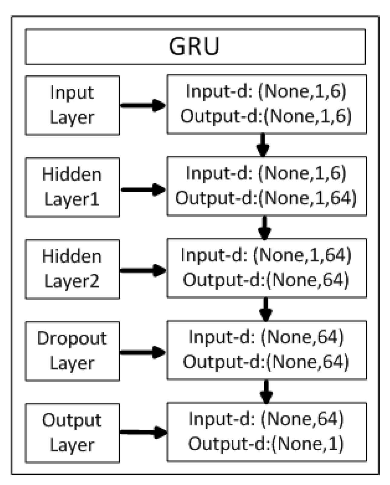
Before establishing the deep learning load forecasting model, we save the data as a file in .csv format and read it in the form of (samples, time steps, features), where the input charge is the charging load at time t−1, and the charging load at time t is taken as the training label, which is shaped like (samples, 1). The model and the label are fed into the network to obtain the pre-training model, the model dimension conversion diagram is shown in Figure 5.
In the training process of the deep learning model, the choice of loss function and optimizer is very important. In this study, we chose mean squared error (MSE) as a loss function, as follows:
where N is the number of samples, is forecasting value, and is actual value.
An effective optimizer is crucial in the deep learning model. In this paper, several optimizers including Adam [27], classic stochastic gradient descent (SGD), Adagrad [28], Adadelta [29] and RMSProp [30], and Adam achieved better results than other optimizers. Therefore, Adam was selected as the optimizer for the training process.
4. Experimental Results and Discussion
In this section, the preprocessed data was fed into four deep learning models for performance evaluation and comparison. All training processes for EV charging load forecasting were implemented in a desktop PC with 3.0 GHz Intel i7 and 64GB of memory, of which the GPU is Geforce Nvidia GTX-1080Ti and all codes are run by Keras library with Tensorflow [31] backend.
4.1. Model Evaluation
To access the effectiveness of the models, two widely used metrics were employed including normalized root mean squared error (NRMSE) and normalized mean absolute error (NMAE) [32]. Given that our data is based on a charging station when all the charging posts of the charging station are not used, the charging load is 0. In this regard, MAPE cannot be used as an evaluation index due to that the denominator is 0. The indicator is normalized because the charging load fluctuates greatly, and it is easier to observe the error size in order to obtain the percentage.
4.2. Experimental Results
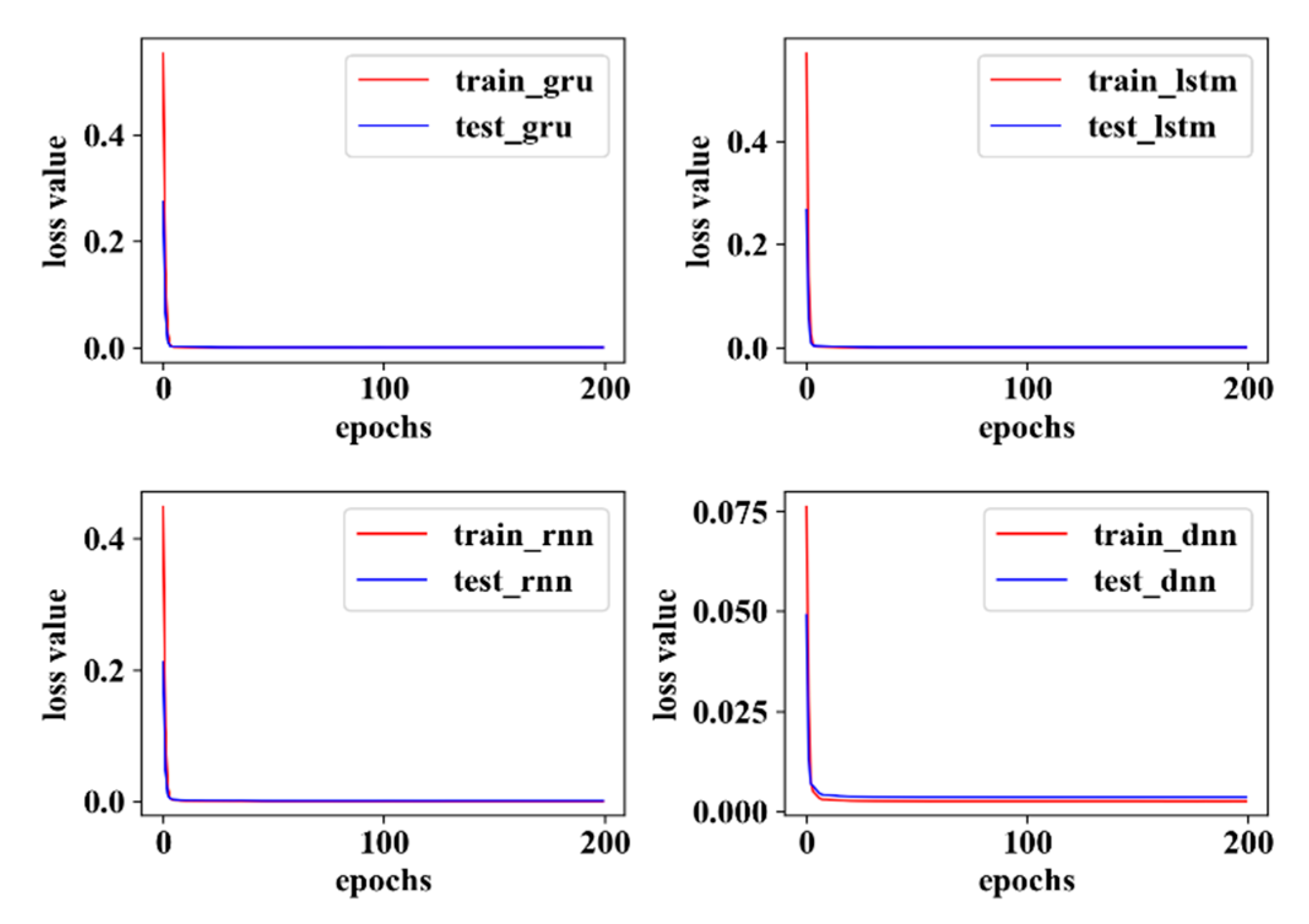
During the training process, the dataset was divided into a training set and a test set, with the ratio selected as 0.7/0.3. As shown in Figure 6, the training set and the test set loss function of the four models can all converge within a limited epoch.
The comparison between the predict values and the actual values of the four models is given by the Figure 7 and Figure 8, Figure 7 demonstrates the results in the testing stage, and Figure 8 illustrates the results in training stage, where the REP denotes real error points. The error denotes the actual value minus the predicted value. Figure 9 and Figure 10 illustrate the results in summer and winter. It can be seen from the figures that the overall charge in summer is high, and there are some no charging periods in the winters. Such difference directly affects the model performance. It can be seen from the figure that the GRU model has the best performance in this case. In Figure 8, the peak load reached at 5 p.m. of the day, and the REP is larger than other points. In Figure 7, the peak load reached at 11 a.m., the REP is also the largest. Although all four models show poor predictive effects on peak loads, the GRU model achieves a comparatively lower REP.
During the experimental process, we modified the number of hidden layers and nodes of the four models, and the performance comparisons are shown in Table 1. It can be seen from the Table 1 that the training process of the deep neural networks (DNN) model was the fastest, costing 68.88 s, whereas the NRMSE and NMAE of the one hidden layer GRU model were minimum, which were as small as 1.48% and 0.47% in training stage respectively, 2.89% and 0.77% in testing stage. However, the multi-hidden layers model had the poorest performance compared to the one hidden layer; it can be seen from the results that although the number of network layers increased, if the other parameters are not changed, not only the training speed is lowered, but also the accuracy is lowered.
5. Conclusions and Future Works
The dramatic increase of EVs exerts significant pressures to the power system operators, and an accurate load forecasting model is a key solution to this problem. In this paper, four deep learning methods were used to predict the short-term charging load of real-world EV charging stations. The results show that the models have demonstrated effectiveness on the dataset, and the one hidden layer GRU model has the best performance compared with the other three models. However, these results cannot prove which model has an absolute advantage in the application. The major reason is that only limited data of one EV charging station was used in the model training, and the number of EVs only accounts for a small part of the actual vehicle numbers. In the future, with the increasing number of EVs and on-line charging behaviors, the amount of data obtained will increase accordingly. Therefore, more influencing factors and an increased amount of data will be considered to increase the dimensions and quality of the features and the quantity of the inputs. New models are promising to improve the prediction speed as well as the forecasting accuracy.
Author Contributions
J.Z. (Juncheng Zhu) and Z.Y. proposes the algorithms and draft the paper. Y.G. and J.Z. (Jiankang Zhang) prepared the data and modified the paper, H.Y. provided the data and setup the experimental environment.
Funding
This research is financially supported by China NSFC under grants 51607177 and 61571401, Natural Science Foundation of Guangdong Province under grants 2018A030310671, China Post-doctoral Science Foundation (2018M631005), Scientific and technological innovation talents in Henan Universities (18HASTIT021).
Conflicts of Interest
The authors declare no conflict of interest.
References
- Raza, M.Q.; Khosravi, A. A review on artificial intelligence based load demand forecasting techniques for smart grid and buildings. Renew. Sustain. Energy Rev. 2015, 50, 1352–1372. [Google Scholar] [CrossRef]
- Lai, C.S.; Jia, Y.; Xu, Z.; Lai, L.L.; Li, X.; Cao, J.; McCulloch, M.D. Levelized cost of electricity for photovoltaic/biogas power plant hybrid system with electrical energy storage degradation costs. Energy Convers. Manag. 2017, 153, 34–47. [Google Scholar] [CrossRef]
- Lai, C.S.; Jia, Y.; Lai, L.L.; Xu, Z.; McCulloch, M.D.; Wong, K.P. A comprehensive review on large-scale photovoltaic system with applications of electrical energy storage. Renew. Sustain. Energy Rev. 2017, 78, 439–451. [Google Scholar] [CrossRef]
- Box, G.E.; Jenkins, G.M.; Reinsel, G.C.; Ljung, G.M. Time Series Analysis: Forecasting and Control; John Wiley & Sons: Hoboken, NJ, USA, 2015. [Google Scholar]
- Li, W.; Zhang, Z.-G. Based on time sequence of ARIMA model in the application of short-term electricity load forecasting. In Proceedings of the 2009 International Conference on Research Challenges in Computer Science, 28–29 December 2009; pp. 11–14. [Google Scholar]
- Haida, T.; Muto, S. Regression based peak load forecasting using a transformation technique. IEEE Trans. Power Syst. 1994, 9, 1788–1794. [Google Scholar] [CrossRef]
- Shankar, R.; Chatterjee, K.; Chatterjee, T.K. A Very Short-Term Load forecasting using Kalman filter for Load Frequency Control with Economic Load Dispatch. J. Eng. Sci. Technol. Rev. 2012, 5, 97–103. [Google Scholar] [CrossRef]
- Park, D.C.; El-Sharkawi, M.A.; Marks, R.J.; Atlas, L.E.; Damborg, M.J. Electric load forecasting using an artificial neural network. IEEE Trans. Power Syst. 1991, 6, 442–449. [Google Scholar] [CrossRef] [Green Version]
- Chen, B.J.; Chang, M.W. Load forecasting using support vector machines: A study on EUNITE competition 2001. IEEE Trans. Power Syst. 2004, 19, 1821–1830. [Google Scholar] [CrossRef]
- Hinton, G.E.; Osindero, S.; Teh, Y.W. A fast learning algorithm for deep belief nets. Neural Comput. 2006, 18, 1527–1554. [Google Scholar] [CrossRef]
- Hippert, H.S.; Pedreira, C.E.; Souza, R.C. Neural networks for short-term load forecasting: A review and evaluation. IEEE Trans. Power Syst. 2001, 16, 44–55. [Google Scholar] [CrossRef]
- Long, J.; Shelhamer, E.; Darrell, T. Fully convolutional networks for semantic segmentation. In Proceedings of the IEEE Conference on Computer Vision and Pattern Recognition, Boston, MA, USA, 7–12 June 2015; pp. 3431–3440. [Google Scholar]
- Krizhevsky, A.; Sutskever, I.; Hinton, G.E. Imagenet classification with deep convolutional neural networks. In Proceedings of the Advances in Neural Information Processing Systems, Lake Tahoe, NV, USA, 3–6 December 2012; pp. 1097–1105. [Google Scholar]
- Girshick, R.; Donahue, J.; Darrell, T.; Malik, J. Rich feature hierarchies for accurate object detection and semantic segmentation. In Proceedings of the IEEE Conference on Computer Vision and Pattern Recognition, Washington, DC, USA, 24–27 June 2014; pp. 580–587. [Google Scholar]
- Sutskever, I.; Vinyals, O.; Le, Q.V. Sequence to sequence learning with neural network. In Proceedings of the Advances in Neural Information Processing Systems, Montreal, QC, Canada, 8–13 December 2014; pp. 3104–3112. [Google Scholar]
- Vermaak, J.; Botha, E.C. Recurrent neural networks for short-term load forecasting. IEEE Trans. Power Syst. 1998, 13, 126–132. [Google Scholar] [CrossRef]
- Marino, D.L.; Amarasinghe, K.; Manic, M. Building energy load forecasting using deep neural networks. In Proceedings of the IECON 2016—42nd Annual Conference of the IEEE Industrial Electronics Society, Florence, Italy, 24–27 October 2016; pp. 7046–7051. [Google Scholar]
- Hochreiter, S.; Schmidhuber, J. Long short-term memory. Neural Comput. 1997, 9, 1735–1780. [Google Scholar] [CrossRef]
- Kong, W.; Dong, Z.Y.; Jia, Y.; Hill, D.J.; Xu, Y.; Zhang, Y. Short-term residential load forecasting based on LSTM recurrent neural network. IEEE Trans. Smart Grid 2017, 10, 841–851. [Google Scholar] [CrossRef]
- Bouktif, S.; Fiaz, A.; Ouni, A.; Serhani, M. Optimal deep learning lstm model for electric load forecasting using feature selection and genetic algorithm: Comparison with machine learning approaches. Energies 2018, 11, 1636. [Google Scholar] [CrossRef]
- Zheng, H.; Yuan, J.; Chen, L. Short-term load forecasting using EMD-LSTM neural networks with a Xgboost algorithm for feature importance evaluation. Energies 2017, 10, 1168. [Google Scholar] [CrossRef]
- Gensler, A.; Henze, J.; Sick, B.; Raabe, N. Deep Learning for solar power forecasting—An approach using AutoEncoder and LSTM Neural Networks. In Proceedings of the 2016 IEEE International Conference on Systems, Man, and Cybernetics (SMC), Budapest, Hungary, 9–12 October 2016; pp. 002858–002865. [Google Scholar]
- Kumar, J.; Goomer, R.; Singh, A.K. Long short term memory recurrent neural network (lstm-rnn) based workload forecasting model for cloud datacenters. Procedia Comput. Sci. 2018, 125, 676–682. [Google Scholar] [CrossRef]
- Kuan, L.; Yan, Z.; Xin, W.; Yan, C.; Xiangkun, P.; Wenxue, S.; Zhe, J.; Yong, Z.; Nan, X.; Xin, Z. Short-term electricity load forecasting method based on multilayered self-normalizing GRU network. In Proceedings of the 2017 IEEE Conference on Energy Internet and Energy System Integration (EI2), Beijing, China, 26–28 November 2017; pp. 1–5. [Google Scholar]
- Yunyan, L.; Yuansheng, H.; Meimei, Z. Short-Term Load Forecasting for Electric Vehicle Charging Station Based on Niche Immunity Lion Algorithm and Convolutional Neural Network. Energies 2018, 11, 1253. [Google Scholar] [Green Version]
- Cho, K.; Van Merriënboer, B.; Bahdanau, D.; Bengio, Y. On the properties of neural machine translation: Encoder-decoder approaches. arXiv 2014, arXiv:1409.1259. [Google Scholar]
- Kingma, D.P.; Ba, J. Adam: A method for stochastic optimization. arXiv 2014, arXiv:1412.6980. [Google Scholar]
- Duchi, J.; Hazan, E.; Singer, Y. Adaptive subgradient methods for online learning and stochastic optimization. J. Mach. Learn. Res. 2011, 12, 2121–2159. [Google Scholar]
- Zeiler, M.D. ADADELTA: An adaptive learning rate method. arXiv 2012, arXiv:1212.5701. [Google Scholar]
- Tieleman, T.; Hinton, G. Lecture 6.5-rmsprop: Divide the gradient by a running average of its recent magnitude. COURSERA Neural Netw. Mach. Learn. 2012, 4, 26–31. [Google Scholar]
- Abadi, M.; Barham, P.; Chen, J.; Chen, Z.; Davis, A.; Dean, J.; Devin, M.; Ghemawat, S.; Irving, G.; Isard, M.; Kudlur, M. Tensorflow: A system for large-scale machine learning. In Proceedings of the 12th USENIX Symposium on Operating Systems Design and Implementation (OSDI’16), Savannah, GA, USA, 2–4 November 2016; pp. 265–283. [Google Scholar]
- Willmott, C.J.; Ackleson, S.G.; Davis, R.E.; Feddema, J.J.; Klink, K.M.; Legates, D.R.; O’donnell, J.; Rowe, C.M. Statistics for the evaluation and comparison of models. J. Geophys. Res. Oceans 1985, 90, 8995–9005. [Google Scholar] [CrossRef]
Figure 1.
Basic recurrent neural networks structure.

Figure 2.
Basic long short-term memory structure.

Figure 3.
Basic gated recurrent units structure.

Figure 4.
Deep learning model based forecasting framework.

Figure 5.
Model dimension conversion diagram.

Figure 6.
Loss curve of the four models.

Figure 7.
Predictions and real error points (REP) of the test stage.

Figure 8.
Predictions and REP of the training stage.

Figure 9.
Predictions and REP of the summer scenario.

Figure 10.
Predictions and REP of the winter scenario.


Table 1.
Performance comparison of deep learning based methods. NRMSE: normalized root mean squared error, NMAE: normalized mean absolute error, DNN: deep neural networks, RNN: recurrent neural networks, LSTM: long short term memory; GRU: gated recurrent units.
Table 1.
Performance comparison of deep learning based methods. NRMSE: normalized root mean squared error, NMAE: normalized mean absolute error, DNN: deep neural networks, RNN: recurrent neural networks, LSTM: long short term memory; GRU: gated recurrent units.
| Model | Hidden Layers | Train-NRMSE (%) | Test-NRMSE (%) | Train-NMAE (%) | Test-NMAE (%) |
|---|---|---|---|---|---|
| DNN | 2 3 4 | 2.05 1.97 1.98 | 3.69 3.79 3.81 | 1.06 0.50 0.46 | 1.32 0.94 0.92 |
| RNN | 1 2 3 | 1.50 1.52 1.61 | 2.91 2.91 2.96 | 0.62 0.70 0.84 | 0.91 1.01 1.19 |
| LSTM | 1 2 3 | 1.71 1.71 1.74 | 3.36 3.36 3.39 | 0.59 0.79 0.68 | 0.90 1.11 1.01 |
| GRU | 1 2 3 | 1.48 1.56 1.52 | 2.89 2.92 2.91 | 0.47 0.48 0.51 | 0.77 0.78 0.84 |
© 2019 by the authors. Licensee MDPI, Basel, Switzerland. This article is an open access article distributed under the terms and conditions of the Creative Commons Attribution (CC BY) license (http://creativecommons.org/licenses/by/4.0/).
Share and Cite
MDPI and ACS Style
Zhu, J.; Yang, Z.; Guo, Y.; Zhang, J.; Yang, H. Short-Term Load Forecasting for Electric Vehicle Charging Stations Based on Deep Learning Approaches. Appl. Sci. 2019, 9, 1723. https://doi.org/10.3390/app9091723
AMA Style
Zhu J, Yang Z, Guo Y, Zhang J, Yang H. Short-Term Load Forecasting for Electric Vehicle Charging Stations Based on Deep Learning Approaches. Applied Sciences. 2019; 9(9):1723. https://doi.org/10.3390/app9091723
Chicago/Turabian StyleZhu, Juncheng, Zhile Yang, Yuanjun Guo, Jiankang Zhang, and Huikun Yang. 2019. "Short-Term Load Forecasting for Electric Vehicle Charging Stations Based on Deep Learning Approaches" Applied Sciences 9, no. 9: 1723. https://doi.org/10.3390/app9091723
Note that from the first issue of 2016, this journal uses article numbers instead of page numbers. See further details here.