A Model to Predict Acoustic Resonant Frequencies of Distributed Helmholtz Resonators on Gas Turbine Engines

Featured Application

Passive control devices for combustion instability and combustion noise in gas turbine engines.

Abstract

Helmholtz resonators, traditionally designed as a narrow neck backed by a cavity, are widely applied to attenuate combustion instabilities in gas turbine engines. The use of multiple small holes with an equivalent open area to that of a single neck has been found to be able to significantly improve the noise damping bandwidth. This type of resonator is often referred to as “distributed Helmholtz resonator”. When multiple holes are employed, interactions between acoustic radiations from neighboring holes changes the resonance frequency of the resonator. In this work, the resonance frequencies from a series of distributed Helmholtz resonators were obtained via a series of highly resolved computational fluid dynamics simulations. A regression analysis of the resulting response surface was undertaken and validated by comparison with experimental results for a series of eighteen absorbers with geometries typically employed in gas turbine combustors. The resulting model demonstrates that the acoustic end correction length for perforations is closely related to the effective porosity of the perforated plate and will be obviously enhanced by acoustic radiation effect from the perforation area as a whole. This model is easily applicable for engineers in the design of practical distributed Helmholtz resonators.

1. Introduction

Helmholtz resonators are commonly employed to reduce sound pressure levels across a broad range of applications, including the built environment, industrial installations, and propulsion devices, such as gas turbines [1,2,3]. Combustion instability represents a significant problem in the application of low NOx emission LPC (lean premixed combustion) gas turbines. Helmholtz resonators are commonly applied to achieve attenuation effect near the instability frequencies. However, attenuation bandwidth due to Helmholtz resonance effect is often very narrow. In comparison, attenuation of noise by distributed Helmholtz resonators takes place within a much wider frequency range thanks to the stronger acoustic resistance of those smaller perforations [1,2,3].

The distributed Helmholtz resonator can be thought of as a special type of perforated plate absorber (PPA). The noise attenuation effect of a PPA is typically characterized by its peak damping frequency and absorption bandwidth. The peak damping frequency often coincides with the resonance frequency of a PPA [4,5,6,7]:

$$f_r=\frac{c}{2\pi }\sqrt{\frac{A}{V{l}_e}}$$

(1)

$$l_e=l+l_{ec}=l+0.96\sqrt{A_0}$$

(2)

where $f_r$ stands for resonance frequency, c represents the speed of sound, $V$ represents the volume of the resonator cavity, $A$ is the total opening area of all perforates, $l_e$ is effective length of the opening, which includes the physical plate thickness $l$ and an acoustic radiation “end effect” length $l_{ec}$. $A_0$ is the cross section area of an individual perforation.

A distributed Helmholtz resonator with multiple small holes is able to significantly improve the noise damping bandwidth compared to a single neck Helmholtz absorber. On the other hand, when multiple holes are employed, additional acoustic interaction occurs between neighboring holes, thereby changing the resonance frequency of the resonator.

A number of researchers, including Ingard [5], Fok [8], and Atalla [9], have demonstrated that the end correction length is affected by the interaction effect between neighboring perforations. Fok [8] tested an orifice in the center of a partition across a tube and proposed that to take into account the effect of hole interaction, the end correction length for the orifice should be corrected by a “Fok’s function”, $\psi$ [8]:

$$\psi ={(1-1.4092\xi +0.33818{\xi }^3+0.06793{\xi }^5-0.02287{\xi }^6+0.03015{\xi }^7-0.01641{\xi }^8)}^{-1}$$

(3)

where $\xi$ is the hole diameter (d) divided by hole separation distance (b).

Fok’s function is later cited by other authors to consider the effect of hole interaction on acoustic radiation strength [10,11,12,13,14]. The acoustic effective length of the perforated plate then becomes:

$$l_e=l+l_{ec}=l+\frac{0.96\sqrt{A_0}}{\psi \left(\xi \right)}$$

(4)

Substituting for Fok’s function gives,

$$l_e=l+0.96\sqrt{A_0} \left(1-1.4092\xi +0.33818{\xi }^3+0.06793{\xi }^5-0.02287{\xi }^6+0.03015{\xi }^7-0.01641{\xi }^8\right)$$

As shown in Figure 1, where Fok’s function is plotted against hole diameter (d) divided by hole separation distance (b), Fok’s function is always greater than 1 and increases with increasing d/b. Fok’s function appears in the denominator in Equation (4), therefore, the acoustic end correction length $0.96\sqrt{A_0}$ gradually diminishes with decreasing hole separation distance due to hole interaction effect. Melling [10] provided an explanation for the diminishing end correction by a simple diagram, as illustrated in Figure 2. He described the end correction effect as being the result of an “attached air mass” in the neighborhood of the perforation. Melling [10] claimed that a portion of “attached masses” for a perforation will overlap with the neighboring perforations if they are sufficiently close to each other. The overlapped portions of attached masses merge into one portion of attached mass, and as a result the average attached mass for each perforation is reduced. However, Melling [10] did not provide an explanation about the underlying physics of why the two merged “attached masses” would merge and result in a reduced total “attached mass”.

Ingard [5] developed a mathematical model to describe the acoustic effect upon a single hole from the neighboring holes. He found that hole–hole interaction effect will increase the end correction magnitude. Rachevkin [12] stated that when small holes are in extreme proximity to each other, they will act as a big hole in terms of their impact on passing acoustic field. Therefore, in this situation, the overall acoustic radiation effect is not only generated by each single hole, but also the perforation region as a whole. Tayong [14,15] proposed a “geometrical tortuosity model” to account for the acoustic radiation effect of the perforation region as a whole, which he called “heterogeneity distribution effects”. However, the exact definition of parameters such as tortuosity in these models require external input and remains difficult for engineers when it comes to designing industrial distributed resonators.

In this paper, the acoustic end correction effect for distributed Helmholtz resonators or PPA’s, in which holes are in proximity with each other, is conveniently proposed to be a combination of two radiation effects—the acoustic radiation effect by each single orifice and the acoustic radiation effect by the overall perforation area. This paper will also propose an easily applicable model for the prediction of resonance frequencies of resonators. This resulting model will be of significant value in the design of practical distributed Helmholtz absorbers, especially those distributed Helmholtz resonators applied on gas turbine engines to control combustion instabilities.

2. Materials and Methods

2.1. Numerical Simulation

In order to investigate acoustic propagation through small holes, a time-accurate, three dimensional, numerical solution was obtained for the propagation of a white noise signal in an impedance tube, in the absence of any mean flow or bias flow, under the assumption that the acoustic perturbations may be considered to remain in the laminar flow regime. The propagation of an acoustic plane wave in an impedance tube, an incident normal to a perforated plate, as show in Figure 3, may be represented as an unsteady compressible laminar flow. Simulation of such flow regimes does not require significant modeling approximations, and therefore, in the context of this application, may be considered to be a direct numerical solution to the governing Navier-Stokes equations, provided satisfactory temporal and spatial resolution have been demonstrated.

Computational Fluid Dynamics (CFD) is based upon the numerical solution of the underlying governing equations for fluid flow under specified boundary conditions. The method has been successfully applied by a number of authors to study acoustic radiation effect for multi-perforated plate absorbers [16,17,18,19]. The simulated acoustic source applied in this work was a white noise signal ranging between 100 Hz and 1000 Hz with a 100 dB overall sound pressure level. The governing equations may be expressed, for brevity alone, in axisymmetric cylindrical polar coordinates as:

$$\frac{\partial \rho }{\partial t}+\frac{\partial \left(\rho u_x\right)}{\partial x}+\frac{1}{r}\frac{\partial \left(\rho r{u}_r\right)}{\partial r}=0$$

(5)

$$\frac{\partial \left(\rho u_x\right)}{\partial t}+\frac{1}{r}\frac{\partial \left(\rho r{u}_x{u}_x\right)}{\partial x}+\frac{1}{r}\frac{\partial \left(\rho r{u}_r{u}_x\right)}{\partial r}=\frac{\partial {\tau }_{rx}}{\partial r}-\frac{\partial p}{\partial x}+S_x$$

(6)

$$\frac{\partial \left(\rho u_r\right)}{\partial t}+\frac{1}{r}\frac{\partial \left(\rho r{u}_x{u}_r\right)}{\partial x}+\frac{1}{r}\frac{\partial \left(\rho r{u}_r{u}_r\right)}{\partial r}=\frac{\partial {\tau }_{xr}}{\partial x}-\frac{\partial p}{\partial r}+S_r$$

(7)

$$\frac{\partial \left(\rho h\right)}{\partial t}+\frac{1}{r}\frac{\partial \left(\rho r{u}_{x}h\right)}{\partial x}+\frac{1}{r}\frac{\partial \left(\rho r{u}_{r}h\right)}{\partial r}=\frac{1}{r}\frac{\partial }{\partial x}\left(r\Gamma \frac{\partial h}{\partial x}\right)+\frac{1}{r}\frac{\partial }{\partial r}\left(r\Gamma \frac{\partial h}{\partial r}\right)+S_h$$

(8)

where $x,r$ are the axial and radial directions of the cylindrical coordinate system and $u_x,u_r$ are the axial and radial velocities, $t$ represents time, ${\tau }_{rx}$ is the axial direction viscous stress due to flow velocity gradient in radial directions. $S_x,S_r$ are momentum source terms; $h$ is the enthalpy and $S_h$ the source term of the energy equation. The ideal gas equation of state, $p=\rho RT$, is employed to determine the density of the compressible fluid, where $p,\rho ,T,R$ represent the absolute pressure, density, temperature of the medium, and the gas constant, respectively.

The discretized spatial terms were approximated by a second order biased upwind scheme, which provides both the numerical accuracy of the second order upwind scheme and the convergence robustness of the first order scheme [20]. The discretized temporal terms were approximated by a bounded second order accurate, implicit scheme, to robustly resolve the rapidly fluctuating pressure signal [20]. All simulations were undertaken with the double precision version of ANSYS FLUENT 17.2. A general non-reflecting boundary condition proposed by Poinsot et. al. [21,22] is applied to represent anechoic boundaries in CFD simulations.

A two-microphone transfer function was employed for acoustic analysis [23]. The normalized specific acoustic impedance of the plate absorber is defined by Kuttruff [4] as:

$$z=r+ix=\left(1+R\right)/\left(1-R\right)$$

(9)

where $r$ is the normalized specific acoustic resistance, which is a measure of the resistance that the perforated plate presents to the acoustic flow, $x$ is the normalized specific acoustic reactance, which describes the phase difference between the driving pressure difference and the resultant orifice velocity. $R$ represents the reflection coefficient. For a PPA installed at the end of an impedance tube, the acoustic energy that is not reflected by the absorber is absorbed by the PPA and the acoustic energy absorption coefficient, therefore, becomes [4]:

$$\alpha =1-{\left|R\right|}^2=\frac{4r}{{(1+r)}^2+x^2}$$

(10)

As can be seen from Equation (10), the optimum absorption effect of a PPA takes place at the frequency where acoustic reactance is zero, which also coincides with the resonance frequency of a PPA [4].

The range of geometric configurations considered is summarized in

Table 1. Geometric features of the plates resolved by CFD.

Case No.	Diameter of the Impedance Tubes and Perforated Plates (mm)	Diameter of the Hole, d (mm)	x/d	y/d	$\mathbf{Effective} \mathbf{Porosity}, {\mathit{\sigma }}_{\mathit{e}\mathit{f}\mathit{f}}$
1	90	2	1.2	1.2	0.545
2	90	2	1.5	1.5	0.349
3	90	2	2	2	0.196
4	90	2	2.5	2.5	0.126
5	90	2	3	3	0.087
6	90	2	4	4	0.049
7	90	2	5	5	0.031
8	135	3	1.2	1.2	0.545
9	135	3	1.5	1.5	0.444
10	135	3	2	2	0.250
11	135	3	2.5	2.5	0.160
12	135	3	3	3	0.111
13	135	3	4	4	0.063
14	135	3	5	5	0.040
15	180	4	1.2	1.2	0.545
16	180	4	1.5	1.5	0.444
17	180	4	2	2	0.250
18	180	4	2.5	2.5	0.160
19	180	4	3	3	0.111
20	180	4	4	4	0.063
21	180	4	5	5	0.040
22	135	3	1.5	5	0.105
23	135	3	2	5	0.079
24	135	3	3	5	0.052
25	135	3	4	5	0.039

CFD: Abbreviation for “Computational Fluid Dynamics”; x: hole separation distance in the horizontal direction as shown in Figure 4; y: hole separation distance in the vertical direction as shown in Figure 4; ${\sigma }_{eff}$: effective porosity as defined in Equation (11).

. All plates have the same porosity of 0.0123 and the same thickness of 2.5 mm. Figure 4 illustrates a selection of the geometric configurations considered. The ratios of hole separation distance to hole diameter (x/d, y/d) vary from 1.2, to 1.5, 2, 2.5, 3, 4, 5, where x is the hole pitch in the horizontal direction, y is the hole pitch in the vertical direction, and d is the diameter of the hole.

The size of the perforations varies from 2 mm to 3 mm and 4 mm. Those plates with 2 mm, 3 mm, and 4 mm perforations are installed in impedance tubes with diameters of 90 mm, 135 mm, and 180 mm, respectively. The length of all orifices is kept consistent at 2.5 mm. All plates are backed by a 25 mm deep cylindrical air cavity, which has an identical cross-section to upstream impedance tubes. Real world perforated plates are sometimes more densely perforated in one direction than in other directions; therefore, perforated plates (plate 23, plate 24, and plate 25) with different aspect ratios were taken into consideration as well.

The porosity of a perforated plate is defined as the ratio of the total opening area to the whole surface area of the perforated plate, $\sigma =n{A}_0/A_p=A/A_p$, where $n$ is the number of holes, which equals to 25 for the PPA simulated in this work and 32 for those experimentally tested.

In the above definition, $A_0$ is the cross-section area of a single hole, $A$ represents the total opening area of all holes, and $A_p$ stands for the total surface area of the perforated plate backed by a cavity. In this paper, a new parameter, effective porosity, is introduced, and for a parallel distributed plate, as shown in Figure 4, it is defined to be:

$${\sigma }_{eff}=\pi d^2/4xy$$

(11)

where $d$ is diameter of the hole, $x$ and $y$ are hole separation distance in two directions, as shown in Figure 4, $\pi d^2/4$ is the opening area in a rectangular perforation region whose area is $xy$. Effective porosity depicts the uniformity of hole distribution in a perforated plate backed by a cavity. It is equal to classical porosity if all holes are distributed evenly on a perforated surface. It will be larger than the classical porosity if some or all holes are more densely distributed in a local area of a noise damping surface.

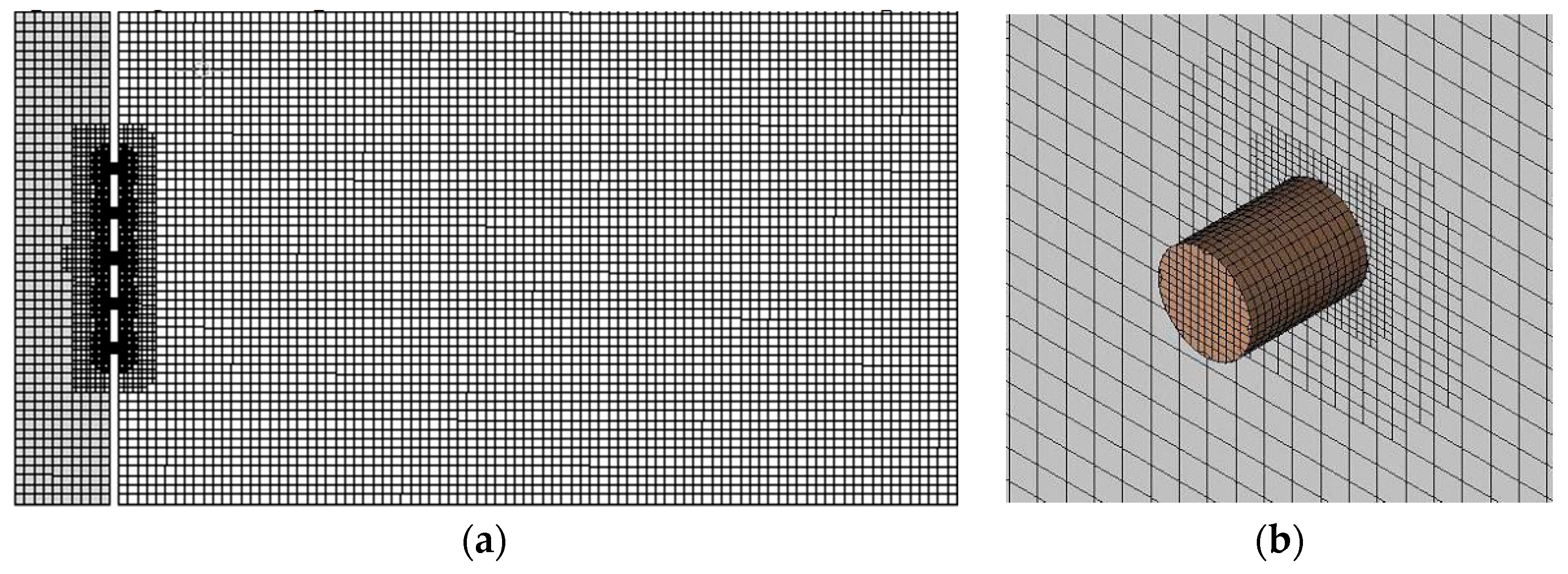
The phenomena of acoustic radiation takes place in close proximity to the individual holes in the perforated plate. Therefore, this requires a computational grid of sufficient resolution to capture the local fluid dynamic and acoustic phenomena. The structural composition of the computational grid employed in this work is illustrated in Figure 5. Block-structured meshes with a cell size of 2.6 mm were built within the air cavity and impedance tubes, as shown in Figure 5a, and block-structured meshes were further refined near the orifices until the mesh size reached a minimum of 0.2 mm in the orifice, as shown in Figure 5b. A further mesh with a resolution of 0.1 mm in the orifice was generated for a separate test of grid dependency.

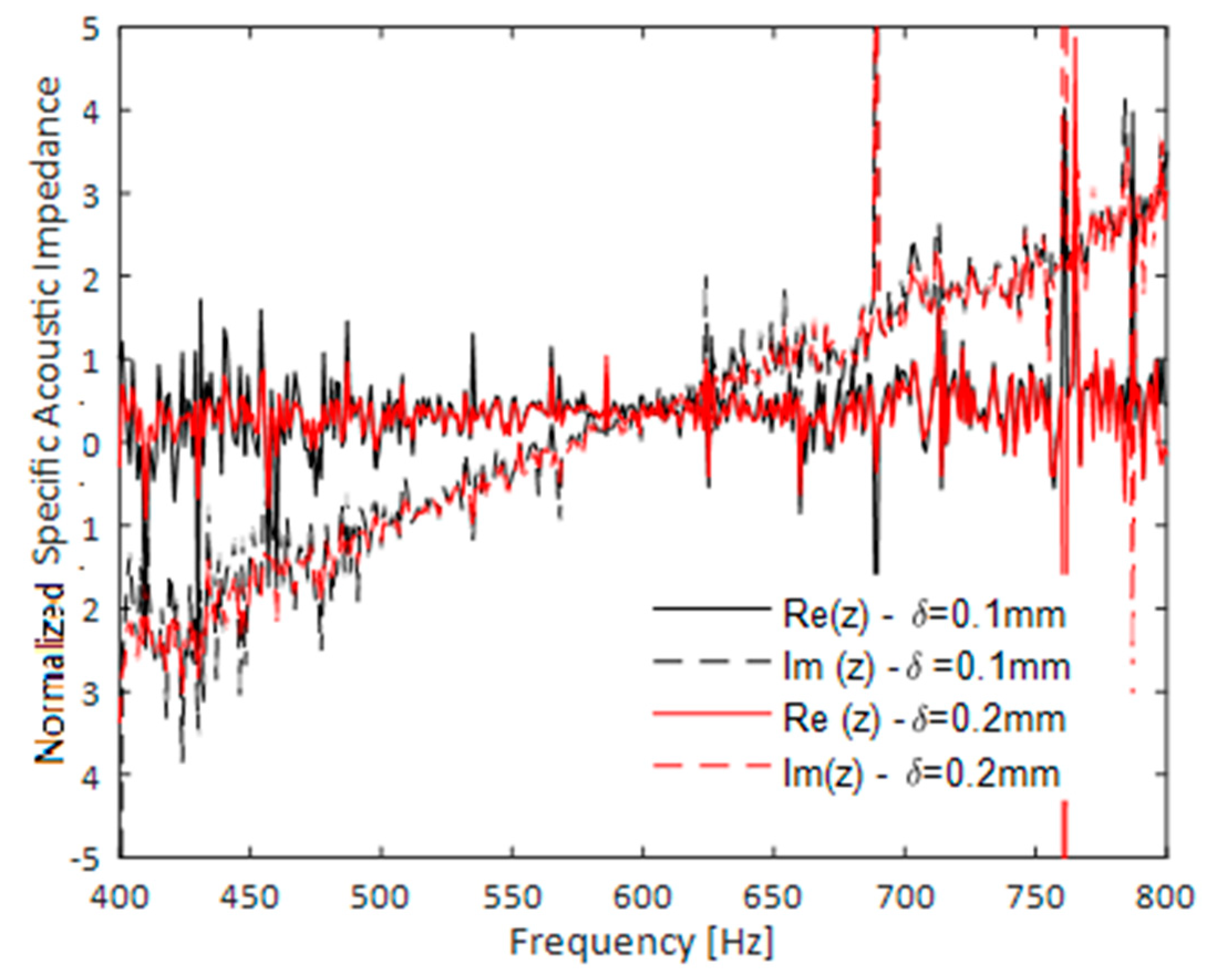
Figure 6 illustrates the normalized specific acoustic impedance determined from the simulation for perforated plate No.7, employing both the 0.2 mm and the 0.1 mm resolution computational grids. The results show a very similar character and support the use of the 0.2 mm resolution grid as being an acceptable grid-independent solution for acoustic impedance.

2.2. Experimental Validation

Simulation of the acoustic signal propagation through a distributed Helmholtz resonator was undertaken by using a laminar flow solver, which itself is free from significant physical models. Verification of the solution methodology in the form of numerical errors associated with the quadrature scheme and discretization can be achieved by the selection of high order numerical schemes and demonstrated through a test of grid dependency.

In order to provide a validation of the results from the computational simulations, experimental data was collected for eighteen separate plates in a dedicated experimental test rig, illustrated in Figure 7 and Figure 8.

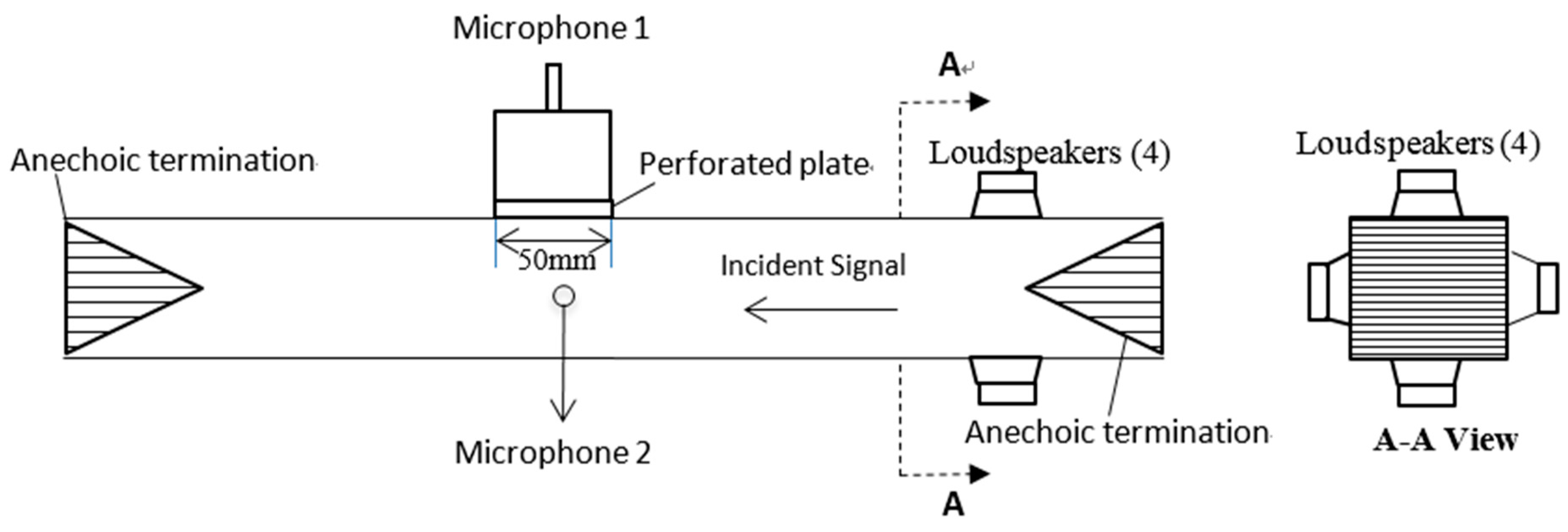
The test rig (Figure 7) consists of an upstream duct section, a downstream duct section, and a test section installed in between them, each with an internal diameter of 165 mm. Four opposing loudspeakers were installed on the upstream duct. The test rig was designed to include anechoic terminations to minimize reflections from the change in impedance at the inlet and exit. In all test configurations, no mean flow through the duct or bias flow through the plates was applied.

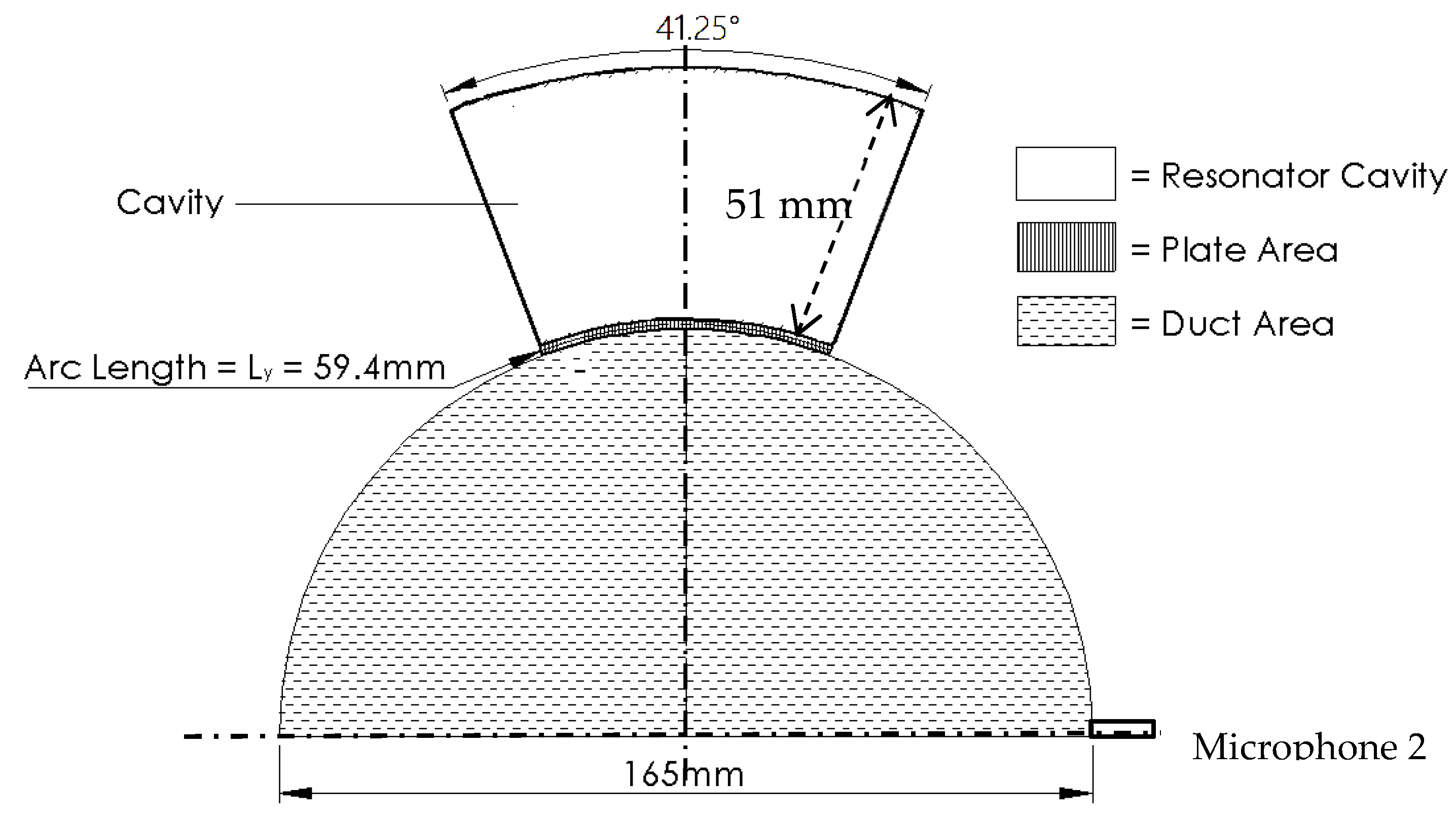
The resonant cavity, Figure 8, was constructed from a curved rectangular test plate with a length of 0.05 m and an arc length of 0.0594 m, mounted flush to the side wall of the test section duct, with an attached fan-shaped cavity of 0.051 m depth. Referring to Figure 8, the volume of the cavity is:

$$V=\pi [{(0.051+0.165/2+\mathrm{}0.002)}^2-\left(0.165/2+\mathrm{}0.002{)}^2\right]\times \frac{{41.25}^{°}}{{360}^{°}}\times 0.05=\mathrm{}0.002 {\mathrm{m}}^3$$

(12)

where 51 mm is the cavity depth, 165 mm is the internal diameter of the tube, 2 mm is the thickness of plate, and 41.25° represents the angle of the fan-shaped cavity.

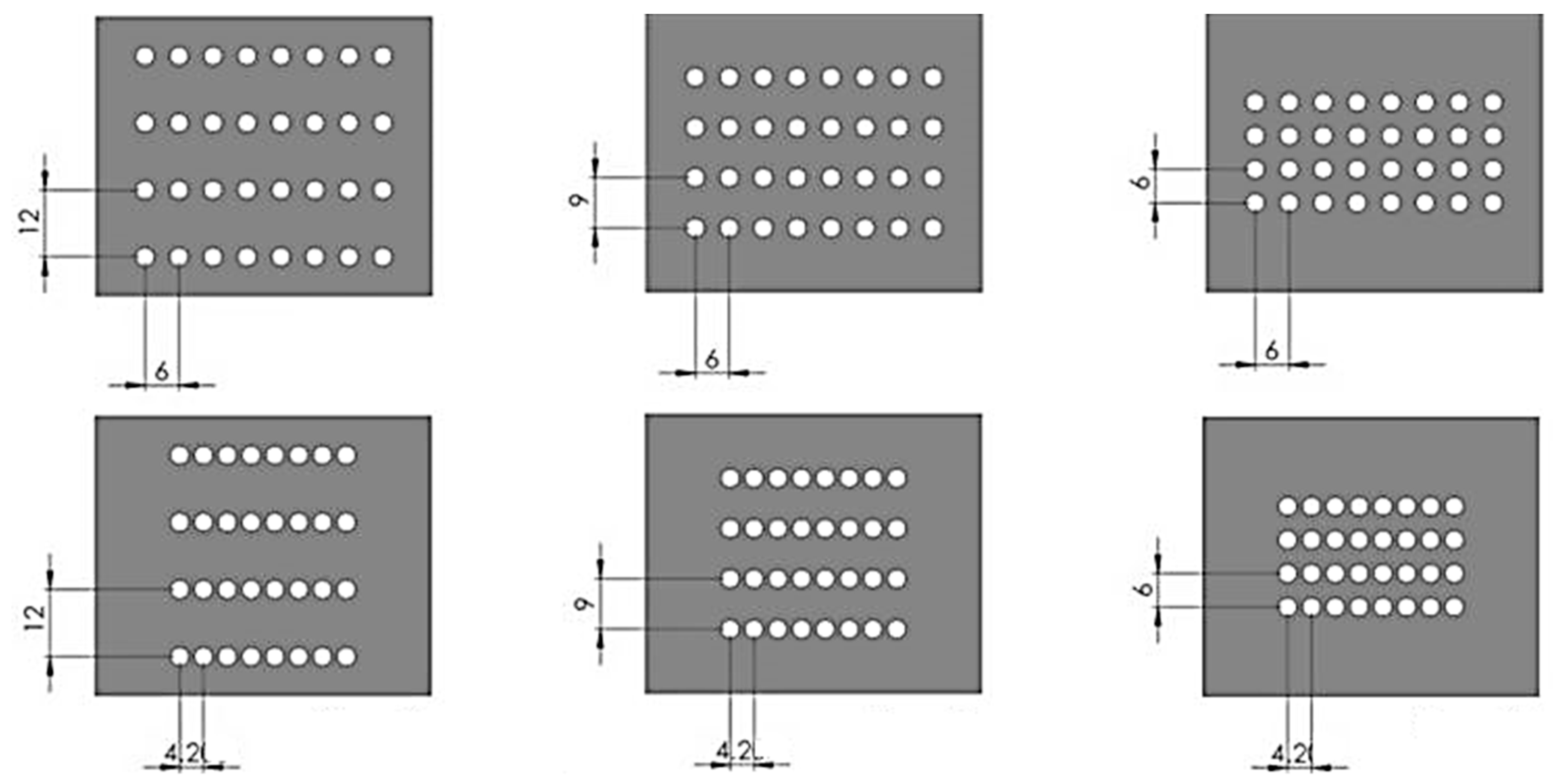
A total of 32 circular perforations, as exemplified in Figure 9, were drilled in the x and y directions, respectively. The diameters of these orifices were 2 mm, 3 mm, or 4 mm. The thickness of all experimentally tested plates was kept the same at 2 mm.

Detailed geometric features of the orifices are exemplified in Figure 9 and detailed in

Table 2. Geometric details of perforated plates for experimental data collection.

Case # EXP	Diameter (mm)	Plate Circumferential Length (mm)	Plate Axial Length (mm)	Hole Distance-x (mm)	Hole Distance-y (mm)	$\mathbf{Porosity} \mathit{\sigma }$	$\mathbf{Effective} \mathbf{Porosity} {\mathit{\sigma }}_{\mathit{e}\mathit{f}\mathit{f}}$
1	2.0	59.4	50	6.0	12	0.0338	0.0436
2	2.0	59.4	50	6.0	9	0.0338	0.0582
3	2.0	59.4	50	6.0	6	0.0338	0.0873
4	2.0	59.4	50	4.2	12	0.0338	0.0623
5	2.0	59.4	50	4.2	9	0.0338	0.0831
6	2.0	59.4	50	4.2	6	0.0338	0.1247
7	3.0	59.4	50	6.0	12	0.0762	0.0982
8	3.0	59.4	50	6.0	9	0.0762	0.1309
9	3.0	59.4	50	6.0	6	0.0762	0.1963
10	3.0	59.4	50	4.2	12	0.0762	0.1402
11	3.0	59.4	50	4.2	9	0.0762	0.1870
12	3.0	59.4	50	4.2	6	0.0762	0.2805
13	4.0	59.4	50	6.0	12	0.135	0.1745
14	4.0	59.4	50	6.0	9	0.135	0.2327
15	4.0	59.4	50	6.0	6	0.135	0.3491
16	4.0	59.4	50	4.2	12	0.135	0.2493
17	4.0	59.4	50	4.2	9	0.135	0.3324
18	4.0	59.4	50	4.2	6	0.135	0.4987

EXP: Abbreviation for “Experiment”; x: hole separation distance in the horizontal direction as shown in Figure 9; y: hole separation distance in the vertical direction as shown in Figure 9; ${\sigma }_{eff}$: effective porosity as defined in Equation (11).

. A signal generator and amplification was employed to generate a 100 dB white noise signal within a bandwidth of 100 Hz–1000 Hz. Two microphones were installed flush with the resonator top wall and the acoustic duct wall, respectively. The resulting magnitude of the pressure response function, PRF, is defined below, based upon the Fast Fourier Transform (FFT) of the individual microphone signals:

$$PRF=\left|\frac{FFT\left(P\_acoustic\_microphone\_1\right)}{FFT\left(P\_acoustic\_microphone\_2\right)}\right|$$

3. Results

3.1. Acquisition of Model

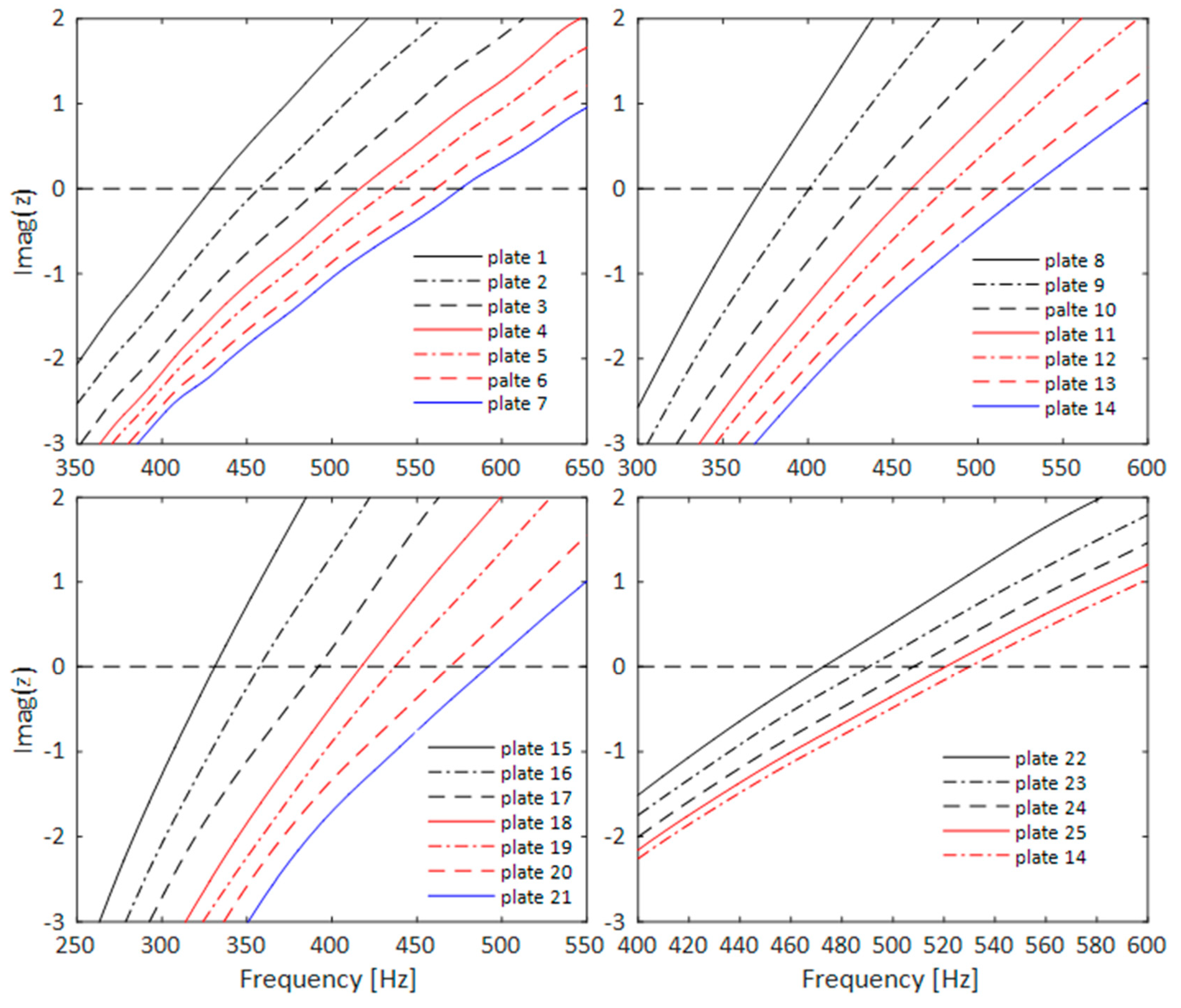
Figure 10 displays normalized specific acoustic reactance curves for the full set of twenty-five plates (Table 1) for which results were obtained using CFD simulation. All four sub-figures demonstrate that the acoustic reactance curves shift to lower frequencies as the distance between individual holes within a perforated plate decreases. According to Equation (1), these reductions in resonance frequencies imply that the end correction length increases with the decreasing hole separation distance. This is contrary to Fok’s function [8], which suggests that hole interaction effect reduces the overall acoustic end correction length, as given in Equation (4).

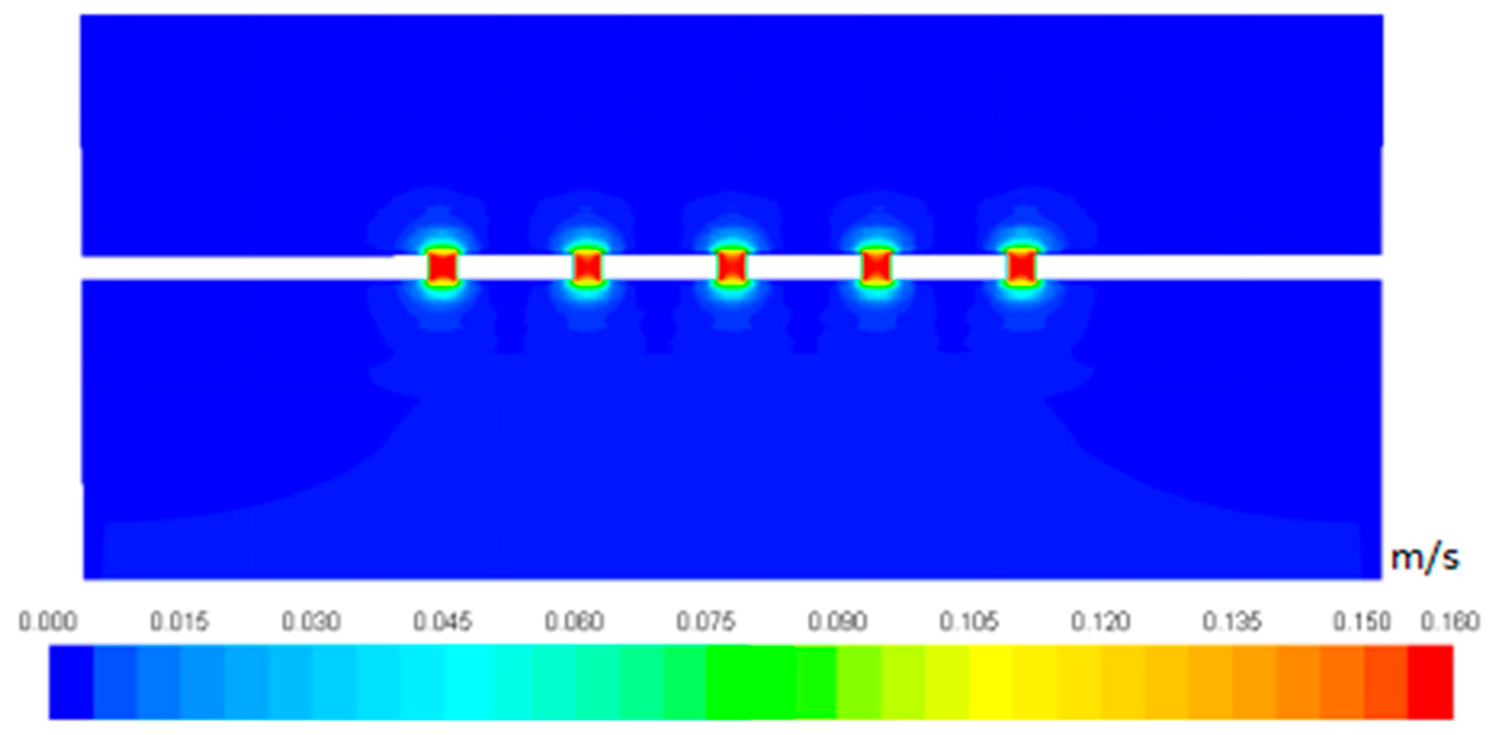
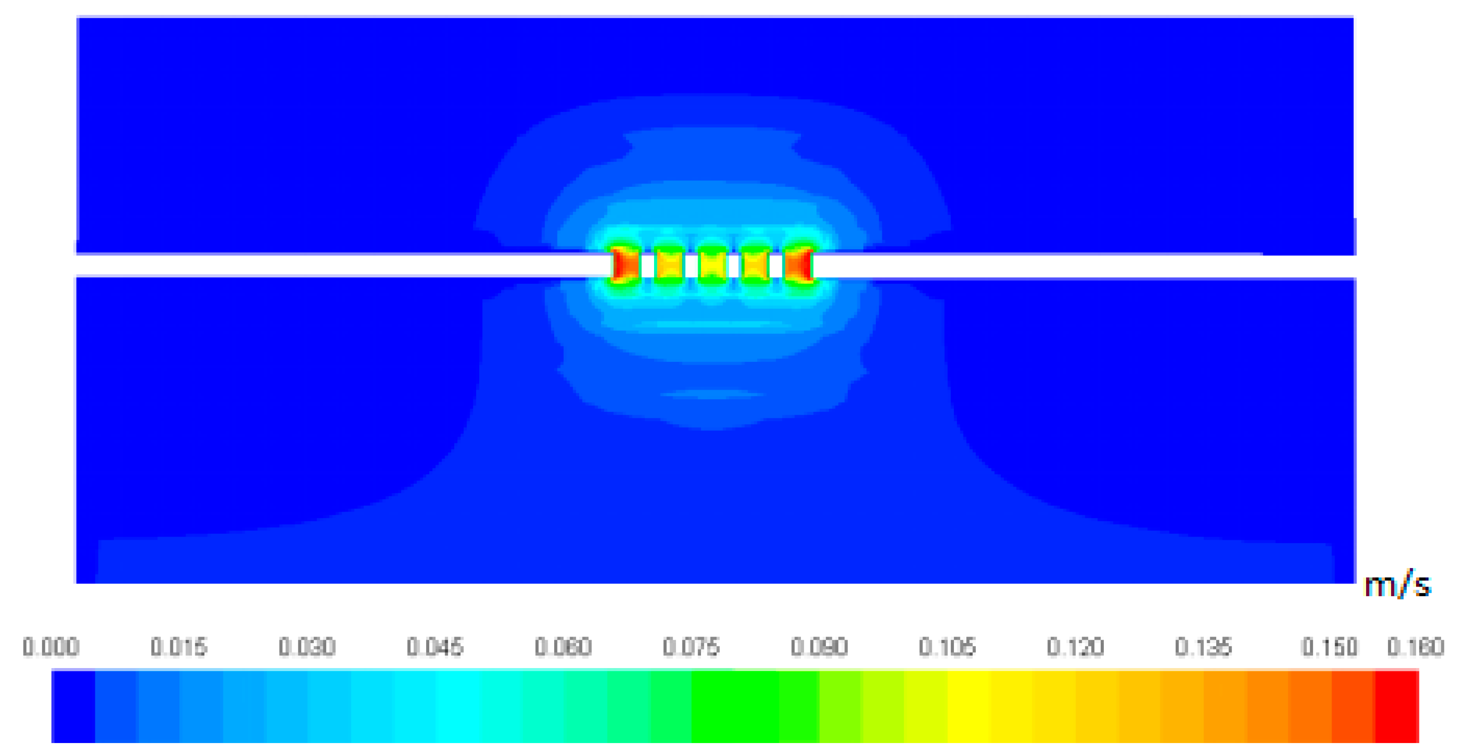
The acoustic velocity magnitude in the vicinity of the perforations is visualized using the results from the CFD simulations of Plate No. 7 with distantly spaced holes, shown in Figure 11, and Plate No. 2 with closely spaced holes, shown in Figure 12. Figure 13 presents a cross-section view of the same holes.

There is a clear indication that when holes are distant from each other, such as those on Plate No. 7 absorber, the oscillating masses for each orifice are so far apart that they barely affect each other. The holes radiate pressure fluctuations separately. By contrast, for plate No. 2, the acoustic velocity does not diminish so rapidly when neighboring holes are very close, due to the combined momentum of the interacting jet flows from neighboring holes. As a result, the strong oscillating mass is sustained further downstream and forms an extra film of what may be considered to be high acoustic velocity, as shown in Figure 12. This gives rise to the extra acoustic radiation effect from the perforation area as a whole to the acoustic downstream space. In this paper, this extra radiation effect is named “acoustic radiation effect due to the overall perforation area”.

From the other perspective, a close hole separation distance (x/d = 1.5) in Plate No. 2 makes the “attached mass” near each individual hole slightly horizontally narrower in comparison with that observed in Plate No. 7 due to hole interaction effect, yet the “attached mass” near each individual hole is somewhat stretched in the vertical direction. However, the “attached mass” near each individual hole can be considered to not be affected to a noticeable degree by acoustic radiations due to the overall perforation area.

Therefore, it may be considered that the end correction due to acoustic radiation for an individual hole is not affected by the acoustic radiation effect, due to the overall perforation area. The acoustic radiation effect from the perforation area as a whole manifests itself by forming an extra acoustic radiation effect in the vicinity of the overall perforated area. The acoustic radiation effect of a perforated plate is treated as a superimposition of two radiation effects: the “individual hole radiation effect” and the “overall perforation region radiation effect”. An acoustic signal experiences the single hole radiation effect and the perforation region radiation effect simultaneously. A simple model is proposed in this paper by assuming that acoustic end correction lengths caused by these effects are additive.

As was introduced earlier, the end correction length due to single hole radiation effect has been analytically derived to be [4,5,6]:

$$l_{sh}=0.96\sqrt{A_0}$$

(13)

Consider an extreme case where all perforations are just next to each other (x/d=1). The orifices nearly work as a single large hole in terms of acoustic radiations. Therefore, it is proposed that acoustic end corrections due to the overall perforation area follow a similar form with that caused by an individual hole.

$$l_{op}=C\cdot 0.96\sqrt{A}$$

(14)

where $A_0$ stands for area of an individual perforation and A is the overall opening area of all orifices. A correcting parameter C is introduced to consider the extent to which the perforation region is acting like a single large hole. C is large when holes are close to each other and it is zero when holes are far away from each other. A simple model is proposed in this paper by assuming that acoustic end correction lengths caused by these effects are additive.

$$l_{ec}=l_{sh}+l_{op}=0.96\sqrt{A_0}+C\cdot 0.96\sqrt{A}$$

(15)

where ${\sigma }_{eff}$ represents the effective porosity of the perforation area; $l_{sh}$ is the end correction length due to acoustic radiation effect near an individual hole and $l_{op}$ stands for the end correction length due to the acoustic radiation effect due to the overall perforation area. C is a factor for the overall perforation area radiation effect. The factor C for all twenty-five numerically investigated PPAs was determined from Equations (1) and (15), as listed in

Table 3. Numerical results of resonance frequencies and end correction lengths for all simulated perforated plates.

Case No. CFD	${\mathit{\sigma }}_{\mathit{e}\mathit{f}\mathit{f}}$	${\mathit{f}}_{\mathit{r}} \left(\mathbf{Hz}\right)$	${\mathit{l}}_{\mathit{e}\mathit{c}} \left(\mathbf{mm}\right)$	C
1	0.545	429	5.562	0.654
2	0.349	457	4.275	0.503
3	0.196	492	2.970	0.349
4	0.126	517	2.194	0.258
5	0.087	535	1.696	0.199
6	0.049	561	1.062	0.125
7	0.031	576	0.721	0.085
8	0.545	373	8.141	0.639
9	0.444	401	6.452	0.506
10	0.250	435	4.512	0.354
11	0.160	461	3.320	0.260
12	0.111	481	2.529	0.198
13	0.063	510	1.544	0.121
14	0.040	530	0.955	0.075
15	0.545	331	11.000	0.647
16	0.444	357	8.764	0.516
17	0.250	392	6.037	0.355
18	0.160	417	4.471	0.263
19	0.111	437	3.411	0.201
20	0.063	470	1.988	0.117
21	0.040	492	1.179	0.069
22	0.105	473	2.721	0.2234
23	0.079	490	2.123	0.1665
24	0.052	508	1.522	0.1194
25	0.039	521	1.136	0.0891

, and then plotted against effective porosities, as presented in Figure 14.

A model relating the overall perforation area radiation effect to the effective porosity was obtained by regression analysis, yielding:

$$l_{op}=0.96\sqrt{A}\cdot \left(0.78\sqrt{{\sigma }_{eff}}-0.11\right)$$

(16)

The total end correction length considering both acoustic radiation effects then becomes:

$$l_{ec}=l_{sh}+l_{op}=0.96\sqrt{A_0}+0.96\sqrt{A}\left(0.78\sqrt{{\sigma }_{eff}}-0.11\right)$$

(17)

The resonant frequency of a distributed Helmholtz resonator

$$f_r=\frac{c}{2\pi }\sqrt{\frac{A}{V{l}_e}}=\frac{c}{2\pi }\sqrt{\frac{A}{V\left(l+l_{ec}\right)}}=\frac{c}{2\pi }\sqrt{\frac{A}{V(l+0.96\sqrt{A_0}+0.96\sqrt{A}\left(0.78\sqrt{{\sigma }_{eff}}-0.11\right)}}$$

(18)

where $l_{ec}$ represents the total end correction length of a PPA, $l_{sh}$ represents end correction length as a result of acoustic radiation effect due to individual perforation, and $l_{op}$ represents end correction length as a result of acoustic radiation effect due to the overall perforation region. The above model was fitted to the available data within an effective porosity range of 3.14–55% and an aspect ratio range of 0.4:1–1:1.

The model provides an overall assessment for the impact of hole interaction effect on acoustic radiation effect by introducing a simple additive term “overall perforation area radiation effect”, under the assumption that acoustic radiation effect from the overall perforation area does not change the end correction length $0.96\sqrt{A_0}$ caused by acoustic radiation from each individual hole.

As shown in Figure 14, the later term $l_{op}$ reduces to zero when ${\sigma }_{eff}\approx 2\%$, which suggests the situations where the holes are far enough away from each other that the perforation area as a whole does form acoustic radiations. In these situations, holes radiate sound separately.

3.2. Validation of the Model

The model, as described earlier in Equations (17) and (18), was determined based on numerical results alone. In this section, the model is validated by comparison with experimental results for eighteen distributed Helmholtz resonators. Effective porosities of these experimentally tested perforated plates range from 0.0436 to 0.4987, porosities of these plates ranges from 0.0338 to 0.135, and perforation aspect ratios range from 1:1 to 1:3.

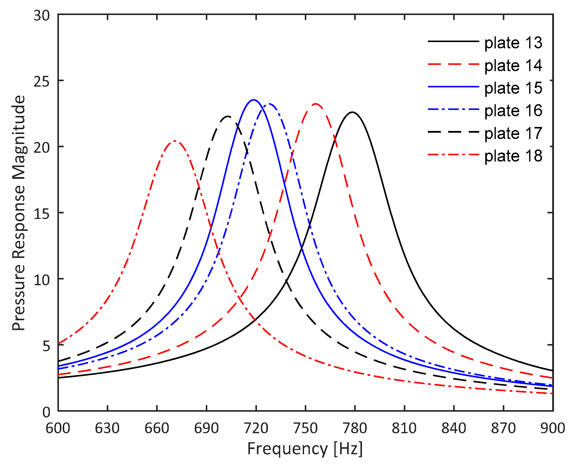
Figure 15, Figure 16 and Figure 17 display the magnitude of pressure response functions between microphone 1 in the resonator and microphone 2 in the acoustic propagation duct. The experimental results suggest that resonance frequencies of PPAs shift to lower frequencies as the holes approach each other. This finding is in agreement with CFD investigations within a wide range of effective porosities from approximately 0.04 to 0.54. This range of 0.04–0.54 covers the effective porosity of most practical PPAs that exhibit a hole–hole acoustic interaction effect. An even lower porosity than 0.04 does not exhibit a noticeable hole–hole interaction effect. A higher effective porosity than 0.54 is not investigated because a PPA with higher effective porosity is nearly a single hole in terms of acoustic radiation effect (for example, for a plate with an effective porosity of 0.6, the ratio of hole diameter (d) to hole center distance (b) is 0.874, which means the orifice is so close that only a distance of 0.126d exists in between their edges).

Resonance frequencies of all eighteen PPAs are determined from Figure 15, Figure 16 and Figure 17 and then listed in

Table 4. Comparison of experimental and fitted model results for end correction lengths.

Case #	${\mathit{\sigma }}_{\mathit{e}\mathit{f}\mathit{f}}$	${\mathit{f}}_{\mathit{r}} \left(\mathbf{Hz}\right)-\mathbf{EXP}$	${\mathit{f}}_{\mathit{r}} \left(\mathbf{Hz}\right)-\mathbf{Model}$	${\mathit{l}}_{\mathit{e}\mathit{c}}$$-\mathit{F}\mathit{o}\mathit{k} \left(\mathbf{mm}\right)$	${\mathit{l}}_{\mathit{e}\mathit{c}}-\mathbf{EXP} \left(\mathbf{mm}\right)$	${\mathit{l}}_{\mathit{e}\mathit{c}}-\mathbf{Model} \left(\mathbf{mm}\right)$	Model Relative Error (%)
1	0.0436	579	595	<1.7 mm	2.45	2.21	−9.80
2	0.0582	573	579	<1.7 mm	2.54	2.45	−3.59
3	0.0873	556	554	<1.7 mm	2.82	2.86	1.18
4	0.0623	563	575	<1.7 mm	2.71	2.51	−7.04
5	0.0831	554	557	<1.7 mm	2.86	2.80	−1.92
6	0.1247	520	531	<1.7 mm	3.52	3.29	−6.41
07	0.0982	683	719	<2.55 mm	5.19	4.49	−13.5
08	0.1309	676	691	<2.55 mm	5.34	5.03	−5.79
09	0.1963	644	649	<2.55 mm	6.09	5.95	−2.34
10	0.1402	650	683	<2.55 mm	5.94	5.18	−12.8
11	0.1870	642	654	<2.55 mm	6.14	5.83	−5.10
12	0.2805	606	613	<2.55 mm	7.14	6.92	−3.02
13	0.1745	778	790	<3.4 mm	7.86	7.55	−3.88
14	0.2327	757	753	<3.4 mm	8.41	8.52	1.31
15	0.3491	719	700	<3.4 mm	9.54	10.15	6.37
16	0.2493	728	744	<3.4 mm	9.26	8.78	−5.20
17	0.3324	703	707	<3.4 mm	10.07	9.93	−1.37
18	0.4987	671	655	<3.4 mm	11.29	11.88	5.21

${\sigma }_{eff}$: Effective porosity; $f_r$ (Hz)-EXP: resonant frequency obtained by experimental method; $f_r$ (Hz)-Model: resonant frequency obtained by the proposed model as given in Equation (18);$l_{ec}$-$Fok$: acoustic end correction length obtained by Fok’s function as given in Equation (4); $l_{ec}$-EXP: acoustic end correction length from experiment; $l_{ec}$-Model: predicted acoustic end correction length by using the proposed model as given in Equation (17).

. Then, the experimental end correction length was calculated by employing Equation (1). End correction lengths acquired by the proposed model (Equation (17)) are similarly provided in Table 4.

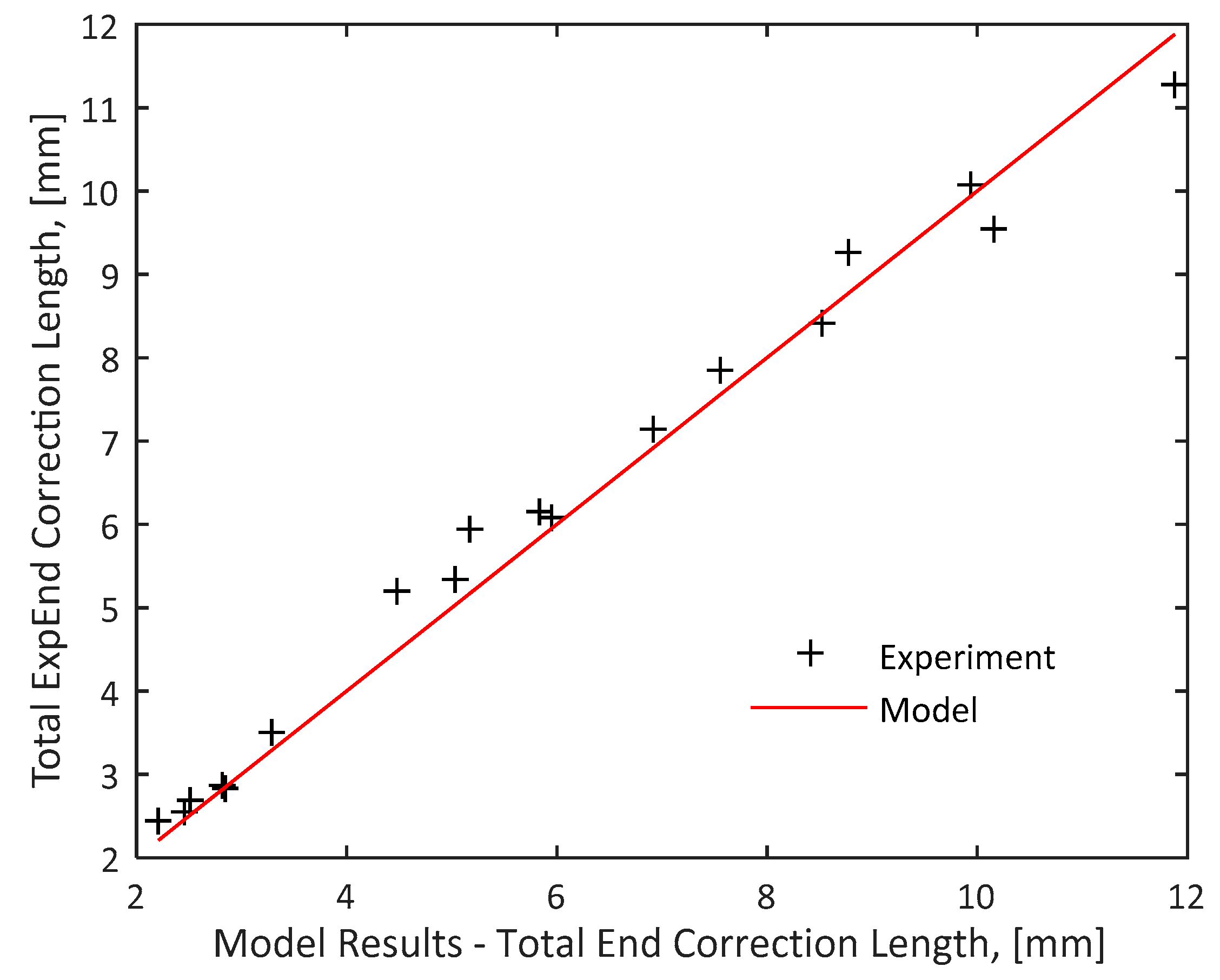
The experimental end correction lengths for all eighteen distributed Helmholtz resonators are plotted against the model results, as shown Figure 18. The figure shows that the proposed model resulting from the regression of the CFD simulation data successfully provides a satisfactory agreement with the experimental results. The relative errors with respect to the experimental results are provided in Table 4 as well. Both experimental results and model results predict an increase of end correction length with closer hole separation distance due to the hole–hole interaction effect. By contrast, as listed in Table 4, predictions according to Fok’s function (Equation 4) always generate end correction lengths less than $0.96\sqrt{A_0}$, which are much lower than experimental results.

On the other hand, as can be seen from the error analysis listed in Table 4, the model tends to slightly underestimate the acoustic end correction length in comparison with some of the experimental data; this model underestimation is more significant for plates with a y = 12 mm, where there are holes very close to cavity walls. As a result, a noticeable hole-to-wall interaction effect will probably contribute to the error.

4. Conclusions

A model for the prediction of resonance frequencies of distributed Helmholtz resonators is proposed. The model was initially derived based on high resolution computational simulations for twenty-five distributed Helmholtz resonators. End correction length was proposed to be correlated with two acoustic radiation effects, namely, acoustic radiation effect from the individual hole and acoustic radiation from the overall perforation area. The model was then acquired by making a convenient assumption that the end correction lengths due to these two acoustic radiation effects are additive. It is noteworthy that the assumption is not strictly validated analytically, as its purpose is to make the model easy to use in practice.

The proposed resonant frequency model was successfully validated by comparison with experimental data for a further eighteen distributed Helmholtz resonators. The validation exercise demonstrated that the proposed model displays very good agreement with the experimental results for resonance frequencies for distributed Helmholtz resonators within a wide range of effective porosities (0.04–0.54), porosities (0.0123–0.135), and perforation aspect ratios (1:1–1:3). A new term, “overall perforation area acoustic radiation effect”, is proposed to account for the acoustic radiations from the perforated area as a whole.

This resulting model is easily applicable for engineers and is of significant value in the design of practical distributed Helmholtz resonators, such as those distributed Helmholtz resonators applied on gas turbine engines to control combustion instabilities.

References

- Elsa Gullaud, F.N. Effect of Perforated Plates on the Acoustics of Annular Combustors. AIAA J. 2012, 50, 2629–2642. [Google Scholar] [CrossRef]
- Lahiri, C. Acoustic Performance of Bias Flow Liners in Gas Turbine Combustors. Ph.D. Thesis, Technische Universität Berlin, Berlin, Germany, 2014. [Google Scholar]
- Noiray, N.; Durox, D.; Schuller, T.; Candel, S. Passive control of combustion instabilities involving premixed flames anchored on perforated plates. Proc. Combust. Inst. 2007, 31, 1283–1290. [Google Scholar] [CrossRef]
- Kuttruff, H. Acoustics: An Introduction; CRC Press: Boca Raton, FL, USA, 2007. [Google Scholar]
- Ingard, U. On the theory and design of acoustic resonators. J. Acoust. Soc. Am. 1953, 25, 1037–1061. [Google Scholar] [CrossRef]
- Bolt, R.H.; Labate, S.; Ingård, U. The acoustic reactance of small circular orifices. J. Acoust. Soc. Am. 1949, 21, 94–97. [Google Scholar] [CrossRef]
- Rayleigh, L. Theory of Sound; Macmillan: London, UK, 1940. [Google Scholar]
- Fok, B.M.W. Theoretical study of the conductance of a circular hole in a partition across a tube. Dokl. Akad. Nauk SSSR 1941, 31, 875–882. [Google Scholar]
- Atalla, N.; Sgard, F. Modeling of perforated plates and screens using rigid frame porous models. J. Sound Vib. 2007, 303, 195–208. [Google Scholar] [CrossRef]
- Melling, T.H. The acoustic impedance of perforates at medium and high sound pressure levels. J. Sound Vib. 1973, 29, 1–65. [Google Scholar] [CrossRef]
- Randeberg, R.T. Perforated Panel Absorbers with Viscous Energy Dissipation Enhanced by Orifice Design. Ph.D. Thesis, Norwegian University of Science and Technology, Trondheim, Norway, 2000. [Google Scholar]
- Rzhevkin, S.N. A Course of Lectures on the Theory of Sound; Pergamon Press: Oxford, UK, 1963. [Google Scholar]
- Sobolev, A.F. A semiempirical theory of a one-layer cellular sound-absorbing lining with a perforated face panel. Acoust. Phys. 2007, 53, 762–771. [Google Scholar] [CrossRef]
- Tayong, R. On the holes interaction and heterogeneity distribution effects on the acoustic properties of air-cavity backed perforated plates. Appl. Acoust. 2013, 74, 1492–1498. [Google Scholar] [CrossRef]
- Tayong, R.; Dupont, T.; Leclaire, P. Experimental investigation of holes interaction effect on the sound absorption coefficient of micro-perforated panels under high and medium sound levels. Appl. Acoust. 2011, 72, 777–784. [Google Scholar] [CrossRef] [Green Version]
- Bolton, J.S.; Kim, N. Use of CFD to calculate the dynamic resistive end correction for microperforated materials. Acoust. Aust. 2010, 38, 134–139. [Google Scholar]
- Temiz, M.A.; Lopez Arteaga, I.; Efraimsson, G.; Hirschberg, A. The influence of edge geometry on end-coefficients in micro perforated plates. J. Acoust. Soc. Am. 2015, 138, 3668–3677. [Google Scholar] [CrossRef] [PubMed]
- Li, X. End correction for the transfer impedance of microperforated panels using viscothermal wave theory. J. Acoust. Soc. Am. 2017, 141, 1426–1436. [Google Scholar] [CrossRef] [PubMed]
- Wang, J.; Rubini, P.; Qin, Q. Application of a porous media model for the acoustic damping of perforated plate absorbers. Appl. Acoust. 2017, 127, 324–335. [Google Scholar] [CrossRef]
- Fluent, A. 12.0 Theory Guide. Chapter 21: Solver Theory; ANSYS, Inc.: Southpointe, PA, USA, 2009. [Google Scholar]
- Poinsot, T.J.; Lelef, S.K. Boundary conditions for direct simulations of compressible viscous flows. J. Comput. Phys. 1992, 101, 104–129. [Google Scholar] [CrossRef]
- Selle, L.; Nicoud, F.; Poinsot, T. Actual impedance of nonreflecting boundary conditions: Implications for computation of resonators. AIAA J. 2004, 42, 958–964. [Google Scholar] [CrossRef]
- Seybert, A.F.; Ross, D.F. Experimental determination of acoustic properties using a two microphone random-excitation technique. J. Acoust. Soc. Am. 1977, 61, 1362–1370. [Google Scholar] [CrossRef]
Figure 1.
Fok’s function.
Figure 2.
Illustration of the Hole–Hole interaction effect, redrawn, based upon Melling [10].
Figure 3.
An impedance tube configured with two microphones.
Figure 4.
An example of six perforated plate configurations.
Figure 5.
Grid resolution in an impedance tube configured with plate No. 7 absorber: (a) grid resolution in the test rig and (b) grid resolution in the hole (Hole Diameter = 2 mm).
Figure 6.
Normalized specific acoustic impedance of perforated plate No. 7 absorber acquired by 0.1 mm and 0.2 mm resolution computational grids in the hole.
Figure 7.
Experimental Test Rig Setup.
Figure 8.
The position and shape of the distributed Helmholtz resonator on the experimental test rig.
Figure 9.
Orifice separation distances (mm) in different directions of tested perforated plates 1–6.
Figure 10.
CFD obtained resonance frequencies of perforated plate No. 1–25 absorbers (as listed in Table 1).
Figure 11.
Acoustic velocity magnitude contour near perforated plate No. 7 absorber.
Figure 12.
Acoustic velocity magnitude contour near perforated plate No. 2 absorber.
Figure 13.
Acoustic velocity magnitude contour near an orifice with different hole separation distance: (a) plate No.7 absorber: x/d = 5, y/d = 5, (b) plate No.2 absorber: x/d = 1.5, y/d = 1.5.
Figure 14.
Proposed model for end correction factor as a function of effective porosity.
Figure 15.
Experimental pressure response functions for plate 1 to plate 6.
Figure 16.
Experimental pressure response functions for plate 7 to plate 12.
Figure 17.
Experimental pressure response functions for plate 13 to plate 18.
Figure 18.
Validation of the proposed model against experimental results. (—: model results, +: experiment results).