Unsupervised Novelty Detection Using Deep Autoencoders with Density Based Clustering


1
Database and Bioinformatics Laboratory, School of Electrical and Computer Engineering, Chungbuk National University, Cheongju 28644, Korea
2
Faculty of Information Technology, Ton Duc Thang University, Ho Chi Minh City 700000, Vietnam
*
Author to whom correspondence should be addressed.
Appl. Sci. 2018, 8(9), 1468; https://doi.org/10.3390/app8091468
Submission received: 30 July 2018
/
Revised: 21 August 2018
/
Accepted: 22 August 2018
/
Published: 27 August 2018
(This article belongs to the Special Issue Deep Learning and Big Data in Healthcare)
Abstract
:Novelty detection is a classification problem to identify abnormal patterns; therefore, it is an important task for applications such as fraud detection, fault diagnosis and disease detection. However, when there is no label that indicates normal and abnormal data, it will need expensive domain and professional knowledge, so an unsupervised novelty detection approach will be used. On the other hand, nowadays, using novelty detection on high dimensional data is a big challenge and previous research suggests approaches based on principal component analysis (PCA) and an autoencoder in order to reduce dimensionality. In this paper, we propose deep autoencoders with density based clustering (DAE-DBC); this approach calculates compressed data and error threshold from deep autoencoder model, sending the results to a density based cluster. Points that are not involved in any groups are not considered a novelty; the grouping points will be defined as a novelty group depending on the ratio of the points exceeding the error threshold. We have conducted the experiment by substituting components to show that the components of the proposed method together are more effective. As a result of the experiment, the DAE-DBC approach is more efficient; its area under the curve (AUC) is shown to be 13.5 percent higher than state-of-the-art algorithms and other versions of the proposed method that we have demonstrated.
1. Introduction
An abnormal pattern that is not compatible with most of the data in a dataset is named a novelty, outlier, or anomaly [1]. Novelty can be created for several reasons, such as data from different classes, natural variation and data measurement or collection errors [2]. Although there may be novelty due to some mistakes, sometimes it is a new, unidentified process [3]; therefore, it is useful to discover important information by detecting the novelty in a variety of application domains such as internet traffic detection [4,5], medical diagnosis [6], fraud detection [7], traffic flow forecasting [8] and patient monitoring [9,10].
There are three basic ways to detect novelty depending on the availability of data label [1]. If the data is labeled as normal or novelty, a supervised approach can be used as a traditional classification task. In this case, training data consists of both normal and novelty data and builds a model that predicts unseen data as normal and novelty. However, novelty faces with a class imbalance problem due to the relatively low comparability of normal data [11]. Also, obtaining an accurate labeling for abnormal data is transformed into a complex problem in data size and high dimension. The second method is a semi-supervised method, which only uses normal data to build a classification model. If the training data contains abnormal data, the model may find it difficult to detect the abnormal data. Moreover, most of the data are not labeled in the practice, and in this case, an unsupervised method, such as the third, is used.
In recent years, research related to unsupervised novelty detection suggest using One-class Support Vector Machine (OC-SVM) based, clustering based, reconstruction error based methods and to combine these methods together.
OC-SVM separates normal and novelty data as projecting the input features into the high dimensional feature spaces using a kernel trick. In other words, finding the decision boundary that the farthest isolate the origin and data points and the closest points to the origin considered as the novelty. However, SVM is a memory and time-consuming task in practice and its complexity grows quadratically with the number of records [12].
Cluster analysis divides data into groups that are meaningful, useful, or both [2]. In clustering based novelty detection, there are several ways to identify novelty, such as clusters that are located far away from other clusters, or smaller or sparser than other clusters, or points not belonging to any group are considered as abnormal data. But the cluster-based method performance is very dependent on which algorithm is used as well as high-dimensional data in clustering with distance is special challenges to data mining algorithms [13].
To address this issue caused by the curse of dimensionality, reconstruction error based approach and hybrid approaches are widely used. PCA is a technique used to reduce dimensionality. Peter J. Rousseeuw and Mia Hubert introduced diagnosis of anomalies by the first principal component score and its orthogonal distance to each data point [14]. Heiko Hoffmann introduced kernel PCA (KPCA), which maps input spaces into higher-dimensional space before performing the PCA using a kernel function for outlier detection [15]. In a hybrid approach, dimensionality reduction first made and then clustering or other classification algorithms are performed in the latent low-dimensional space. In recent publications, unsupervised novelty detection using deep learning is proven by high effectiveness [3,12,16,17,18]. They use an autoencoder that is an artificial neural network to extract features and to reduce the dimension then give them as an input to the novelty identification methods such as Gaussian mixture model, cumulative distribution function and clustering algorithm and so on.
In this paper, the DAE-DBC method is suggested and aims to increase the accuracy of unsupervised novelty detection. First, use a deep autoencoder model to extract a low dimensional representation from the high dimensional input space. The architecture of the autoencoder model consists of two symmetrical deep neural networks—an encoder and a decoder that applies backpropagation, setting the target values to be equal to the inputs. It attempts to copy its input to its output and anomalies are harder to reconstruct compared with normal samples [16]. In DAE-DBC, low dimensional representation of data includes bottleneck hidden layer in autoencoder network and reconstruction error of each point. Based on reconstruction error, we estimate the first outlier threshold and distinguish data is normal or abnormal using it. But in this step, data cannot be divided clearly. Then, the autoencoder model is retrained only with normal data and low dimensional representation and optimal outlier threshold are calculated again using by the retrained model. The low dimensional data from retrained autoencoder model is classified into groups using the Density-based spatial clustering of applications with noise (DBSCAN) clustering algorithm. The optimal value of eps parameter (minimum distance between two points) of DBSCAN is estimated by DMDBSCAN algorithm [19]. Based on the optimal outlier threshold from retrained autoencoder model, identify novelty. If most of the instances in a group exceed our threshold, all instances in this cluster are considered as abnormal and labeled by novelty. We have tested DAE-DBC on several public benchmark datasets, it presents higher AUC score than the state-of-the-art techniques.
We propose the unsupervised novelty detection method over high dimensional data based on deep autoencoder and density-based clustering. The main contribution of the proposed method are as follows:
- We derive a new DAE-DBC method for unsupervised novelty detection that is not domain specific.
- The number of clusters is unlimited and each cluster will be labeled by novelty depending on what percentage of objects that it contains exceed the error threshold. In other words, identifying novelty is based on the reconstruction error threshold without considering the sparse, or far, or small ones. Therefore, large-scale clusters are also possible to be novelty.
- Our extensive experiment shows that DAE-DBC has a greater performance than other state-of-the-art unsupervised anomaly detection methods.
This article consists of 5 sections. In Section 2, we provide a detailed survey of related work on unsupervised anomaly detection. Our proposed method is explained in Section 3. Section 4 presents the experimental dataset, compared methods, the evaluation metric and the result and comparison of experiments. Finally, Section 5 concludes the paper.
2. Related Work
In this section, we have introduced an unsupervised novelty detection method related to the proposed method. Recent research suggests unsupervised techniques, such as OC-SVM, one-class neural network (OC-NN), clustering based and reconstruction error based and so on.
The relatively small percentage of total data is novelty and class imbalance problems can occur because of divergence of normal and novelty sample ratios. In this case, traditional classification methods are not well suited for discovering novelty. OC-SVM is the semi-supervised approach that is used for a classifier based on building a prediction model from a normal dataset [20,21,22,23]. It is an extension of SVM for an unlabeled dataset that was introduced first by Schölkopf et al. [23] and usage of one-class SVM in unsupervised mode is rising due to the most data is not labeled in the practice. In this case, all data is considered normal and used for the training of OC-SVM. The disadvantage of this method is that if the training data contains abnormal or novelty, the novelty detection classification model does not work well because the decision boundary (the normal boundary) created by OC-SVM shifts toward outliers.
Mennatallah et al. showed an Enhanced OC-SVM which is the Robust OC-SVM and the eta-SVM together to eliminate these deficiencies [20]. Robust OC-SVM focused on slack variables that are far from the centroid. They are dropped from the minimization objective because of these points, the decision boundary will be wrong. Sarah M. Erfani et al. proposed a hybrid model that combines a deep belief network for feature extraction and OC-SVM for unsupervised novelty detection—named DBN-1SVM—that solves the curse of the dimensionality problem by reducing dimensionality using a deep belief network [12].
Another popular novelty detection method is principal component analysis (PCA) based methods. PCA is a dimension reduction technique in which the direction with the largest projected variance is called the first principal component. The orthogonal direction that captures the second largest projected variance is called the second principal component and so on [24]. Although in most cases, PCA is used for dimensionality reduction purpose, it is also used to detect novelty. Peter J. Rousseeuw et al. introduced to diagnose outliers by the first principal component score and its orthogonal distance of each data points. Regular observations have both a small orthogonal distance and small PCA score [14]. Heiko Hoffman proposes kernel PCA for novelty detection which is a non-linear extension of PCA. In kernel PCA, input spaces are mapped into higher-dimensional space before performing PCA using a kernel function. In Heiko Hoffman’s proposed method, Gaussian kernel function and reconstruction error in feature space are used [15]. Using the covariance matrix to PCA is sensitive to the outlier. Roland Kwitt et al. proposed a Robust PCA based novelty detection approach using the correlation matrix instead of the covariance matrix to calculate the principal component scores [25].
In recent studies, hybrid techniques are being suggested that making novelty detection as a deep autoencoder is combined with other methods. Deep autoencoder is a neural network that is trained to attempt to copy its input to its output. Yu-Dong Zhang et al. proposed a deep neural network with seven layers for voxelwise detection of cerebral microbleeds. They used sparse autoencoder with 4 hidden layers for dimensionality reduction and softmax layer for classification [26]. Also, Wenjuan Jia et al. proposed a deep stacked autoencoder based multi-class classification approach to the image dataset. The first dimensionality is reduced using deep stacked autoencoder and then softmax layer is used as a classifier [27]. Yan Xia et al. propose a reconstruction based outlier detection method that has 2 steps including discriminative labeling and reconstruction learning [28]. They show that dataset reconstructed from low-dimensional representations, the inliers and the outliers can be well separated according to their reconstruction error. Hyunsoo Kim et al. propose an unsupervised land classification system using quaternion autoencoder for feature extraction and self-organizing map (SOM) for classification without human-predefined categories [18]. Bo Zong et al. introduce a technique that combines the deep autoencoder model with the Gaussian mixture model—named the DAGMM algorithm. DAGMM identifies novelty by providing inputs of Gaussian mixture model by the outcome of deep autoencoder model which is low dimensional features and reconstruction errors [16].
3. Methodology
In this section, we have amplified how to describe the novelty detection of data without labels using a deep learning autoencoder (AE) reconstruction error.
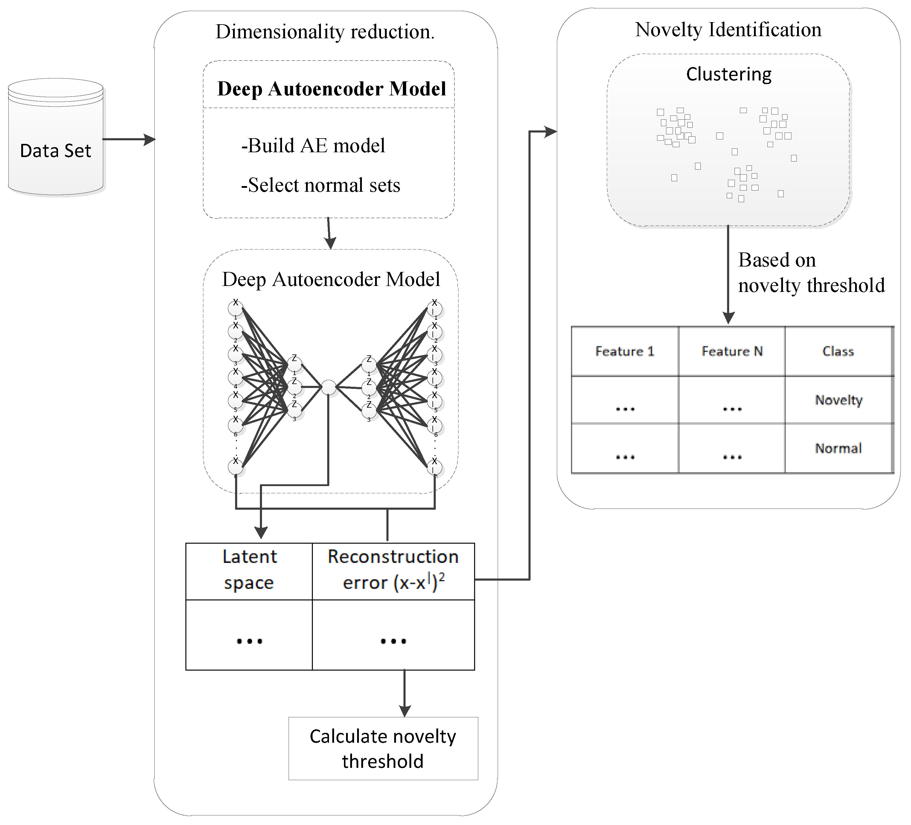
The proposed approach has two basic functions: dimension reduction and identification of novelty. The general architecture of the proposed method is illustrated in Figure 1:
3.1. Deep Autoencoders for Dimensionality Reduction
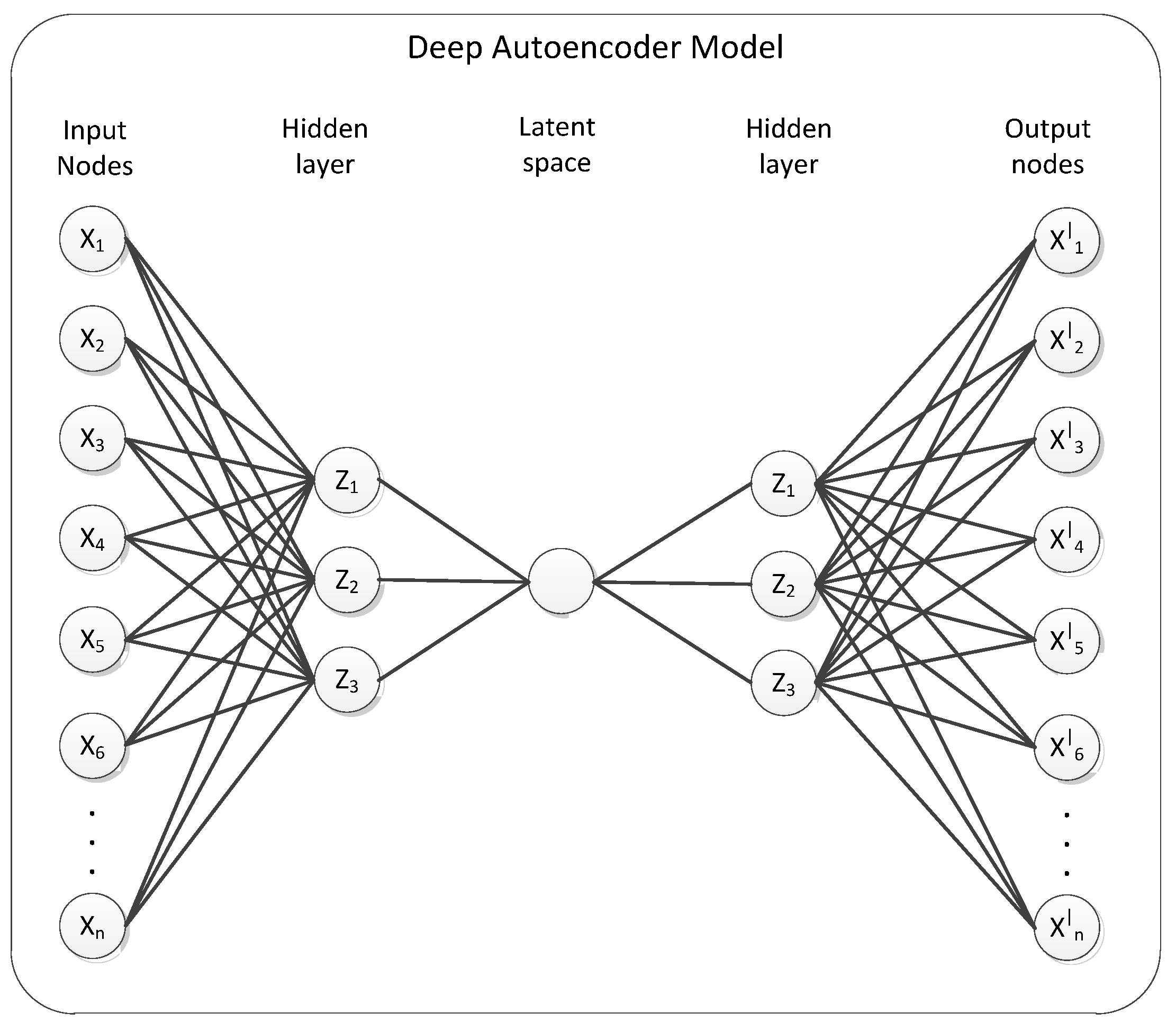
Autoencoder is one kind of ANN [28], which is the unsupervised algorithm for learning to copy its own input (x1 … xn) to its output (y1 … yn) as close (xi = yi) as possible by reducing the gap between inputs and outputs [29]. As visualized in Figure 2, input and output neurons are the same for AE and its hidden layer is a compressed or learned feature. In general, the AE structure is the same as a neural network with a hidden layer at least 1 but AE is distinguished from the goal to predict the output corresponding to the specific input of NN by the purpose of reconstruct the input. The learning process of AE first compress input x to a small dimension and reconstruct an output y from the small dimension and calculates the difference between the input and reconstructed values and changes weight assignments to reduce the difference. As the novelty data, the reconstruction error is high due to the lack of successful reconstruction of the low-dimensional projection.
In the research work, the compressed representation of data provided by deep AE contains two features (1) reduced dimensional representation and (2) the reconstruction error from input and reconstructed features by learned deep autoencoder model. As shown in Figure 1, there are two AE models are used to estimate the novelty threshold and compressed representation of data. From the first AE model, the initial novelty threshold will be calculated. After that, we get rid of data that close to the normal using this threshold and the second AE model is trained by these data. To estimate the optimal threshold from the distribution histogram of the reconstruction error commonly used thresholding technique, the Otsu method [30] is used. The Otsu method calculates the optimum threshold by separating the two classes. Therefore, the desired threshold corresponds to the maximum value of between two class variances. Get the best-suited error threshold for separating novelty and normal values because of the second model trained by data close to the norms. We calculate the final compressed data that is composed of a reconstruction error and reduced dimensional representation by giving again all inputs to the second AE model. Algorithm 1 shows the Dimensionality reduction which is one of the two basic functions of the proposed method step by step:
| Algorithm 1: Dimensionality reduction. |
| 1: Input: Set of points 2: Output: Z |
| 3: inputLayer ← ( n_ nodes = n) 4: encoderLayer1 ← Dense(n_ nodes = n/2, activation = sigmoid)(inputLayer) 5: encoderLayer2 ← Dense(n_ nodes = 1, activation = sigmoid)(encoderLayer1) 6: decoderLayer1 ← Dense(n_ nodes = n/2, activation = tanh)(encoderLayer2) 7: decoder _layer2 ← Dense(n_ nodes = n, activation = tanh)(decoderLayer1) 8: AEModel ← Model(input_layer, decoder _layer2) 9: AEModel.fit(X) 10: ← AEModel.predict(X) |
| 11: reconstructionError ← [] 12: for i=0 to do 13: reconstructionErrori ← 2 14: end for |
| 15: threshold ← Otsu(reconstructionError) 16: X[reconstructionError] ← reconstructionError |
| 17: norms ← (X [reconstructionrError] < threshold) |
| 18: AEModel.fit(norms) 19: ← AEModel.predict(X) 20: E ← AEModel. encoderLayer2 |
| 21: reconstructionError ← [] 22: for i to do 23: reconstructionErrori ← 2 24: end for |
| 25: finalThreshold ← Otsu(reconstructionError) |
| 26: Z ← [] 27: Z[encoded] ← E 28: Z[error] ← reconstructionError 29: return Z |
The dimension of each benchmark dataset is varying. Our AE model will be built like that if the dimension of the dataset is n, reduced from dimension n to n/2, from dimension n/2 to 1 and then reconstruct from the reduced dimension by reverting from 1 to n/2, from n/2 to n. Take two-dimensional new data to combine the bottleneck hidden layer which has only 1 node and reconstruction error of each point from this AE model. This new dataset is used by input for further processes for novelty detection. Algorithm 1’s computational complexity is defined as follows:
- Run-time complexity of backpropagation of autoencoder model is O(epochs*training example*(number of weights))
- Prediction process is O(n)
- Calculate reconstruction errors from decoded output and input is O(n)
- Calculate novelty threshold is O(n)
3.2. Density Based Clustering for Novelty Detection
Density-based clustering locates regions of high density that are separated from one another by regions of low density [2]. DBSCAN [31] is a basic, simple and effective density-based clustering algorithm and it can find arbitrarily shaped clusters. In this algorithm, a user specifies two parameters eps which determine a maximum radius of the neighborhood and minPts which determine a minimum number of points in the eps of point.
To automatically adjust the value of the eps parameter, we used the K-dist plot method [31] to calculate the nearest neighboring space for each point. The main idea is that if the point is contained in any cluster, its K-dist value is less than the size of the cluster and in the absence of any cluster, the value of K-dist will be high. Therefore, we have calculated the K-dist value for all points and placed it in ascending order and have chosen the optimal eps for the initial maximum change.
When grouping the data via DBSCAN clustering algorithm, some points do not remain a part of any cluster. In the proposed method, we have considered data points which do not include any clusters as one whole cluster. After grouping of extracted low dimensional feature space (2D), find out which clusters are the novelty. DBSCAN algorithm cannot provide a degree of novelty score [32]. So, we use a final error threshold obtained from the second AE model to make a novelty detection. If the majority of instances of the cluster exceed the threshold, the whole cluster is considered a novelty. Algorithm 2’s computational complexity is defined as:
- Calculate nearest neighbors is O(dn3) where d is dimension and n is the number of samples
- DBSCAN clustering is O(n2)
- Identify novelty is O(n)
In Algorithm 2 shows how to discover novelty step by step:
| Algorithm 2: Identify novelty. |
| 1: Input: Set of points , set op points X, 2: Output: X, #with decision |
| 3: nbrs ← NearestNeighbors (n_neighbors=3).fit (Z) 4: distance ← nbrs.kneighbors (Z) 5: distance.sort() 6: eps ← first extreme value of distance |
| 7: cluster ← dbscan(Z, eps) 8: n_clusters ← len(cluster.labels_) 9: X[labels] ← cluster.labels_ |
| 10: dict_error ← {} 11: for i=0 to n_clusters do 12: bool_values ← (X [labels_] == i ) 13: cluster_i_set ← Z[boolvalues] 14: n_instance_in_cluster_i = len(cluster_i_set) 15: error_count = 0 16: for j in n_instance_in_cluster_i do 17: if cluster_i_set[j] > final_threshold 18: error_count ← error_count + 1 19: endif 20: end for 21: dict_error[i] ← error_count 22: end for 23: for i=0 to n_clusters do 24: cluster_i ← X[db_labels == i] 25: n_of_instance ← len(cluster_i) 26: if n_of_instance * 0.5 less than or equal to dict_error.get(i) 27: X.update[ all rows in cluster, labels ] = 1 #novelty 28: else 29: X. update[ all rows in cluster, labels ] = 0 #normal 30: endif 31: end for 32: return X |
We have summarized the general architecture solutions in Algorithm 3 and the dimensionality reduction and have identified the novelties that are contained in it, which have been summarized in Algorithms 1 and 2.
The generic functions of the proposed DAE-DBC are shown in Algorithm 3:
| Algorithm 3: DAE-DBC algorithm. |
| 1: Input: Set of points 2: Output: Y, { #decision |
| 3: Z ← Dimensionality reduction(X) 4: Y ← Identify novelty(Z) 5: return Y |
High-dimensional data can cause problems for data mining and analysis [24]; also, this curse of dimensionality problem introduced by R. Bellman [33]. To avoid this problem, we have proposed a method instead of grouping directly the input data, to group the low dimensional representation of the input.
The advantage of the proposed method is that by calculating the error threshold in two stages, making it more precise novelty detection. First, the autoencoder model is trained by all data and the first threshold is estimated from its reconstruction error. In this case, using all the data including both the novelty and the normal to train the autoencoder model, so using directly this threshold may have a negative effect on novelty detection. Therefore, according to the estimated threshold, it can get rid of the data which is close to the normal and retrain the autoencoder model using close to normal data. The second model that trained from the data including less number of the novelty than the first one, thus, it is used to estimate the final error threshold and to reduce the dimensionality. Creating clusters from final low dimensional space, to determine whether the cluster is the novelty if the most of instance in a group is abnormal, this cluster is considered as the novelty and labeled by abnormal.
4. Experimental Study
In this section, we have compared the results of our DAE-DBC method, OC-SVM, eta-SVM, Robust-SVM [20], PCA with Gaussian Mixture Model (GMM), PCA with Cumulative distribution function (CDF), kernel PCA with GMM, kernel PCA with CDF, Robust PCA [25] and have proposed method versions that replace its some components by PCA or kernel PCA or K-means clustering technique.
4.1. Datasets
Our outlier benchmark datasets are from the Outlier Detection Datasets (ODDS) website [34]. The original version of benchmark datasets with the ground truth are for a classification in the UCI machine learning repository. The description and class labels that are considered as the novelty of the benchmark datasets in this experiment are detailed in Table 1.
4.2. Methods Compared
We have compared our DAE-DBC which is deep autoencoder reconstruction error based method with the unsupervised state-of-the-art methods below.
- OC-SVM. OC-SVM is used for novelty detection based on building prediction model from only normal dataset [23]. Eta-SVM and Robust SVM that an enhanced OC-SVM are introduced by Mennatallah et al. [20] and they suggest an implementation which is an extension of Rapidminer. We use this extension configured by RBF kernel function for these three algorithms.
- PCA based methods. PCA is commonly used for outlier detection and calculates the outlier score using the principal component scores and reconstruction error which is the orthogonal distance of each data point and its first principal component score. The Gaussian Mixture Model and Cumulative Distribution Function are used to make novelty detection decision from Outlier score [35,36]. We compare the PCA-based methods including PCA-GMM, PCA-CDF, Kernel PCA-GMM, Kernel PCA-CDF and Robust PCA [25].
We present a series of proposed methods by modifying the components to show that the components of the proposed DAE-DBC method together are more effective. In other words, we have tested with some methods, such as the proposed approach with K-means, proposed approach with PCA and proposed approach with KPCA.
- DAE-DBC (Proposed method). The structure of the deep autoencoder is composed of the 5 number of layers like {input layer (n neurons) → encoding layer (n/2 neurons) → encoding layer (1 neuron) → decoding layer (n/2 neurons) → decoding layer (n neuron)}, where n is the number of neurons. In here, the number of neurons in a bottleneck hidden layer which is the compressed representation of the original input is equal to one, other hidden layers are composed of neurons of about a half of the input neurons. The sigmoid activation function is used for encoding type-layers, the tanh activation function is for decoding-type layers respectively. Reconstruction error and compressed representation are grouped by density-based DBSCAN clustering algorithm and the novelty threshold will decide whether the group is the novelty.
- DAE-Kmeans. Compare with the proposed method using the K-means clustering algorithm instead of density-based clustering. K-means clustering algorithms require the number of cluster k and we have used Silhouettes analysis which is used for evaluation of clustering validity to find optimal k [37].
- PCA-DBC, KPCA-DBC. Our proposed method is based on reconstruction error. So, we have used PCA and KPCA in place of AE for calculating reconstruction error and compressed representation.
4.3. Evaluation Metrics
The grand-truth label is used to measure the performance of all the methods used in the experiment. The Receiver Operating Characteristic (ROC) curve and its area under curve (AUC) is used to measure the accuracy of all test methods. AUC represents a summary measure of accuracy and high AUC indicates the good result.
4.4. Experimental Result
The experiment was carried out on a Thinkpad W510, 1st gen i7 and 8GB Ram. First, we have made an experiment on 20 benchmark datasets to compare Algorithm 1 and Algorithm 3. As a result of applying Algorithm 1, we get 2 dimensional features consisting of the reduced dimension and the reconstruction errors as well as a finalThreshold which represents the novelty threshold. If algorithm 1 is used without algorithm 2, each point that is exceeding the finalThreshold will be defined as a novelty. However, the synergy of using both algorithm 1 and algorithm 2 will result in grouping points that exceed the finalThreshold as a novelty group. Table 2 shows that the AUC score of novelty detection is growing when using Algorithm 1 and Algorithm 2 together (Algorithm 3) instead of using Algorithm 1 alone.
Second, we have made experiments on a total of 20 benchmark datasets to compare our proposed algorithms with state-of-the-art algorithms. Extensions of RapidMiner, which is proposed by OC-SVM, eta-SVM, Robust SVM and Robust PCA Mennatallah et al. was used and other algorithms were implemented in Python with Keras, which is a high-level neural networks API, written in Python and capable of running on top of TensorFlow. The Deep autoencoder model is set to match the same for DAE-DBC and DAE-Kmeans algorithms. Deep autoencoder was trained by the Adam algorithm [38] and learning rate was 0.001 to minimize mean squared error. Batch size was 2 and number of epochs to train model was 50.
In implementation of algorithm 1, original CSV data file is loaded into DataFrame in pandas Python package. DataFrame is a 2-dimensional labeled data structure with columns of potentially different types. After building first autoencoder model, decoded output result and reconstruction errors are stored in one-dimensional arrays. The data with a lower reconstruction error is stored into new DataFrame. Train the 2nd autoencoder model by the data obtained and the final compressed data including reconstruction errors and low dimensional representation from second AE model is written into CSV file. In the implementation of algorithm 2, the compressed data file is loaded into the DataFrame. Clusters’ labels and distances between points in the compressed representation are stored in one-dimensional arrays. Also, the count of the novelty in each cluster is stored in a dictionary data structure. The final novelty labels will be appended into the original CSV data file.
Experimental results show that we can use the DAE-DBC method on various dimensions of data due to the fact that it has given higher AUC than other methods on most of the data. A total of 13 methods were tested on 20 benchmark datasets, the highest values of AUC scores are marked in bold in Table 3. The first is the DAE-DBC algorithm 0.7829, the second is the PCA-DBC algorithm 0.6924, the third is OC-SVM algorithm 0.6865 by the average AUC score are higher than other algorithms. The proposed DAE-DBC method shows the AUC score of less than 0.8 on Vertebral, Optdigits, Letter, Arrhythmia and Annthyroid datasets. Comparing the above datasets with the datasets shown in the high AUC score, the average values between some of the features have high variance. Testing 13 methods have sometimes indicated memory errors in KPCA-CDF, KPCA-GMM and KPCA-DBC algorithms depending on sample number. For our proposed DAE-DBC algorithm, all of the data has been successfully tested.
Table 4 shows the time performance of algorithms used in our experimental study and the unit of the table is seconds for all columns. However, for the small dataset, the complexity time of the SVM based (OC-SVM, eta-SVM and Robust-SVM) and PCA based (Robust-PCA, PCA-CDF, KPCA-CDF, PCA-GMM, KPCA-GMM and KPCA-DBC) algorithms work faster than the Autoencoder based (DAE-Kmeans and DAE-DBC) algorithms. Our proposed algorithm achieves higher accuracy compared with the other algorithms. For the large dataset such as Suttle, our proposed method works faster than SVM based methods. As a conclusion, the accuracy complexity of our proposed algorithm is higher than other algorithms and the computation time of our algorithm is constant for all datasets.
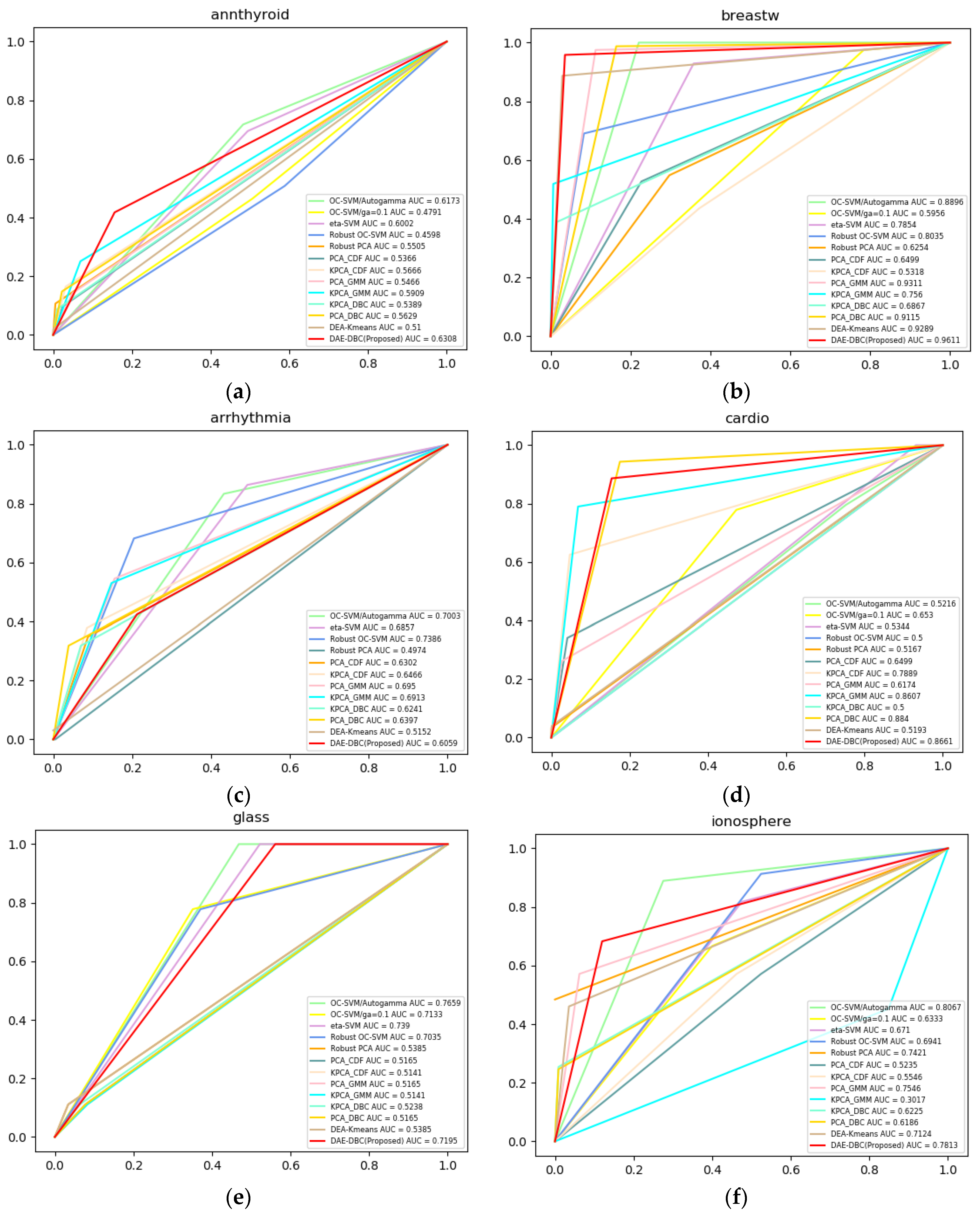
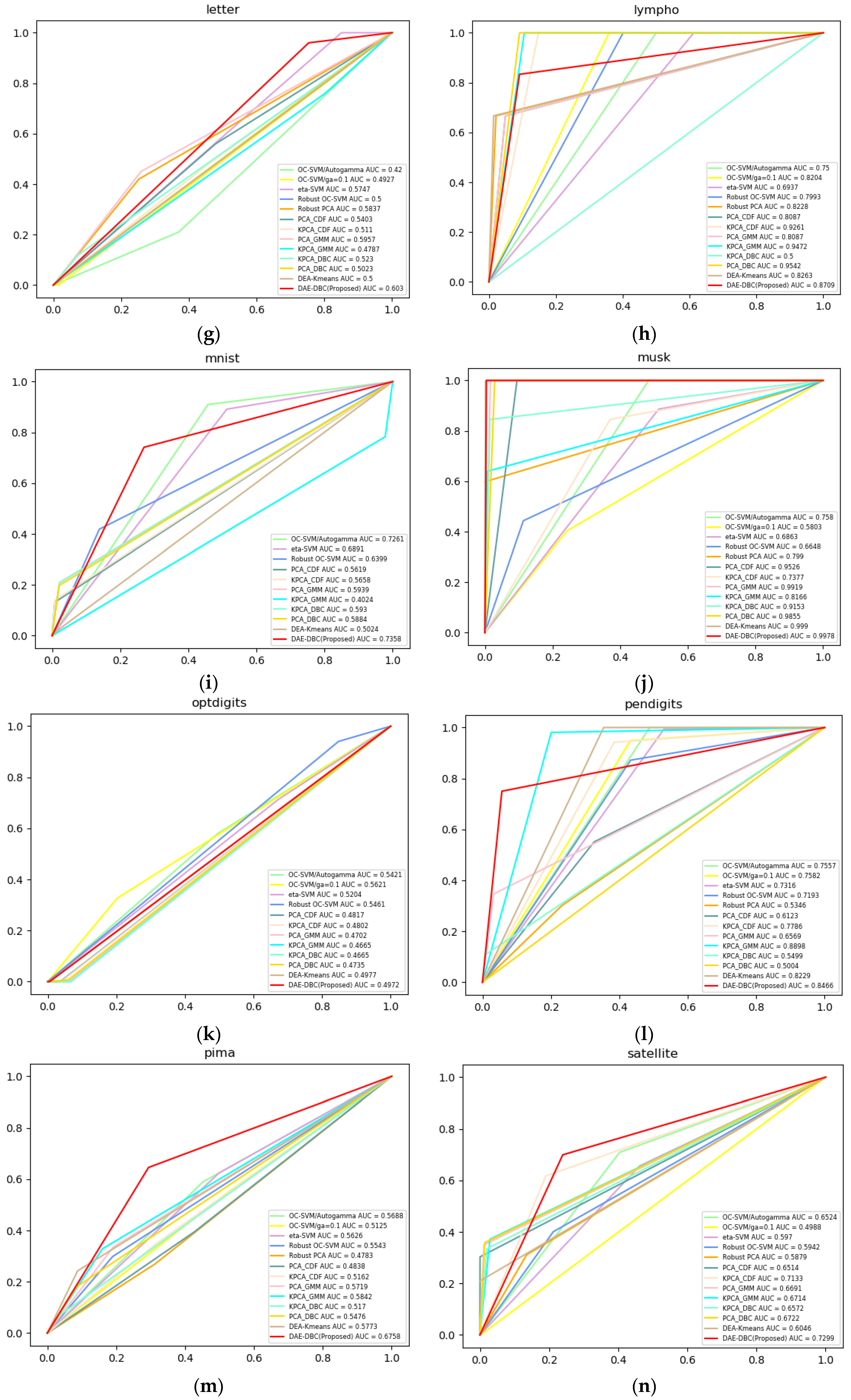
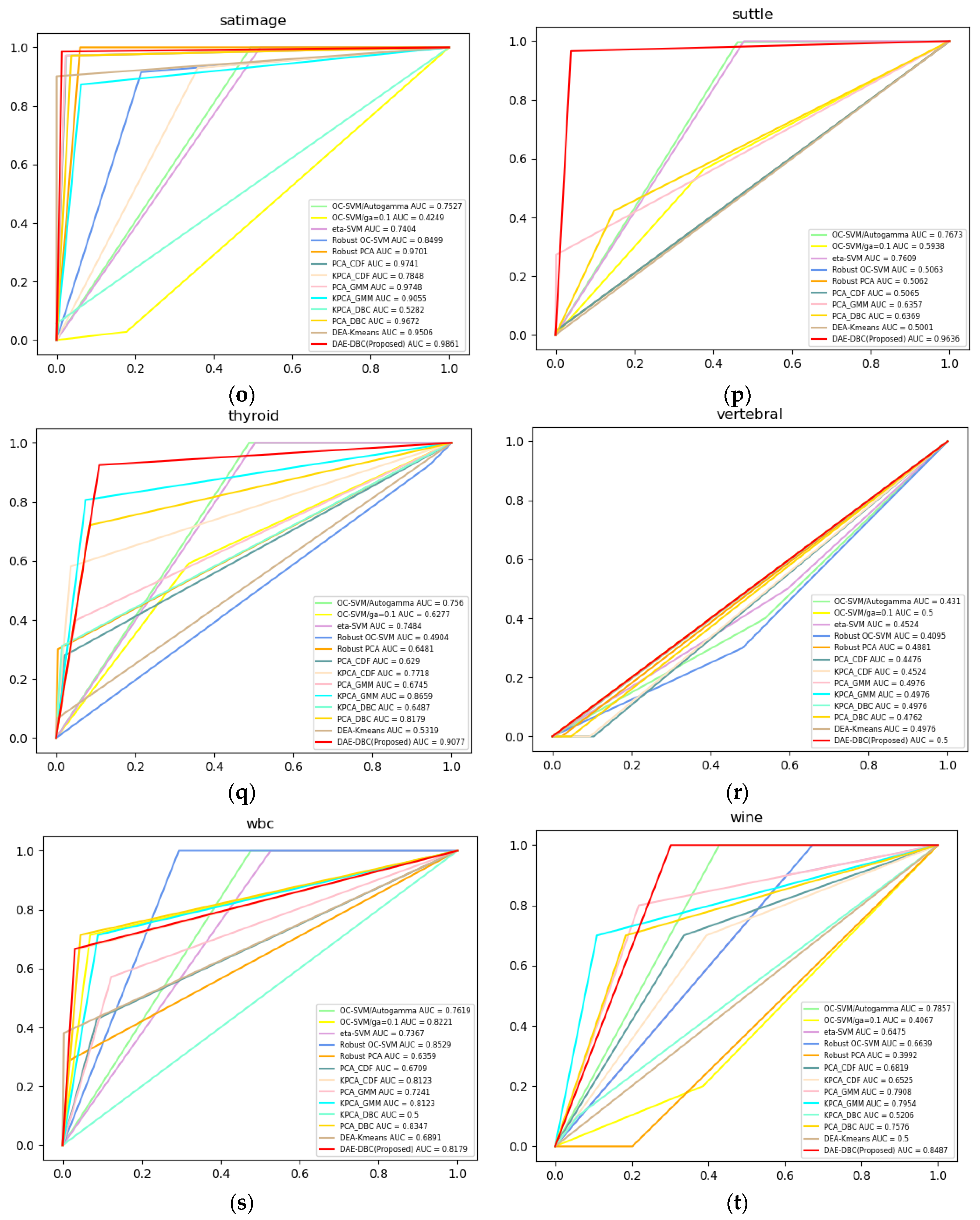
Figure 3 shows the ROC curves of compared 13 methods on 20 different benchmark datasets from ODDS. The DAE-DBC method shows higher AUC scores on 9 of total 20 datasets than other methods. The x-axis is False Positive Rate and the y-axis is True Positive Rate in Figure 3 ROC curves of compared methods.
In order to demonstrate the effectiveness of components together, we have tested multiple variants for replacing components with different algorithms by this experiment. In other words, we used to reduce dimension and get the reconstruction error using AE, then we have made experiments to create PCA-DBC, KPCA-DBC version replacing AE by PCA technique and create DAE-Kmeans version replacing density-based clustering with the K-means algorithm. The DAE-DBC algorithm works better than its other versions and the-state-of-the-art methods that are proposed for other researches.
5. Conclusions
By this paper, we have proposed DAE-DBC approach to detect novelty on unsupervised mode by combining deep autoencoder for low dimensional representation and clustering techniques for novelty estimation. This approach can classify unlabeled dataset with different ratio with normal and novelty by calculating optimal parameters for error threshold and clustering algorithm. We have demonstrated that the components in suggested approach in the experiment has given more efficient results together. DAE-DBC algorithm has improved average AUC of 9 state-of-the-art algorithms on 20 public benchmark datasets by 13.5 percent. Therefore, we suggest this approach on high dimensional data to make unsupervised novelty detection.
Author Contributions
T.A. and B.J. conceived and designed the experiments; T.A. performed the experiments; T.A. and B.J. analyzed the data; T.A and B.J. wrote the paper; K.H.R. supervised, checked, gave comments and approved this work.
Funding
This research was supported by Basic Science Research Program through the National Research Foundation of Korea (NRF) funded by the Ministry of Science, ICT & Future Planning (No. 2017R1A2B4010826).
Conflicts of Interest
The authors declare no conflict of interest.
References
- Chandola, V.; Banerjee, A.; Kumar, V. Anomaly Detection: A Survey. ACM Comput. Surv. 2009, 41, 1–58. [Google Scholar] [CrossRef]
- Tan, P.N.; Steinbach, M.; Kumar, V. Anomaly Detection. In Introduction to Data Mining; Goldstein, M., Harutunian, K., Smith, K., Eds.; Pearson Education Inc.: Boston, MA, USA, 2006; pp. 651–680. ISBN 0-321-32136-7. [Google Scholar]
- Chalapathy, R.; Menon, A.K.; Chawla, S. Anomaly Detection using One-Class Neural Networks. arXiv, 2018; arXiv:1802.06360. [Google Scholar]
- Pascoal, C.; Oliveira, M.R.; Valadas, R.; Filzmoser, P.; Salvador, P.; Pacheco, A. Robust Feature Selection and Robust PCA for Internet Traffic Anomaly Detection. In Proceedings of the IEEE INFOCOM, Orlando, FL, USA, 25–30 March 2012. [Google Scholar]
- Kim, D.P.; Yi, G.M.; Lee, D.G.; Ryu, K.H. Time-Variant Outlier Detection Method on Geosensor Networks. In Proceedings of the International Symposium on Remote Sensing, Daejeon, Korea, 29–31 October 2008. [Google Scholar]
- Lyon, A.; Minchole, A.; Martınez, J.P.; Laguna, P.; Rodriguez, B. Computational techniques for ECG analysis and interpretation in light of their contribution to medical advances. J. R. Soc. Interface 2018, 15. [Google Scholar] [CrossRef] [PubMed]
- Anandakrishnan, A.; Kumar, S.; Statnikov, A.; Faruquie, T.; Xu, D. Anomaly Detection in Finance: Editors’ Introduction. In Proceedings of the Machine Learning Research, Halifax, Nova Scotia, 14 August 2017. [Google Scholar]
- Jin, C.H.; Park, H.W.; Wang, L.; Pok, G.; Ryu, K.H. Short-term Traffic Flow Forecasting using Unsupervised and Supervised Learning Techniques. In Proceedings of the 6th International Conference FITAT and 3rd International Symposium ISPM, Cheongju, Korea, 25–27 September 2013. [Google Scholar]
- Hauskrecht, M.; Batal, I.; Valko, M.; Visweswaran, S.; Cooper, C.F.; Clermont, G. Outlier detection for patient monitoring and alerting. J. Biomed. Inform. 2013, 46, 47–55. [Google Scholar] [CrossRef] [PubMed]
- Cho, Y.S.; Moon, S.C.; Ryu, K.S.; Ryu, K.H. A Study on Clinical and Healthcare Recommending Service based on Cardiovascula Disease Pattern Analysis. Int. J. Biosci. Biotechnol. 2016, 8, 287–294. [Google Scholar] [CrossRef]
- Chawla, N.V.; Japkowicz, N.; Kotcz, A. Editorial: Special Issue on Learning from Imbalanced Data Sets. SIGKDD Explor. Newsl. 2004, 6, 1–6. [Google Scholar] [CrossRef]
- Sarah, M.E.; Rajasegarar, S.; Karunasekera, S.; Leckie, C. High-dimensional and large-scale anomaly detection using a linear one-class SVM with deep learning. Pattern Recognit. 2016, 58, 121–134. [Google Scholar]
- Zimek, A.; Schubert, E.; Kriegel, H.P. A survey on unsupervised outlier detection in high-dimensional numerical data. Stat. Anal. Data Min. 2012, 5, 363–387. [Google Scholar] [CrossRef]
- Rousseeuw, P.J.; Hubert, M. Anomaly Detection by Robust Statistics. WIREs Data Min. Knowl Discov. 2018, 8, 1–30. [Google Scholar] [CrossRef]
- Hoffmann, H. Kernel PCA for novelty detection. Pattern Recognit. 2007, 40, 863–874. [Google Scholar] [CrossRef]
- Zong, B.; Song, Q.; Min, M.R.; Cheng, W.; Lumezanu, C.; Cho, D.; Chen, H. Deep autoencoding gaussian mixture model for unsupervised anomaly detection. In Proceedings of the 6th International Conference on Learning Representations, Vancouver, BC, Canada, 30 April–3 May 2018. [Google Scholar]
- Protopapadakis, E.; Voulodimos, A.; Doulamis, A.; Doulamis, N.; Dres, D.; Bimpas, M. Stacked Autoencoders for Outlier Detection in Over-the-Horizon Radar Signals. Comput. Intell. Neurosci. 2017, 2017. [Google Scholar] [CrossRef] [PubMed]
- Kim, H.; Hirose, A. Unsupervised Fine Land Classification Using Quaternion Autoencoder-Based Polarization Feature Extraction and Self-Organizing Mapping. IEEE Trans. Geosci. Remote Sens. 2018, 56, 1839–1851. [Google Scholar] [CrossRef]
- Elbatta, M.T.; Ashour, W.M. A Dynamic Method for Discovering Density Varied Clusters. International Journal of Signal Processing. Image Process. Pattern Recognit. 2013, 6, 123–134. [Google Scholar]
- Amer, M.; Goldstein, M.; Abdennadher, S. Enhancing One-class Support Vector Machines for Unsupervised Anomaly Detection. In Proceedings of the ACM SIGKDD Workshop on Outlier Detection and Description, Chicago, IL, USA, 11 August 2013. [Google Scholar]
- Ghafoori, Z.; Erfani, S.M.; Rajasegarar, S.; Bezdek, J.C.; Karunasekera, S.; Leckie, C. Efficient Unsupervised Parameter Estimation for One-Class Support Vector Machines. IEEE Trans. Neural Netw. Learn. Syst. 2018, 1–14. [Google Scholar] [CrossRef] [PubMed]
- Yin, S.; Zhu, X.; Jing, C. Fault Detection Based on a Robust One Class Support Vector Machine. Neurocomputing 2014, 145, 263–268. [Google Scholar] [CrossRef]
- Schölkopf, B.; Williamson, R.; Smola, A.; Shawe-Taylor, J.; Platt, J. Support Vector Method for Novelty Detection. In Proceedings of the 12th International Conference on Neural Information Processing Systems, Cambridge, MA, USA, 29 November–4 December 1999. [Google Scholar]
- Zaki, M.J.; Wagner, M., Jr. Data Mining and Analysis: Fundamental Concepts and Algorithms; Cambridge University Press: New York, NY, USA, 2014; ISBN 978-0-521-76633-3. [Google Scholar]
- Kwitt, R.; Hofmann, U. Robust Methods for Unsupervised PCA-based Anomaly Detection. In Proceedings of the IEEE/IST Workshop on “Monitoring, Attack Detection and Mitigation”, Tuebingen, Germany, 28–29 September 2006. [Google Scholar]
- Zhang, Y.D.; Zhang, Y.; Hou, X.X.; Chen, H.; Wang, S.H. Seven-Layer Deep Neural Network Based on Sparse Autoencoder for Voxelwise Detection of Cerebral Microbleed. Multimedia Tools Appl. 2018, 77, 10521–10538. [Google Scholar] [CrossRef]
- Jia, W.; Muhammad, K.; Wang, S.H.; Zhang, Y.D. Five-Category Classification of Pathological Brain Images Based on Deep Stacked Sparse Autoencoder. Multimedia Tools Appl. 2017, 77, 1–20. [Google Scholar] [CrossRef]
- Liou, C.; Cheng, W.; Liou, J.; Liou, D. Autoencoder for Words. Neurocomputing 2014, 139, 84–96. [Google Scholar] [CrossRef]
- Guo, Y.; Liu, Y.; Oerlemans, A.; Lao, S.; Wu, S.; Lew, M.S. Deep Learning for Visual Understanding: A review. Neurocomputing 2016, 187, 27–48. [Google Scholar] [CrossRef]
- Otsu, N. A Threshold Selection Method from Gray-Level Histograms. IEEE Trans. Syst. Man Cybern. 1979, 9, 62–66. [Google Scholar] [CrossRef]
- Ester, M.; Kriegel, H.P.; Sander, J.; Xu, X. A Density-Based Algorithm for Discovering Clusters in Large Spatial Databases with Noise. KDD-96 Proc. 1996, 96, 226–231. [Google Scholar]
- Hodge, V.; Austin, J. A Survey of Outlier Detection Methodologies. Artif. Intell. Rev. 2004, 22, 85–126. [Google Scholar] [CrossRef] [Green Version]
- Bellman, R.E. Adaptive Control Processes: A Guided Tour; Princeton University Press: Princeton, NJ, USA, 1961; ISBN 9781400874668. [Google Scholar]
- Rayana, S. ODDS. Stony Brook University, Department of Computer Sciences, 2016. Available online: http://odds.cs.stonybrook.edu/ (accessed on 30 July 2018).
- Yu, J. Fault Detection Using Principal Components-Based Gaussian Mixture Model for Semiconductor Manufacturing Processes. IEEE Trans. Semicond. Manuf. 2011, 24, 432–444. [Google Scholar] [CrossRef]
- Kim, J.; Grauman, K. Observe locally, infer globally: A space-time MRF for detecting abnormal activities with incremental updates. In Proceedings of the IEEE Conference on Computer Vision and Pattern Recognition, Miami, FL, USA, 20–25 June 2009. [Google Scholar]
- Rousseeuw, P.J. Silhouettes: A Graphical Aid to the Interpretation and Validation of Cluster Analysis. J. Comput. Appl. Math. 1987, 20, 53–65. [Google Scholar] [CrossRef]
- Kingma, D.P.; Ba, J. Adam: A method for stochastic optimization. In Proceedings of the 3rd International Conference for Learning Representations, San Diego, CA, USA, 7–9 May 2014. [Google Scholar]
Figure 1.
General architecture of proposed method.

Figure 2.
Deep autoencoder model.

Figure 3.
ROC curves of compared methods. (a) Annthyroid, 6 dimension, novelty ratio 0.08; (b) BreastW, 9 dimension, novelty ratio 0.53; (c) Arrhythmia, 274 dimension, novelty ratio 0.17; (d) Cardio, 21 dimension, novelty ratio 0.1; (e) Glass, 9 dimension, novelty ratio 0.04; (f) Ionosphere, 33 dimension, novelty ratio 0.56; (g) Letter, 32 dimension, novelty ratio 0.06; (h) Lympho, 18 dimension, novelty ratio; (i) Mnist, 100 dimension, novelty ratio 0.1; (j) Musk, 72 dimension, novelty ratio; (k) Optdigits, 64 dimension, novelty ratio 0.03; (l) Pendigits, 16 dimension, novelty ratio 0.02; (m) Pima, 8 dimension, novelty ratio 0.5; (n) Satellite, 36 dimension, novelty ratio 0.46; (o) Satimage, 36 dimension, novelty ratio 0.01; (p) Suttle, 9 dimension, novelty ratio 0.07; (q) Thyroid, 6 dimension, novelty ratio 0.02; (r)Vertebral, 6 dimension, novelty ratio 0.14; (s) Wbc, 30 dimension, novelty ratio 0.05; (t) Wine, 13 dimension, novelty ratio 0.08.


Table 1.
Description of datasets.
| Dataset | Dim | Instance | Normal | Novelty | Description |
|---|---|---|---|---|---|
| BreastW | 10 | 683 | 444 | 239 | There are two classes, benign and malignant. The malignant class is considered as novelty. |
| Annthyroid | 6 | 7200 | 6666 | 534 | There are three classes are built: normal, hyperfunction and subnormal functioning. The hyperfunction and subnormal classes are treated as novelty class. |
| Arrhythmia | 274 | 452 | 386 | 66 | It is a multi-class classification dataset. The smallest classes, i.e., 3, 4, 5, 7, 8, 9, 14, 15 are combined to form the novelty class. |
| Cardio | 21 | 1831 | 1655 | 176 | There are 3 classes, normal, suspect and pathologic. Pathologic (novelty) class is downsampled to 176 points. The suspect class is discarded. |
| Glass | 9 | 214 | 205 | 9 | This dataset contains attributes regarding several glass types (multi-class). Here, class 6 is marked as novelty. |
| Ionosphere | 33 | 351 | 225 | 126 | There is one attribute having values all zeros, which is discarded. So, the total number of dimensions are 33. The ‘bad’ class is considered as novelty class. |
| Letter | 32 | 1600 | 1500 | 100 | 3 letters from data was sampled to form the normal class and randomly concatenate pairs of them to form the novelty class. |
| Lympho | 18 | 148 | 142 | 6 | It has four classes but two of them are quite small. Therefore, those two small classes are merged and considered as novelty. |
| Mnist | 100 | 7603 | 6903 | 700 | Digit-zero class is considered as inliers, while 700 images are sampled from digit-six class as the outliers. |
| Musk | 72 | 3062 | 2965 | 97 | The non-musk classes, j146, j147 and 252 are combined to form the inliers, while the musk classes 213 and 211 are added as novelty without downsampling. Other classes are discarded. |
| Optdigits | 64 | 5216 | 5066 | 150 | The instances of digits 1-9 are inliers and instances of digit 0 are down-sampled to 150 outliers. |
| Pendigits | 16 | 6870 | 6714 | 156 | It has10 classes (0 … 9). In this dataset, all classes have equal frequencies. So, the number of objects in one class (corresponding to the digit “0”) is reduced by a factor of 10%. |
| Pima | 8 | 768 | 500 | 268 | Several constraints were placed on the selection of instances from a larger database. In particular, all patients here are females at least 21 years old of Pima Indian heritage. |
| Satellite | 36 | 6435 | 4399 | 2036 | The smallest three classes, i.e., 2, 4, 5 are combined to form the outliers’ novelty. |
| Satimage | 36 | 5803 | 5732 | 71 | Class 2 is down-sampled to 71 outliers, while all the other classes are combined to form an inlier class. |
| Suttle | 9 | 49097 | 45586 | 3511 | The smallest 5 classes, i.e., 2, 3, 5, 6, 7 are combined to form the novelty class, while class 1 forms the inlier class. Data for class 4 is discarded. |
| Thyroid | 6 | 3772 | 3679 | 93 | There are 3 classes are built: normal, hyperfunction and subnormal functioning. The hyperfunction class is treated as novelty class. |
| Vertebral | 6 | 240 | 210 | 30 | The following convention is used for the class labels: Normal (NO) and Abnormal (AB). Here, “AB” is the majority class having 210 instances which are used as inliers and “NO” is downsampled from 100 to 30 instances as outliers. |
| WBC | 30 | 378 | 357 | 21 | There are 2 classes, benign and malignant. The malignant class of this dataset is downsampled to 21 points, which are considered as novelty. |
| Wine | 13 | 129 | 119 | 10 | Class 1 is downsampled to 10 instances to be used as novelty. |
Table 2.
AUC score comparison between Algorithm 1 and Algorithm 3. The highest values of AUC scores are marked in bold.
Table 2.
AUC score comparison between Algorithm 1 and Algorithm 3. The highest values of AUC scores are marked in bold.
| Dataset | Algorithm 1 | Algorithm 3 |
|---|---|---|
| Annthyroid | 0.5866 | 0.6308 |
| Breastw | 0.8962 | 0.9767 |
| Arrhythmia | 0.9181 | 0.6966 |
| Cardio | 0.7837 | 0.8661 |
| Glass | 0.4580 | 0.7195 |
| Ionosphere | 0.7440 | 0.7813 |
| Letter | 0.5957 | 0.6030 |
| Lympho | 0.7500 | 0.8709 |
| Mnist | 0.7315 | 0.7358 |
| Musk | 0.9266 | 0.9978 |
| Optdigits | 0.6108 | 0.4972 |
| Pendigits | 0.7861 | 0.8466 |
| Pima | 0.6423 | 0.6758 |
| Satellite | 0.6696 | 0.7299 |
| Satimage | 0.9204 | 0.9861 |
| Suttle | 0.9427 | 0.9695 |
| Thyroid | 0.9554 | 0.9077 |
| Vertebral | 0.4000 | 0.5000 |
| Wbc | 0.8221 | 0.8179 |
| Wine | 0.8487 | 0.8487 |
Table 3.
AUC score of compared methods on benchmark datasets. The highest values of AUC scores are marked in bold.
Table 3.
AUC score of compared methods on benchmark datasets. The highest values of AUC scores are marked in bold.
| RapidMiner/Extension of Outlier Detection/ | Python Implementation/Using Keras/ | ||||||||||||
|---|---|---|---|---|---|---|---|---|---|---|---|---|---|
| Dataset | OC-SVM /auto gamma, nu=0.5/ | OC-SVM /gamma=0.1, nu=0.5/ | eta-SVM /auto gamma, nu=0.5/ | Robust-SVM /auto gamma, nu=0.5/ | Robust-PCA | PCA-CDF | KPCA-CDF | PCA-GMM | KPCA-GMM | PCA-DBC | KPCA-DBC | DAE-Kmeans | DAE-DBC (Proposed) |
| Annthyroid | 0.6173 | 0.4791 | 0.6002 | 0.4598 | 0.5505 | 0.5366 | 0.5666 | 0.5466 | 0.5909 | 0.5629 | 0.5389 | 0.5100 | 0.6308 |
| Breastw | 0.8896 | 0.5956 | 0.7854 | 0.8035 | 0.6254 | 0.6499 | 0.5318 | 0.9311 | 0.7560 | 0.9115 | 0.6867 | 0.9289 | 0.9767 |
| Arrhythmia | 0.7003 | NA | 0.6857 | 0.7386 | 0.4974 | 0.6302 | 0.6466 | 0.6950 | 0.6913 | 0.6397 | 0.6241 | 0.5152 | 0.6966 |
| Cardio | 0.5216 | 0.6530 | 0.5344 | 0.5000 | 0.5167 | 0.6499 | 0.7889 | 0.6174 | 0.8607 | 0.8840 | 0.5000 | 0.5193 | 0.8661 |
| Glass | 0.7659 | 0.7133 | 0.7390 | 0.7035 | 0.5385 | 0.5165 | 0.5141 | 0.5165 | 0.5141 | 0.5165 | 0.5238 | 0.5385 | 0.7195 |
| Ionosphere | 0.8067 | 0.6333 | 0.6710 | 0.6941 | 0.7421 | 0.5235 | 0.5546 | 0.7546 | 0.3017 | 0.6186 | 0.6225 | 0.7124 | 0.7813 |
| Letter | 0.4200 | 0.4927 | 0.5747 | 0.5000 | 0.5837 | 0.5403 | 0.7400 | 0.5957 | 0.4787 | 0.5023 | 0.5230 | 0.5000 | 0.6030 |
| Lympho | 0.7500 | 0.8204 | 0.6937 | 0.7993 | 0.8228 | 0.8087 | 0.9261 | 0.8087 | 0.9472 | 0.9542 | 0.5000 | 0.8263 | 0.8709 |
| Mnist | 0.7261 | NA | 0.6891 | 0.6399 | NA | 0.5619 | 0.5658 | 0.5939 | 0.4024 | 0.5884 | 0.5930 | 0.5024 | 0.7358 |
| Musk | 0.7580 | 0.5803 | 0.6863 | 0.6648 | 0.7990 | 0.9526 | 0.7377 | 0.9919 | 0.8166 | 0.9855 | 0.9153 | 0.9990 | 0.9978 |
| Optdigits | 0.5421 | 0.5621 | 0.5204 | 0.5461 | NA | 0.4817 | 0.4980 | 0.4702 | 0.4665 | 0.4735 | 0.4665 | 0.8229 | 0.4972 |
| Pendigits | 0.7557 | 0.7582 | 0.7316 | 0.7193 | 0.5346 | 0.6123 | 0.7786 | 0.6569 | 0.8898 | 0.5004 | 0.5499 | 0.6926 | 0.8466 |
| Pima | 0.5688 | 0.5125 | 0.5626 | 0.5543 | 0.4783 | 0.4838 | 0.5162 | 0.5719 | 0.5842 | 0.5476 | 0.5170 | 0.5773 | 0.6758 |
| Satellite | 0.6524 | 0.4988 | 0.5970 | 0.5942 | 0.5879 | 0.6514 | 0.7133 | 0.6691 | 0.6714 | 0.6722 | 0.6572 | 0.6046 | 0.7299 |
| Satimage | 0.7527 | 0.4249 | 0.7404 | 0.8499 | 0.9701 | 0.9741 | 0.7848 | 0.9748 | 0.9055 | 0.9672 | 0.5282 | 0.9506 | 0.9861 |
| Suttle | 0.7673 | 0.5938 | 0.7609 | 0.5063 | 0.5062 | 0.5065 | NA | 0.6357 | NA | 0.6369 | NA | 0.5001 | 0.9695 |
| Thyroid | 0.7560 | 0.6277 | 0.7484 | 0.4904 | 0.6481 | 0.6290 | 0.7718 | 0.6745 | 0.8659 | 0.8179 | 0.6487 | 0.5319 | 0.9077 |
| Vertebral | 0.4310 | 0.5000 | 0.4524 | 0.4095 | 0.4881 | 0.4476 | 0.4524 | 0.4976 | 0.4976 | 0.4762 | 0.4976 | 0.4976 | 0.5000 |
| Wbc | 0.7619 | 0.8221 | 0.7367 | 0.8529 | 0.6359 | 0.6709 | 0.8123 | 0.7241 | 0.8123 | 0.8347 | 0.5000 | 0.6891 | 0.8179 |
| Wine | 0.7857 | 0.4067 | 0.6475 | 0.6639 | 0.3992 | 0.6819 | 0.6525 | 0.7908 | 0.7954 | 0.7576 | 0.5206 | 0.5000 | 0.8487 |
| Average AUC | 0.6865 | 0.5930 | 0.6579 | 0.6345 | 0.6069 | 0.6255 | 0.6606 | 0.6858 | 0.6762 | 0.6924 | 0.5744 | 0.6459 | 0.7829 |
Table 4.
Comparison of computation time of algorithms.
| RapidMiner/Extension of Outlier Detection/ | Python Implementation/Using Keras/ | ||||||||||||
|---|---|---|---|---|---|---|---|---|---|---|---|---|---|
| Dataset | OC-SVM /auto gamma, nu=0.5/ | OC-SVM /gamma=0.1, nu=0.5/ | eta-SVM /auto gamma, nu=0.5/ | Robust-SVM /auto gamma, nu=0.5/ | Robust-PCA | PCA-CDF | KPCA-CDF | PCA-GMM | KPCA-GMM | PCA-DBC | KPCA-DBC | DAE-Kmeans | DAE-DBC (Proposed) |
| Annthyroid | 40 | 66 | 46 | 46 | 0.11 | 0.25 | 24.662 | 0.467 | 28.491 | 26.576 | 33.581 | 2002.1 | 261.46 |
| Breastw | 44 | 7 | 46 | 6 | 0.153 | 0.463 | 0.477 | 0.492 | 0.666 | 22.22 | 21.874 | 115.32 | 31.764 |
| Arrhythmia | 0< | NA | 1 | 0< | 0.063 | 0.082 | 0.206 | 0.111 | 0.394 | 6.737 | 9.155 | 105.33 | 32.916 |
| Cardio | 12 | 24 | 15 | 16 | 0.107 | 0.227 | 1.564 | 0.326 | 1.824 | 9.027 | 7.735 | 152.27 | 71.649 |
| Glass | 0< | 0< | 0< | 0< | 0.025 | 0.034 | 0.059 | 0.084 | 0.156 | 8.164 | 5.286 | 32.869 | 14.515 |
| Ionosphere | 0< | 0< | 0< | 0< | 0.041 | 0.069 | 0.115 | 0.138 | 0.263 | 32.845 | 5.919 | 39.85 | 19.17 |
| Letter | 5 | 11 | 7 | 7 | 0.072 | 0.267 | 1.349 | 0.315 | 1.574 | 9.577 | 9.775 | 113.1 | 60.347 |
| Lympho | 0< | 0< | 0< | 0< | 0.027 | 0.041 | 0.164 | 0.077 | 0.219 | 3.613 | 7.435 | 22.957 | 15.056 |
| Mnist | 1330 | NA | 1134 | 1111 | NA | 3.378 | 41.538 | 2.789 | 43.302 | 27.391 | 35.814 | 754.57 | 268.66 |
| Musk | 50 | 90 | 71 | 73 | 0.204 | 0.691 | 6.714 | 0.660 | 7.116 | 10.253 | 10.989 | 322.09 | 136.11 |
| Optdigits | 124 | 201 | 142 | 146 | NA | 0.923 | 15.405 | 0.997 | 16.585 | 29.792 | 21.358 | 509.33 | 180.97 |
| Pendigits | 31 | 42 | 31 | 36 | 0.262 | 0.561 | 23.313 | 0.656 | 24.260 | 23.485 | 30.98 | 637.16 | 221.27 |
| Pima | 0< | 0< | 0< | 0< | 0.037 | 0.112 | 0.360 | 0.166 | 0.497 | 7.867 | 5.266 | 80.555 | 28.045 |
| Satellite | 66 | 96 | 71 | 78 | 0.207 | 0.685 | 21.680 | 0.798 | 24.556 | 22.789 | 58.857 | 686.85 | 236.33 |
| Satimage | 42 | 58 | 44 | 55 | 0.187 | 0.642 | 17.275 | 0.849 | 18.386 | 2.419 | 21.31 | 592.40 | 217.29 |
| Suttle | 19,908 | 19,761 | 22,431 | 22,891 | 0.577 | 1.437 | NA | 1.780 | NA | 139.98 | NA | 5419.4 | 1753.7 |
| Thyroid | 13 | 18 | 15 | 17 | 0.088 | 0.207 | 5.677 | 0.271 | 6.097 | 13.092 | 17.961 | 328.83 | 218.54 |
| Vertebral | 0< | 0< | 0< | 0< | 0.07 | 0.060 | 0.060 | 0.107 | 0.111 | 4.497 | 9.151 | 37.441 | 20.874 |
| Wbc | 0< | 0< | 0< | 0< | 0.05 | 0.148 | 0.166 | 0.169 | 0.212 | 4.043 | 3.269 | 72.288 | 46.738 |
| Wine | 0< | 0< | 0< | 0< | 0.028 | 0.055 | 0.044 | 0.083 | 0.098 | 3.929 | 8.441 | 20.71 | 26.951 |
© 2018 by the authors. Licensee MDPI, Basel, Switzerland. This article is an open access article distributed under the terms and conditions of the Creative Commons Attribution (CC BY) license (http://creativecommons.org/licenses/by/4.0/).
Share and Cite
MDPI and ACS Style
Amarbayasgalan, T.; Jargalsaikhan, B.; Ryu, K.H. Unsupervised Novelty Detection Using Deep Autoencoders with Density Based Clustering. Appl. Sci. 2018, 8, 1468. https://doi.org/10.3390/app8091468
AMA Style
Amarbayasgalan T, Jargalsaikhan B, Ryu KH. Unsupervised Novelty Detection Using Deep Autoencoders with Density Based Clustering. Applied Sciences. 2018; 8(9):1468. https://doi.org/10.3390/app8091468
Chicago/Turabian StyleAmarbayasgalan, Tsatsral, Bilguun Jargalsaikhan, and Keun Ho Ryu. 2018. "Unsupervised Novelty Detection Using Deep Autoencoders with Density Based Clustering" Applied Sciences 8, no. 9: 1468. https://doi.org/10.3390/app8091468
Note that from the first issue of 2016, this journal uses article numbers instead of page numbers. See further details here.