SD-EAR: Energy Aware Routing in Software Defined Wireless Sensor Networks

1
Department of Computer Applications, Kalyani Government Engineering College, Nadia 741325, West Bengal, India
2
Department of Energy Technology, Aalborg University, 9100 Esbjerg, Denmark
*
Author to whom correspondence should be addressed.
Appl. Sci. 2018, 8(7), 1013; https://doi.org/10.3390/app8071013
Submission received: 10 May 2018
/
Revised: 25 May 2018
/
Accepted: 29 May 2018
/
Published: 21 June 2018
Abstract
:In today’s internet-of-things (IoT) environment, wireless sensor networks (WSNs) have many advantages, with broad applications in different areas including environmental monitoring, maintaining security, etc. However, high energy depletion may lead to node failures in WSNs. In most WSNs, nodes deplete energy mainly because of the flooding and broadcasting of route-request (RREQ) packets, which is essential for route discovery in WSNs. The present article models wireless sensor networks as software-defined wireless sensor networks (SD-WSNs) where the network is divided into multiple clusters or zones, and each zone is controlled by a software-defined network (SDN) controller. The SDN controller is aware of the topology of each zone, and finds out the optimum energy efficient path from any source to any destination inside the zone. For destinations outside of the zone, the SDN controller of the source zone instructs the source to send a message to all of the peripheral nodes in that zone, so that they can forward the message to the peripheral nodes in other zones, and the process goes on until a destination is found. As far as energy-efficient path selection is concerned, the SDN controller of a zone is aware of the connectivity and residual energy of each node. Therefore, it is capable of discovering an optimum energy efficient path from any source to any destination inside as well as outside of the zone of the source. Accordingly, flow tables in different routers are updated dynamically. The task of route discovery is shifted from individual nodes to controllers, and as a result, the flooding of route-requests is completely eliminated. Software-defined energy aware routing (SD-EAR)also proposes an innovative sleeping strategy where exhausted nodes are allowed to go to sleep through a sleep request—sleep grant mechanism. All of these result in huge energy savings in SD-WSN, as shown in the simulation results.
1. Introduction
The internet of things (IoT) has gained considerable attention recently from industry and academia. An important component of IoT is wireless sensor networks (WSN). Energy efficiency in the routing of WSNs is extremely necessary to preserve energy and increase the lifetime of nodes [1,2,3,4,5,6,7,8,9,10,11,12,13,14,15,16,17,18,19,20,21,22,23,24,25,26,27,28,29,30,31,32,33,34,35,36,37,38,39,40,41,42,43]. Nodes in wireless sensor networks deplete quickly if a huge number of route discoveries are initiated. One route discovery means the broadcasting of route-request to all of the nodes in the network. This requires an excessive number of unnecessary forwarding of route-requests, especially if the source or the routers do not know of a recent destination or location. In order to save energy, nodes try to go to sleep, but there is no central authority who can judge whether the sleep request is valid or not. Therefore, nodes take decisions on their own, and this information is propagated only to its neighbors; it cannot be circulated throughout the network to avoid energy consumption. Therefore, if a source wants to communicate with one such sleeping node, then all of its associated forwarding of route-requests will go in vain.
1.1. What is SDN?
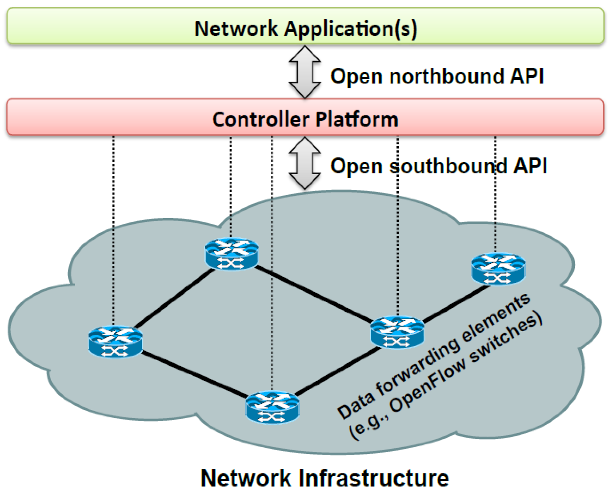
Software defined networking (SDN) is a recent trend of a network that introduces the idea of eliminating tight coupling between the control and the forwarding plane. The network can be broadly divided into three components: a centralized controller, hosts, and switches that connect a pair of hosts, a pair of switches, or a host–switch pair. Northbound and southbound application programming interfaces (APIs) are there to establish communication between various network entities. The centralized controller has the responsibility of configuring forwarding planes (popularly termed as flow tables) according to which switches forward the packets during communication. The basic structure of an SDN appears in Figure 1.
SDN is deployed in various types of networks, such as LAN, MAN, WAN, data center networks, etc. The advantages are flexible network control without sacrificing forwarding performance, ease of implementation, administration, and ample opportunities of reducing energy consumption [44,45]. SDN has proven to be extremely successful in highly scalable data centers extending from private enterprises to public sectors where managing big data is not the only issue [8,9,10]; thousands of new data are being generated every day to satisfy the requirements of various applications initiated by different levels of users. OpenFlow-based SDN data centers have set a new trend as far as performance efficiency is concerned. Scheduling the flows to various ports is a very important component of network flow control. Also, the occasional deactivation of switches is required to preserve energy.
Reduction of energy consumption is an important aspect of efficiency in SDN.
1.2. Contributions of the Present Paper
In the present paper, software defined energy aware routing (SD-EAR) and SDN divide the completely distributed structure of a sensor network into clusters or zones where each controller is in charge of one zone. The controllers are aware of the topologies of the associated zone, and also keep track of peripheral nodes. Peripheral nodes in a zone are nodes that have some portion of radio circle outside the zone. SD-EAR particularly aims at proposing an energy-efficient routing protocol along with a sleeping strategy to promote energy preservation in the network. Its novelties are as follows:
- (i)
- Normally in a WSN, whenever a source needs to establish a route to a sink, it mostly applies blind flooding [27,33,38,39] or gossiping [38,39]. In flooding, each router retransmits the route-request (RREQ) generated by a source to all of its neighbors, whereas the gossiping technique enables the routers to select a subset of neighbors to rebroadcast the route-request packet. Both of these suffer from redundancies that unnecessarily eat up energies in routers. In SD-EAR, since the SDN controller of each zone is aware of the zonal topology, it is capable of finding all of the possible paths between a given source and a destination through the depth-first traversal technique if both the source and destination are within the same zone. Among all of these paths, one optimal path is selected by a fuzzy controller named FUZZ-OPT-ROUTE, which is embedded within each SDN controller. If the destination is not within same zone as the source, then the SDN controller of the source zone instructs the source to send a request for discovering the route to the destination or to all of the peripheral nodes in the zone, through the optimum paths selected by the FUZZ-OPT-ROUTE embedded in the SDN controller of the source. Routers perform similar to the source. SD-EAR gives special weight to the presence of alternative nodes in live communication paths. As a result, the broadcasting of a route-request is eliminated irrespective of intra-zone or inter-zone communication, resulting in huge message saving.
- (ii)
- An alternative node nv of a node nu in a live communication route R, should be such that energy efficiency as well as the lifetime of R should not decrease after replacing nu with nv. This provides a facility to improve the residual energy and lifetime of a route. It may happen that after replacing the least energy node with an alternative, the new minimum energy becomes higher than the previous minimum. In that case, the new minimum will depend upon other nodes in the route except the one with the previous minimum energy. Assuming all of these nodes to be equally likely, we consider both the minimum and average residual energy to compute the residual energy effect of a route. Please note that the alternatives for a node are searched if its battery is almost exhausted.
- (iii)
- A sleeping strategy is also proposed where nodes that request to go to sleep are granted sleep by the SDN controller of the zone, provided the situation demands so. All of these help to greatly reduce the energy consumption in the network, and increase network throughput. Also, the provision of forceful sleep is introduced in which if all of the neighbors of a node are suffering from exhausted battery, then nu is directed by the SDN controller to go to sleep. All of these result in great energy saving by avoiding the broadcasting of route-requests during route discovery as well as rediscovery.
1.3. Organization of the Article
2. Related Work
Currently, most applications and services in WSN, such as network flexibility, network management, energy conservation, network robustness, and packet loss probability, rely on a data exchange between the sensor nodes and the switch infrastructure, or among sensor nodes. We divide all of the energy-efficient approaches to WSNs in two groups: non-software defined and software defined. These are described below.
2.1. Non-Software Defined Energy-Efficient Approaches
LEACH (Low energy adaptive clustering hierarchy), SPIN (Sensor protocol for information via negotiation), threshold-sensitive energy-efficient sensor networks (TEEN), etc. are extremely important from the perspective of non-software defined energy efficiency in sensor networks. The idea of LEACH protocol is to organize the sensor nodes into clusters, where each cluster has one cluster head CH that acts as a router to the base station. However, the LEACH protocol has problems; one of those problems is the random selection of a cluster head or CHs [35,36,43]. This process does not consider the location of sensor nodes in the wireless sensor network, and hence, the sensor nodes may be very far from their CH, causing them to consume more energy to communicate with the CH [35,36,43]. The role of the cluster head is rotated in order to balance the energy consumption among multiple nodes. The optimum route chosen for communication is the shortest one computed using Dijkstra’s shortest path algorithm [36]. However, the shortest route is not always the most energy-efficient option.
SPIN [38] is another energy-efficient routing protocol worthy of mention; which is a modification of classic flooding. In classical flooding, the information is forwarded on every outgoing link of a node. This drains out the battery of a huge number of nodes in the sensor network. SPIN was developed to overcome this drawback. It is an adaptive routing protocol that transmits the information first by negotiating. It proposes the use of metadata of actual data to be sent. Metadata contains a description of the actual message that the node wants to send. Actual data will be transmitted only if the node wishes to receive it, that is, it is similar to being keen to watch a movie after viewing its trailer. In this context, we humbly state that SPIN requires the broadcasting of metadata at least. However, an important aspect of the energy efficiency of SD-EAR arises from it not requiring broadcasting to establish routes.
TEEN (threshold-sensitive energy-efficient sensor networks) [46] protocol was proposed for time-critical applications. Here, sensor nodes sense the medium continuously, but data transmission is done less frequently. A cluster head sensor sends its members a hard threshold (HT), which is the threshold value of sensed attribute, and a soft threshold (ST), which is a small change in the value of the sensed attribute that triggers the node to switch on its transmitter and transmit. The main drawback of this scheme is that if the thresholds are not received, the nodes will never communicate, and the user will not get any data from the network at all. Also, it has the complexity associated with forming clusters at multiple levels and the method of implementing threshold-based functions [46].
2.2. Software Defined Energy-Efficient Approaches
Figueiredo et al. [12] used multiple adaptive hybrid approaches, which are considered better than a single algorithm. This work (which subsequently will be referred to as software defined wireless sensor network 1, or SD-WSN1, in this article) discusses the usage of policies to establish adaptive routing rules so that the WSN elements of a network can acquire more flexible and accessible development and maintenance tasks. The routing policy is either proactive or reactive. If the number of nodes in the network is less than a pre-defined threshold, then proactive routing is applied to determine the forwarding rules in order to save the cost of route discovery. However, if the number of nodes in the network crosses a pre-defined threshold, then proactive routing becomes impossible due to an abnormal rise in the size of the flow table. Reactive routing follows the behavior of ad hoc distance vector routing, or AODV. This applies flooding for route discovery. Ejaz et al. [20] designed an energy-efficient SD-WSN (which subsequently will be referred to as SD-WSN2 in this article) to minimize the energy consumption of energy transmitters. This article is based on the energy that is transferred to sensor nodes through energy transmitters. It aims at the optimal placement of energy transmitters, which depends on the trade-off between the minimum energy charged in the network and a fair distribution of energy. This does not propose any energy-efficient routing protocol or sleeping strategy of nodes. Xiang et al. [21] studied an energy-efficient routing algorithm for SD-WSN (which subsequently will be referred to as SD-WSN3 in this article) by selecting the control nodes and assigning different tasks dynamically through control nodes. SD-WSN3 selects some control nodes out of all of the nodes in the network using the particle swarm optimization method. These nodes assign tasks to others depending upon their residual energy. However, it is very difficult to determine the exact number of required control nodes, and how many nodes will be under the control of one particular control node.
Luo et al. [10] proposed a software-defined WSN architecture to solve the rigidity of policies and the difficulty of management by addressing Sensor OpenFlow. Jacobsson and Orfanidis [11] adopted low-cost off-the-shelf hardware and an individual deployment method to flexibly reconfigure WSN networking and in-network processing functionality. Regarding the network management, Gante et al. [13] presented a smart management in WSN by employing the OpenFlow protocol and modifying the forwarding rule in the controller, which can use the unified standard to communicate with all of the nodes. A networking solution called SDN-WISE was proposed by Galluccio et al. [14] to simplify the management of the network. Olivier et al. [15] proposed a cluster-based architecture with multiple base stations used as hosts for the SDN control functions as well as cluster heads, and adopted a structured and hierarchical management. Modieginyane et al. [16] summarized the application challenges faced by WSNs for monitored environments and the opportunities that can be realized in applications of WSNs using SDN.
Jayashree et al. [19] proposed a framework for a software-defined wireless sensor network, where the sensor node only performed the forwarding. The controller was implemented as the base station in this framework, thus reducing the energy consumption. For packet loss probability and robustness, Levendovszky et al. [22] provided the Hopfield neural network to guarantee uniform packet loss probabilities for the nodes. Sachenko et al. [23] presented modified correction codes based on a residual number system, high correction characteristics, and a simplified coding procedure to show the characteristics of these codes, which can improve the data transmission robustness in WSN.
Jin et al. [24] dealt with the packet loss by designing a hierarchical data transmission framework of a suitable industrial environment. For a real industrial environment, the commonly-used WSN framework discussed above is not well suited to the environment’s unique characteristics, such as a harsh application environment, a strict requirement for data transmission, data diversity, and so on. The traditional SD-WSN framework is a universal network framework that is not specific to the IoT. In order to resolve these problems and adapt the framework for an industrial environment, we will present an improved SD-WSN framework in the next section.
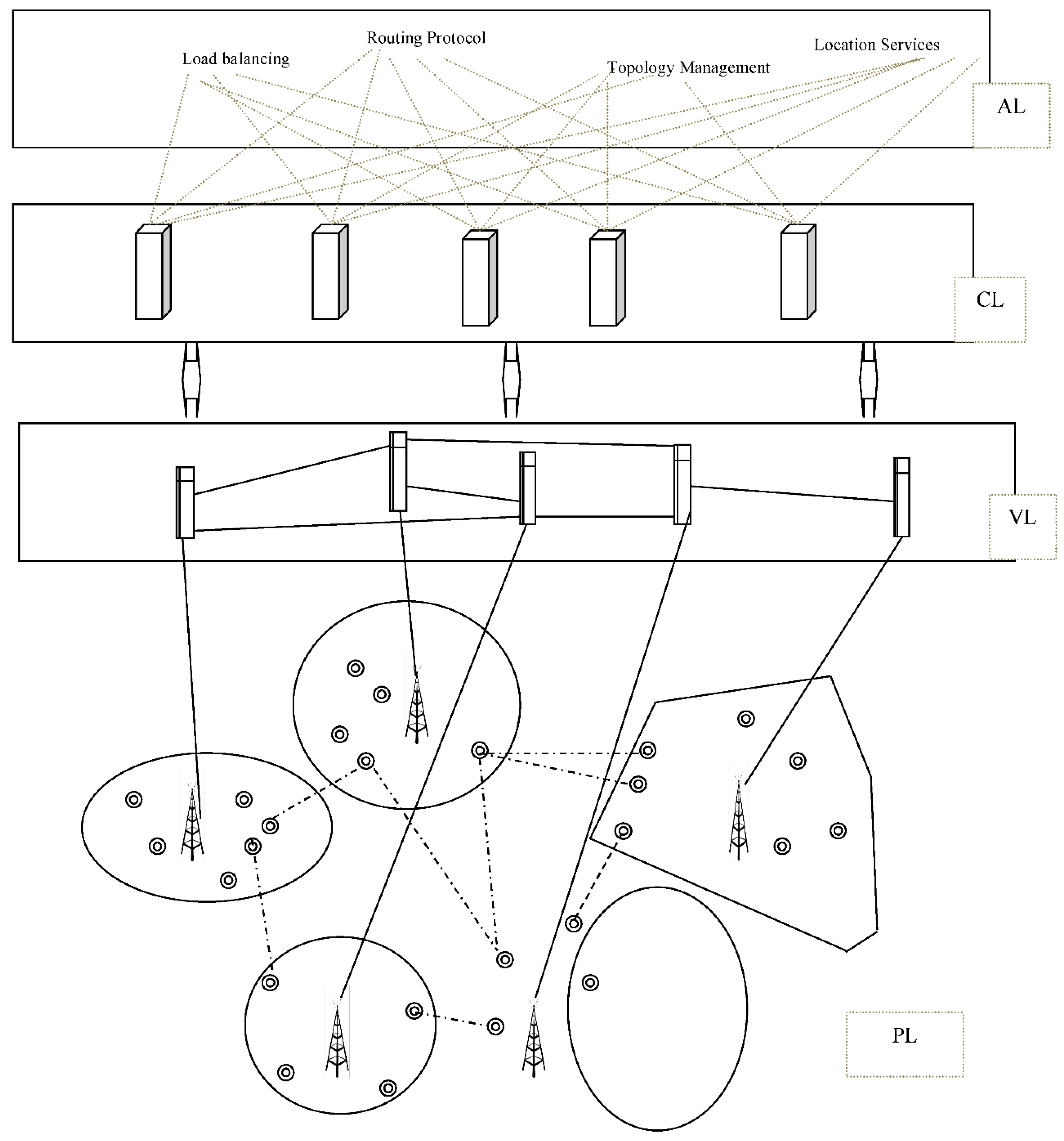
3. Network Framework in SD-EAR
The software defined wireless sensor network framework consists of the following layers, as shown in Figure 2.
3.1. Physical Layer (PL)
This layer consists of several sensor nodes that connect with the SDN controller through OpenFlow protocol [4], and receive relevant flow table information from the SDN controller in that zone. Please note that nodes are divided into certain zones, and each zone is under one unique controller.
3.2. Virtualization Layer (VL)
The key nodes of the sensor network in the physical layer map to virtual key nodes, in order to form the virtual node layer (virtual layer).
3.3. Control Layer (CL)
Controllers in the control layer provide routing, sleep monitoring, and other services to achieve the intelligent management of the WSN. OpenFlow protocol is used to transmit optimum route information to the various nodes that are required to discover the route to some destination. Controllers are capable of generating interrupts to awaken sleepy nodes, and granting sleep requests to worthy or needy nodes.
Depending upon the residual energy of the neighbors of a node, certain nodes are also sent mandatory sleep messages, which are forceful instructions for the node to go to sleep, even though it did not ask for a sleep session. All of these contribute to the reduced energy consumption of the network.
3.4. Application Layer (AL)
The strategy of each application is defined in the application layer. Each application obtains the network status (topology, node status, etc.) from the control layer, and makes decisions according to that strategy. The strategy instructs how services will be provided to the sensor node.
4. SD-EAR in Detail
4.1. Network Model
Network is modeled as a graph G = (V, E) where V represents the set of vertices or sensor nodes, and E represents the set of edges between those nodes. The SDN controller of a zone Zp (1 ≤ p ≤ P; P is the number of all of the zones in the network) consists of the two following tables:
- (i)
- NET-TOPLp
- (ii)
- NODE-STATp
The network topology of zone Zp is stored in the form of the adjacency list in NET-TOPLp. The attributes of this table are:
- (i)
- node-id
- (ii)
- neighbor-list
node-id specifies the unique identification number of a node, whereas neighbor-list is the set of neighbors of the node.
NODE-STATp is a table that contains information about all of the nodes within the zone Zp. The components of this information are:
- (i)
- node-id
- (ii)
- (latitude, longitude) pair
- (iii)
- radio range
- (iv)
- maximum energy
- (v)
- most recent residual energy
- (vi)
- most recent rate of energy depletion
- (vii)
- minimum receive power
- (viii)
- sleep status
- (ix)
- last sleep timestamp
- (x)
- peripheral status
For a node ni, the present geographical position in terms of the (latitude, longitude) pair is specified as (xi, yi), with its radio range being radi. Maximum energy, the last known residual energy, and the rate of battery depletion are denoted as m-eni, r-eni, and depi. Sleep status slpi is 1 if currently ni is sleeping; it is 0 otherwise. τ-sli is the most recent timestamp when ni went to sleep. The peripheral status of ni is given by pphri. It is set to 1 if the radio circle of current node ni is not completely embedded within the area of the zone, i.e., it may have some neighbor belonging to any neighboring zone of Zp. Otherwise, it is set to 0.
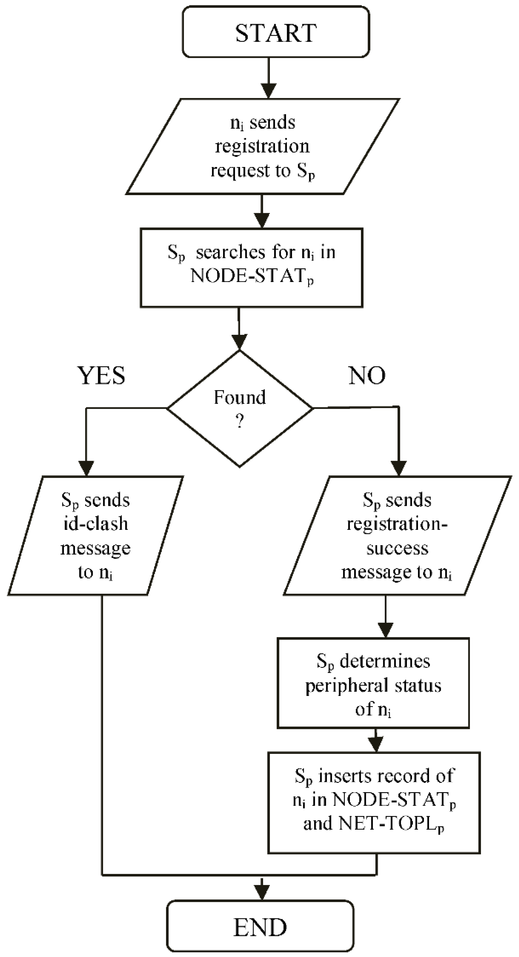
Whenever a node ni starts its operation in the network, it has to first register itself by sending a registration request message to the SDN controller. The components of the registration request are:
- (i)
- message-type-id (0 for registration)
- (ii)
- node-id
- (iii)
- (latitude, longitude) pair
- (iv)
- radio range
- (v)
- maximum energy
Receiving the registration request of ni, the corresponding SDN controller checks the NODE-STATp table to determine whether any entry with same node identifier ni exists within that table. If yes, then an id-clash message will be sent back to ni. The components of an id-clash message are:
- (i)
- message-type-id (1)
- (ii)
- node-id
On the other hand, if no such event of a node identifier clash is detected, then a registration-success message is sent to ni. The attributes of registration-success are the same as id-clash; only the message-type-id is set to 2. After that, the peripheral status of ni is determined. It finds out whether the radio circle of ni is completely embedded within a zone. Three types of zone structures are considered: polygonal, circular, and elliptic. The polygonal structure is the closest to the real life scenario, while the circular structure is the ideal one, where the neighborhood of a node spreads around the node equally in all directions. Please note that the circle is a special kind of ellipse, where both foci are at the same point (the center). Therefore, both circular and elliptic structures have been considered in our simulation. Below, we derive the conditions under which a polygonal, circular, or elliptic zone embeds a radio circle of ni. If the radio circle of ni is completely embedded in the zone, then pphri is set to 0; otherwise, it is 1.
Situation 1: The zone under inspection is polygonal, defined by consecutive vertices (xv+q, yv+q) s.t. 0 ≤ q ≤ Q; the node to be embedded has center (xi, yi) and a radiorange ofradi.
The situation is expressed in Figure 3.
Consider one particular edge E from (xv, yv) to (xv+1, yv+1). The slope m1 of E is mathematically expressed in Equation (1):
m1 = (yv+1 − yv)/(xv+1 − xv)
Let C be the center of the radio-circle of ni. The shortest distance from C to edge E is given by the length of perpendicular from C to E. Assume that the perpendicular drawn on E from C intersects E at point W. Then, the slope m2 of CW is related to m1 as in Equation (2):
m2 = (−1)/m1
CW passes through the point (xi, yi). Based on this, the equation of CW appears in Equation (3):
where:
and:
y = m2 x + b2
m2 = −(xv+1 − xv)/(yv+1 − yv)
b2 = (yi + (xv+1 − xv)/(yv+1 − yv) xi)
The equation of the edge E from (xv, yv) to (xv+1, yv+1) is mathematically expressed in Equation (6):
y = m1 x + b1
s.t. b1 = (xv+1yv − xv yv+1)/(xv+1 − xv)
The coordinates (wx, wy) of the point of intersection of edge E and CW (i.e., the point W) are given by:
wx = (b2 − b1)/(m1 − m2)
wy = (m1 b2 − m2 b1)/(m1 − m2)
If the Cartesian distance between the two points (xi, yi) and (wx, wy) is greater than or equal to radi, then it can be concluded that the radio-circle of ni is embedded within the given zone. The mathematical version of the condition appears in Equation (10):
[{(xi − wx)2 + (yi − wy)2}]0.5 ≥ radi
If such a condition (as in Equation (10)) is satisfied by all of the edges of the polygon, then it can be concluded that the radio circle of ni is completely bounded by the polygonal zone.
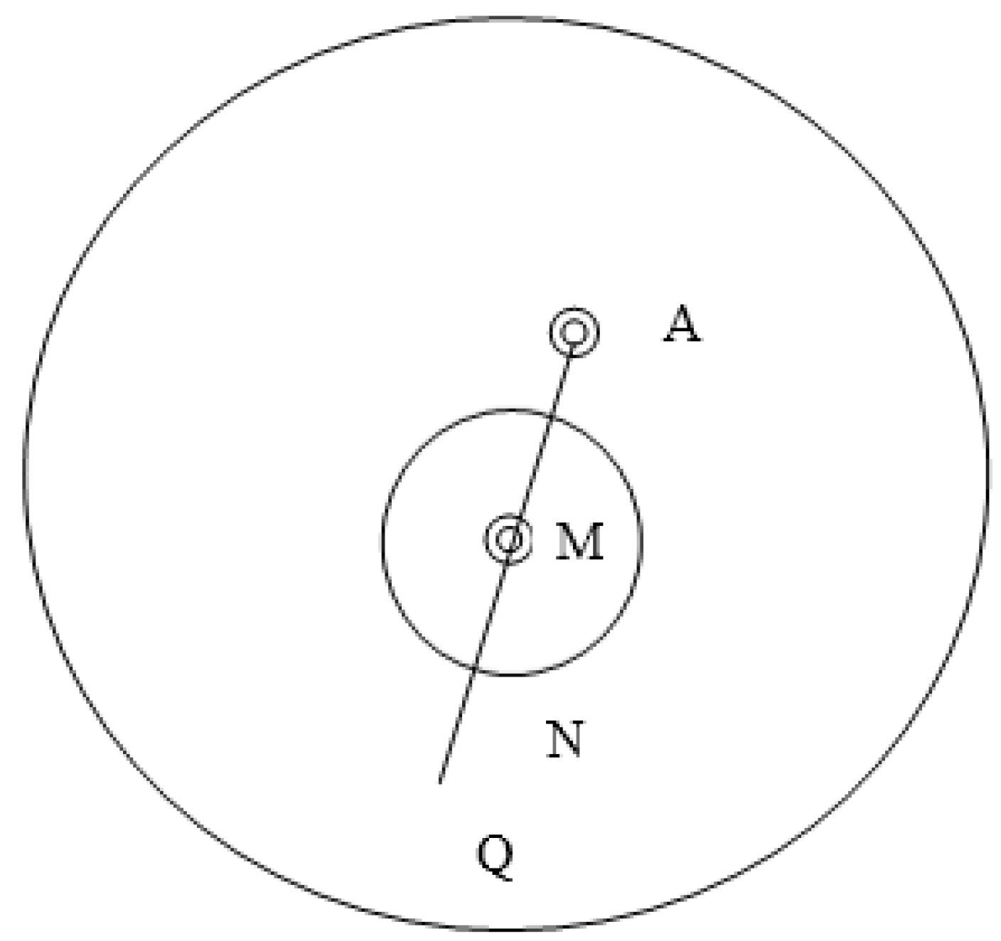
Situation 2: The zone Zp under inspection is circular, defined by cnter (x(Zp), y(Zp)) and radius rad(Zp); the node to be embedded has center (xi, yi) and a radio range radi of ni
The situation is expressed in Figure 4.
In Figure 4, AQ is the radius of the zone; AM specifies the distance between the centers of the zone and node ni. Please note that node ni is positioned at point M. MN is the radio range of the node. The mathematical expressions for AQ, AM, and MN appear in Equations (11)–(13):
AQ = rad(Zp)
AM = [{(x(Zp) − xi)2 + (y(Zp) − yi)2}]0.5
MN = radi
The required conditions for circle embedding appears in Equation (14):
(AQ − AM − MN) > 0
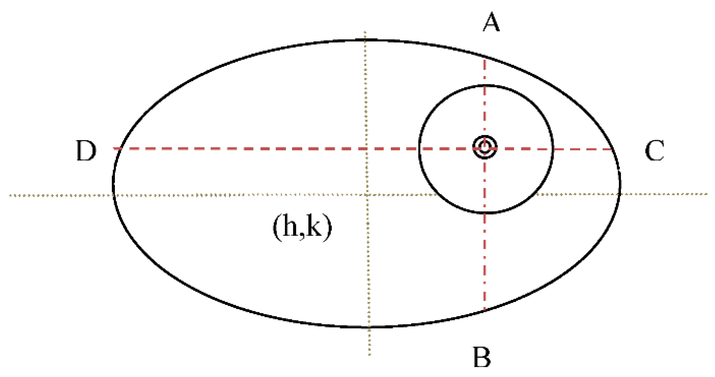
Situation 3: The zone under inspection is elliptic, as defined by Equation (15); the node to be embedded has center (xi, yi) and a radio range of radi.
s.t. a > b. The situation is represented in Figure 5.
(x − h)2/a2+(y − k)2/b2 = 1
The node to be embedded has a center of O (xi, yi) and a radio range of radi. (h,k) is the center of the ellipse. We draw a line AB through O i.e., the center of the radio circle of ni, parallel to the Y axis. The line intersects the ellipse at points A and B. Similarly, we draw a horizontal line through O, i.e., the center of the radio circle of ni, parallel to the X axis. The line intersects the ellipse at points C and D. In order to compute the coordination of A and B, we need to put x = xi into the equation of the ellipse, and calculate the corresponding x coordinates. Similarly, to calculate the coordinates of C and D, we need to put y = yi.
Putting x = xi in the equation of the ellipse:
(xi − h)2/a2+(y − k)2/b2 = 1
Without any loss of generality, the y coordinates of A and B are y1 and y2, respectively, s.t.:
y1 = b{k/b + ((1 − (xi− h)2/a2))0.5}
y2 = b{k/b – ((1 − (xi − h)2/a2))0.5}
Putting y = yi in the equation of the ellipse:
(x − h)2/a2+(yi − k)2/b2 = 1
Therefore, the x coordinates of A and B are either x1 or x2 s.t.:
x1 = a{h/a + ((1 − (yi − k)2/b2))0.5}
x2 = a{h/a –((1 − (yi − k)2/b2))0.5}
OA = |y1 −yi|
OB = | y2 −yi|
OC = |x1 − xi|
OD = |x2 − xi|
If OA < min(b,OB) and OC < min(a,OD) and OC > OA, then the circle is embedded in the zonal ellipse.
After determining the peripheral characteristics of the new node, ni, the SDN controller inserts an entry ENTR(i) corresponding to ni in the NODE-STATp table.
ENTR(i) = (ni, xi, yi, radi, m-eni, m-eni, 0, 0, −1, pphri)
Accordingly, NET-TOPLp is also updated. The information in this table corresponding to ni is (ni, EN(i)) where EN(i) is the set of neighbors of ni in zone Zp itself. A node nj in zone Zp will be the neighbor of ni provided the following condition is true. Generally in sensor networks, the links are bi-directional [2,4,10,15,17]. We have kept this property intact for SD-EAR for simplicity purposes.
radi ≥ ({(xi − xj)2 + (yi − yj)2})0.5
The flowchart for node registration process appears in Figure 6, where node ni is about to start its operation at zone Zp. Let the SDN controller of Zp be denoted as Sp.
4.2. Optimum Route Selection
Whenever a node ni wants to communicate with another node nj, it sends an opt-route-select message to the SDN controller. The attributes of opt-route-select are:
- (i)
- message-type-id (3)
- (ii)
- source-id (ni)
- (iii)
- destination-id (nj)
- (iv)
- timestamp
- (v)
- traversed-zone-list (initially it is {Zp} only; this field is particularly required for inter-zone communication. Whenever opt-route-select arrives at a new zone, the identification number of the new zone is added to the list)
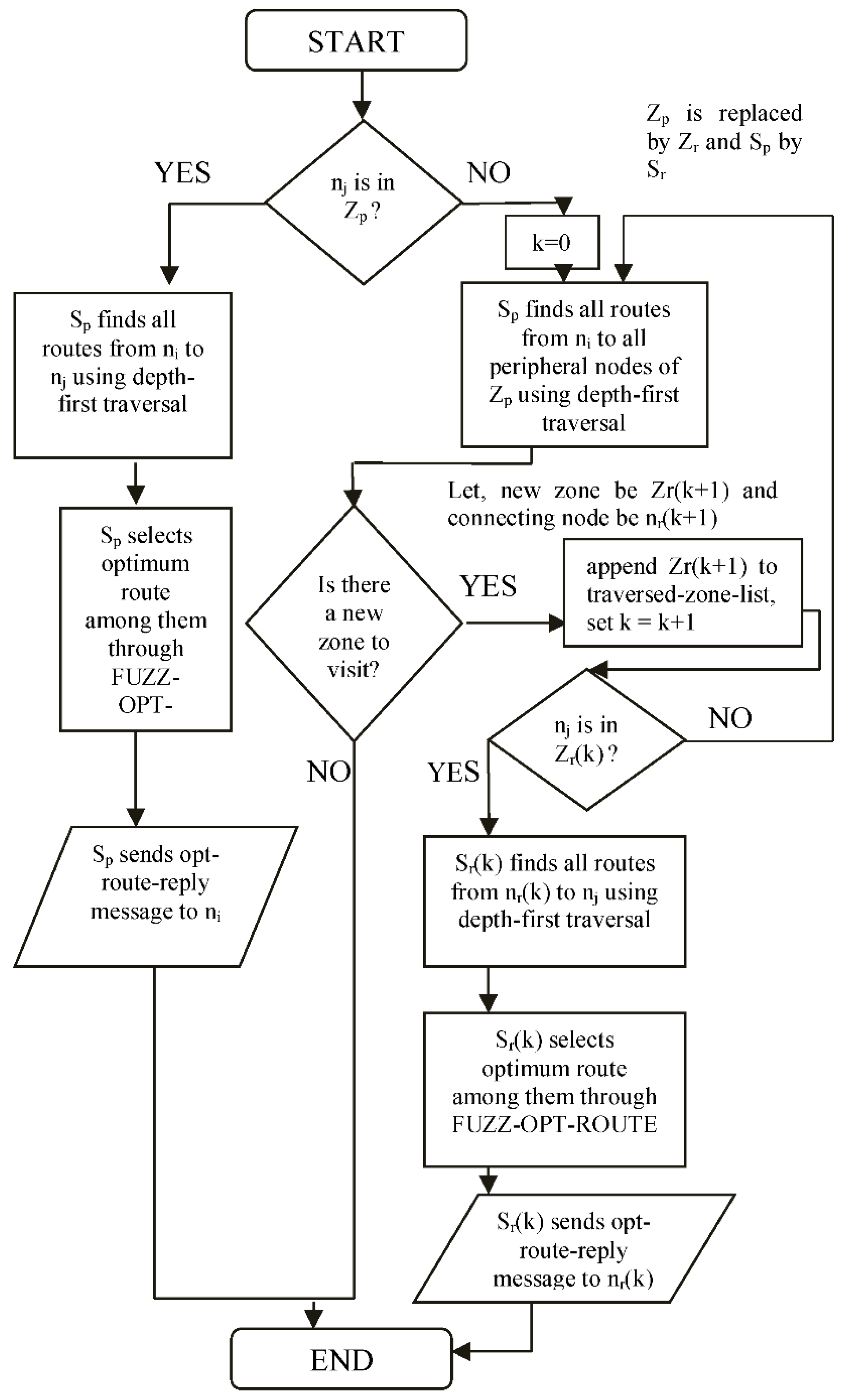
Receiving opt-route-select from ni, the SDN controller of zone Zp checks to see whether destination nj belongs to the same zone or not. This is performed by searching nj in the NODE-STATp table. If nj ∈ extr(NODE-STATp, 1), then an intra-zone route selection is performed; otherwise, an inter-zone route section is performed. Please note that extr(NODE-STATp, 1) is a function that extracts 1-th field from the NODE-STATp table.
After the selection of the optimal route, the SDN controller informs about the chosen sequence of routes to the source of communication in an opt-route-reply message. The attributes of opt-route-reply are:
- (i)
- message-type-id (4)
- (ii)
- source-id (ni)
- (iii)
- destination-id (nj)
- (iv)
- optimal sequence of routers with locations
The flowchart of route discovery appears in Figure 7.
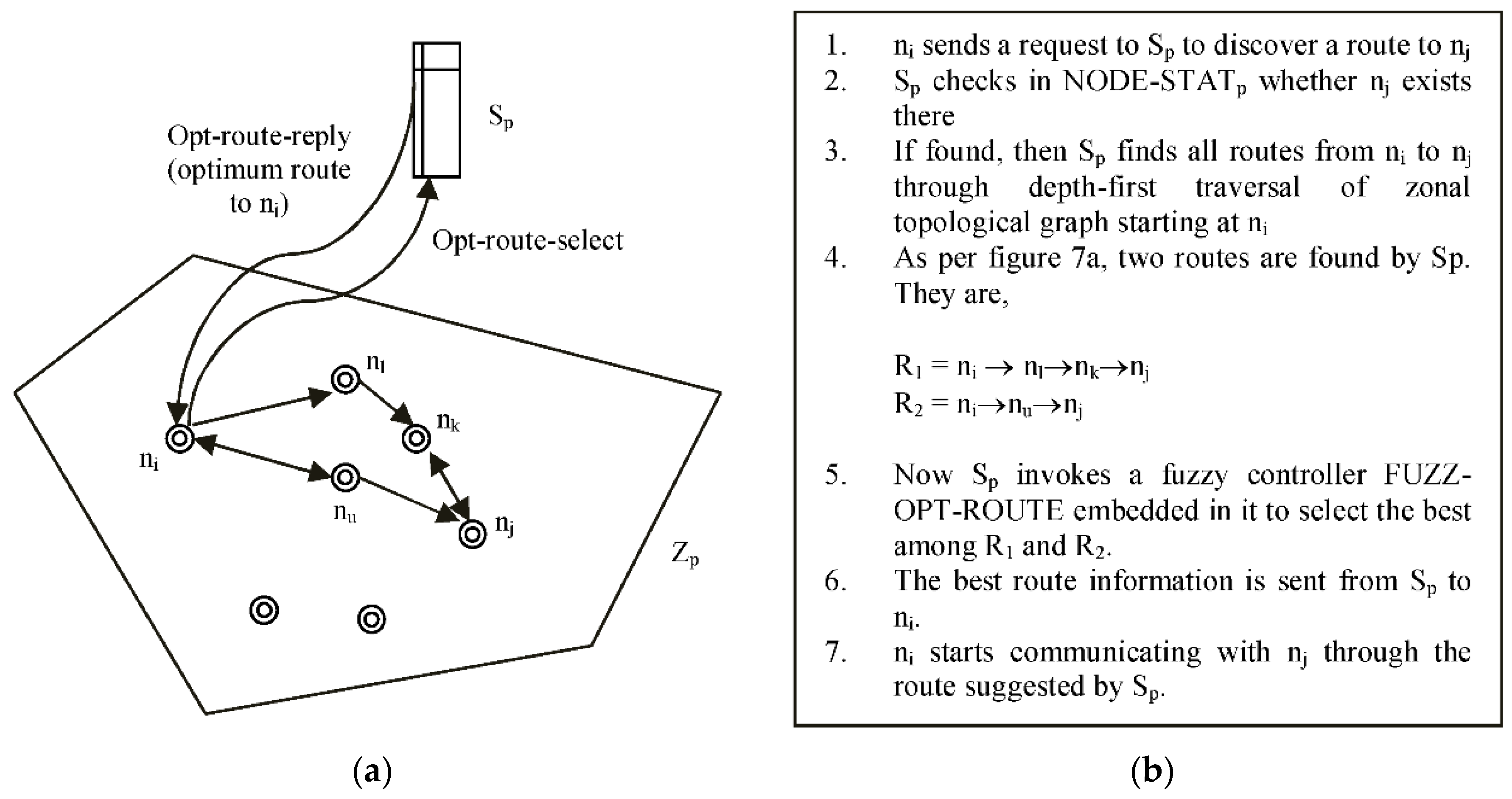
4.2.1. Intra-Zone Route Discovery with Example
If nj belongs to the same zone Zp, then the SDN controller finds all of the routes from ni to nj through the depth first traversal of the graph starting from ni. Among all of the available paths, the optimum one is selected based on a fuzzy controller FUZZ-OPT-ROUTE, which is embedded in the controller. This situation is depicted in Figure 8a, while Figure 8b shows the steps with respect to Figure 8a. Without any loss of generality, we consider a polygonal zone.
Intra-zone communication is loop-free
The communication inside a zone is completely controlled by the SDN controller of the zone, which is aware of the topology of the entire zone. While discovering the optimum route between two nodes inside a zone, the controller of that zone applies depth-first traversal, which automatically eliminates loops. Therefore, intra-zone communication is loop-free.
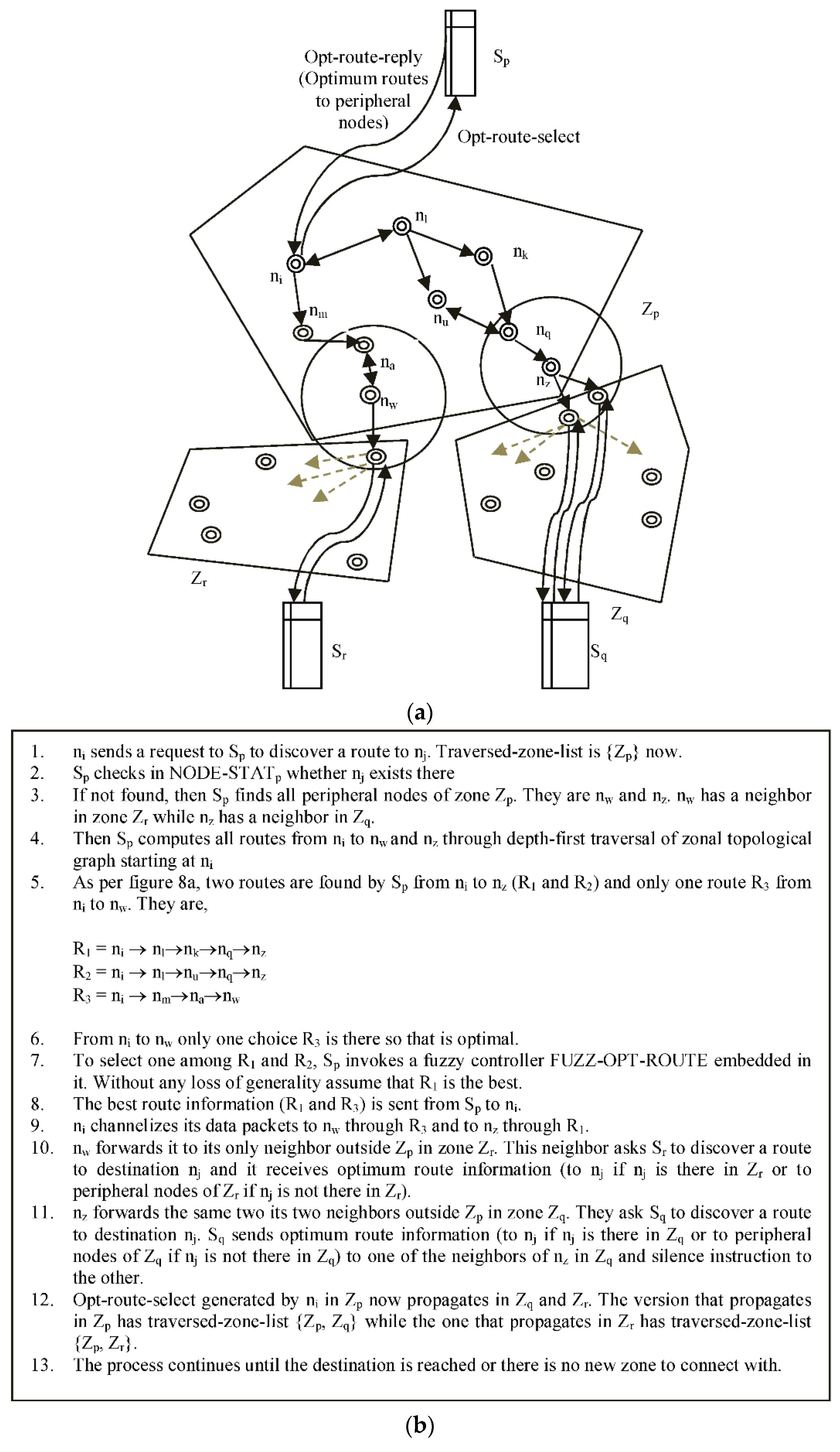
4.2.2. Inter-Zone Route Discovery with Example
If destination nj doesn’t belong to the same zone Zp as source ni, then the SDN controller Sp finds all of the routes from ni to all of the peripheral nodes of Zp through the depth-first traversal of the graph, starting from ni.
The situation can be seen in Figure 9a, while Figure 9b shows the steps of optimum route selection in case of inter-zone route discovery. In this case, opt-route-select has to be propagated to neighbors Zp, too. In that case, the SDN controller finds the routes from ni to all of the nodes nq ∈ extr(NODE-STATp,1) s.t. extr(NODE-STATp,9) = 1. nq forwards the opt-route-select to all of the neighbors that do not belong to Zp.
The neighbors of nq ask the SDN controllers of their respective zones to find out routes to all of the nodes in its neighbor list. Communication in neighbor zones may be again intra-zone or inter-zone. Please note that SDN controllers belonging to multiple zones do not directly communicate with each other. Rather, the peripheral nodes of various zones communicate with each other. Inter-zone communication is actually a collection of multiple intra-zone communications.
In inter-zone communication, if a SDN controller Sq of a zone Zq receives opt-route-select from more than one of its nodes corresponding to the same destination, then it sends opt-route-reply to the one with the highest residual energy (nb), while the others (say nc) are instructed to remain silent.
The attributes of this silence message are as follows:
- (i)
- message-type-id (5)
- (ii)
- source-id (ni)
- (iii)
- destination-id (nj)
- (iv)
- router-id (nc)
Inter-zone communication is loop-free
The traversed-zone-list field contains the sequence of zones that one particular opt-route-select message has traversed. Therefore, one opt-route-select message cannot be propagated within a zone more than once. This avoids loops. Moreover, intra-zone communication from a node to the peripheral nodes of the zone are definitely loop-free, because they are determined by the SDN controller of that zone by dint of the depth-first traversal of the zonal topological graph. This technique is loop-free, as already mentioned, in case of intra-zone communication.
INPUT PARAMETERS OF FUZZ-OPT-ROUTE
reft(R) or residual energy effect of route R
This parameter indicates how the residual energy of nodes belonging to R influence the performance of the route. It is mathematically modeled in Equation (23):
such that
start(R) and end(R) specify the source and destination nodes, respectively, in route R. If, for one particular route, no router nodes are there, then (minr-enk) among all of the routers nk∈R, will be 0.
f-en1(R) = 1 − {1/(min r-enk + 2)}
nk ∈ R
k ≠ start(R) and
k ≠ end(R)
f-en2(R) = 1 − {α(R)/(∑r-enk + 2)}
nk ∈ R
nk ∈ R
From the formulation in Equation (23), it is evident that reft(R) ranges between 0 and 1. It is close to 1 if the minimum and average residual energies of R are high. The high values of this parameter are beneficial for the performance of the route. In Equation (24), 2 is added to the denominator to avoid a zero value when the min r-enk among all of the routers nk ∈ R is 0. Similarly, in Equation (25), 2 is added to the denominator to avoid a zero value when r-enk of all of then k ∈ R is 0. If any one of the f-en1(R) and f-en2(R) is 0, then the effect of the other one will be completely eliminated, which is undesirable.
trim(R) or the transmission energy impact of route R
Transmission energy impact depends on the minimum received power of the nodes in route R and the maximum distance between consecutive nodes. With the increase in this distance and the minimum received power of the successors (by successor we mean all of the nodes except the source) in R, the transmission cost increases, while trim(R) decreases.
succ(nk, R) is the successor node of nk in R. mrpw(nv) is the minimum received power of node nv. dist(na, nb) specifies the Cartesian distance between nodes na and nb.
trim(R) = √(f-recv1(R) × f-recv2(R))
f-recv1(R) = (1 − ∑mrpw(succ(nk, R))/(α(R) × (max mrpw (nv) + 1))
nk ∈ R nv ∈ Zp
f-recv2(R) = max {1, dist(nk, succ(nk, R))}
nk ∈ R
nk ∈ R nv ∈ Zp
f-recv2(R) = max {1, dist(nk, succ(nk, R))}
nk ∈ R
From the formulation in Equation (26), we can see that trim lies between 0 and 1. High values of it contribute to improve the performance of R.
neff(R) or node efficiency in R
The node efficiency in a path will be high, as most of the nodes are awake, and alternatives are available to sleeping nodes (if any). A node nu will be an alternative to another node nv w.r.t. route provided the following conditions are satisfied:
nu ∉ R if nv ∈ R
EN(u) ≥ EN(v)
{r-enu/(depu + depv)} ≥ (r-env/depv)
Condition (27a) specifies that nu should not belong to any live communication route passing through nv. Condition (27b) says that nv must have all of the neighbors of nu as its neighbors. The condition (27c) indicates that the additional forwarding load from neighbors of nu should not reduce the lifetime of nv below the lifetime of nu. If nu is an alternative of nv, then nu ∈ alt(v) where alt(v) is the set of all of the alternatives of nv.
The mathematical formulation of neff appears in Equation (28):
neff(R) = (eff1(R) × eff2(R))0.5
eff1(R) = (1 − β(R)/α(R))
eff2(R) = 1 − [1/{(∑alt(k)/α(R)) + 2}]
nk ∈ R
k ≠ start(R) and
k ≠ end(R)
From Equation (28), it is evident that the efficiency of a route increases with the number of awake nodes and the number of alternatives to sleepy nodes. neff lies between 0 and 1. High values of it indicate the efficiency of the associated route.
FUZZY RULE BASES OF FUZZ-OPT-ROUTE
All of the input parameters of the FUZZ-OPT-ROUTE are divided into four equal ranges between 0 and 1. The ranges and corresponding fuzzy premise variables are as follows:
- (i)
- 0–0.25 (LOW or ‘L’ is short)
- (ii)
- 0.25–0.50 (SATISFACTORY or ‘S’ in short)
- (iii)
- 0.50–0.75 (HIGH or ‘H’ in short)
- (iv)
- 0.75–1.00 (VERY HIGH or ‘VH’ in short)
The rule bases of this fuzzy controller appear in Table 1 and Table 2. Table 1 combines reft and trim, producing temporary output temp1. Both of these parameters are assigned equal weight, since both are equally important in determining the efficiency of the route. If a node has high residual energy but suffers from huge energy consumption due to the long distance from its successor in a communication path, then the energy efficiency of a path greatly reduces. Therefore, temp1 = min (reft, trim) in Table 1. Examples are: reft = H, trim = S, temp1 = S; reft = S, trim = L, temp1 = L; and reft = VH, trim = S, temp1 = S. The composition of temp1 and neff is presented in Table 2. Then eff of a route increases with an increased number of awake nodes and alternatives to sleepy nodes, if any. temp1 is given more weight than neff, only because a huge number of awake nodes will not do. They need to have high residual energy and a low transmission energy requirement in each hop so that the route can last for a long time. The influence of neff increases when temp1 is not high. Hence, in Table 2, when temp1 = L or S, the output opt-performance = min(temp1, neff). On the other hand, when temp1 = H or VH, small values of neff are capable of reducing it to some extent. For example, when temp1 = H and neff = L, opt-performance = S. The optimal path is the one that produces the best opt-performance. In the case of multiple optimal options, any one with the least weight is elected as optimal. Weight(R), that is, the weight of an optimal route R, is mathematically formulated below in Equation (29):
γ(R) specifies the total number of sleepy nodes in R, while α(R) is the total number of nodes in R. If still a tie remains, then any one is chosen for communication.
Weight(R) = (α(R) × (γ(R) + 1))
4.2.3. Example of Optimum Path Selection
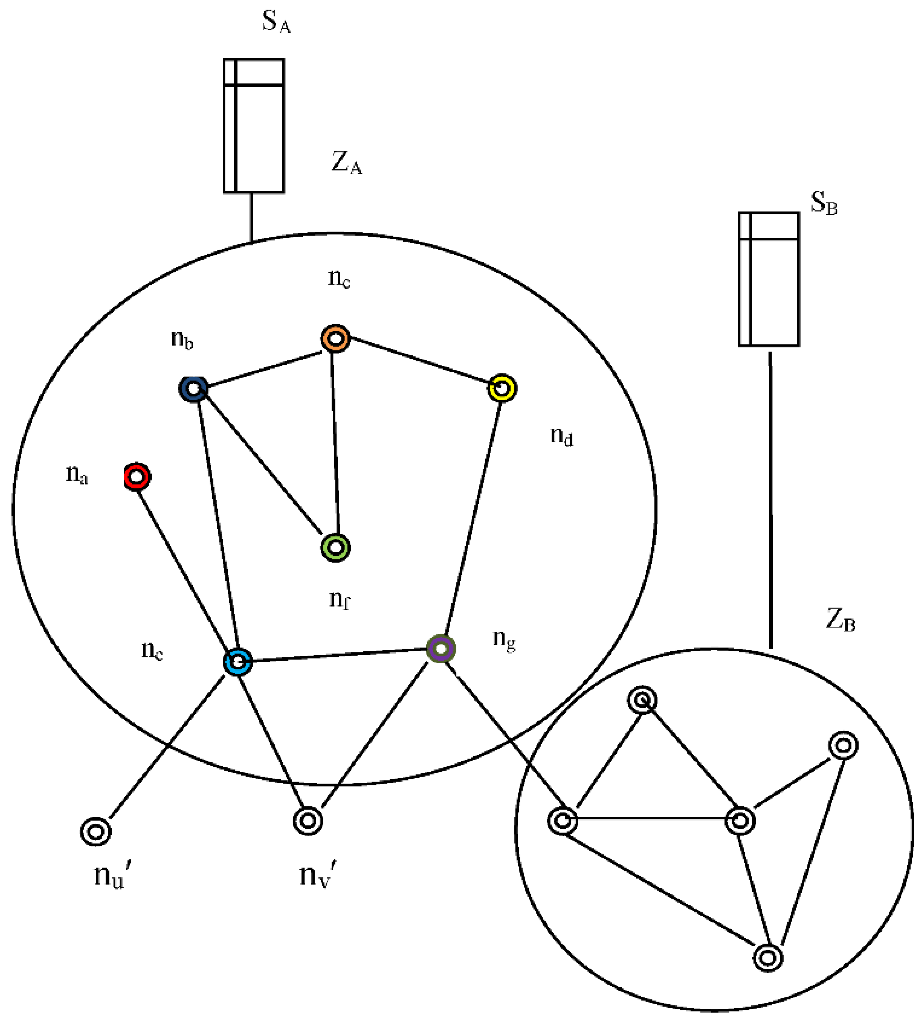
Table 3 specifies all of the node ids in Figure 10 along with their descriptions. Based on these assumptions, we are about to find out the optimal route from nb to nd at current timestamp 100. The significance of all of the symbols used in Table 3 have been mentioned earlier in this section. For the purpose of simplicity, we have assumed that all of the links are bi-directional. The latitude and longitudinal positions are given in Table 3. It is seen from Figure 10 that na is directly connected to ne only, while ne is directly connected to na, nb, ng, nu′, and nv′. Among them, nu′ and nv′ are out of ZA. So, EN(a) = {ne} and pphra = 0, since ne∈ ZA. On the other hand, EN(a) = {na, nb, ng, nu′, nv′} and pphre = 1, since nu′, nv′ ∉ ZA. Similarly, the EN and pphr of other nodes can be computed. Other attribute values are assumed. The performances of different routes from nb to nd are calculated in the FUZZ-OPT-ROUTE of SDN controller of ZA.
The different routes from nb to nd obtained through a depth-first traversal of topology of ZA, are as follows:
- (i)
- R1: nb→nc→nd
- (ii)
- R2: nb→nc→nd
- (iii)
- R3: nb→nc→nf→nd
- (iv)
- R4: nb→nf→nc→nd
- (v)
- R5: nb→ ne→ ng→nd
Performance of R1
reft(R1) = [{1 − 1/(20 + 2)} {1 − 3/(3 + 20 + 20 + 2)}]0.5 = 0.9438
trim(R1) = [{1 − (2 + 1)/(3 × 4)}/max{20.5, 0.50.5}]0.5 = 0.7282
neff(R1) = [{1 − 0/3} (1 − 1/(1 + 2))]0.5 = 0.8176
After fuzzification, the fuzzy premise variables corresponding t reft(R1), trim(R1), andneff(R1) become VH, H, and VH, respectively. Their combination, according to Table 1 and Table 2, is VH.
Hence, opt-performance = VH
Performance of R2
reft(R2) = [{1 − 1/(25+2)} {1 − 3/(3 + 25 + 20 + 2)}]0.5 = 0.9509
trim(R2) = [{1 − (1 + 1)/(3 × 4)}/max{80.5, 0.50.5, 1}]0.5 = 0.5426
neff(R2) = [{1 − 0/(3)} (1 − 1/(0 + 2))]0.5 = 0.7071
After fuzzification, fuzzy premise variables corresponding t reft(R2), trim(R2), andneff(R2) become VH, H, and H. Their combination, according to Table 1 and Table 2, is VH.
Hence, opt-performance = H
Performance of R3
reft(R3) = [{1 − 1/(20 + 2)} {1 − 4/(3 + 20 + 25 + 20 + 2)}]0.5
i.e., reft(R3) = 0.94845
trim(R3) = [{1 − (2 + 1 + 1)/(4 × 4)}/max{20.5, 0.50.5}]0.5 = 0.866
nf is sleeping. We need to search for alternatives of nf. Only nc has the same set of neighbors as nf. However, nc belongs to this route R3 itself. So, nc cannot be an alternative to nf. So, nf has no alternative:
neff(R3) = [{1 − 1/(3 + 1)} (1 − 1/(0 + 2))]0.5 = 0.61237
After fuzzification, the fuzzy premise variables corresponding t reft(R3), trim(R3), and neff(R3) become VH, VH, and H. Their combination, according to Table 1 and Table 2, is VH.
Hence, opt-performance = VH
Performance of R4
reft(R4) = [{1 − 1/(20 + 2)} {1 − 4/(3 + 20 + 25 + 20 + 2)}]0.5
i.e., reft(R4) = 0.94845
trim(R4) = [{1 − (2 + 1 + 1)/(4 × 4)}/max{80.5, 20.5, 0.50.5}]0.5 = 0.5147
nf is sleeping. We need to search for alternatives of nf. Only nc has same set of neighbors as nf. However, nc belongs to the route R3 itself. So, nc cannot be an alternative to nf. So, nf has no alternative.
neff(R4) = [{1 − 1/(3 + 1)} (1 − 1/(0 + 2))]0.5 = 0.61237
After fuzzification, the fuzzy premise variables corresponding t reft(R4), trim(R4), and neff(R4) become VH, H, and H. Their combination, according to Table 1 and Table 2, is H.
Hence, opt-performance = H
Performance of R5
reft(R5) = [{1 − 1/(20 + 2)} {1 − 4/(3 + 20 + 30 + 20 + 2)}]0.5
i.e., reft(R5) = 0.9498
trim(R5) = [{1 − (3 + 1 + 1)/(4 × 4)}/max{1050.5, 1.250.5, 76.56250.5}]0.5
i.e., trim(R5) = 0.229
In this path, only ng is sleeping. We need to search for alternatives of ng. However, no node in zone ZA has the same set of neighbors as ng. So, ng has no alternative.
neff(R5) = [{1 − 1/(3 + 1)} (1 − 1/(0 + 2))]0.5 = 0.61237
After fuzzification, the fuzzy premise variables corresponding t reft(R5), trim(R5), and eff(R5) become VH, L, and H, respectively. Their combination, according to Table 1 and Table 2, is L.
Hence, opt-performance = L
R1 and R4 both have performance VH. Therefore, we compute the weight of these paths.
Weight(R1) = 3 × 1 = 3
Weight(R4) = 4 × 2 = 8
Therefore, R1 is chosen as optimal.
4.2.4. Sleeping Strategy
Whenever a node ni wants to go to sleep, it needs to ask for permission from the SDN controller of that zone. It gets a sleep grant provided that the following conditions are true:
- (i)
- (r-eni/depi) < TH where TH is a threshold.
- (ii)
- If ni is part of any live communication route, then it must have at least one valid alternative. The strategy of computing an alternative is present in (27a)–(27c).
Also, there is one forceful sleep grant mechanism. When all of the neighbors of a node ni are sleeping, then ni is instructed by the SDN controller in that zone to go to sleep if it does not want to transmit anything. It has practically no reason to listen to the network, because it has no way of receiving any traffic.
The attributes of a sleep request are:
- (i)
- message-type-id (5)
- (ii)
- node-id (ni)
Similarly, the attributes of a sleep grant are:
- (i)
- message-type-id (6)
- (ii)
- node-id (ni)
5. Simulation Experiments
5.1. Simulation Environment
This experiment is based on SDN and the IEEE 802.15.4 protocol for wireless sensor networks. The network emulator for the framework is Mininet [30], and the controller is Floodlight [31]. Floodlight runs on a server with an AMD Opteron processor 6348 and 16 GB memory. The server is installed with Linux kernel version 2.6.32. Mininet runs on a separate server, and the servers are connected by a 10 Gbps Ethernet network. Details appear in Table 4.
The simulation metrics are:
- (i)
- Overall Message Cost (OMC)—This is a summation of messages sent by all of the nodes in the network. msgk denotes the total number of messages sent by nk throughout the simulation period.OMC = ∑msgk
nk ∈ NW - (ii)
- Overall Energy Consumed (OEC)—This is a summation of energy consumed in all of the nodes in the network.OEC = ∑ (m-enk − r-enk)
nk ∈ NW - (iii)
- Network Throughput (NT)—This is the percentage of data packets that were successfully delivered to their respective destinations. t-p is the number of packets transmitted throughout the communication session, and d-p is the number of packets successfully delivered to their destinations throughout the simulation run.NT = (d-p/t-p) × 100
- (vi)
- Average Delay (AD)—This is a summation of delay faced by all of the packets in the network, divided by the number of packets transmitted. PAC is the set of all of the packets transmitted throughout the simulation. d-l(pac) denotes the delay suffered by packet PAC:AD = ∑ d-l(pac)/|PAC|
pac ∈ PAC - (v)
- Percentage of alive nodes per established communication session (PALCS)—This isthe summation of the number of alive nodes (ALVN(CS)) in session CS multiplied by 100 anddivided (by total number of nodes in optimal route in the same session × total number of established sessions). SES is the set of all of the sessions established throughout the simulation time. route(CS) is total number of nodes in an optimal route in session CS.PALCS = ∑ (ALVN(CS) × 100)/(|SES| × route(CS))
CS ∈ SES
5.2. Simulation Results
Graphical comparisons of SD-EAR with its state-of-the-art competitors LEACH, SPIN, SD-WSN1, SD-WSN2, and SD-WSN3, are presented in Figure 11, Figure 12, Figure 13, Figure 14, Figure 15, Figure 16, Figure 17, Figure 18, Figure 19 and Figure 20.
5.2.1. SD-EAR versus LEACH, SPIN
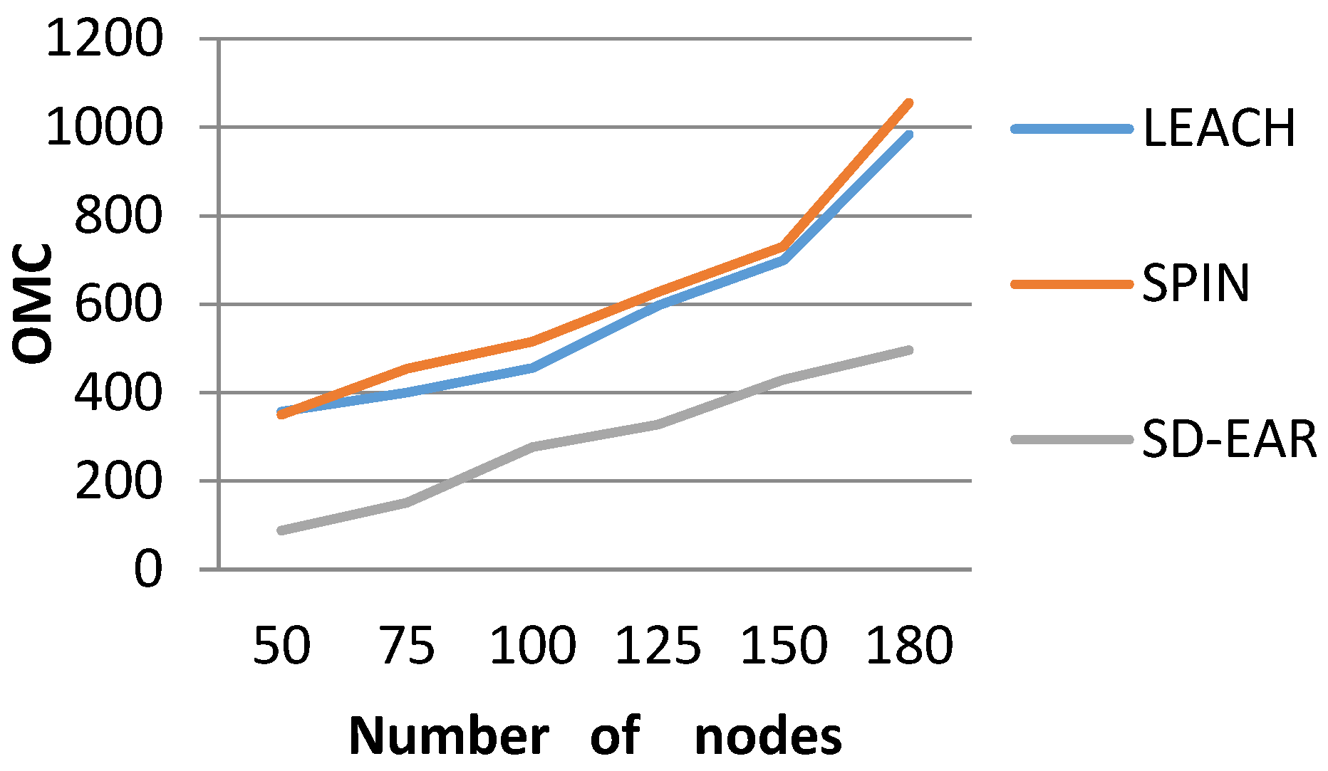
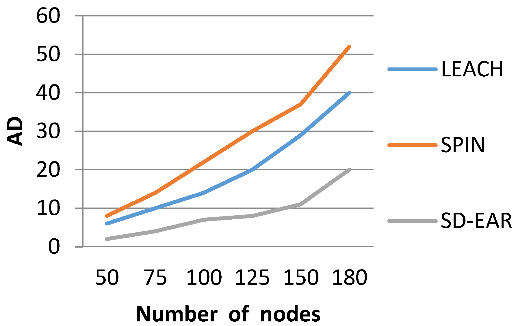
LEACH divides the sensor network into multiple clusters. The technique for electing a cluster-head is the main source of energy efficiency here. If a node has already played the role of a cluster-head in several runs, then its chance of becoming a cluster-head in the next run again reduces greatly. This encourages the rolling of cluster-heads by the balancing load. However, LEACH does not consider the location of sensor nodes [35,36,43] and therefore, certain cluster members may stay very far from the cluster-head. So, the energy consumed by the cluster-head in transmitting a message to those members that are located far, increases substantially. Also, LEACH applies Dijkstra’s shortest path algorithm to select the optimum path [43]. The authors would like to state here that shortest path, in most cases, is not the most energy-efficient one. Hence, the performance improvement produced by SD-EAR over LEACH is noteworthy. This is evident in Figure 11, Figure 12, Figure 13, Figure 14 and Figure 15.
SPIN [38] is also a very important energy-efficient protocol that broadcasts metadata, which is data about data. If a neighbor develops interest about actual data after receiving the metadata, only then is data sent to it. The energy efficiency in SPIN arises from the size of the metadata being much less than the size of the actual data, and the actual data is sent to a subset of neighbors instead of all of the neighbors, as in an ordinary broadcast.
On the other hand, in SD-EAR, the broadcasting of an opt-route-select is not performed, not even in inter-zone communication. Actually, in the inter-zone route discovery, opt-route-select is at most multicast to all of the peripheral nodes, as well as also through energy-efficient paths, as instructed by the SDN controller in that zone. Those routes do not break easily, and the requirement of route-rediscovery arises significantly less in our proposed protocol, which reduces the message cost in SD-EAR compared with LEACH and SPIN, as seen from Figure 11.
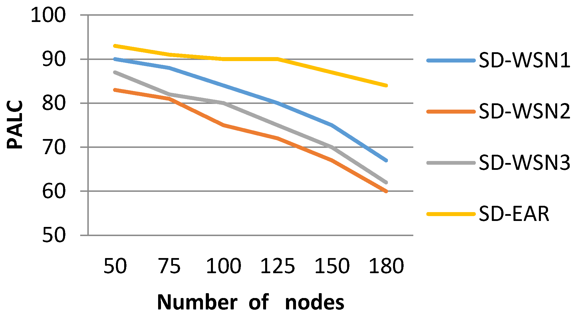
5.2.2. SD-EAR versus SD-WSN1, SD-WSN2 and SD-WSN3
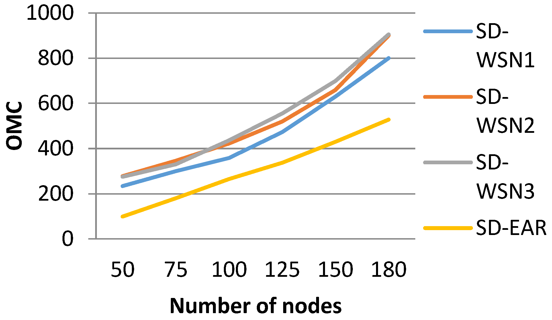
SD-WSN1 applies either a proactive or reactive routing policy depending upon the total number of nodes in the network. If the number of nodes is low, then proactive routing is applied, where the identifiers of successors in optimum paths to various destinations are stored in routing tables. This does not require route discovery before each communication session, and saves energy by eliminating the broadcast operation during route discovery when the number of nodes is low [12]. However, when the number of nodes becomes high, routing table storage becomes inefficient; also, keeping track of stale routes is difficult. In that case, it applies reactive routing and the corresponding protocol is ad hoc on demand distance vector routing, or AODV. Among the various paths through which the route-request arrives at its destination from the source, the path with the least number of hops is elected as optimal. No energy efficiency is applied during optimum route selection. Also, there is no provision of giving rest to exhausted nodes. SD-WSN1 is capable of avoiding the broadcasting of route-request only when number of nodes is low enough.
SD-WSN2 [20] is concerned with only the optimum placement of energy transmitters. Energy transmitters provide energy to the nodes when they suffer from a shortage of charge. Please note that the recharging of nodes is less frequent than the initiation of new communication sessions. SD-WSN3 [21] selects a few control nodes among all of the nodes in the network. These nodes assign task to others, depending upon the residual energy. However, here, the authors want to humbly state that residual energy is not the only criteria. A node ni may have higher residual energy (say for example, 50 mj) than another node nj (30 mj), but this does not mean that ni will live longer. It depends on the energy depletion rate or packet-forwarding load. If we assume that the energy depletion rate of ni is 10 mj/s and that of nj is 2 mj/s, then the residual lifetime of ni and nj are 5 s and 15 s, respectively.
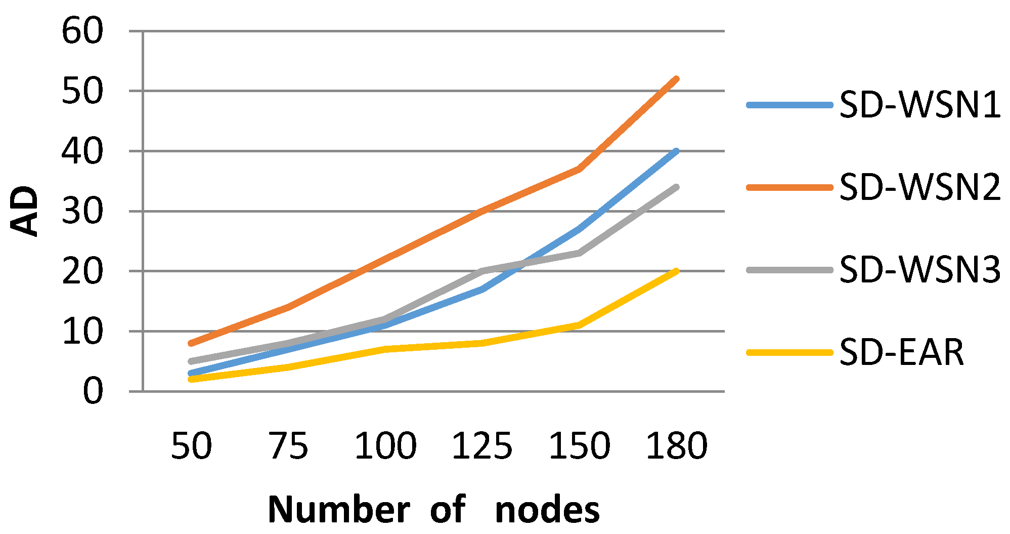
SD-EAR considers different aspects of energy efficiency, such as residual energy, the energy depletion rate, the distance between consecutive nodes in a route, the number of sleeping nodes, and their alternatives. All of these criteria enable the establishment of long-lasting routes and the requirement of route rediscovery reduces up to a greater extent than SD-WSN1, SD-WSN2, and SD-WSN3. SD-EAR converts the broadcasting of a route-request to multicasting opt-route-select to only the peripheral node group whose member cardinality is generally much smaller than the total number of nodes in a zone. Therefore, SD-EAR suffers from much less message cost than its state-of-the-art software defined competitors, as seen in Figure 16.
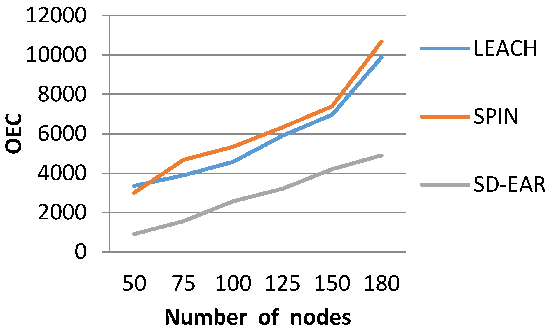
Overall Energy Consumed (OEC)
The most important aspect of SD-EAR is that it completely eliminates broadcasting during route discovery. This saves a huge number of messages. Also, route selection strategy in SD-EAR is extremely energy-efficient. The eligibility of a route depends upon the pairwise distance between consecutive nodes, the number of alternatives, the residual energy, the rate of energy depletion, etc. A sleeping strategy is proposed too, that examines the need of sleep of a node after receiving a sleep request. A sleep is granted by the SDN controller if the zonal topology has a provision of its alternative, so that the alive communication session does not face any link breakage. The provision of forceful sleep instruction from the SDN controller to different nodes is possible in SD-EAR. Link breakages are repaired proactively. All of these things greatly reduce the overall energy consumption, or OEC, in SD-EAR compared with its competitors. This is seen in Figure 12 and Figure 17. However, as the number of nodes increases, the OEC also increases for all of the protocols, but still, the growth is least steep for SD-EAR.
Percentage of alive nodes per established communication session (PALCS)
Routing protocol in SD-EAR balances the load between various nodes in the network and greatly reduces the overall energy consumption. The reduction in message cost cuts down on the energy consumption in various nodes. Moreover, balancing the load prohibits overwhelming differences between the residual energy of various nodes. This increases the number of alive nodes in different communication sessions, as shown in Figure 15 and Figure 20.
Network Throughput (NT)
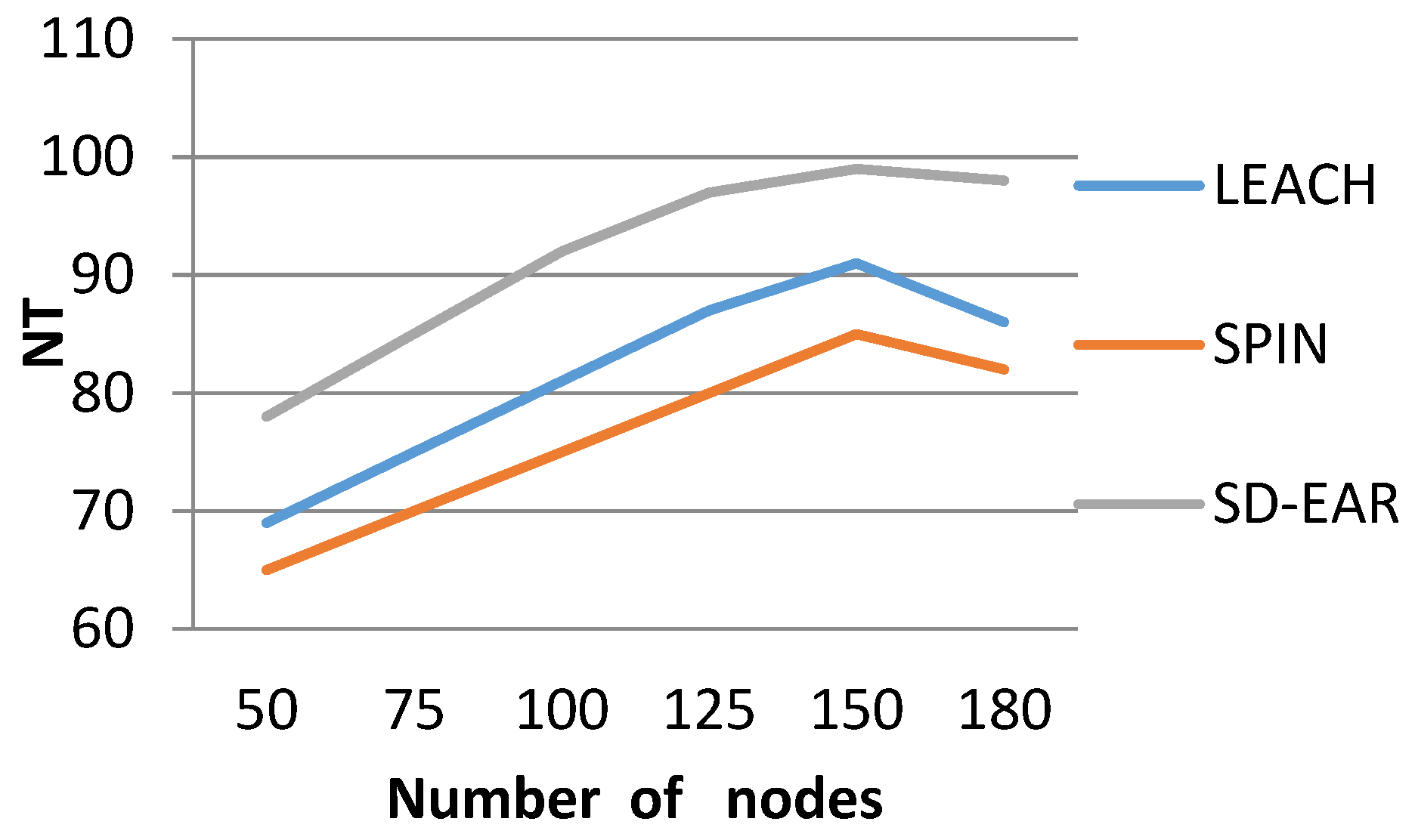
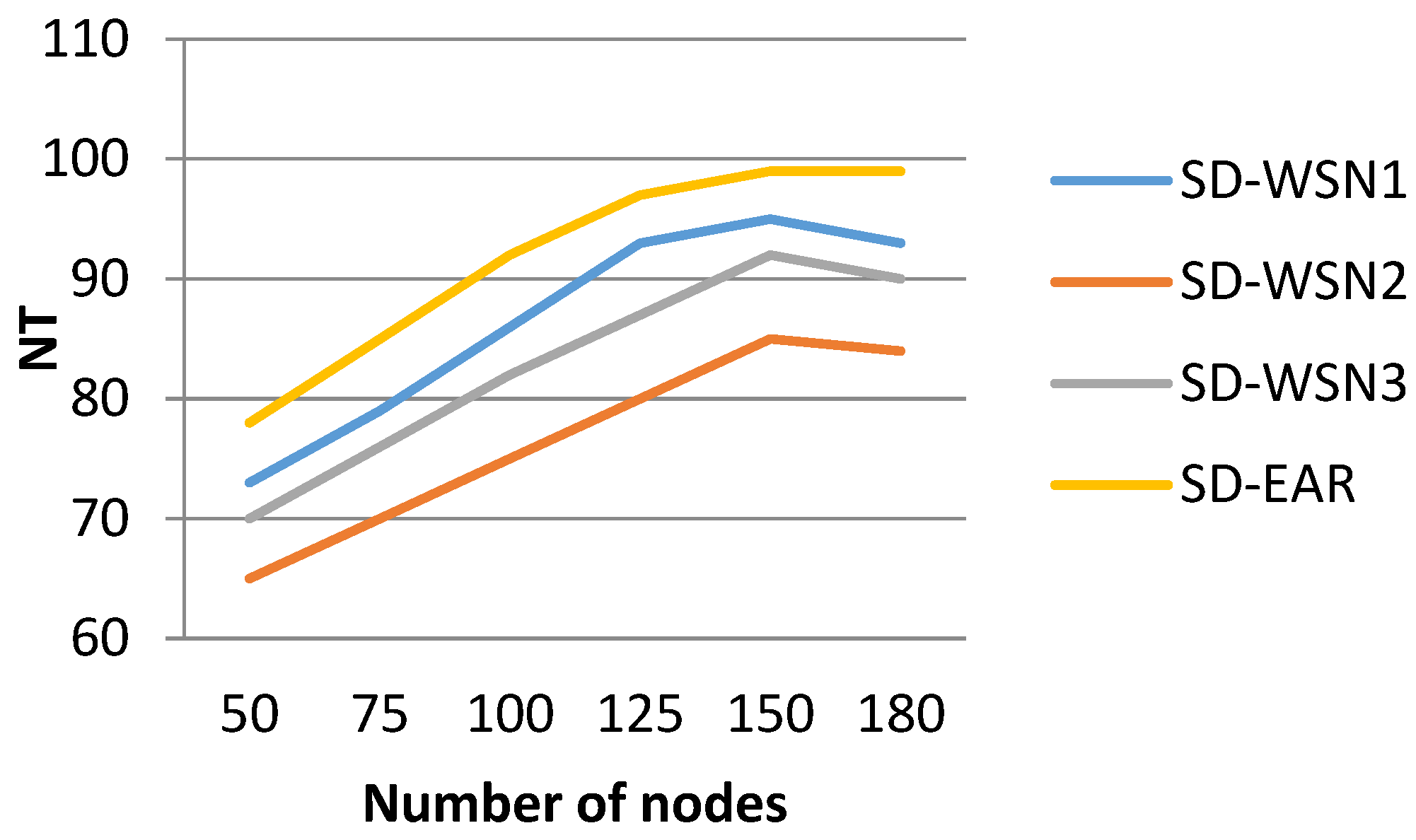
We all know that if the number of messages in the network increases upto a great extent, then it gives rise to a huge amount of message contention and collision, yielding a high rate of packet loss. Since the competitors of SD-EAR suffer from much more message overhead than our proposed protocol SD-EAR, the network throughput produced by SD-EAR is much higher than others, as shown in Figure 13 and Figure 18. It is seen in the figures that for all of the protocols, network throughput initially increases with the number of nodes; then, it starts decreasing. The reason is that with the increase in the number of nodes, more links are formed, and more data packets are delivered to their respective destinations. However, when the network becomes saturated with nodes, message contention and collision increases, reducing network throughput.
Average Delay (AD)
We have already mentioned that broadcasting for route-request is completely eliminated in SD-EAR. Therefore, the delay in route discovery is reduced by a great extent in our proposed protocol. Moreover, link breakages are also repaired proactively. This saves the time span that would have been required to identify a broken link and initiate route-rediscovery to repair the link. Therefore, the average delay in SD-EAR is much smaller than that of its competitors, as shown in Figure 14 and Figure 19.
6. Conclusions
This article presents a software defined wireless sensor framework where the network is divided into multiple clusters or zones, and each zone is controlled by an SDN controller thatis aware of topology within that zone. The broadcasting of route-requests is completely eliminated in SD-EAR. The selection of the optimum route is energy efficient. A sleep grant mechanism is proposed that allows nodes to go to sleep without hampering live communication sessions. These techniques greatly reduce the energy consumption in the network, and increase the number of alive nodes and network performance.
7. Future Scope
We have simulated our present work in Mininet simulator. In the future, we shall implement SD-EAR in real life, and compare its performance with its state-of-the-art competitors.
Author Contributions
A.B. has designed the algorithm and performed the simulation while D.M.A.H. helped in rigorous performance analysis and writing the paper
Conflicts of Interest
The authors declare no conflict of interest
References
- Distefano, S. Evaluating reliability of WSN with sleep/wake-up interfering nodes. Int. J. Syst. Sci. 2013, 44, 1793–1806. [Google Scholar] [CrossRef] [Green Version]
- Seeberger Company [Online]. Available online: http://www.seeberger.de/ (accessed on 16 November 2017).
- Li, W.F.; Fu, X.W. Survey on invulnerability of wireless sensor networks. Chin. J. Comput. 2015, 38, 625–647. [Google Scholar]
- Huang, J.; Meng, Y.; Gong, X.H.; Liu, Y.B.; Duan, Q. A novel deployment scheme for green internet of things. IEEE Int. Things J. 2014, 1, 196–205. [Google Scholar] [CrossRef]
- Zuo, Q.Y.; Chen, M.; Zhao, G.S.; Xing, C.Y.; Zhang, G.M.; Jiang, P.C. Research on OpenFlow-based SDN technologies. J. Softw. 2013, 24, 1078–1097. [Google Scholar] [CrossRef]
- Kreutz, D.; Ramos, F.M.V.; Verissimo, P.E.; Rothenberg, C.E.; Azodolmolky, S.; Uhlig, S. Software-defined networking: A comprehensive survey. Proc. IEEE 2015, 103, 14–76. [Google Scholar] [CrossRef]
- Open Networking Foundation. Software-Defined Networking: The New Norm for Networks; ONF White Paper; Open Networking Foundation: Menlo Park, CA, USA, 2012. [Google Scholar]
- McKeown, N. Software-defined networking. INFOCOM Keynote Speech 2009, 17, 30–32. [Google Scholar]
- Kim, H.; Feamster, N. Improving network management with software defined networking. IEEE Commun. Mag. 2013, 51, 114–119. [Google Scholar] [CrossRef]
- Luo, T.; Tan, H.P.; Quek, T.Q.S. Sensor open flow: Enabling software-defined wireless sensor networks. IEEE Commun. Lett. 2012, 16, 1896–1899. [Google Scholar] [CrossRef]
- Jacobsson, M.; Orfanidis, C. Using software-defined networking principles for wireless sensor networks. In Proceedings of the 11th Swedish National Computer Networking Workshop (SNCNW), Karlstad, Sweden, 28−29 May 2015. [Google Scholar]
- Figueiredo, C.M.S.; Santos, A.L.d.; Loureiro, A.A.F.; Nogueira, J.M. Policy-based adaptive routing in autonomous WSNS. In Proceedings of the 16th IFIP/IEEE Ambient Networks Internatioanl Conference Distributed Systems: Operations and Management, Barcelona, Spain, 24−26 October 2005; pp. 206–219. [Google Scholar]
- De Gante, A.; Aslan, M.; Matrawy, A. Smart wireless sensor network management based on software-defined networking. In Proceedings of the 2014 the 27th Biennial Symposium Communications, Kingston, ON, Canada, 1−3 June 2014; pp. 71–75. [Google Scholar]
- Galluccio, L.; Milardo, S.; Morabito, G.; Palazzo, S. Reprogramming wireless sensor networks by using SDN-wise: A hands-on demo. In Proceedings of the 2015 IEEE Conference Computer Communications Workshops, Hong Kong, China, 26 April−1 May 2015; pp. 19–20. [Google Scholar]
- Olivier, F.; Carlos, G.; Florent, N. SDN based architecture for clustered WSN. In Proceedings of the 2015 the 9th International Conference Innovative Mobile and Internet Services in Ubiquitous Computing, Blumenau, Brazil, 8−10 July 2015; pp. 342–347. [Google Scholar]
- Modieginyane, K.M.; Letswamotse, B.B.; Malekian, R.; Abu-Mahfouz, A.M. Software defined wireless sensor networks application opportunities for efficient network management: A survey. Comput. Electr. Eng. 2018, 66, 274–287. [Google Scholar] [CrossRef]
- Arumugam, G.S.; Ponnuchamy, T. EE-LEACH: Development of energy-efficient leach protocol for data gathering in WSN. Eur. J. Wirel. Commun. Netw. 2015, 2015, 76. [Google Scholar] [CrossRef]
- Wang, Y.W.; Chen, H.N.; Wu, X.L.; Shu, L. An energy-efficient SDN based sleep scheduling algorithm for wsns. J. Netw. Comput. Appl. 2016, 59, 39–45. [Google Scholar] [CrossRef]
- Jayashree, P.; Princy, F.I. Leveraging SDN to conserve energy in WSN-AN analysis. In Proceedings of the 2015 the 3rd International Conference Signal Processing, Communication and Networking (ICSCN), Chennai, India, 26–28 March 2015; pp. 1–6. [Google Scholar]
- Ejaz, W.; Naeem, M.; Basharat, M.; Anpalagan, A.; Kandeepan, S. Efficient wireless power transfer in software-defined wireless sensor networks. IEEE Sens. J. 2016, 16, 7409–7420. [Google Scholar] [CrossRef]
- Xiang, W.; Wang, N.; Zhou, Y. An energy-efficient routing algorithm for software-defined wireless sensor networks. IEEE Sens. J. 2016, 16, 7393–7400. [Google Scholar] [CrossRef]
- Levendovszky, J.; Tornai, K.; Treplan, G.; Olah, A. Novel load balancing algorithms ensuring uniform packet loss probabilities for WSN. In Proceedings of the 2011 IEEE the 73rd Vehicular Technology Conference (VTC Spring), Yokohama, Japan, 15−18 May 2011; pp. 1–5. [Google Scholar]
- Sachenko, A.; Hu, Z.B.; Yatskiv, V. Increasing the data transmission robustness in WSN using the modified error correction codes on residue number system. Elektron. Elektrotech. 2015, 21, 76–81. [Google Scholar] [CrossRef]
- Jin, X.; Kong, F.X.; Kong, L.H.; Wang, H.H.; Xia, C.Q.; Zeng, P.; Deng, Q.X. A hierarchical data transmission framework for industrial wireless sensor and actuator networks. IEEE Trans. Ind. Inform. 2017, 13, 2019–2029. [Google Scholar] [CrossRef]
- Islam, M.M.; Hassan, M.M.; Lee, G.W.; Huh, E.N. A survey on virtualization of wireless sensor networks. Sensors 2012, 12, 2175–2207. [Google Scholar] [CrossRef] [PubMed]
- Sherwood, R.; Gibb, G.; Yap, K.K.; Appenzeller, G.; Casado, M.; McKeown, N.; Parulkar, G. Flowvisor: A Network Virtualization Layer; OPENFLOW-TR-2009-1; Deutsche Telekom Incorporation R&D Lab, Stanford University: Stanford, CA, USA, 2009. [Google Scholar]
- Chen, B.J.; Jamieson, K.; Balakrishnan, H.; Morris, R. Span: An energy-efficient coordination algorithm for topology maintenance in ad hoc wireless networks. Wirel. Netw. 2002, 8, 481–494. [Google Scholar] [CrossRef]
- Kumar, S.; Lai, T.H.; Balogh, J. On k-coverage in a mostly sleeping sensor network. In Proceedings of the 10th Annual International Conference Mobile Computing and Networking, Philadelphia, PA, USA, 26 September−1 October 2004; pp. 144–158. [Google Scholar]
- Wang, L.; Yuan, Z.X.; Shu, L.; Shi, L.; Qin, Z.Q. An energy-efficient CKN algorithm for duty-cycled wireless sensor networks. Int. J. Dis. Sens. Netw. 2012. [Google Scholar] [CrossRef]
- Floodlight [Online]. Available online: http://www.projectfloodlight.org/ floodlight/ (accessed on 16 November 2017).
- Mininet [Online]. Available online: http://mininet.org/ (accessed on 16 November 2017).
- Yuan, Z.X.; Wang, L.; Shu, L.; Hara, T.; Qin, Z.Q. A balanced energy consumption sleep scheduling algorithm in wireless sensor networks. In Proceedings of the 2011 the 7th International Wireless Communications and Mobile Computing Conference (IWCMC), Istanbul, Turkey, 4−8 July 2011; pp. 831–835. [Google Scholar]
- Fu, X.W.; Li, W.F.; Fortino, G.; Pace, P.; Aloi, G.; Russo, W. Autility oriented routing scheme for interest-driven community-based opportunistic networks. J. Univ. Comput. Sci. 2014, 20, 1829–1854. [Google Scholar]
- Duan, Y.; Li, W.F.; Fu, X.W.; Luo, Y.; Yang, L. A methodology for reliability of WSN based on SDN in adaptive industrial environment. IEEE/CAA J. Autom. Sin. 2018, 5, 74–82. [Google Scholar] [CrossRef]
- Banerjee, A. Sensor Networks Summarized; Lambert Academic Publishing: Sarbrogen, Germany, 2016; ISBN 978-3-659-94609-7. [Google Scholar]
- Barabde, K.; Gite, S. Big Energy Efficient and Optimal Path Selection in LEACH Algorithm. Int. J. Appl. Eng. Res. 2015, 10, 44. [Google Scholar]
- Gill, R.K.; Chawla, P.; Sachdeva, M. Study of LEACH routing protocol for Wireless Sensor Networks. In Proceedings of the International Symposium on Contamination Control (ICCCS 2014), Seoul, Korea, 13–17 October 2014. [Google Scholar]
- Wireless Sensor Networks. Available online: http://sensors-and-networks.blogspot.it/2011/10/spin-sensor-protocol-for-information.html (accessed on 14 March 2018).
- Available online: http://www.ncbi.nlm.nih.gov (accessed on 15 March 2018).
- Pattani, K.M.; Chauhan, P.J. SPIN Protocol for Wireless Sensor Networks. Int. J. Adv. Res. Eng. Sci. Technol. 2015, 2, 2394–2444. [Google Scholar]
- Leccese, F. Remote-control system of high efficiency and intelligent street lighting using a zig bee network of devices and sensors. IEEE Trans. Power Deliv. 2013, 28, 21–28. [Google Scholar] [CrossRef]
- Leccese, F.; Cagnetti, M.; Calogero, A.; Trinca, D.; di Pasquale, S.; Giarnetti, S.; Cozzella, L. A new acquisition and imaging system for environmental measurements: An experience on the Italian cultural heritage. Sensors (Switzerland) 2014, 14, 9290–9312. [Google Scholar] [CrossRef] [PubMed]
- Leccese, F.; Cagnetti, M.; Tuti, S.; Gabriele, P.; de Francesco, E.; Ðurović-Pejčev, R.; Pecora, A. Modified LEACH for Necropolis Scenario. In Proceedings of the IMEKO International Conference on Metrology for Archaeology and Cultural Heritage, Lecce, Italy, 23–25 October 2017. [Google Scholar]
- Available online: https://arxiv.org/ftp/arxiv/papers/1501/1501.07135.pdf (accessed on 14 March 2018).
- Murillo, A.F.; Peña, M.; Martínez, D. Applications of WSN in Health and Agriculture. In Proceedings of the 2012 IEEE Colombian Communications Conference (COLCOM), Cali, Colombia, 16–18 May 2012; Available online: https://ieeexplore.ieee.org/document/6233678/ (accessed on 14 March 2018).
- Pitchai, K.M. An Energy Efficient Routing Protocol for extending Lifetime of Wireless Sensor Networks by Transmission Radius Adjustment. Acta Graph. 2016, 7, 33–38. Available online: https://hrcak.srce.hr/file/265118 (accessed on 14 March 2018).
Figure 1.
Structure of a software defined network (SDN).

Figure 2.
Network framework.

Figure 3.
Polygonal zone and radio-circle embedding.

Figure 4.
Circular zone and radio-circle embedding.

Figure 5.
Elliptic zone and radio-circle embedding.

Figure 6.
Node registration process.

Figure 7.
Node registration process.

Figure 8.
(a)Source ni and destination nj are in same zone Zp; (b)optimum route selection by Spin Figure 8a.
Figure 8.
(a)Source ni and destination nj are in same zone Zp; (b)optimum route selection by Spin Figure 8a.

Figure 9.
(a) Source ni and destination nj are not in same zone; (b) optimum route selection for inter-zone situation.
Figure 9.
(a) Source ni and destination nj are not in same zone; (b) optimum route selection for inter-zone situation.

Figure 10.
Topology of zones ZA and ZB along with neighbors.

Figure 11.
Overall Message Cost (OMC) vs. number of nodes.

Figure 12.
Overall Energy Consumed (OEC) vs. number of nodes.

Figure 13.
Network Throughput (NT) vs. number of nodes.

Figure 14.
Average Delay (AD) vs. number of nodes.

Figure 15.
Percentage of alive nodes per established communication session (PALC) vs. number of nodes.
Figure 15.
Percentage of alive nodes per established communication session (PALC) vs. number of nodes.

Figure 16.
OMC vs. number of nodes.

Figure 17.
OEC vs. number of nodes.

Figure 18.
NT vs. number of nodes.

Figure 19.
AD vs. number of nodes.

Figure 20.
PALC vs. number of nodes.


Table 1.
Composition of reft and trim producing temp1.
| Reft→ Trim ↓ | L | S | H | VH |
|---|---|---|---|---|
| L | L | L | L | L |
| S | L | S | S | S |
| H | L | S | H | H |
| VH | L | S | H | VH |
Table 2.
Composition of temp1 and neff producing opt-performance.
| Temp1 → Neff↓ | L | S | H | VH |
|---|---|---|---|---|
| L | L | L | S | H |
| S | L | S | H | H |
| H | L | S | H | VH |
| VH | L | S | H | VH |
Table 3.
Node identifiers and descriptions.
| Node-id | Latitude, Longitude | EN | m-en | r-en | dep | slp | τ-slp | pphr | mrpw |
|---|---|---|---|---|---|---|---|---|---|
| na | (0,0) | ne | 40 | 25 | 2 | 0 | −1 | 0 | 1 |
| nb | (10,10) | ne, nf and nc | 15 | 3 | 2 | 0 | −1 | 0 | 1 |
| nc | (11,11) | nb, nf and nb | 30 | 20 | 4 | 0 | 90 | 0 | 2 |
| nd | (11.5,11.5) | nc, ng | 80 | 20 | 4 | 0 | −1 | 0 | 1 |
| ne | (3,2) | na, nb | 80 | 20 | 10 | 0 | 80 | 1 | 3 |
| nf | (12, 12) | nb, nc | 40 | 25 | 3 | 1 | −1 | 0 | 1 |
| ng | (11.75,11.75) | nd | 60 | 30 | 2 | 1 | 85 | 1 | 1 |
Table 4.
Simulation parameters.
| Network Parameters | Values |
|---|---|
| Number of nodes | 50, 75, 100, 125, 150, 180 |
| Network area | 500 m × 500 m |
| Radio range | 10 m–40 m |
| Initial energy of nodes | 10 j–20 j |
| Size of each packet | 512 bytes |
© 2018 by the authors. Licensee MDPI, Basel, Switzerland. This article is an open access article distributed under the terms and conditions of the Creative Commons Attribution (CC BY) license (http://creativecommons.org/licenses/by/4.0/).
Share and Cite
MDPI and ACS Style
Banerjee, A.; Hussain, D.M.A. SD-EAR: Energy Aware Routing in Software Defined Wireless Sensor Networks. Appl. Sci. 2018, 8, 1013. https://doi.org/10.3390/app8071013
AMA Style
Banerjee A, Hussain DMA. SD-EAR: Energy Aware Routing in Software Defined Wireless Sensor Networks. Applied Sciences. 2018; 8(7):1013. https://doi.org/10.3390/app8071013
Chicago/Turabian StyleBanerjee, Anuradha, and D. M. Akbar Hussain. 2018. "SD-EAR: Energy Aware Routing in Software Defined Wireless Sensor Networks" Applied Sciences 8, no. 7: 1013. https://doi.org/10.3390/app8071013
Note that from the first issue of 2016, this journal uses article numbers instead of page numbers. See further details here.