A PSF-Shape-Based Beamforming Strategy for Robust 2D Motion Estimation in Ultrafast Data
by
 , , and
Anne E. C. M. Saris
1,* ,
,
Stein Fekkes
1,
Maartje M. Nillesen
1,
Hendrik H. G. Hansen
1 and
Chris L. De Korte
1,2 1
Medical Ultra Sound Imaging Center, Department of Radiology and Nuclear Medicine, Radboud University Medical Center, P.O. Box 9101, 6500 HB Nijmegen, The Netherlands
2
Physics of Fluids Group, MIRA Institute for Biomedical Technology and Technical Medicine, University of Twente, P.O. Box 217, 7500 AE Enschede, The Netherlands
*
Author to whom correspondence should be addressed.
Appl. Sci. 2018, 8(3), 429; https://doi.org/10.3390/app8030429
Submission received: 15 February 2018
/
Revised: 9 March 2018
/
Accepted: 9 March 2018
/
Published: 13 March 2018
(This article belongs to the Special Issue Ultrafast Ultrasound Imaging)
Abstract
:This paper presents a framework for motion estimation in ultrafast ultrasound data. It describes a novel approach for determining the sampling grid for ultrafast data based on the system’s point-spread-function (PSF). As a consequence, the cross-correlation functions (CCF) used in the speckle tracking (ST) algorithm will have circular-shaped peaks, which can be interpolated using a 2D interpolation method to estimate subsample displacements. Carotid artery wall motion and parabolic blood flow simulations together with rotating disk experiments using a Verasonics Vantage 256 are used for performance evaluation. Zero-degree plane wave data were acquired using an ATL L5-12 (fc = 9 MHz) transducer for a range of pulse repetition frequencies (PRFs), resulting in 0–600 µm inter-frame displacements. The proposed methodology was compared to data beamformed on a conventionally spaced grid, combined with the commonly used 1D parabolic interpolation. The PSF-shape-based beamforming grid combined with 2D cubic interpolation showed the most accurate and stable performance with respect to the full range of inter-frame displacements, both for the assessment of blood flow and vessel wall dynamics. The proposed methodology can be used as a protocolled way to beamform ultrafast data and obtain accurate estimates of tissue motion.
1. Introduction
Ultrasound imaging is often used to visualize and estimate motion in our body [1,2,3,4,5,6,7,8,9,10]. Tissue motion and deformation can provide information about the structure, composition and functioning of the tissue and changes in the dynamic behavior of tissue can be used as indicator of disease. For example, stiff regions in breasts are often related to cancers [11,12], the assessment of local arterial deformation provides information about the atherosclerotic progression and vulnerability of lesions [13,14,15,16], increased blood velocities indicate the presence of a stenosis in the vessel [17,18,19], and infarcted myocardial tissue shows changed deformation patterns as compared to healthy tissue [20].
Speckle tracking (ST), first introduced by Trahey et al. [21,22], is one of the motion estimation methods which is frequently utilized. Speckle patterns are tracked to find the displacement of the underlying tissue. Pattern matching techniques are used, where a kernel region in the first acquisition is matched within a surrounding search region in the following acquisition. The location of the best match defines the displacement of the kernel region and thus the displacement of the underlying tissue. ST can be performed using radio frequency (RF) signals [23], envelope signals [24], B-mode images [20,22], or a combination thereof [25]. Bohs et al. [26] wrote a review on the development of this technique, focusing on multi-dimensional flow estimation. They concluded that decorrelation of speckle patterns is one of the major challenges in ST. Strong displacement gradients and velocities with low beam-to-flow angles were described as major sources of speckle decorrelation. Increasing the imaging frame rate can minimize speckle decorrelation [26].
The first published approach for increasing imaging frame rate was by reconstructing multiple image lines simultaneously from each transmit, so-called parallel beamforming [27]. Nowadays, plane wave and diverging wave imaging are used more often, where the transmitted pulse fully illuminates the entire region of interest, enabling full image reconstruction for every transmit event. This allows for imaging at ultrafast frame rates in the kHz range. Hereby, decorrelation of speckle can be minimized and fast moving, sometimes short-lived, motion patterns can be tracked [28,29,30,31,32]. However, frame-to-frame tissue displacements become smaller, since they scale with the imaging frame rate. Consequently, acquiring accurate subsample displacement estimates is of great importance.
The estimation of subsample displacements in ST was already a challenge before the introduction of ultrafast data acquisition, since echo signals are sampled. For conventionally acquired, line-by-line data, interpolation of the pattern matching function is often applied to acquire subsample displacement estimates [25,33,34]. The sampling grid for conventional data is predefined, with normally a line distance equal to the pitch and an axial grid spacing with typically four samples per wavelength. Consequently, the sampling of the pattern matching function is also set. A predefined shape or curve, often parabolic or cosine [34,35], is assumed and fitted to the peak of the function, either in each direction of the 2D function independently [25,35], or by fitting in 2D to obtain a joint estimate of subsample displacement in both directions. Zahiri Azar et al. [33] investigated 2D polynomial fitting to get a joint estimation of subsample displacement and showed significant improvements in terms of bias and standard deviation (SD) compared to the commonly used 1D parabolic and cosine fitting. Interpolating in between echo signals is also often applied to reduce the error of the subsample displacement estimates [25,36,37].
With the use of ultrafast data, subsample displacements estimation remains a challenge. However, it also offers a totally new possibility: since image reconstruction is performed after receiving the raw channel data, the data sampling grid is not fixed and focusing can be performed at each specific location. Redefining the data sampling grid directly influences the sampling of the pattern matching function. Hence, it allows to choose the available samples and their spacing throughout the peak of the pattern matching function, which we will refer to as the appearance or shape of the function throughout this paper. The possibility to influence its appearance allows to optimize the match between the peak of the function and the interpolation method. This will in theory enable more accurate subsample displacement estimation [34].
More work has been published recently on the combination of ultrafast imaging and ST, for the assessment of blood velocity [28,29,38] and vessel wall strain [39,40,41,42]. Here, subsample resolution displacement estimates were obtained by performing 1D [28,29,38,43] or 2D [42] parabolic interpolation of the pattern matching function. No clear reasoning was provided concerning the match between this interpolation function and the sampling, or shape, of the pattern matching function, which is a direct result of the spacing in the ultrasound sampling grid.
In this work, we propose a new concept that combines the choice of the beamforming grid with the choice of the subsample estimator. By doing so, the available data and interpolator can be matched. For this, the sampling grid for ultrafast data was based on the dimensions of the point-spread-function (PSF) of the imaging system. When ST is performed, the pattern matching function is hereby captured in a standardized way, with equal amount of information, i.e., sample points, in the axial and lateral direction throughout the peak. The use of a 2D cubic subsample interpolator, which matches with the shape of the peak, allows for a joint estimate of subsample displacement in both directions. We hypothesize that this will increase the accuracy of subsample displacement estimation and thereby will enlarge the range of detectable displacements and velocities. The concept of this technique and first simulation results on parabolic blood flow were presented in a conference proceeding [44]. The present paper fully describes the reasoning and theory behind the method and presents in vitro rotating disk experiments and carotid artery vessel wall simulations to further study the performance of the method for both vector velocity imaging and strain estimation in the carotid artery. Both wall and flow dynamics were studied, showing a wide range of inter-frame displacements and displacement gradients, to investigate the applicability of the proposed method in a broad field.
2. Materials and Methods
2.1. Theory
2.1.1. Multi-Step Speckle Tracking
Tissue displacements were estimated using a multi-step ST algorithm. Such multi-scale methods are able to obtain accurate displacement estimates in highly discontinuous displacement fields [45,46]. Normalized 2D cross-correlation was used as the pattern matching function. Inter-frame displacements were first estimated using relatively large 2D windows of envelope (demodulated RF) data, where after, in the second step of the algorithm, smaller windows of RF data were used to refine the displacements. Subsample displacement estimates were obtained by performing interpolation of the cross-correlation-function (CCF).
2.1.2. PSF-Shape-Based Beamforming Grid
The shape of the peak of the CCF is related the PSF of the imaging system, i.e., the combination of transducer choice and transmit sequence. Together with the data sampling grid, the PSF strongly influences the appearance of the peak in the CCF. By incorporating knowledge about the PSF dimensions into the data sampling grid, the CCFs can be captured in a standardized way, with an equal number of samples in the axial and lateral direction throughout the peak. These so-called circularly shaped peaks, i.e., peaks with circular isocontours, provide an equal amount of sample points to the subsample estimator in both directions. This ensures the interpolator gives equal weight to the available information in both directions. Using a 2D interpolator, which matches with these circular shaped peaks, allows for joint 2D subsample displacement estimation. In this work, we investigate whether standardization of the shape, or sampling, of the peak combined with 2D cubic interpolation increases the accuracy and precision of multi-step ST-based displacement estimation.
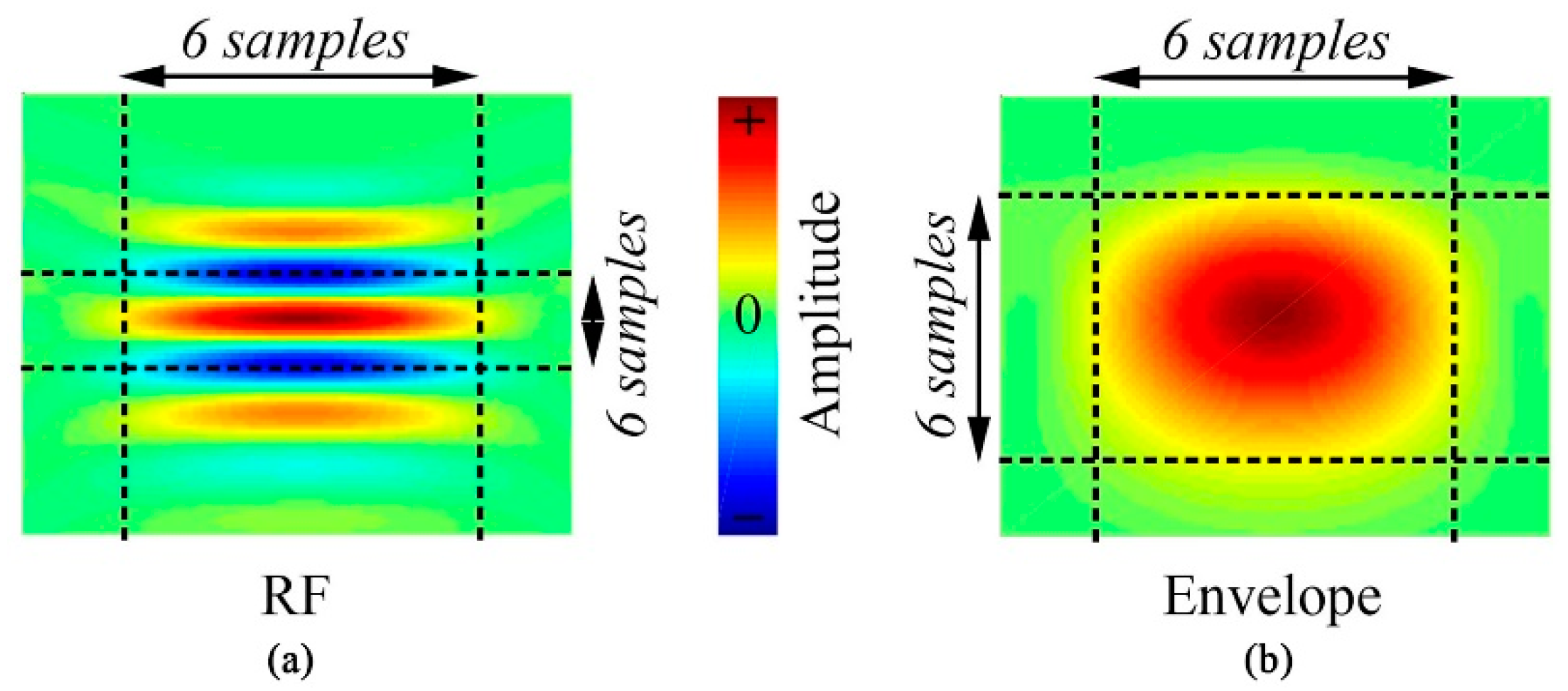
Circular-shaped CCF peaks were realized by choosing the data sampling grid such that a single period of the system’s PSF contained an equal amount of sampling points in axial and lateral direction. Firstly, concerning the RF data (Figure 1a), six samples per wavelength were beamformed in axial direction, in accordance with the all-positive-samples condition [34], resulting in an axial sampling distance of dax,rf = c/(2 × fc × 6), with c the speed of sound and fc the center frequency of the emitted waveform. The lateral sampling distance was determined according to dlat,rf = dax,rf × PSFratio × Ncycles, with PSFratio the average ratio between the lateral and axial PSF dimensions and Ncycles the number of cycles present in the PSF axially. The envelope data sampling grid (Figure 1b) was generated by down sampling the RF sampling grid in axial direction with the factor Ncycles, resulting in an axial spacing of dax,env = dax,rf × Ncycles. The lateral spacing for the envelope data was set similar to the lateral spacing of the RF data (dlat,env = dlat,rf). With these spacing settings, the peak of the CCF will appear circular-shaped when using both envelope and RF data in the multi-step ST algorithm.
2.2. Imaging Setup
An L5-12 ATL (ATL, Bothell, WA, USA), 38 mm linear array transducer was used in this work. Zero-degree plane waves were transmitted by simultaneously activating 128 elements at the center of the transducer, using a rectangular apodization window. The same 128 elements were also active in receive. The transducer parameters are listed in Table 1. The Field II ultrasound simulation program [47,48] was used for simulations and the Verasonics Vantage 256 experimental ultrasound system (Verasonics, Kirkland, WA, USA) for the experimental measurements.
2.3. Simulations
Ultrasound RF element data of blood and tissue were simulated, which are represented by a set of random point scatterers. About 300 scatterers per mm3 where used and each physical transducer element was subdivided into 10 by 10 mathematical elements to increase computational accuracy. A sampling frequency of 180 MHz was used, the resulting RF element data were down sampled to 36 MHz to mimic experimental settings. The speed of sound was assumed to be 1540 m/s.
2.3.1. Parabolic Flow in Vessel Phantom
Parabolic flow through a rigid, straight tube with a peak velocity (vmax) of 1.5 m/s was simulated at flow angles of 75° till 105°, with steps of 3°. The vessel had a lumen diameter of 6 mm and was centered at 20 mm depth. Scatterers, representing the blood, had Gaussian distributed amplitudes (mean = 5, SD = 1). Plane wave ultrasound data were simulated for pulse repetition frequencies (PRFs) of 2.5 till 15 kHz, with steps of 2.5 kHz. Table 2 provides an overview of the simulated PRFs and resulting inter-frame displacements. For each unique combination of flow angle and PRF, a pre and post frame were simulated, where in between the scatterers were propagated according to the parabolic velocity profile. This process was repeated ten times, with random initial scatterer positions, allowing 10 independent velocity estimates. No clutter filtering or time averaging were performed. Band limited noise was added to the beamformed RF data resulting in a signal-to-noise ratio (SNR) of 12 dB.
2.3.2. Carotid Vessel Wall Displacements
Simulations of the carotid artery vessel wall were performed using deformations patterns as obtained from a patient-specific finite element model (FEM) of the carotid artery at the bifurcation [40]. A transversal image plane, containing the internal and external carotid artery, was simulated. The amplitude of the scatterers representing the carotid artery were set at two, the surrounding tissue scatterers had an amplitude of one. Specular reflections were mimicked by positioning scatterers at the lumen-vessel wall and vessel wall-surrounding tissue transitions, which enhanced the realism of the RF data. Simulations of the vessel wall were performed in early systole, where peak inter-frame displacements are present and in late diastole, where low inter-frame displacements are present. A pre and post deformation frame were simulated for each time point, using a PRF of 50 Hz and 25 Hz (see Table 2) in systole and diastole, respectively. Band limited noise was added to the beamformed RF data resulting in an SNR of 30 dB.
2.4. Rotating Disk Experiments
A rotating disk experimental setup was built, providing a range of velocities at all possible beam-to-flow angles, or, a range of inter-frame displacements at full 360° range of directions. This type of setup has been used to study the performance of velocity estimation methods [29,43].
A cylindrical homogeneous phantom was created using a 15% polyvinyl alcohol (PVA) solution [39]. The solution was poured into a cylindrical mold (Øinner = 20 mm), containing a fixating-structure (see Figure 2) to attach the phantom onto the motor unit during the experiments, and subjected to three freeze-thaw cycles. Shrinkage of the phantom was present during assemblage, resulting in a final diameter of 18.2 mm. The phantom was attached to a motor unit (Closed Loop Step Motor, ARM69AC, Oriental Motor USA Corp., Torrance, CA, USA) and placed in a water tank (see Figure 2). It was rotated at a constant angular velocity, resulting in a maximum velocity at the outer edge of 18.2 cm/s. The phantom was positioned perpendicular to the transducer’s scan plane at a depth of 3.4 cm. Plane wave data were acquired continuously using a PRF of 8 kHz for 4 s.
Two different approaches were used for processing the acquired data. One approach resembling flow velocity estimation and the second approach analogous to the processing performed for the vessel wall displacement simulations.
2.4.1. Rotational Flow
After RF data beamforming and prior to velocity estimation, clutter filtering was performed. Although the phantom does not contain actual blood or tissue, including clutter filtering will give a more realistic picture of the performance of the methods for velocity estimation. A finite impulse response (FIR) filter with an order of 46 was used in combination with a temporal sliding window, not sacrificing frames for filter initialization. The −3 dB velocity cut-off point was equal to 0.068 times the Nyquist velocity. By down sampling the beamformed RF data in temporal direction, a range of PRFs (8, 4, 2 and 1 kHz) was studied. The resulting inter-frame displacements are summarized in Table 2. The same filter characteristics were used for all PRFs and estimated velocities were median averaged over 40 temporal frames.
2.4.2. Rotational Vessel Wall Displacement
Inter-frame displacements were estimated after RF data beamforming. Both PRFs of 8 and 4 kHz were studied, resembling inter-frame displacements present in early systole and late diastole of the vessel wall dynamics (see Table 2).
2.5. Beamforming Setup and Grid Definition
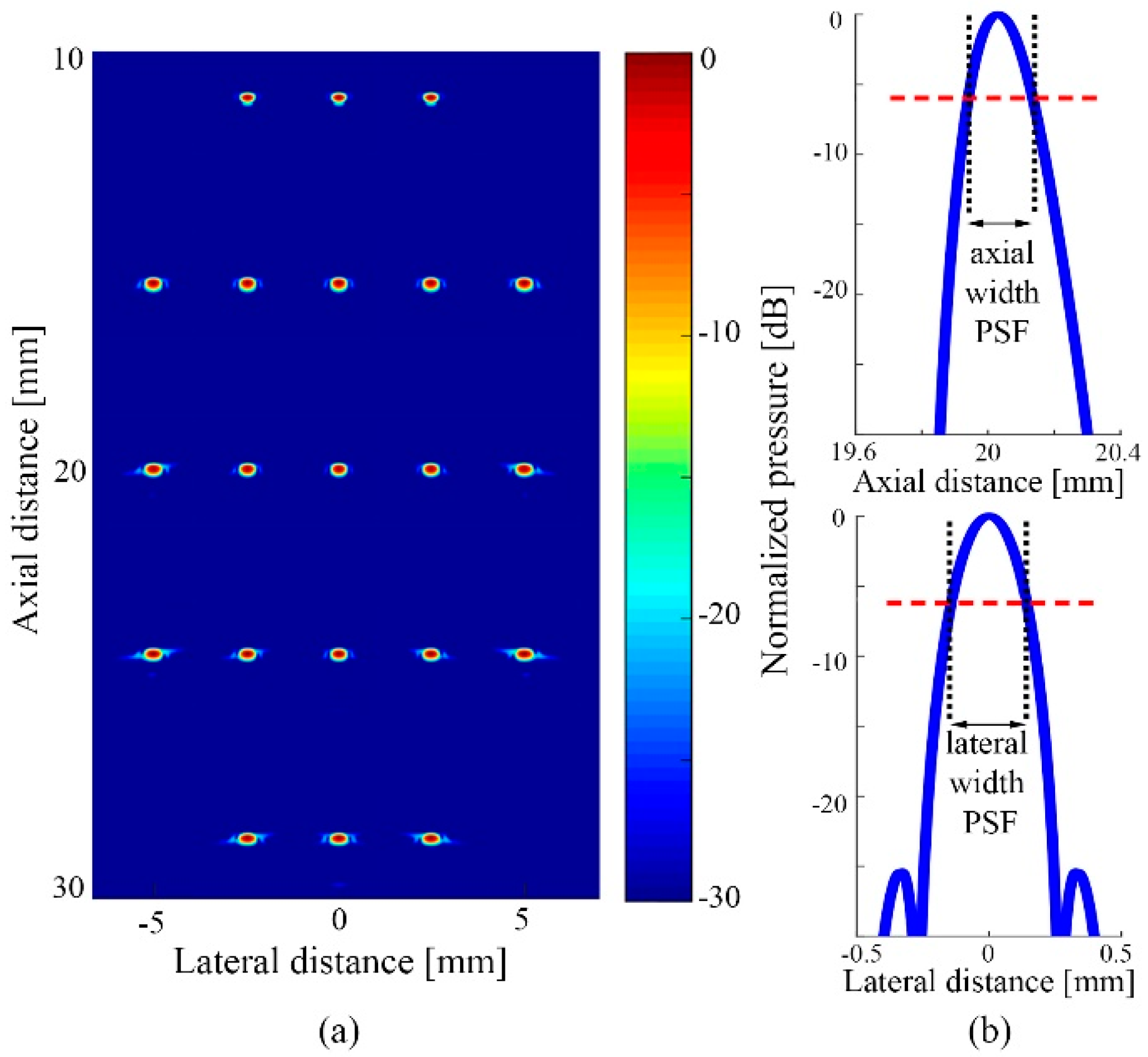
To be able to calculate the spacing for the PSF-shape-based beamforming grid, the PSF dimensions were determined for both the simulation and experimental setup (see Table 3). Field II was used to simulate the response of multiple point scatterers placed at spatial positions relevant for carotid artery imaging (Figure 3a). Simulated element data were beamformed on a high resolution grid and intensity curves for each individual scatterer were generated (Figure 3b). The axial (PSFax) and lateral (PSFlat) size of the PSFs were determined based on the −6 dB values. The PSFratio was determined according to PSFratio = PSFlat/PSFax. The resulting ratios were averaged for all simulated scatterers. The PSF dimensions were determined experimentally using a wire phantom (60 μm diameter) placed in a water tank. Plane wave data were acquired of the wire phantom and similar processing was performed to determine the PSFratio.
Delay-and-sum beamforming was used to generate RF data for every plane wave transmission at pre-specified data sampling points [39]. The data were beamformed on the PSF-shape-based grid using the axial and lateral sampling distance as specified (Section 2.1.2) for the RF data (dax,RF and dlat,RF). Consequently, the envelope data were obtained by demodulation and down sampling of the RF data in the axial direction. Furthermore, the element data were also beamformed on a conventionally spaced grid, with a lateral sampling distance equal to the pitch and 4 samples per wavelength in axial direction. Details on the grid spacing and beamforming parameters can be found in Table 3.
2.6. Multi-Step Speckle Tracking Settings
Inter-frame displacements were estimated using data beamformed on both the conventional grid and the PSF-shape-based grid. The size of the search windows was tuned to the maximum displacement expected in each situation. Spatial smoothing of the estimated displacements was performed using median filters. Inter-frame displacement estimates were multiplied by frame rate to calculate velocities.
Subsample resolution was resolved by interpolation of the CCF in both steps of the algorithm. Two types of interpolation were used: 1D parabolic fitting in each direction of the CCF independently, since it is one of the most often used interpolators in ultrasound applications as described in the Introduction, and 2D cubic interpolation, where a joint estimation of subsample displacement in both directions was obtained. The parabolic fitting is solved analytically using the commonly applied three-point parabola fitting [25,33]. 2D cubic interpolation was performed with a resulting effective upsampling factor of 10 and 1000 in the first and second step of the algorithm, respectively. For the second step, a fast in-house built implementation was used, where the high final resolution was reached iteratively by zooming in onto the peak of the CCF in multiple iteration steps. Given the CCF with its maximum at position (i,j), the new sampling points (ix,iy) are defined by ix = ixm*5iter + i and iy = iym*5iter + j, with matrices ixm and iym representing the direct neighbors of (i,j) according to ixm = [−1 0 1;−1 0 1;−1 0 1] and iym = [−1 −1 −1; 0 0 0; 1 1 1]. Ten iteration steps (iter = 1–10) were used, resulting in the effective upsampling factor of 1000. A complete overview of the settings used in the ST algorithm can be found in Table 4.
Summarized, four different combinations of beamforming grid and CCF interpolation type were studied in this work: (1) data beamformed on the conventional grid combined with 1D parabolic interpolation (conv_1Dpar) and (2) combined with 2D cubic interpolation (conv_2Dcub), (3) data beamformed on the PSF-shape-based grid combined with 1D parabolic interpolation (PSF_1Dpar) and (4) combined with 2D cubic interpolation (PSF_2Dcub).
The performance of the four approaches was studied in terms of the accuracy and precision of the velocity magnitude, velocity angle and the displacement estimates. The accuracy of the velocity magnitude and the inter-frame displacement estimates was assessed by calculating the absolute error percentage between the mean estimates and the ground truth as follows:
with i all estimated samples within the region-of-interest (ROI), ESTmean the mean of the estimates and GT the ground truth value. ESTmean was based on n = 10 realizations for the simulated parabolic flow, n = 100 ensemble averaged velocity estimates for the experimental rotational flow, and n = 100 inter-frame displacement estimates for the rotational displacement experiments. The error for the velocity angle estimates was calculated as the absolute error, i.e., error (i) =|ESTmean(i) − GT(i)|.
The precision for the velocity magnitude and inter-frame displacement estimates was assessed by calculating the relative standard deviation:
with σEST the standard deviation of the same n estimates, and GTmax the maximal ground truth value. The precision of the velocity angle estimates was calculated as the standard deviation (σEST). For the analysis of the experiments, the center of the disk (r < 1 mm) was excluded from the calculations to avoid velocities or displacements close to zero.
The performance for all methods for the vessel wall simulation was quantified by calculating the root-mean-squared error (RMSE) between estimated and ground truth axial and lateral displacements:
with N the number of estimated samples within the ROI, EST(i) the estimated value for sample i, and GT(i) the ground truth value for sample i.
3. Results
3.1. Simulations
3.1.1. Parabolic Flow in Vessel Phantom
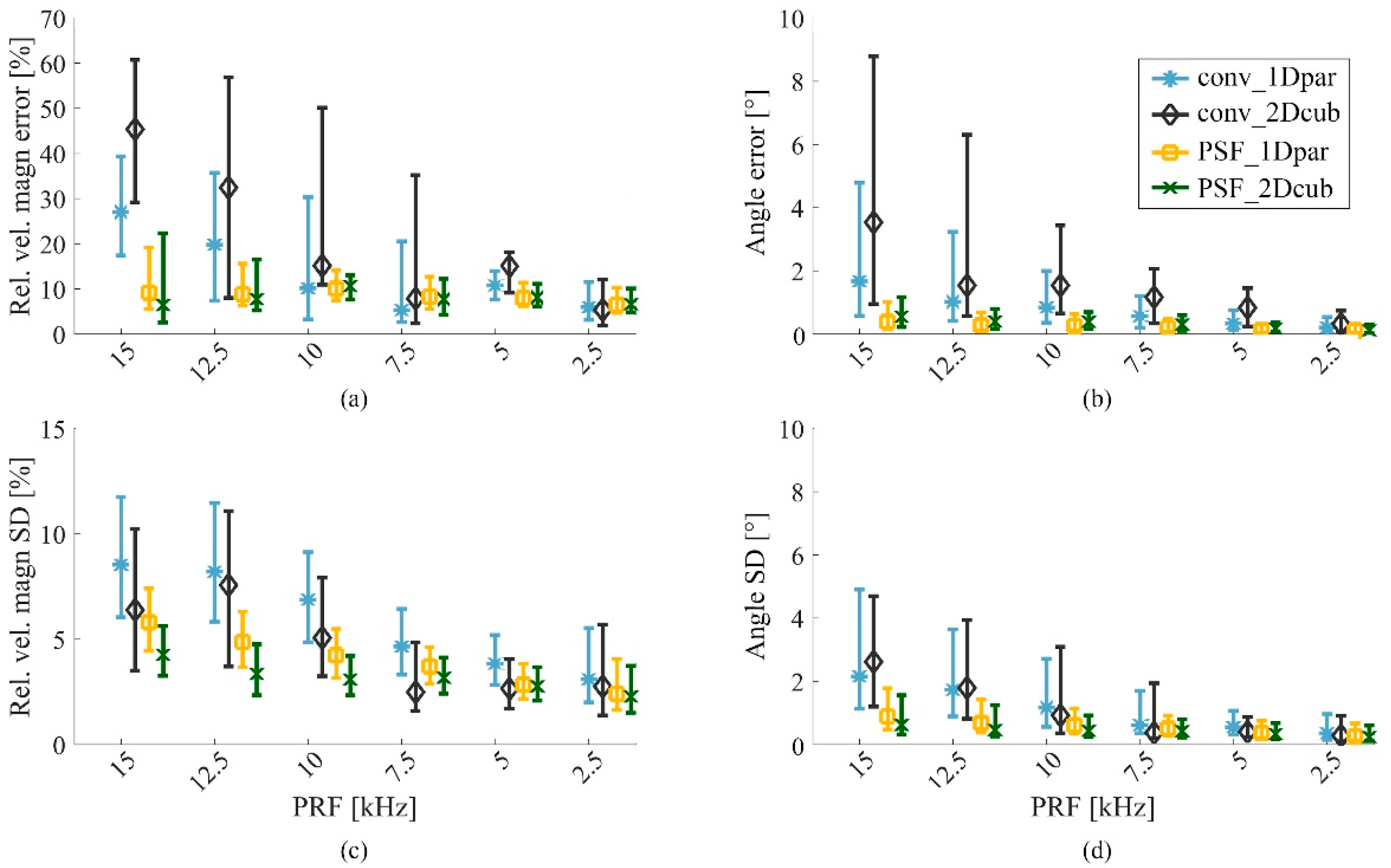
In Figure 4, the absolute bias and SD values are visualized as a function of the PRF for the parabolic flow simulations. The statistics were calculated while taking into account all simulated beam-to-flow angles. When the PRF increases, i.e., when the inter-frame displacements become smaller (see Table 2), the bias and SD for both the magnitude and angle increase. This effect is most dominant for the conventional grid, while the PSF-shape-based grid shows a more stable performance over the PRF range. Both PSF_1Dpar and PSF_2Dcub show high accuracy and precision, i.e., low bias and SD values, for the entire range of PRFs. For both methods, the median magnitude bias is below 10% and the angle bias remains below 0.55°.
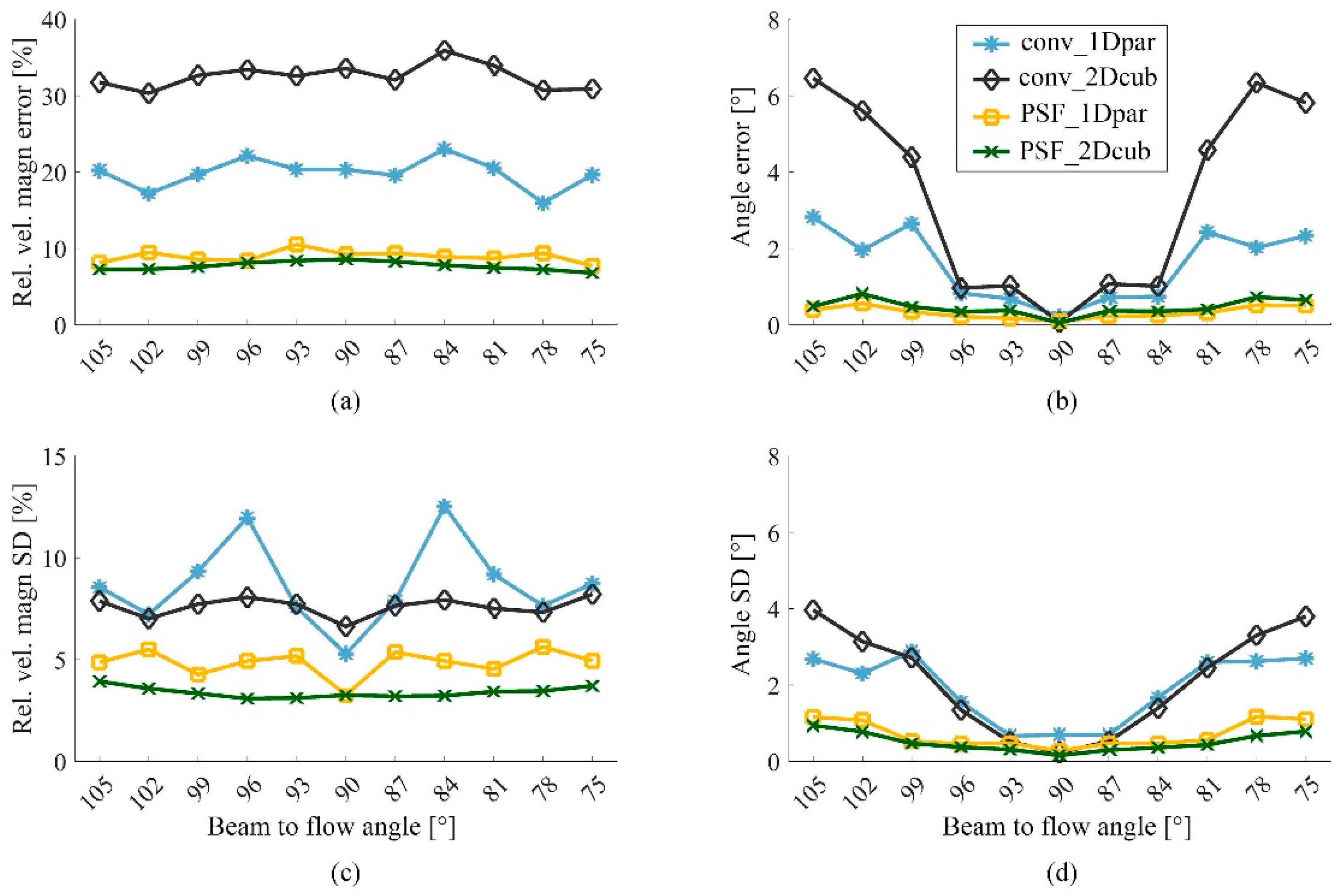
Figure 5 visualizes the dependency of the performance of the methods on beam-to-flow angle. The results were obtained using a PRF of 12.5 kHz. The accuracy and precision of the velocity angle estimates show a dependency on the beam-to-flow angle, whereas the magnitude estimate is less influenced by this. When the velocity field contains larger axial velocity components, i.e., for beam-to-flow angles different from 90°, the angle bias and SD values increase, especially for conv_1Dpar and conv_2Dcub. The PSF-shape-based grid combined with either 1D parabolic or 2D cubic interpolation shows a stable performance over the range of angles, with almost no increase of angle error and SD for angles other than 90°.
Figure 4 and Figure 5 show a competitive performance for PSF_1Dpar and PSF_2Dcub. Both methods show a stable performance for all PRFs, i.e., for 0 to 600 µm inter-frame displacements (see Table 2), and for all beam-to-flow angles. However, significantly lower median SD values for both velocity magnitude and angle can be appreciated for the PSF_2Dcub method (Wilcoxon signed-rank, p < 0.05). The median magnitude SD is at maximum 5.8% for PSF_1Dpar and 4.2% for PSF_2Dcub. Furthermore, the median angle SD is maximally 0.9° and 0.6° for PSF_1Dpar and PSF_2Dcub, respectively.
3.1.2. Carotid Vessel Wall Displacements
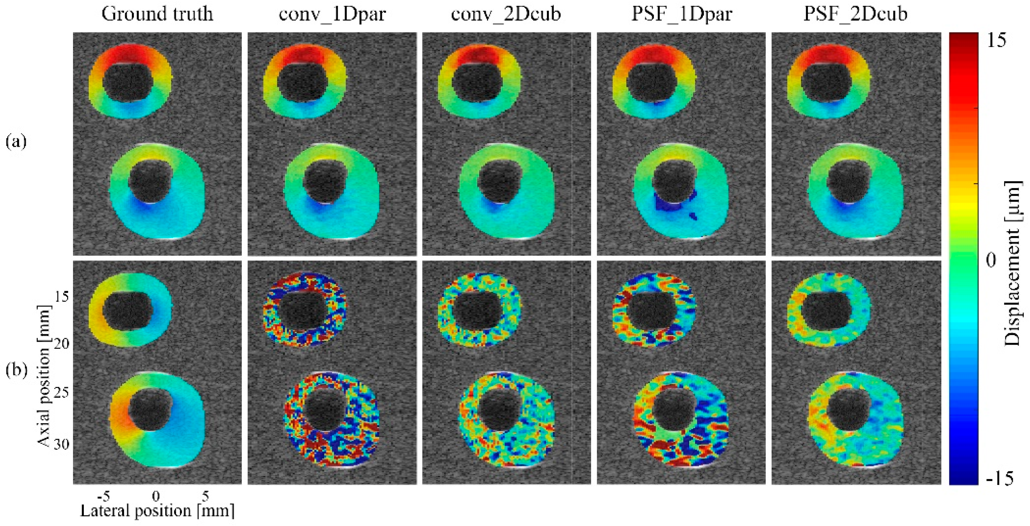
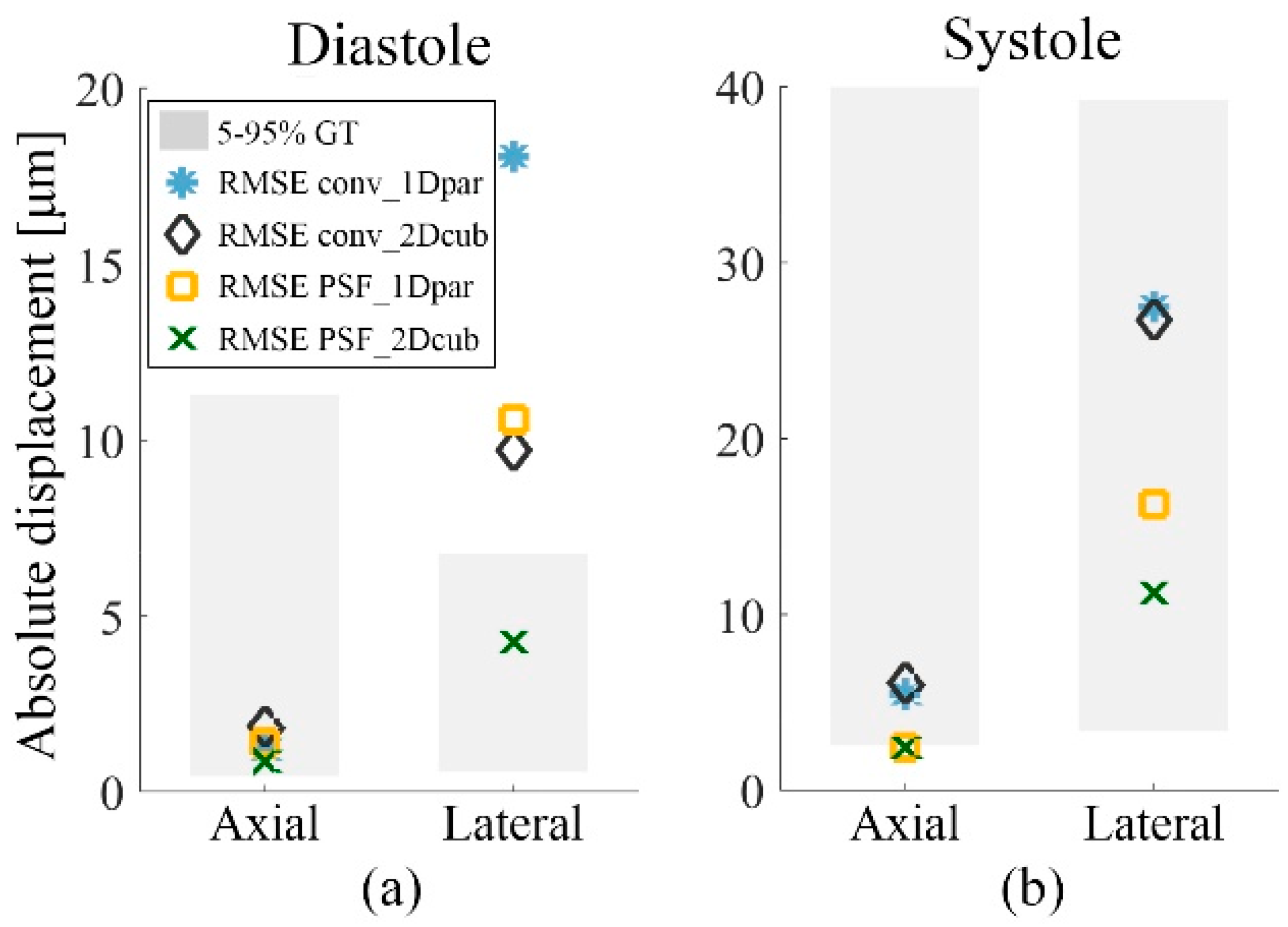
Figure 6 visualizes the estimated inter-frame displacements in the external and internal carotid vessel wall using the four different methods. Major performance difference can be seen for the lateral displacement estimation, with PSF_2Dcub showing the highest similarity with the ground truth. The RMSE values are visualized in Figure 7. The accuracy of the displacement estimates in the axial direction is higher than in the lateral direction, showing lower RMSE values for all four methods. This can also be appreciated from Figure 6. The largest performance differences between the four methods are observed for the lateral estimates. The PSF_2Dcub method shows lowest RMSEs for both the diastolic and systolic phase.
3.2. Rotating Disk Experiments
3.2.1. Rotational Flow
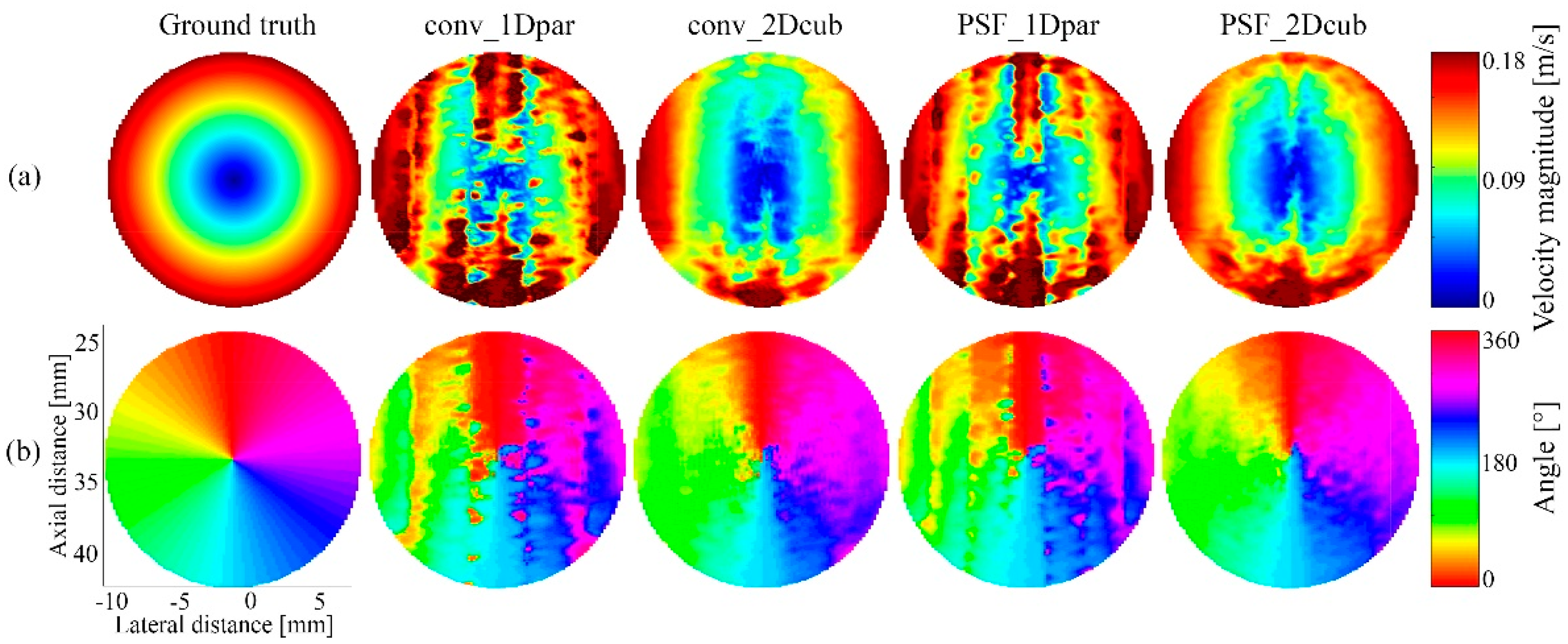
Figure 8 shows the estimated and reference velocity magnitude and angle for the rotating disk experiment. Single ensemble-averaged velocity estimates for a PRF of 4 kHz are shown. Highest resemblance between velocity magnitude and ground truth is found for the PSF_2Dcub method. Here, largest deviations from the ground truth are observed in the center vertical slice of the disk, where velocities are mainly in lateral direction. This is a combined effect of the lower lateral resolution and clutter filtering. Due to the smaller axial velocity component in these regions, the estimates will be more influenced by the clutter filter [49,50]. In the bottom row of Figure 8, the angle estimation performance is visualized. Both the conv_2Dcub and PSF_2Dcub methods show good resemblance with the ground truth velocity angle.
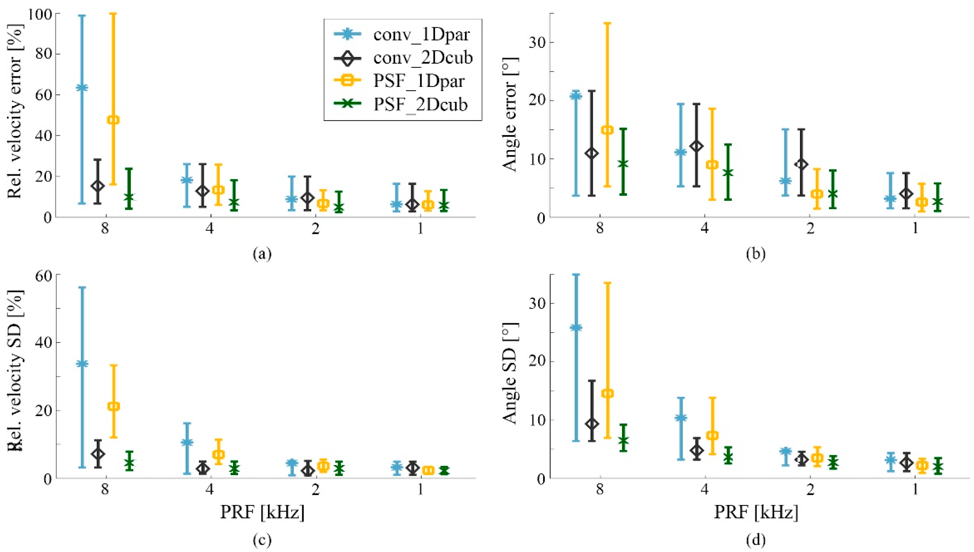
In Figure 9, the absolute bias and SD values are visualized as a function of the PRF. Similar effects can be seen as in the parabolic flow simulations: when inter-frame displacements become smaller, the bias and SD for both velocity magnitude and angle increase. This is most profound for the conv_1Dpar and PSF_1Dpar methods. The conv_2Dcub method shows a stable performance over the range of PRFs, although slightly higher bias and SD values are found as compared to the PSF_2Dcub method, especially for a PRF of 8 and 4 kHz. The PSF_2Dcub method shows a stable performance over the PRF-range, with low bias and SD values. Even for very small inter-frame displacements, the accuracy and precision of this method are excellent. A median velocity magnitude bias of maximally 10% and a median angle bias of 9.2° are found. The median SD for the velocity magnitude and angle are maximally 4.6% and 6.5°, respectively.
3.2.2. Rotational Vessel Wall Displacements
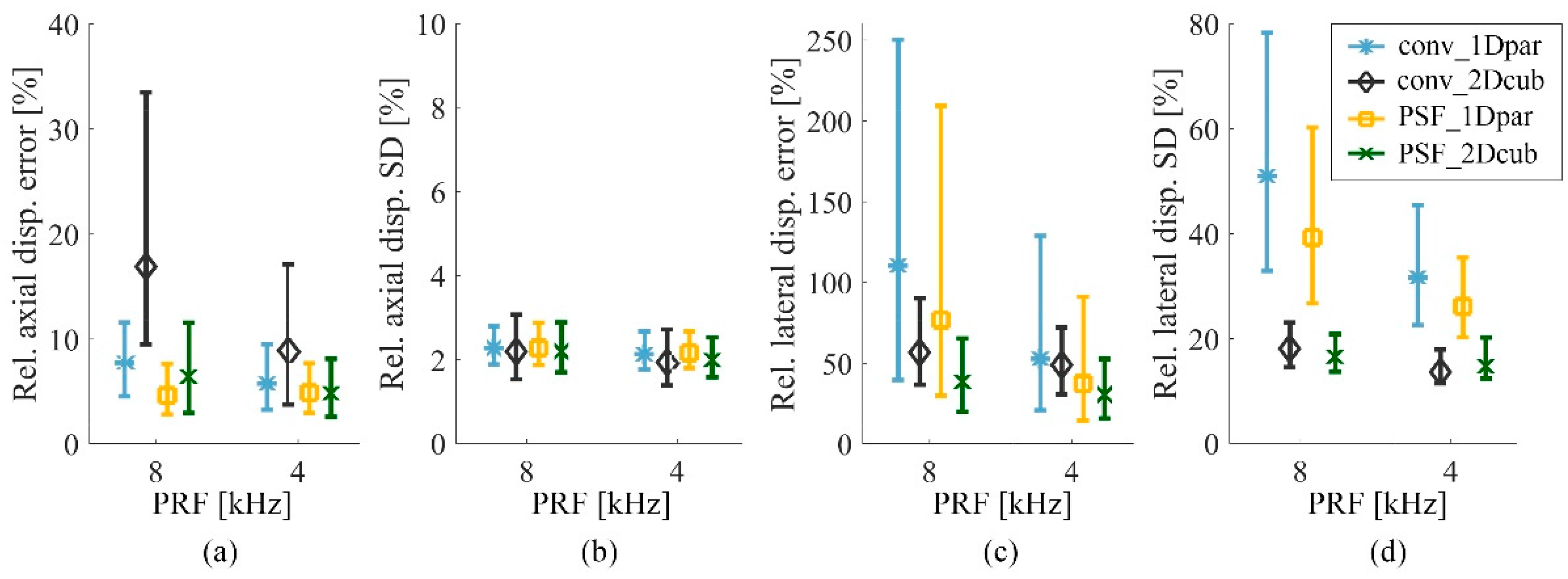
In Figure 10, results for the rotating disk experiments are visualized when processed as vessel wall. Similar as in the vessel wall simulation study, the performance of the four methods is comparable for the axial displacement estimation. Furthermore, the axial accuracy is higher as the lateral displacement estimation accuracy. The lowest median lateral displacement error can be appreciated for the PSF_2Dcub method, although interquartile ranges of all methods show overlap. Furthermore, the precision of the lateral displacement estimation is highest for the PSF_2Dcub and conv_2Dcub methods. Overall, the PSF_2Dcub method shows the most stable performance with respect to the PRFs.
4. Discussion
In this paper, a new method has been proposed to determine the beamforming grid for ultrafast data based on the dimensions of the imaging system’s PSF. As a result of this data sampling, the CCFs used in the ST algorithm will contain circular-shaped peaks. It was hypothesized that once combined with 2D cubic interpolation, this would increase the accuracy and precision of subsample displacement estimation and thereby enlarge the range of detectable displacements and velocities. Both simulations and experiments were conducted to characterize the performance of the method. A comparison was made with conventionally spaced beamformed data and the very commonly used 1D parabolic subsample displacement estimation method. The results confirmed our hypothesis: the PSF-shape-based beamforming grid combined with 2D cubic interpolation (PSF_2Dcub) showed the most accurate and stable performance with respect to the range of inter-frame displacements, both for the assessment of blood flow and vessel wall dynamics. Besides, the performance of the method was least affected by motion direction or beam-to-flow angle.
An important finding was that largest performance differences between the four methods were found for the lateral displacement component. This can be appreciated for the vessel wall (Figure 6, Figure 7 and Figure 10), but also for the flow results (Figure 8), in the upper and lower part of the disk, where velocities are predominantly in lateral direction. Furthermore, the accuracy and precision of the axial displacement estimates is consistently higher as compared to the lateral estimates, due to the higher resolution and presence of phase information. This also explains why the performance difference is less obvious in the axial direction and very clearly visible in the lateral direction. No phase information is available and the frequency content is lower in the lateral direction. Consequently, more benefit is gained from the proposed methodology.
Several functions can be used to interpolate the CCF for subsample displacement estimation. In this work, we used 1D parabolic interpolation, one of the most widely used functions, to compare to our proposed methodology. The results however, show that 1D parabolic is less optimal for subsample displacement estimation. Large bias, SD and RMSE values were found when 1D parabolic interpolation was used for CCF interpolation. More specifically, large bias and SD values on the lateral axis were shown when subsample displacements existed on the axial axis. This effect can be appreciated in Figure 8, where vertically stripped patterns are visible in the magnitude and angle estimates for the PSF_1Dpar en conv_1Dpar methods. These patterns originate from the inaccurate lateral displacement estimates in regions of subsample axial displacements, as also reported earlier [33]. The benefit of using 1D parabolic interpolation is the low computational cost, whereas 2D cubic interpolation increases computational time. Therefore, the trade-off between computational time and performance needs to be considered.
One limitation of this study is that a single 2D interpolator was investigated. Many other studies have investigated the use of other shapes and functions, such as cosine, parabolic or spline [25,33,35,51,52], most often in 1D. However, none of these interpolators have been studied before in the context of the proposed methodology, i.e., in combination with the freedom of choosing the beamforming grid and thereby influencing the CCF shape. Further investigation should be performed to compare different 2D interpolators in combination with the PSF-shape-based grid. 2D fitting of the CCF peak instead of interpolation is not considered in this work, due to the enormous increase of computational time, which makes its use less practical.
Another method to improve subsample displacement estimation is by interpolation of the echo signal. This method was often used in combination with conventionally acquired data and reduced the error by the up sample factor. However, the computational cost increased significantly [25,53]. The benefit of the use of ultrafast data is that instead of interpolating the echo signals, actual focusing of the signals can be performed in receive, as a post-processing step. This work shows that no excessive sampling of the RF data is required when using knowledge of the PSF dimensions to beamform the data combined with a suitable 2D subsample interpolation method.
The proposed methodology is based upon the statement that the CCF shape is primarily determined by the shape of the PSF. While it is one of the most important factors influencing the appearance of the CCF, it is known that other factors will also be of influence. In general, the performance of motion estimation methods will degrade as a result of signal decorrelation. Factors such as out-of-plane motion, presence of strong gradients within the displacement field and large deformations can hamper the match of the signal template within the search window, thereby influencing the appearance of the CCF. Smartly choosing data type and window sizes is recommended in those situations [25,54] and aligning and stretching methods are suggested to minimize signal decorrelation [55,56]. Although these and other factors will also influence the CCF shape, the proposed methodology was successful under the circumstances tested in this work.
To determine the spacing of the PSF-shape-based beamforming grid, a single average PSFratio was used in this work. This was allowed since for carotid artery imaging, the PSF is nearly constant within the region of interest. However, for other applications, such as cardiac imaging, the size of the PSF will change with respect to the position in the imaging plane, amongst others due to the frequency dependent attenuation and location of the echo with respect to the ultrasonic beam [34]. These effects can be seen in the work of Tong et al. [57]. However, application of the PSF-shape-based grid is still possible, when using variable grid spacing tuned to the PSF shape locally. Nillesen et al. [58] showed first results using such a multi-zone, depth-dependent PSF-shape-based grid for cardiac motion imaging. The beamforming grid resolution was adjusted to the local PSF shape. This work also shows that the proposed beamforming strategy is not limited to linear array imaging. The PSF-shape-based beamforming grid can easily be used for data obtained with different transducer types, such as a phased array. The only requirement for using this method is the characterization of the imaging system by determining the (local) dimensions of the PSF.
In this work, the dimensions of the PSFs were determined using the response of single scatterers. When processing data acquired in vivo, a more sophistic approach could be favorable, which includes other factors influencing the shape of the PSF, such as attenuation. A representative estimate of the PSFratio could be obtained by using the spatial auto covariance method [59] to determine the speckle size in a B-mode image. Since speckle size is proportional to the dimensions of the PSF [60,61], this will provide the required information to determine the PSF-shape based beamforming grid.
In the present work, a large range of inter-frame displacements were studied by imaging with different PRFs. A stable and accurate performance of the proposed method was shown with respect to this large range of displacements. This shows the applicability of the proposed methodology for a broad field of research: it allows to study the dynamic behavior of multiple tissue types, such as the carotid artery, the heart and breast tissue, where very small displacements need to be captured, but also very large displacements and deformations can be present simultaneously.
In this work, the proposed beamforming strategy was combined with cross-correlation-based ST. However, this strategy is also applicable to other pattern matching functions, for example the sum of absolute squared differences. Furthermore, while this work presents a methodology in 2D, it could be easily adapted to 3D. The system’s PSF needs to be characterized in 3 dimensions and interpolation of the 3D CCF in 3 directions should be performed simultaneously.
Zero-degree plane waves were used to acquire data in this work. The estimation of vessel wall displacements and blood flow velocities could be further improved by performing displacement compounding [40,49,62], a method introduced by Techavipoo et al. [63] and adapted for vascular strain estimation [64] and blood flow imaging [52]. Angled plane waves are used to derive the displacement or velocity vector, using solely axial displacement estimates. However, to improve the accuracy and precision of the estimates, often 2D ST is performed to acquire these axial displacements [62,64,65], meaning the accuracy of both the lateral and axial displacement estimates influence the performance of the compounding method. Therefore, displacement compounding would also strongly benefit from the methodology as presented in this work.
5. Conclusions
In this paper, a framework for robust displacement estimation in ultrafast ultrasound data was presented. It can be used as a protocolled way to beamform ultrafast data and obtain accurate estimates of the tissue displacements. The success of this new methodology is based on the following important concepts: the matching shape of the CCF peak and the interpolation function, the equal number of sample points in axial and lateral direction throughout the peak, and the use of 2D instead of 1D interpolation functions to acquire joint estimation of subsample displacements in both directions. The proposed method defines the beamforming grid based on the system’s PSF to generate standardized circular-shaped CCFs which match with a 2D cubic interpolation function. The results presented in this work confirm the hypothesis; increased accuracy and precision were found for 2D motion estimation using the PSF-shape-based beamforming grid combined with 2D cubic subsample interpolation of the CCF. This was shown for a wide range of displacements or velocities present in carotid vessel wall and blood flow dynamics.
Acknowledgments
This research is supported by the Dutch Technology Foundation STW (NKG 12122), which is part of the Netherlands Organization for Scientific Research (NWO), and which is partly funded by the Ministry of Economic Affairs. The authors want to gratefully acknowledge the support of A. Nikolaev, MSc for his assistance in the rotating disk experiments.
Author Contributions
Anne E. C. M. Saris, Stein Fekkes, Maartje M. Nillesen, Hendrik H. G. Hansen and Chris L. de Korte conceived and designed the experiments/simulations; Anne E. C. M. Saris performed the simulations with support of Stein Fekkes, Anne E. C. M. Saris performed the experiments; Anne E. C. M. Saris analyzed the data with support of Stein Fekkes, Maartje M. Nillesen, Hendrik H. G. Hansen and Chris L. de Korte; Anne E. C. M. Saris is the main author of the paper; critical revisions were provided by all co-authors.
Conflicts of Interest
The authors declare no conflicts of interest.
References
- Evans, D.H.; Jensen, J.A.; Nielsen, M.B. Ultrasonic colour doppler imaging. Interface Focus 2011, 1, 490–502. [Google Scholar] [CrossRef] [PubMed] [Green Version]
- D’Hooge, J.; Heimdal, A.; Jamal, F.; Kukulski, T.; Bijnens, B.; Rademakers, F.; Hatle, L.; Suetens, P.; Sutherland, G.R. Regional strain and strain rate measurements by cardiac ultrasound: Principles, implementation and limitations. Eur. J. Echocardiogr. 2000, 1, 154–170. [Google Scholar] [CrossRef] [PubMed]
- Konofagou, E.E.; D’Hooge, J.; Ophir, J. Myocardial elastography—A feasibility study in vivo. Ultrasound Med. Biol. 2002, 28, 475–482. [Google Scholar] [CrossRef]
- De Korte, C.L.; Pasterkamp, G.; van der Steen, A.F.W.; Woutman, H.A.; Bom, N. Characterization of plaque components using intravascular ultrasound elastography in human femoral and coronary arteries in vitro. Circulation 2000, 102, 617–623. [Google Scholar] [CrossRef] [PubMed]
- Krouskop, T.A.; Wheeler, T.M.; Kallel, F.; Garra, B.S.; Hall, T. Elastic moduli of breast and prostate tissues under compression. Ultrason. Imaging 1998, 20, 260–274. [Google Scholar] [CrossRef] [PubMed]
- Blessberger, H.; Binder, T. Non-invasive imaging: Two dimensional speckle tracking echocardiography: Basic principles. Heart 2010, 96, 716–722. [Google Scholar] [CrossRef] [PubMed]
- Grubb, N.R.; Fleming, A.; Sutherland, G.R.; Fox, K.A. Skeletal muscle contraction in healthy volunteers: Assessment with doppler tissue imaging. Radiology 1995, 194, 837–842. [Google Scholar] [CrossRef] [PubMed]
- Luo, J.; Li, R.X.; Konofagou, E.E. Pulse wave imaging of the human carotid artery: An in vivo feasibility study. IEEE Trans. Ultrason. Ferroelectr. Freq. Control 2012, 59, 174–181. [Google Scholar] [CrossRef] [PubMed]
- Papadacci, C.; Pernot, M.; Couade, M.; Fink, M.; Tanter, M. High-contrast ultrafast imaging of the heart. IEEE Trans. Ultrason. Ferroelectr. Freq. Control 2014, 61, 288–301. [Google Scholar] [CrossRef] [PubMed]
- Tanter, M.; Bercoff, J.; Sandrin, L.; Fink, M. Ultrafast compound imaging for 2-d motion vector estimation: Application to transient elastography. IEEE Trans. Ultrason. Ferroelectr. Freq. Control 2002, 49, 1363–1374. [Google Scholar] [CrossRef] [PubMed]
- Ricci, P.; Maggini, E.; Mancuso, E.; Lodise, P.; Cantisani, V.; Catalano, C. Clinical application of breast elastography: State of the art. Eur. J. Radiol. 2014, 83, 429–437. [Google Scholar] [CrossRef] [PubMed]
- Sadigh, G.; Carlos, R.C.; Neal, C.H.; Dwamena, B.A. Accuracy of quantitative ultrasound elastography for differentiation of malignant and benign breast abnormalities: A meta-analysis. Breast Cancer Res. Treat. 2012, 134, 923–931. [Google Scholar] [CrossRef] [PubMed]
- Gamble, G.; Zorn, J.; Sanders, G.; MacMahon, S.; Sharpe, N. Estimation of arterial stiffness, compliance, and distensibility from m-mode ultrasound measurements of the common carotid artery. Stroke 1994, 25, 11–16. [Google Scholar] [CrossRef] [PubMed]
- Schaar, J.A.; de Korte, C.L.; Mastik, F.; Strijder, C.; Pasterkamp, G.; Serruys, P.W.; van der Steen, A.F.W. Characterizing vulnerable plaque features by intravascular elastography. Circulation 2003, 108, 2636–2641. [Google Scholar] [CrossRef] [PubMed]
- Hansen, H.H.; de Borst, G.J.; Bots, M.L.; Moll, F.L.; Pasterkamp, G.; de Korte, C.L. Compound ultrasound strain imaging for noninvasive detection of (fibro)atheromatous plaques: Histopathological validation in human carotid arteries. JACC Cardiovasc. Imaging 2016, 9, 1466–1467. [Google Scholar] [CrossRef] [PubMed]
- Hansen, H.H.; de Borst, G.J.; Bots, M.L.; Moll, F.L.; Pasterkamp, G.; de Korte, C.L. Validation of noninvasive in vivo compound ultrasound strain imaging using histologic plaque vulnerability features. Stroke 2016, 47, 2770–2775. [Google Scholar] [CrossRef] [PubMed]
- Klingelhofer, J. Ultrasonography of carotid stenosis. Cerebrovasc. Dis. 2013, 35, 1. [Google Scholar] [CrossRef]
- Greene, E.R.; Eldridge, M.W.; Voyles, W.F.; Miranda, F.G.; Davis, J.G. Quantitative evaluation of atherosclerosis using doppler ultrasound. IEEE Trans. Med. Imaging 1982, 1, 68–78. [Google Scholar] [CrossRef] [PubMed]
- Van der Worp, H.B.; Bonati, L.H.; Brown, M.M. Carotid stenosis. N. Engl. J. Med. 2013, 369, 2359. [Google Scholar] [PubMed]
- Leitman, M.; Lysyansky, P.; Sidenko, S.; Shir, V.; Peleg, E.; Binenbaum, M.; Kaluski, E.; Krakover, R.; Vered, Z. Two-dimensional strain-a novel software for real-time quantitative echocardiographic assessment of myocardial function. J. Am. Soc. Echocardiogr. 2004, 17, 1021–1029. [Google Scholar] [CrossRef] [PubMed]
- Trahey, G.E.; Allison, J.W.; von Ramm, O.T. Angle independent ultrasonic detection of blood flow. IEEE Trans. Biomed. Eng. 1987, 34, 965–967. [Google Scholar] [CrossRef] [PubMed]
- Bohs, L.N.; Trahey, G.E. A novel method for angle independent ultrasonic imaging of blood flow and tissue motion. IEEE Trans. Biomed. Eng. 1991, 38, 280–286. [Google Scholar] [CrossRef] [PubMed]
- Ophir, J.; Céspedes, I.; Ponnekanti, H.; Yazdi, Y.; Li, X. Elastography: A quantitative method for imaging the elasticity of biological tissues. Ultrason. Imaging 1991, 13, 111–134. [Google Scholar] [CrossRef] [PubMed]
- Bohs, L.N.; Geiman, B.J.; Anderson, M.E.; Breit, S.M.; Trahey, G.E. Ensemble tracking for 2d vector velocity measurement: Experimental and initial clinical results. IEEE Trans. Ultrason. Ferroelectr. Freq. Control 1998, 45, 912–924. [Google Scholar] [CrossRef] [PubMed]
- Lopata, R.G.; Nillesen, M.M.; Hansen, H.H.G.; Gerrits, I.H.; Thijssen, J.M.; de Korte, C.L. Performance evaluation of methods for two-dimensional displacement and strain estimation using ultrasound radio frequency data. Ultrasound Med. Biol. 2009, 35, 796–812. [Google Scholar] [CrossRef] [PubMed]
- Bohs, L.N.; Geiman, B.J.; Anderson, M.E.; Gebhart, S.C.; Trahey, G.E. Speckle tracking for multi-dimensional flow estimation. Ultrasonics 2000, 38, 369–375. [Google Scholar] [CrossRef]
- Shattuck, D.P.; Weinshenker, M.D.; Smith, S.W.; von Ramm, O.T. Explososcan: A parallel processing technique for high speed ultrasound imaging with linear phased arrays. J. Acoust. Soc. Am. 1984, 75, 1273–1282. [Google Scholar] [CrossRef] [PubMed]
- Fadnes, S.; Nyrnes, S.A.; Torp, H.; Lovstakken, L. Shunt flow evaluation in congenital heart disease based on two-dimensional speckle tracking. Ultrasound Med. Biol. 2014, 40, 2379–2391. [Google Scholar] [CrossRef] [PubMed]
- Fadnes, S.; Ekroll, I.K.; Nyrnes, S.A.; Torp, H.; Lovstakken, L. Robust angle-independent blood velocity estimation based on dual-angle plane wave imaging. IEEE Trans. Ultrason. Ferroelectr. Freq. Control 2015, 62, 1757–1767. [Google Scholar] [CrossRef] [PubMed]
- Udesen, J.; Gran, F.; Hansen, K.L.; Jensen, J.A.; Thomsen, C.; Nielsen, M.B. High frame-rate blood vector velocity imaging using plane waves: Simulations and preliminary experiments. IEEE Trans. Ultrason. Ferroelectr. Freq. Control 2008, 55, 1729–1743. [Google Scholar] [CrossRef] [PubMed]
- Jensen, J.A.; Nikolov, S.I.; Udesen, J.; Munk, P.; Hansen, K.L.; Pedersen, M.M.; Hansen, P.M.; Nielsen, M.B.; Oddershede, N.; Kortbek, J.; et al. Recent advances in blood flow vector velocity imaging. In Proceedings of the 2011 IEEE International, Ultrasonics Symposium (IUS), Orlando, FL, USA, 18–21 October 2011; pp. 262–271. [Google Scholar]
- Swillens, A.; Segers, P.; Torp, H.; Lovstakken, L. Two-dimensional blood velocity estimation with ultrasound: Speckle tracking versus crossed-beam vector doppler based on flow simulations in a carotid bifurcation model. IEEE Trans. Ultrason. Ferroelectr. Freq. Control 2010, 57, 327–339. [Google Scholar] [CrossRef] [PubMed]
- Zahiri Azar, R.; Goksel, O.; Salcudean, S.E. Sub-sample displacement estimation from digitized ultrasound rf signals using multi-dimensional polynomial fitting of the cross-correlation function. IEEE Trans. Ultrason. Ferroelectr. Freq. Control 2010, 57, 2403–2420. [Google Scholar] [CrossRef] [PubMed]
- Céspedes, E.I.; Huang, Y.; Ophir, J.; Spratt, S. Methods for estimation of subsample time delays of digitized echo signals. Ultrason. Imaging 1995, 17, 142–171. [Google Scholar] [CrossRef] [PubMed]
- Langeland, S.; D’Hooge, J.; Torp, H.; Bijnens, B.; Suetens, P. Comparison of time-domain displacement estimators for two-dimensional rf tracking. Ultrasound Med. Biol. 2003, 29, 1177–1186. [Google Scholar] [CrossRef]
- Viola, F.; Walker, W.F. A spline-based algorithm for continuous time-delay estimation using sampled data. IEEE Trans. Ultrason. Ferroelectr. Freq. Control 2005, 52, 80–93. [Google Scholar] [CrossRef] [PubMed]
- Luo, J.; Konofagou, E.E. Effects of various parameters on lateral displacement estimation in ultrasound elastography. Ultrasound Med. Biol. 2009, 35, 1352–1366. [Google Scholar] [CrossRef] [PubMed]
- Swillens, A.; Segers, P.; Lovstakken, L. Two-dimensional flow imaging in the carotid bifurcation using a combined speckle tracking and phase-shift estimator: A study based on ultrasound simulations and in vivo analysis. Ultrasound Med. Biol. 2010, 36, 1722–1735. [Google Scholar] [CrossRef] [PubMed] [Green Version]
- Hansen, H.H.; Saris, A.E.; Vaka, N.R.; Nillesen, M.M.; de Korte, C.L. Ultrafast vascular strain compounding using plane wave transmission. J. Biomech. 2014, 47, 815–823. [Google Scholar] [CrossRef] [PubMed] [Green Version]
- Fekkes, S.; Swillens, A.E.; Hansen, H.H.; Saris, A.E.; Nillesen, M.M.; Iannaccone, F.; Segers, P.; de Korte, C.L. 2-d versus 3-d cross-correlation-based radial and circumferential strain estimation using multiplane 2-d ultrafast ultrasound in a 3-d atherosclerotic carotid artery model. IEEE Trans. Ultrason. Ferroelectr. Freq. Control 2016, 63, 1543–1553. [Google Scholar] [CrossRef] [PubMed]
- Nayak, R.; Huntzicker, S.; Ohayon, J.; Carson, N.; Dogra, V.; Schifitto, G.; Doyley, M.M. Principal strain vascular elastography: Simulation and preliminary clinical evaluation. Ultrasound Med. Biol. 2017, 43, 682–699. [Google Scholar] [CrossRef] [PubMed]
- Korukonda, S.; Nayak, R.; Carson, N.; Schifitto, G.; Dogra, V.; Doyley, M.M. Noninvasive vascular elastography using plane-wave and sparse-array imaging. IEEE Trans. Ultrason. Ferroelectr. Freq. Control 2013, 60, 332–342. [Google Scholar] [CrossRef] [PubMed]
- Villagomez Hoyos, C.A.; Stuart, M.B.; Hansen, K.L.; Nielsen, M.B.; Jensen, J.A. Accurate angle estimator for high-frame-rate 2-d vector flow imaging. IEEE Trans. Ultrason. Ferroelectr. Freq. Control 2016, 63, 842–853. [Google Scholar] [CrossRef] [PubMed]
- Saris, A.E.; Nillesen, M.M.; Fekkes, S.; Hansen, H.H.; de Korte, C.L. Robust blood velocity estimation using point-spread-function-based beamforming and multi-step speckle tracking. In Proceedings of the IEEE Ultrasonics Symposium, Taipei, Taiwan, 21–24 October 2015; pp. 1–4. [Google Scholar]
- Lopata, R.G.P.; Nillesen, M.M.; Gerrits, I.H.; Thijssen, J.M.; Kapusta, L.; de Korte, C.L. In vivo 3d cardiac and skeletal muscle strain estimation. In Proceedings of the IEEE Ultrasonics, Vancouver, BC, Canada, 2–6 October 2006; pp. 744–747. [Google Scholar]
- Shi, H.; Varghese, T. Two-dimensional multi-level strain estimation for discontinuous tissue. Phys. Med. Biol. 2007, 52, 389–401. [Google Scholar] [CrossRef] [PubMed]
- Jensen, J.A.; Svendsen, N.B. Calculation of pressure fields from arbitrarily shaped, apodized, and excited ultrasound transducers. IEEE Trans. Ultrason. Ferroelectr. Freq. Control 1992, 39, 262–267. [Google Scholar] [CrossRef] [PubMed] [Green Version]
- Jensen, J.A. Field: A program for simulating ultrasound systems. Med. Biol. Eng. Comput. 1996, 34 Pt 1, 351–353. [Google Scholar]
- Saris, A.E.; Hansen, H.H.; Fekkes, S.; Nillesen, M.M.; Rutten, M.C.; de Korte, C.L. A comparison between compounding techniques using large beam-steered plane wave imaging for blood vector velocity imaging in a carotid artery model. IEEE Trans. Ultrason. Ferroelectr. Freq. Control 2016, 63, 1758–1771. [Google Scholar] [CrossRef] [PubMed]
- Fadnes, S.; Bjaerum, S.; Torp, H.; Lovstakken, L. Clutter filtering influence on blood velocity estimation using speckle tracking. IEEE Trans. Ultrason. Ferroelectr. Freq. Control 2015, 62, 2079–2091. [Google Scholar] [CrossRef] [PubMed] [Green Version]
- Lai, X.; Torp, H. Interpolation methods for time-delay estimation using cross-correlation method for blood velocity measurement. IEEE Trans. Ultrason. Ferroelectr. Freq. Control 1999, 46, 277–290. [Google Scholar] [PubMed]
- Viola, F.; Coe, R.L.; Owen, K.; Guenther, D.A.; Walker, W.F. Multi-dimensional spline-based estimator (muse) for motion estimation: Algorithm development and initial results. Ann. Biomed. Eng. 2008, 36, 1942–1960. [Google Scholar] [CrossRef] [PubMed]
- Konofagou, E.; Ophir, J. A new elastographic method for estimation and imaging of lateral displacements, lateral strains, corrected axial strains and poisson’s ratios in tissues. Ultrasound Med. Biol. 1998, 24, 1183–1199. [Google Scholar] [CrossRef]
- Keane, R.D.; Adrian, R.J. Theory of cross-correlation analysis of piv images. Appl. Sci. Res. 1992, 49, 191–215. [Google Scholar] [CrossRef]
- Lopata, R.G.P.; Hansen, H.H.G.; Nillesen, M.M.; Thijssen, J.M.; Kapusta, L.; de Korte, C.L. Methodical study on the estimation of strain in shearing and rotating structures using radio frequency ultrasound based on 1-d and 2-d strain estimation techniques. IEEE Trans. Ultrason. Ferroelectr. Freq. Control 2010, 57, 855–865. [Google Scholar] [CrossRef] [PubMed]
- Alam, S.K.; Ophir, J. Reduction of signal decorrelation from mechanical compression of tissues by temporal stretching: Applications to elastography. Ultrasound Med. Biol. 1997, 23, 95–105. [Google Scholar] [CrossRef]
- Tong, L.; Gao, H.; Choi, H.F.; D’hooge, J. Comparison of conventional parallel beamforming with plane wave and diverging wave imaging for cardiac applications: A simulation study. IEEE Trans. Ultrason. Ferroelectr. Freq. Control 2012, 59, 1654–1663. [Google Scholar] [CrossRef] [PubMed]
- Nillesen, M.M.; Saris, A.E.C.M.; Hansen, H.H.; Fekkes, S.; van Slochteren, F.J.; Bovendeerd, P.H.M.; De Korte, C.L. Cardiac motion estimation using ultrafast ultrasound imaging tested in a finite element model of cardiac mechanics. In Functional Imaging and Modeling of the Heart; Springer: Cham, Germany, 2015; pp. 207–214. [Google Scholar]
- Wagner, R.F.; Smith, S.W.; Sandrik, J.M.; Lopez, H. Statistics of speckle in ultrasound b-scans. IEEE Trans. Sonics Ultrason. 1983, 30, 156–163. [Google Scholar] [CrossRef]
- Wagner, R.F.; Insana, M.F.; Smith, S.W. Fundamental correlation lengths of coherent speckle in medical ultrasonic images. IEEE Trans. Ultrason. Ferroelectr. Freq. Control 1988, 35, 34–44. [Google Scholar] [CrossRef] [PubMed]
- Thijssen, J.M.; Oosterveld, B.J. Texture in tissue echograms. Speckle or information? J. Ultrasound Med. 1990, 9, 215–229. [Google Scholar] [CrossRef] [PubMed]
- He, Q.; Tong, L.; Huang, L.; Liu, J.; Chen, Y.; Luo, J. Performance optimization of lateral displacement estimation with spatial angular compounding. Ultrasonics 2017, 73, 9–21. [Google Scholar] [CrossRef] [PubMed]
- Techavipoo, U.; Chen, Q.; Varghese, T.; Zagzebski, J.A. Estimation of displacement vectors and strain tensors in elastography using angular insonifications. IEEE Trans. Med. Imaging 2004, 23, 1479–1489. [Google Scholar] [CrossRef] [PubMed]
- Hansen, H.H.; Lopata, R.G.; Idzenga, T.; de Korte, C.L. Full 2d displacement vector and strain tensor estimation for superficial tissue using beam-steered ultrasound imaging. Phys. Med. Biol. 2010, 55, 3201–3218. [Google Scholar] [CrossRef] [PubMed]
- Xu, H.; Varghese, T. Normal and shear strain imaging using 2d deformation tracking on beam steered linear array datasets. Med. Phys. 2013, 40, 012902. [Google Scholar] [CrossRef] [PubMed]
Figure 1.
Representation of the system’s point-spread-function (PSF) visualized using radio frequency (RF) (a) and envelope (b) data. The data sampling points required to capture a circular-shaped peak in the cross-correlation function are indicated in the figure. Please note that the envelope data sampling grid is a downsampled version of the RF data sampling grid.

Figure 2.
(a) Experimental setup rotating disk experiments. The cylindrical phantom is attached to the motor unit, using the fixating structure (b) and placed in a water tank. The transducer is positioned perpendicular to the phantom, at 3.4 cm from the center of the phantom.
Figure 2.
(a) Experimental setup rotating disk experiments. The cylindrical phantom is attached to the motor unit, using the fixating structure (b) and placed in a water tank. The transducer is positioned perpendicular to the phantom, at 3.4 cm from the center of the phantom.

Figure 3.
(a) Simulated PSFs at spatial positions relevant for carotid artery imaging. (b) Intensity curves in axial and lateral direction. The red lines indicate the −6 dB level.
Figure 3.
(a) Simulated PSFs at spatial positions relevant for carotid artery imaging. (b) Intensity curves in axial and lateral direction. The red lines indicate the −6 dB level.

Figure 4.
Median and interquartile ranges of the absolute bias (a) and standard deviation (SD) (c) for the velocity magnitude, and the absolute bias (b) and SD (d) for the velocity angle as a function of PRF. Statistics were calculated taking into account all beam-to-flow angles.
Figure 4.
Median and interquartile ranges of the absolute bias (a) and standard deviation (SD) (c) for the velocity magnitude, and the absolute bias (b) and SD (d) for the velocity angle as a function of PRF. Statistics were calculated taking into account all beam-to-flow angles.

Figure 5.
Median absolute bias and SD for the velocity magnitude (a, c) and angle (b, d), obtained using a PRF of 12.5 kHz. The performance of the four methods is visualized for a range of beam-to-flow angles.
Figure 5.
Median absolute bias and SD for the velocity magnitude (a, c) and angle (b, d), obtained using a PRF of 12.5 kHz. The performance of the four methods is visualized for a range of beam-to-flow angles.

Figure 6.
Axial (a) and lateral (b) inter-frame displacements for the carotid vessel phantom at diastole. The estimated displacements obtained using the four different methods are visualized together with the ground truth displacements derived from the finite element model (FEM) model.
Figure 6.
Axial (a) and lateral (b) inter-frame displacements for the carotid vessel phantom at diastole. The estimated displacements obtained using the four different methods are visualized together with the ground truth displacements derived from the finite element model (FEM) model.

Figure 7.
Root-mean-squared error (RMSE) values for the axial and lateral inter-frame displacement estimates obtained using the four different methods. Results are visualized for the diastolic (a) and systolic (b) phase. Absolute inter-frame ground truth (GT) 5–95% displacement ranges are also included in the figure. Please note the axial GT bar is cut off at 40 µm, while it ends at 72 µm.

Figure 8.
Estimated and ground truth velocity magnitude (a) and angle (b) obtained from the rotating disk phantom processed as rotational flow. The visualized results are obtained using a PRF of 4 kHz.
Figure 8.
Estimated and ground truth velocity magnitude (a) and angle (b) obtained from the rotating disk phantom processed as rotational flow. The visualized results are obtained using a PRF of 4 kHz.

Figure 9.
Median and interquartile ranges of the absolute bias and SD for the velocity magnitude (a, c) and angle (b, d) obtained from the rotating disk phantom processed as rotational flow. The performance of the methods is visualized as a function of the PRF.
Figure 9.
Median and interquartile ranges of the absolute bias and SD for the velocity magnitude (a, c) and angle (b, d) obtained from the rotating disk phantom processed as rotational flow. The performance of the methods is visualized as a function of the PRF.

Figure 10.
Median and interquartile ranges of the absolute bias and SD for the axial (a, b) and lateral (c, d) inter-frame displacements obtained from the rotating disk setup processed as rotational vessel wall displacements. The performance of the methods is visualized as function of the PRF, which corresponds to a range of inter-frame displacement (Table 2).


Table 1.
Transducer properties.
| Properties L12-5, 38 mm | Experiments | Simulations |
|---|---|---|
| Center frequency (fc) | 8.9 MHz | 9 MHz |
| Sampling frequency | 36 MHz | 180 MHz |
| Transducer element pitch | 198 µm | |
| Transducer element height | 4 mm | |
| Transducer element width | 173 µm | |
| Nr. of transducers elements | 192 | |
| Nr. of active elements | 128 | |
| Excitation signal | 3-cycle pulse at fc | |
Table 2.
Imaging pulse repetition frequency (PRF) and resulting inter-frame (IF) displacements.
| Simulations | PRF | IF Displacement Range (µm) |
| Blood flow | 15 kHz | 0–100 |
| 2.5 kHz | 0–600 | |
| Vessel wall | 25 Hz | 0.5–11.5 |
| 50 Hz | 2.5–72 | |
| Rotating Disk Experiments | PRF | IF Displacement Range (µm) |
| Blood flow scenario | 8 kHz | 0–23 |
| 4 kHz | 0–46 | |
| 2 kHz | 0–91 | |
| 1 kHz | 0–182 | |
| Vessel wall scenario | 8 kHz | 0–23 |
| 4 kHz | 0–46 |
Table 3.
Beamforming parameters. PSF: point-spread-function.
| Grid Type | Parameter | Simulations | Experiments |
|---|---|---|---|
| PSF-shape-based grid | PSFratio | 1.5 | 2.0 |
| dax,RF | 14.2 µm | 14.4 µm | |
| dlat,RF & dlat,ENV | 107 µm | 143 µm | |
| dax,ENV | 71 µm | 72 µm | |
| Conventional grid | dax | 21.4 µm | 21.6 µm |
| dlat | 198 µm | 198 µm | |
| Both grids | Apodization window | Hamming | |
| F-number | 0.875 | ||
Table 4.
Settings for 2-step speckle tracking algorithm.
| Parameter | Step | Blood Flow Simulations | Vessel Wall Simulations | Blood Flow Experiments | Vessel Wall Experiments |
|---|---|---|---|---|---|
| Template1 | 1 | 0.84 × 2.20 | 0.93 × 0.77 | 0.9 × 1.6 | |
| - | 2 | 0.63 × 2.00 | 0.32 × 0.38 | 0.42 × 1.0 | |
| Search window1 | 1 | 2.31 × 8.14 | 1.01 × 1.63 | 1.34 × 3.0 | |
| - | 2 | 0.74 × 2.85 | 0.43 × 1.24 | 0.54 × 2.14 | |
| 2D median filter2 | 1 & 2 | 5 × 3 3 | 5 × 3 3 | 12 × 8 3 | |
| - | - | 5 × 5 4 | 5 × 5 4 | 12 × 11 4 | |
1 Axial × lateral window size (mm); 2 Axial × lateral window size (samples); 3 Settings used for data on conventional grid; 4 Settings used for data on PSF-shape-based grid.
© 2018 by the authors. Licensee MDPI, Basel, Switzerland. This article is an open access article distributed under the terms and conditions of the Creative Commons Attribution (CC BY) license (http://creativecommons.org/licenses/by/4.0/).
Share and Cite
MDPI and ACS Style
Saris, A.E.C.M.; Fekkes, S.; Nillesen, M.M.; Hansen, H.H.G.; De Korte, C.L. A PSF-Shape-Based Beamforming Strategy for Robust 2D Motion Estimation in Ultrafast Data. Appl. Sci. 2018, 8, 429. https://doi.org/10.3390/app8030429
AMA Style
Saris AECM, Fekkes S, Nillesen MM, Hansen HHG, De Korte CL. A PSF-Shape-Based Beamforming Strategy for Robust 2D Motion Estimation in Ultrafast Data. Applied Sciences. 2018; 8(3):429. https://doi.org/10.3390/app8030429
Chicago/Turabian StyleSaris, Anne E. C. M., Stein Fekkes, Maartje M. Nillesen, Hendrik H. G. Hansen, and Chris L. De Korte. 2018. "A PSF-Shape-Based Beamforming Strategy for Robust 2D Motion Estimation in Ultrafast Data" Applied Sciences 8, no. 3: 429. https://doi.org/10.3390/app8030429
Note that from the first issue of 2016, this journal uses article numbers instead of page numbers. See further details here.