Bar-Wave Calibration of Acoustic Emission Sensors


1
Department of Materials Science and Engineering, University of California, Los Angeles (UCLA), Los Angeles, CA 90095, USA
2
Department of Aeronautics and Astronautics, Kyoto University, Nishikyo, Kyoto 615-8540, Japan
3
Department of Mechanical Engineering, Aoyama Gakuin University, Fuchinobe, Chuo, Sagamihara 252-5258, Japan
*
Author to whom correspondence should be addressed.
Appl. Sci. 2017, 7(10), 964; https://doi.org/10.3390/app7100964
Submission received: 30 August 2017
/
Revised: 16 September 2017
/
Accepted: 18 September 2017
/
Published: 21 September 2017
(This article belongs to the Section Acoustics and Vibrations)
Abstract
:This study extended a bar-wave calibration method for acoustic emission (AE) sensors. It combined laser interferometer displacement measurements and the wave propagation medium of a long bar, excited at its end with an ultrasonic transducer driven by a pulser. Receiving bar-wave sensitivities of 16 types of AE sensors were measured and compared to their receiving sensitivities to normally incident waves. The two types of the receiving sensitivity always differed for a given AE sensor. The bar-wave sensitivities of R6a sensors resembled their surface-wave sensitivities, indicating that the bar-wave sensitivities can represent the surface-wave sensitivities in typical AE applications. Some bar-wave modes were identified by comparing peaks found on observed Choi-Williams transform spectrograms with the positions on the dispersion curves for bar waves, calculated with the SAFE procedure. However, numerous bar-wave modes prevented exact identification, especially above 500 kHz. Aperture effects contributed to the sensitivity reduction at higher frequencies and to more fluctuating bar-wave receiving sensitivities even for sensors with smooth or flat receiving sensitivities to normally incident waves. Spectral dips observed in bar-wave results can be accounted for by aperture effect predictions reasonably well. For the selection of AE sensors, one needs to use the appropriate type of sensitivities considering waves to be detected.
1. Introduction
The importance of proper AE sensor calibration has long been recognized [1]. Yet, calibration procedures have not been standardized except for the surface-wave sensitivity [2]. In limited cases, sensor manufacturers offered surface-wave calibration curves using this standard. These are given in terms of output voltage per unit velocity (usually in dB-scale in reference to 1 V/m/s). Notice that this velocity is in the direction normal to the sensor surface, while the surface waves travel parallel to the sensor surface. This surface-wave calibration requires a large calibration block, which is impractical for most AE laboratory. Still, this method is limited to the frequency range of 100 kHz to 1 MHz [2]. The primary calibration facility (National Institute of Science and Technology or NIST) has been closed for some time and no other facility is currently in operation. Waves normally incident to the sensor surface have been used more commonly in sensor calibration. For measuring the sensitivity to normally incident waves, a widely used procedure utilizes a face-to-face arrangement of a reference transducer and a sensor-under-test (SUT). Sensor manufacturers typically provide a calibration curve in reference to a standard value of pressure, such as µbar. Most often, the sensitivity is expressed in dB-scale in reference to 1 V/µbar. Unfortunately, the reference transducer characteristics are treated as proprietary information and the accuracy of the calibration cannot be assessed since no standardized procedures have been established. These manufacturers cite ASTM E-976 [3] as the basis for the face-to-face calibration, but this guide contains no description of the face-to-face method. In the case of normally incident waves, two recent studies [4,5] have utilized laser interferometer measurements to determine the characteristics of reference transducers and to calibrate the sensitivity of an SUT. It was shown that typical commercial sensor sensitivities are over-estimated by 10–15 dB [4]. Also demonstrated was that the so-called reciprocity AE sensor calibration procedures [6,7] have no theoretical foundation and cannot be utilized [5].
In many AE measurements, waves travel along shell or plate structures with limited dimensions in one direction. Sometimes, only the length direction is large in comparison to the wavelength. Consequently, in such test conditions, AE sensors detect only guided waves since the surface waves require thickness of three to five times the wavelength. This thickness requirement for surface waves is not fulfilled in most structures subjected to AE testing. A previous study [8] combined laser interferometer measurements and the wave propagation medium of a long bar. It was called a bar-wave calibration method. In the present work, this method is further refined and extended. Calibration results are compared between bar-wave calibration and face-to-face calibration. Typical calibration curves for sixteen types of AE sensors are obtained to provide a guide in selecting appropriate sensors. Implications are also discussed.
2. Experimental Procedures
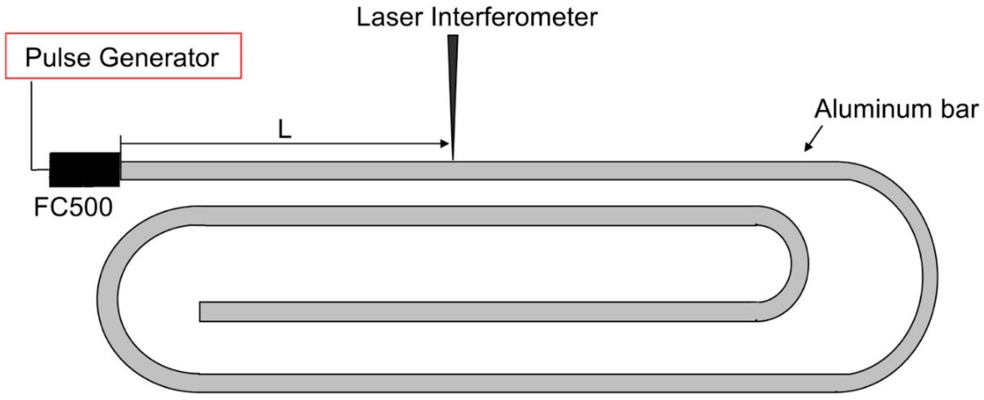
An aluminum bar of 25.4 mm × 6.4 mm × 3660 mm was shaped as shown in Figure 1. The material was UNS A96061 (6061-T6511 temper from Kaiser Aluminum, Spokane, WA, USA) with the mass density of 2.70 Mg/m3, the longitudinal wave velocity = 6.42 mm/µs, and the transverse wave velocity = 3.04 mm/µs. On one end face, a transmitter (FC500 from Acoustic Emission Technology Corp., Sacramento, CA, USA) was glued using epoxy, such that guided waves produced by the transmitter were directed along the length direction of the bar. The broad face of the bar was polished and its normal displacement was determined using a laser interferometer (Thales Laser, LH-140, Orsay, France) at distance L of 300 mm from the bar end. More details on the set-up were given in reference [8]. The following changes were made in the set-up from the previous tests: (1) The pulse generator was modified, providing step-pulses of 241, 350 or 405 V with FC500 connected; (2) A different FC500 from the previous tests was used with the front alumina facing replaced by an aluminum disc of 1.6-mm thick. This disc was glued to the piezoelectric element using silver-loaded conductive epoxy. This modification reduced radial oscillations of the transmitter significantly, as will be shown later.
The response of an AE sensor was obtained by placing its center at L = 300 mm. Couplant was Vaseline and the sensor was held under 1 N force for at least 15 min before measurements were recorded. The sensor output was terminated with 10 kΩ at the input of Pico Scope (Pico Tech 3405A, Pico Technology, St. Neots, UK) and digitized at 2 ns time interval. When a sensor includes internal buffer electronics, its output was connected to a power supply and the output signal was routed to the ac-coupled scope input by a tee. No termination was used in this case as a load resistor was a part of the power supply circuit. Data analysis procedures were given previously [4,5]. Notice that signals levels in this study usually exceeded 10 mV and no cable movement occurred during measurements. No special preparation was thus required to avoid triboelectric effects, if any.
Table 1 lists AE sensors tested in this study. The transmitter data (FC500) is also shown. The nominal values of resonance frequency and sensing element diameter are given along with the model number and manufacturer. The selection of these sensors is dictated by the availability for the lack of financial resources, but most of them are commonly utilized in research and in practical applications.
3. Results and Discussion
3.1. Displacement
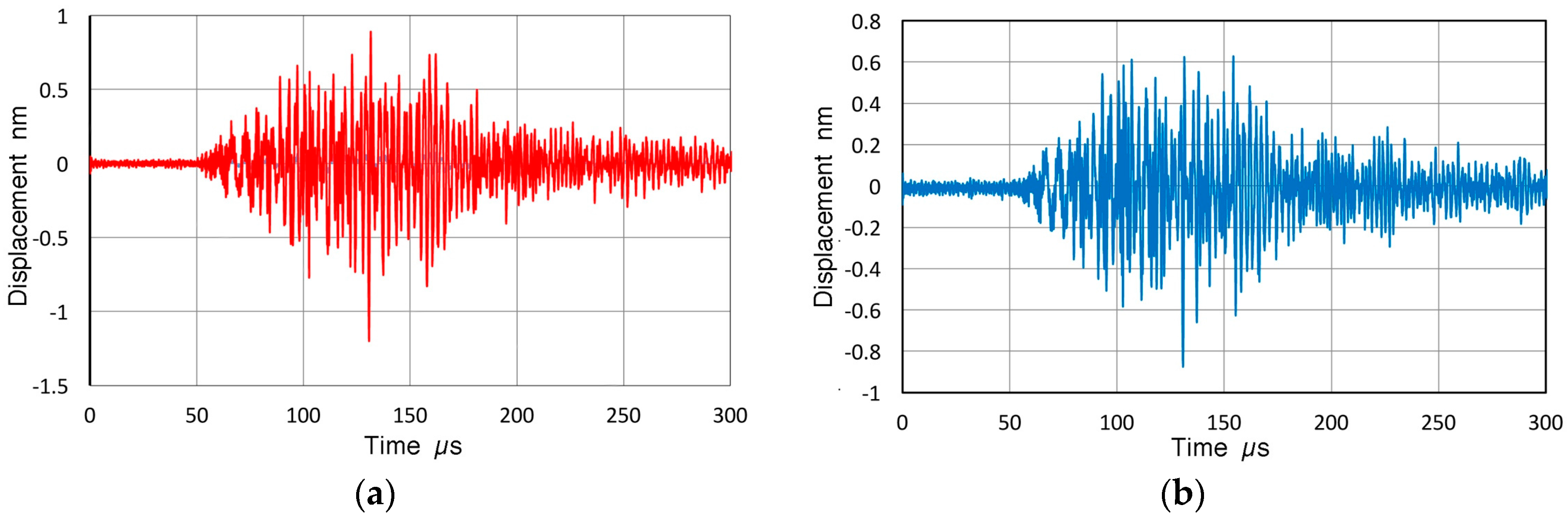
The normal displacements at L = 300 mm are shown in Figure 2a at the center and in Figure 2b at 5 mm off-center. The peak values were around 1 nm. Waveforms were similar to each other (and to that previously reported: see p. 260 of reference [8]), but the peak amplitude was about 2 dB lower at 5 mm off-center. No reflected signals were detected within the 300 µs segment. These waveforms clearly show less low frequency oscillations that were visible previously [8]. The fast Fourier transform (FFT) magnitude spectra of the displacements are given in Figure 3a,b. Figure 3a is for the center position at L = 300 mm, given in dB scale in reference to 0 dB at 1 nm (with the frequency step of ∆f = 1.90735 kHz). This spectrum peaked at 94.7 dB at 336 kHz and decreased sharply below 120 kHz. The spectral intensity above 1 MHz was also low. In the previous testing, the low frequency region below 120 kHz showed an increase of more than 30 dB (p. 261 in reference [8]). The new transmitter produced less effects of radial resonance that contributed to the low-frequency rise observed previously. Figure 3b shows five displacement spectra at 300 mm obtained at the center, 1, 2, 3 and 5 mm off-center). While the data scatter was ±5 dB or more (less scattering below 500 kHz), the average spectrum, shown by the red curve, represented the general trend well.
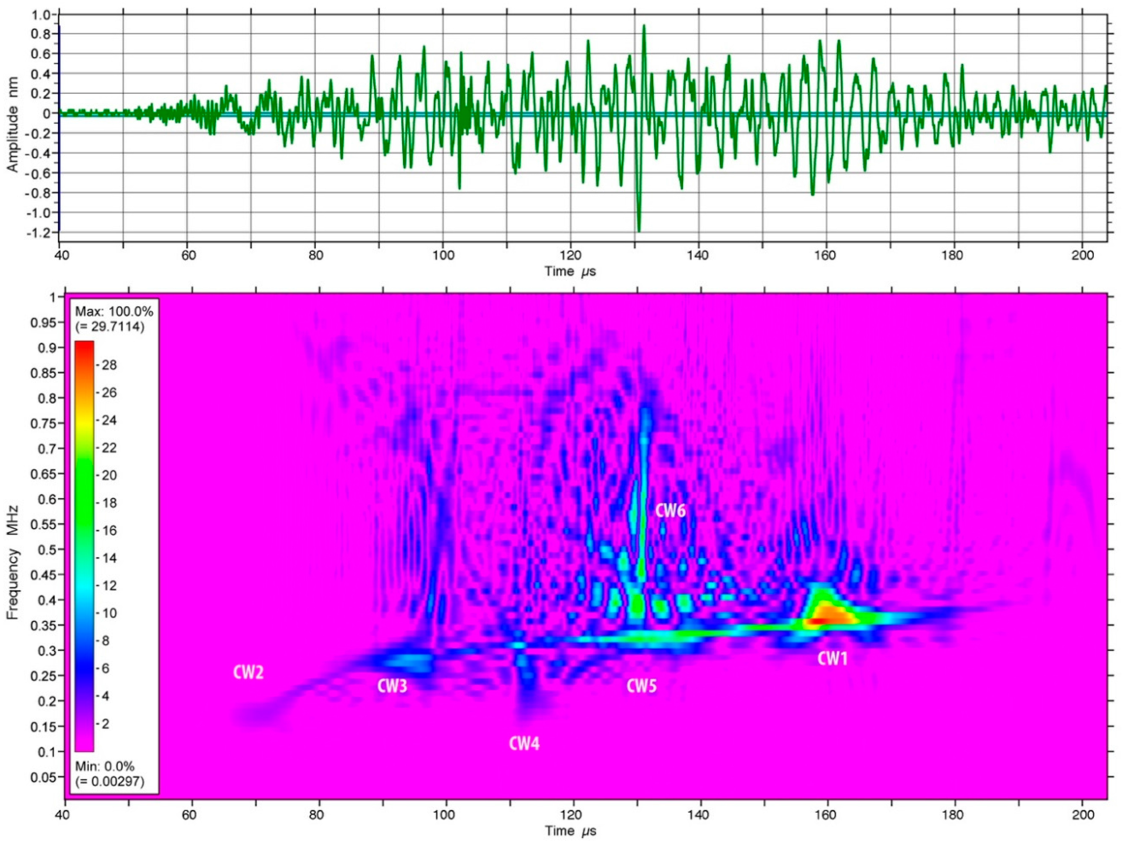
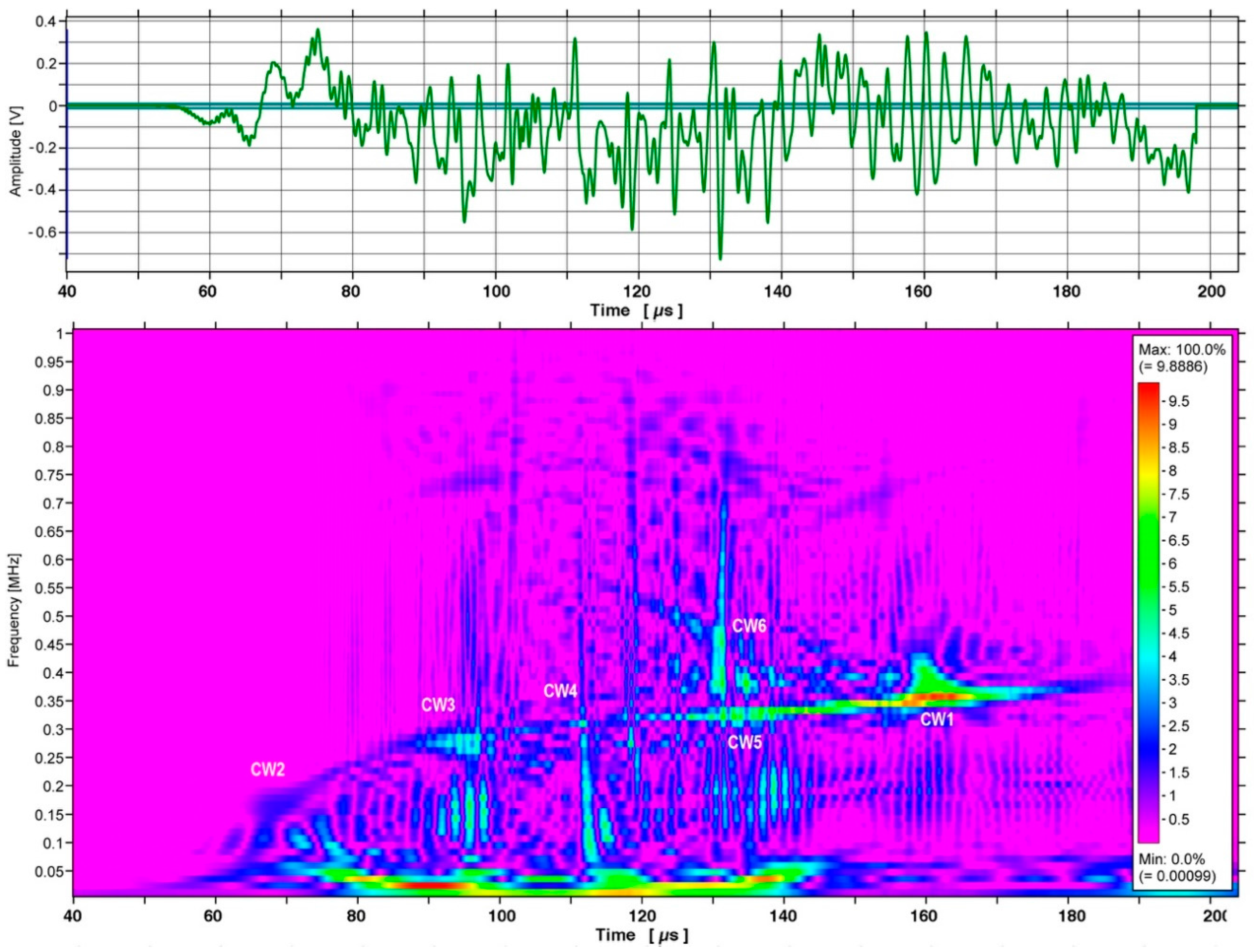
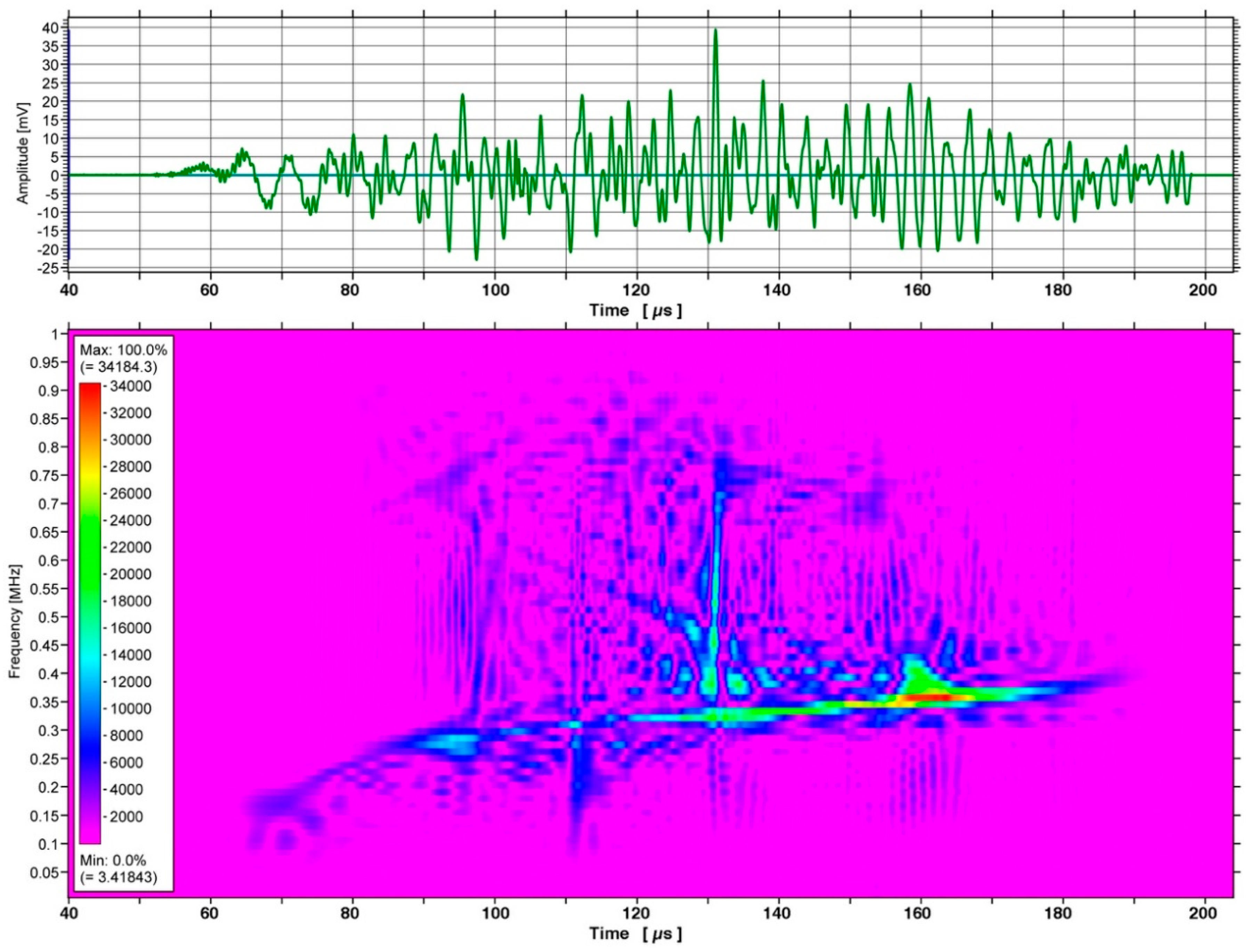
The Choi-Williams transform (CWT) was applied to the displacement waveform (Figure 2a) using AGU-Vallen Wavelet Transform software (Vallen Systeme, Icking, Germany). Figure 4 shows an expanded waveform (of the 40–200 µs segment or 7.5–1.5 mm/µs in terms of wave velocity) and time-frequency spectrogram below 1 MHz. The highest peak intensity was found at 160 µs and 350–400 kHz and marked cw1. At L = 300 mm, this peak corresponds to 1.9 mm/µs propagation velocity. A faint trace is visible from the initial weak peak at 70 µs (corresponding to 4.3 mm/µs, marked cw2) and 150–200 kHz to the main peak (cw1), passing through peaks marked cw3, cw4 and cw5. A few other traces may exist, but these traces are quite faint, except a vertical line at 130 µs (2.4 mm/µs), stretching from 400 to 800 kHz (marked cw6). The spectral intensity below 100 kHz was weak in this plot.
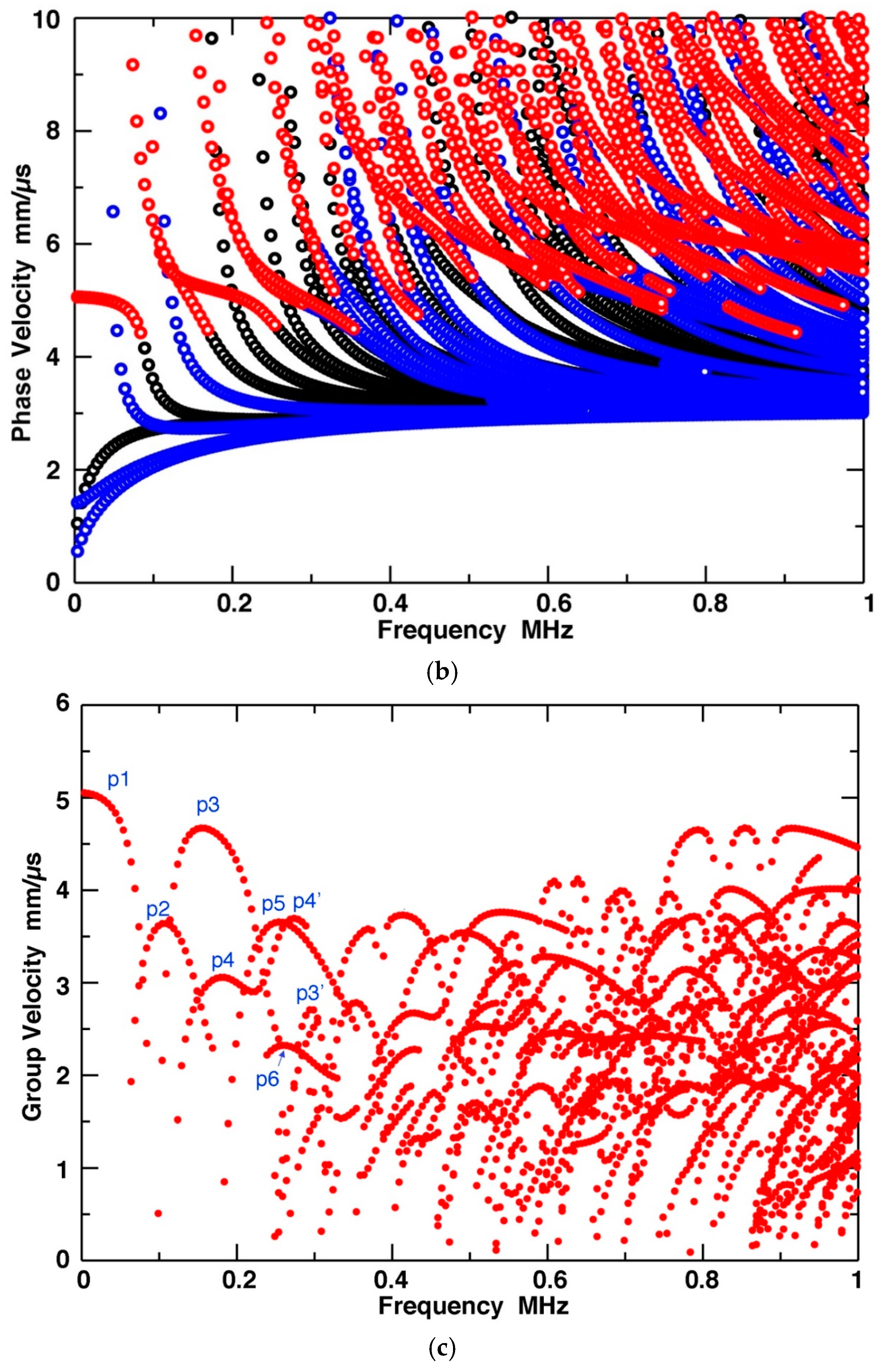
The dispersion curves for bar waves using the parameters for the present experiment are shown in Figure 5. This calculation utilized the theory and semi-analytical finite-element (SAFE) algorithm developed by Hayashi et al. [9]. The present SAFE calculation utilized 16 × 4 elements as shown in the insert of Figure 5a that indicated the directions where z refers to the bar length, y the bar thickness and x the bar width, respectively. Frequency step was 5 kHz and calculations were for 5–1000 kHz. In Figure 5a, calculated group velocities for bar waves are shown together with that of S0-mode plate wave for 6.4 mm-thick Al. The bar-wave data are divided into three types: red points represent the modes dominated by z-direction displacement, blue points those by y-direction displacement and black points those by x-direction displacement. The corresponding phase velocity dispersion curves are given in Figure 5b, using the same color codes, while Figure 5c provides the group velocity data only for the z-displacement dominated modes.
Because of the complexity, no standard naming of wave modes is available. In Figure 5c, six initial peaks are indicated by pn (n = 1–6) and with a prime for a subsequent peak of the same mode. The two lowest modes, p1 and p2, were absent in Figure 4. The next mode, p3, appears to correspond to the weak cw2 peak in Figure 4, since the velocity at the initial arrival of cw2 (4.6 mm/µs) is close to the calculated p3 peak velocity of 4.7 mm/µs. The positions of p4’ and p5 peaks match well to the arrival of cw3 (3.5 mm/µs and 280 kHz). Similarly, the position of p3’ peak matches well to the arrival of cw4 (2.7 mm/µs and 310 kHz). This p3’ mode (and perhaps p6 mode) appears to fit the position of cw5. At the position of cw1 maximum intensity peak, three or four dispersion curves are present and are likely to contribute to the cw1 peak. However, these curves are difficult to trace to the lower frequency modes. At the position of cw6 (2.4 mm/µs), a concentration of many modes exists from 470 kHz to 1 MHz. Again, these modes are difficult to identify. The nature of cw6 peak is examined further in the following section and in Appendix A.
From the CWT spectrogram and the dispersion curves, it is seen that the number of observable modes becomes large above 500 kHz. Many modes at lower velocities extend displacement signals to 200 µs and beyond and reduce the amplitude.
The dispersion curves given in Figure 5 can be scaled in terms of frequency when the ratio of thickness to width remains identical. When the thickness and width are doubled, the frequency is halved. This behavior is common with other dispersion curves for guided waves and the above results can be utilized when other bar dimensions are selected while keeping the thickness-to-width ratio of 0.25.
3.2. AE Sensor Response
3.2.1. KRN Sensor
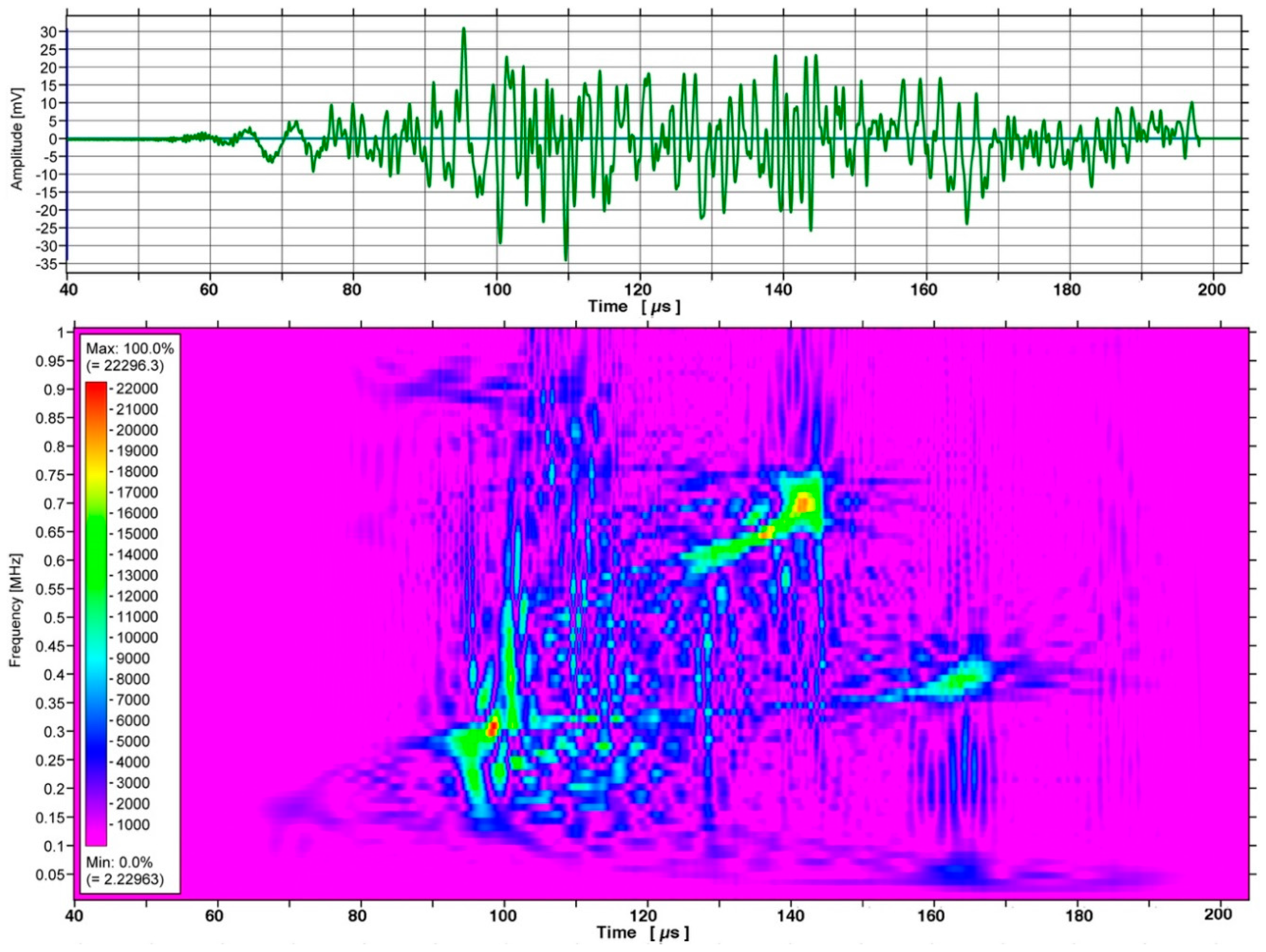
Two KRN sensors (KRNBB-PC #11053 and #11063: with a field-effect transistor (FET) buffer) were positioned at L = 300 mm with the output connected to a preamplifier/power supply (KRN AMP 1BB-J). These were made by KRN Services, Richland, WA, USA. The preamplifier section was not used since it was saturated. These sensors have a small diameter of 1 mm sensing area, approximating a point-contact sensor. The output waveform (#11063) and its CWT spectrogram are shown in Figure 6. Overall, this resembles Figure 4 and all the peaks (cw1 to cw6) appeared at the corresponding positions. Extra traces are also visible as well. In Figure 6, however, strong spectral intensities exist below 50 kHz unlike in Figure 4. This is the zone where bar-wave modes are those of x- and y-displacement dominated modes, seen in Figure 5a. This low-frequency response was, in part, a result of FET use since KRN sensors without FET showed low spectral intensities below 100 kHz (see Appendix B, Figure A4 in particular). As will be discussed later in Appendix D, the use of a coaxial cable and 10 kΩ termination of the non-buffered sensors also contributed to reduced sensitivities at lower frequencies below 300 kHz.
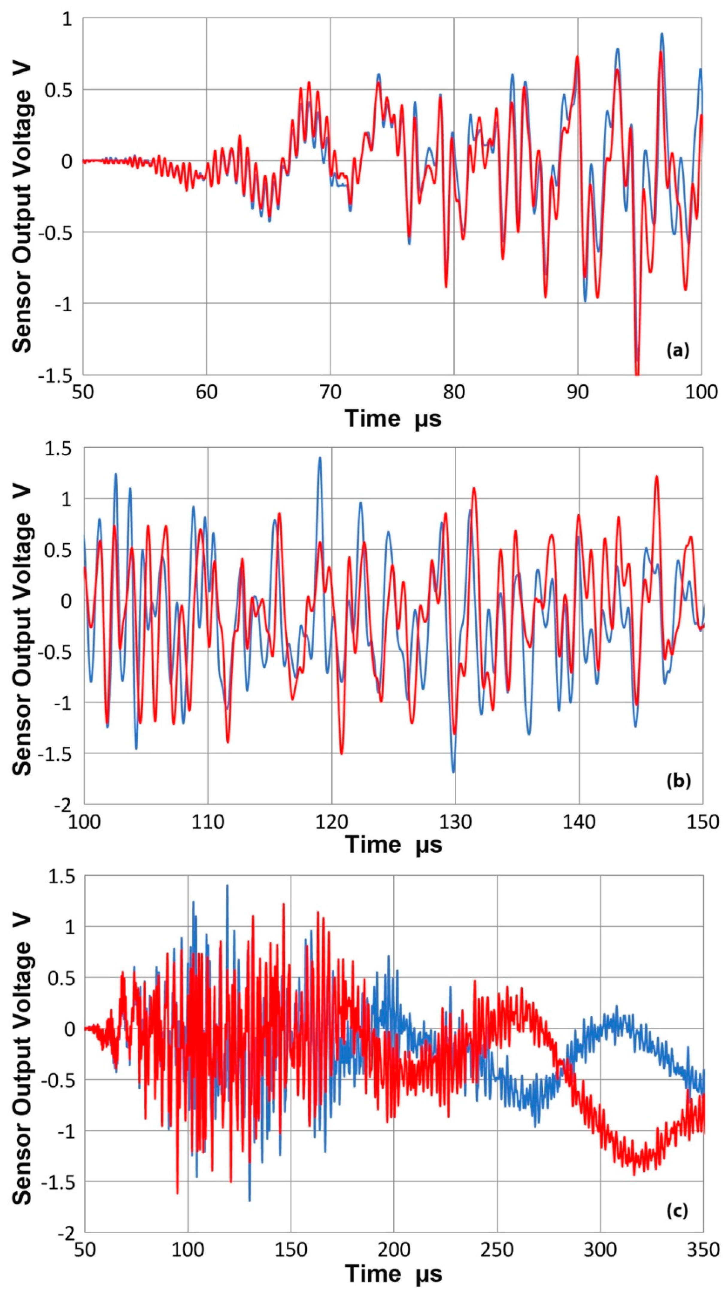
The appearance of cw6 in Figure 4 and Figure 6 was different from other peaks as it showed a constant wave velocity. By placing a KRN sensor on the top or bottom surface of the test bar, the observed waveforms were compared, as plotted in Figure 7. Starting from the wave arrival at 52 µs, most of the peak positions of the waveforms detected at the two surfaces (blue: top surface, red: bottom surface) matched well to 150 µs (shown in Figure 7a,b). That is, the wave modes are symmetric to 150 µs. Consequently, the position of cw6 is still where the symmetric modes are dominant and this peak is likely to be a combination of multiple modes, dominated by the z displacement. The possibility of this peak to be from asymmetric plate modes or from the SH mode can be discarded. (Appendix A also shows that asymmetric wave excitation did not produce this peak, further supporting its origin to be of symmetric modes.) As shown in Figure 7c, the two curves diverged beyond approximately 150 µs, implying the dominance of slow asymmetric modes at wave velocity below 2 mm/µs. This means asymmetric modes are produced even with the use of a symmetric wave excitation method. Sensitivity of propagated plate wave signals to the position of displacement input was already recognized by Hamstad et al. [10] in their three-dimensional finite-element modeling of plate waves.
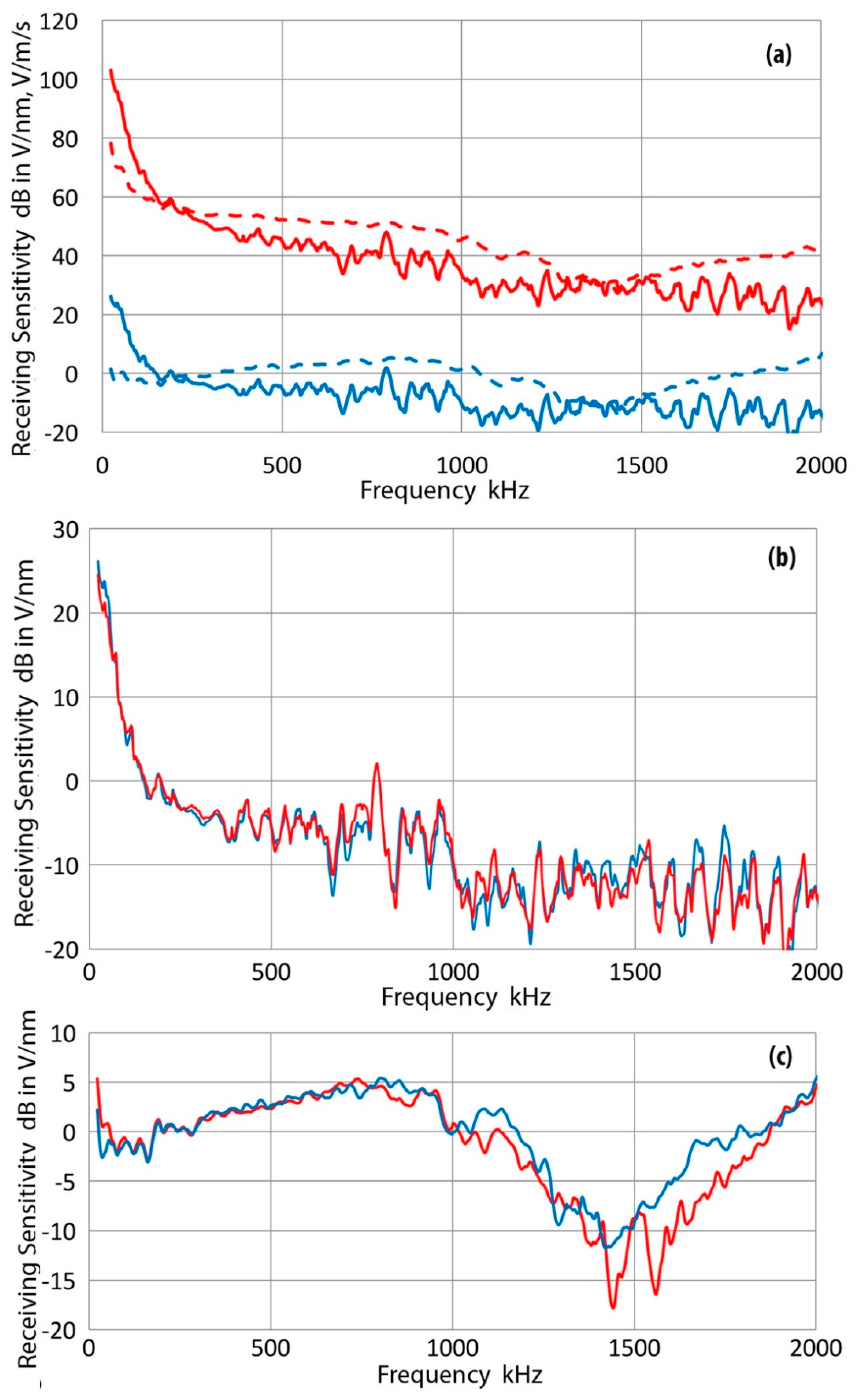
Receiving sensitivity was obtained by subtracting the center-point displacement magnitude spectrum from the output-voltage magnitude spectrum of a KRN sensor, in the same manner as in the previous studies [4,5]. Results are given in Figure 8a for #11063. Here, the displacement receiving sensitivity is given in dB in reference to 0 dB at 1 V output per 1 nm of normal displacement, shown in blue curves. Solid line is for the bar-wave data, while dashed blue curve is the displacement receiving sensitivity to normally incident waves. The latter was determined using Olympus V192 as a transmitter [4]. Note that this KRN sensor has the peak sensitivity level of about 15 dB higher than those without FET (reported in Figure 6c of reference [4]) even though the latter was measured using 100 MΩ input impedance of a 100× probe. (More sensitivity loss (of approximately 10 dB) occurs when a 60 cm long microdot cable is used between the FET-less KRN sensor and digital oscilloscope input, as will be discussed in Appendix B.)
The bar-wave sensitivity was highest at 22 kHz and decreased 30 dB to 300 kHz, above which it was relatively flat to 1.4 MHz. The normally incident wave sensitivity was flat within ±4 dB up to 1.2 MHz and differed most from the bar-wave sensitivity at frequencies below 100 kHz. The averaged normally incident wave sensitivity observed here was 1.14 dB between 22 kHz and 1.2 MHz. This compares well to the value reported by McLaskey and Glaser [11], who obtained a similarly flat response of approximately 0 ± 2 dB between 20 and 900 kHz (relying on theoretical models of capillary break or ball drop). Notice that these results are inapplicable to FET-less KRN sensors [11]. Also note that the NIST conical sensors have −9 dB theoretical and −14 dB experimental peak sensitivity [12,13]. Thus, the FET buffer in these KRN sensors apparently adds about 15 dB gain (when used with a KRN power supply).
Red curves in Figure 8a represent the corresponding velocity sensitivity curves. The velocity receiving sensitivity is given in dB in reference to 0 dB at 1 V output per 1 m/s. Again, the solid one is for the bar-wave sensitivity and dashed for normally incident. Higher frequency dependence is due to spectral differentiation with the multiplication of 2πf with f = frequency.
Figure 8b,c show the displacement sensitivity curves for bar waves and normally incident waves of two KRN sensors tested. Red curve is for #11053 and blue curve is for #11063. In these figures, the curves for #11053 were down-shifted 4.4 dB (Figure 8b) and 3 dB (Figure 8c), achieving good matching of the two curves. In Figure 8b, both bar-wave curves rose by 30 dB below 300 kHz, while these were relatively flat from 300 kHz to 1 MHz except for many fluctuations. Many of them are observed at the same frequencies for both. The sensitivities further decreased at >1 MHz. The difference between these two sensors was 4.4 dB on average to 2 MHz (with the standard deviation of 1.46 dB). Figure 8c gives a comparison of displacement sensitivity curves for normally incident waves. The average difference to 1 MHz was 3.0 dB (1.8 dB to 2 MHz); that is, #11053 had a higher sensitivity. These are smoother below 1.2 MHz than the bar-wave responses.
The present results clearly demonstrate that the receiving sensitivities to bar waves and to normally incident waves are different even when the sensing area is small. This confirms that the direction of wave propagation affects sensor response in addition to the well-known aperture effect or waveform cancellation effect [2,14,15,16]. In reference to surface waves, the aperture effect predicts nulls at the zeroes of Bessel function of the first kind, J1(ka), where k = 2πf/cR, cR = Rayleigh wave velocity and a = radius of the sensor element [2]. The values of ka for the first four nulls, where J1(ka) = 0, are 3.832, 7.016, 10.173 and 13.324. In the present case, the wave velocities are those of bar waves and these typically exceed 2 mm/µs. For KRN sensors, a = 0.5 mm. Thus, the aperture effect has no consequence below 2 MHz. It is expected that a conical element used in NIST-type sensors responds to forces acting at incident angles other than zero. A better analysis of such behavior is desirable.
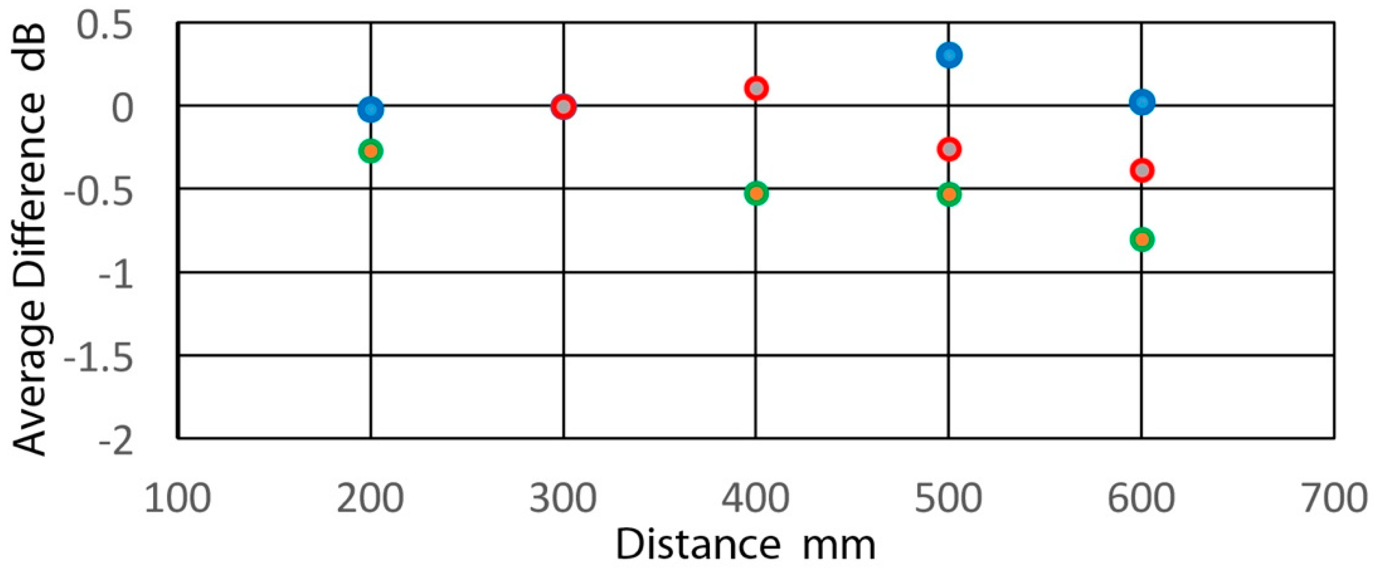
In the present study, displacement measurements were only made at L = 300 mm. Effects of changes in L on the integrated intensity were examined using two KRN sensors (without FET) at different L values from 200 to 600 mm. Results are given in Figure 9 using the average of spectral values over equivalent signal ranges; i.e., 27–133 µs for L = 200 mm to 120–400 µs for L = 600 mm. The changes were small, mostly less than 0.5 dB. That is, displacement signals attenuated little except by dispersion (signal spreading) effect, especially below 1 MHz.
Practical consequence of the present finding is that one needs to avoid using conventional face-to-face calibration results in selecting sensors for detecting guided waves. This aspect has been noted from the early days of AE testing [1]. However, the surface wave calibration for most commercial AE sensors has generally been unavailable, resulting in inadequate recognition of the aperture effect and of the needs of guided wave calibration data.
3.2.2. Other Small-Diameter Broadband Sensors
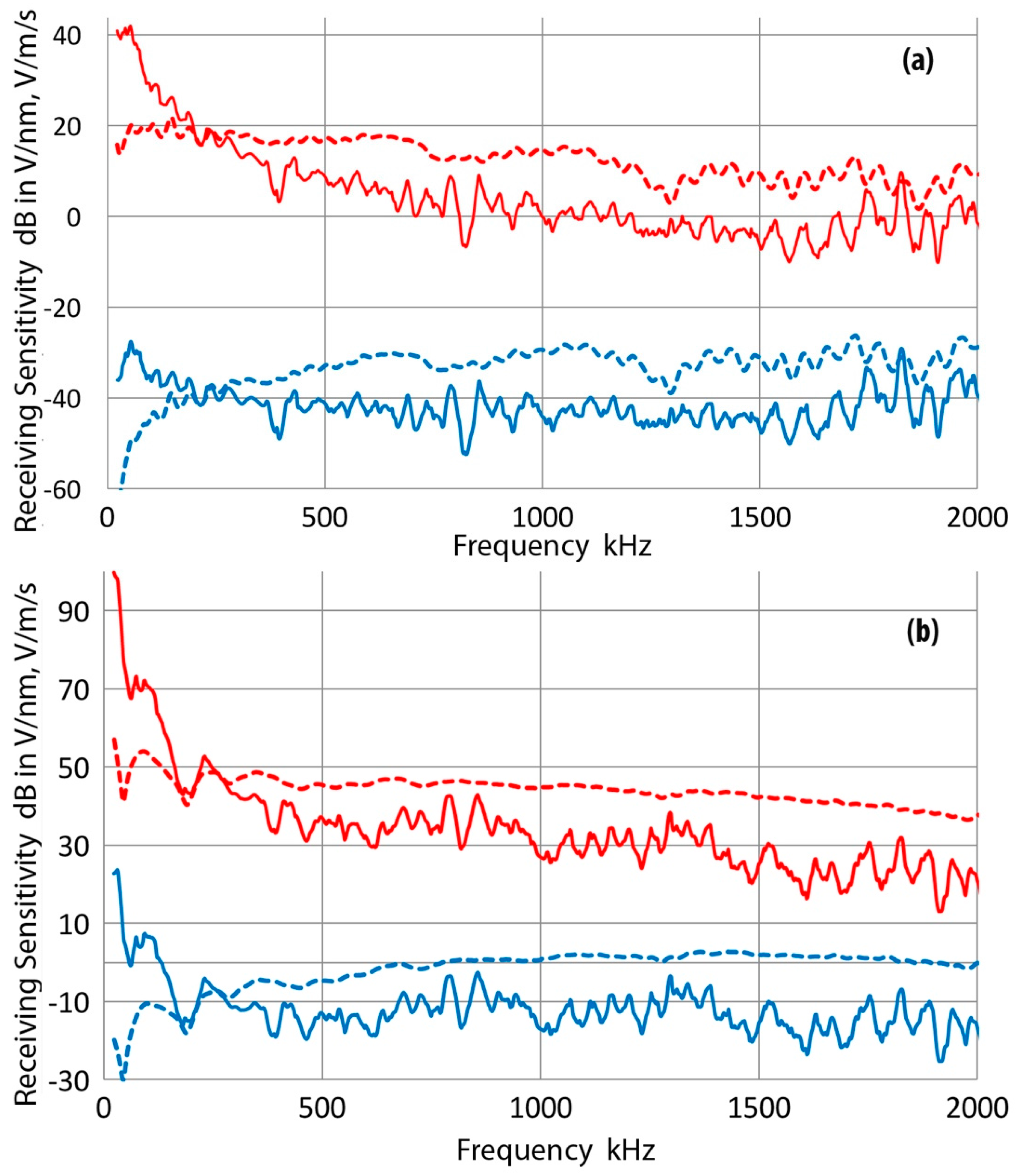
Two broadband sensors with a small sensing area were tested. These are Valpey-Fisher (now CTS-Valpey, Hopkinton, MA, USA) Pinducer and Digital Wave Corp. (DWC, Centennial, CO, USA) B1080-LD. The Pinducer was of VP-1093 design with the element diameter of 1.35 mm, but had a quarter-wave matching layer (140 ns delay time). Figure 10a gives its receiving sensitivities using the same color code as in Figure 8a. The sensitivity levels are 30–40 dB lower than those of KRN (with FET) sensors, but spectral flatness for the bar-wave sensitivity is improved by 20 dB or more (in terms of the range of sensitivity).
As shown in Figure 10b, DWC B1080 sensor, which has an FET buffer, has sensitivity levels comparable to KRN sensors, but it has a nominally 3.2-mm element diameter, or about ten-times larger sensing area. Its normally incident velocity sensitivity is flat within ±3 dB from 200 kHz to 1.5 MHz. This sensor also has sharply rising low-frequency bar-wave sensitivities.
Here, it is worth noting that another miniature sensor design was developed with capacitive sensing principle. Kim et al. [17] used a circular sensing electrode of 1.8 mm diameter, mounted inside a cylindrical housing of 12 mm diameter and 32 mm length. Although no sensitivity characteristics were given, they successfully recorded nanometer-level glass-capillary fracture signals.
3.2.3. PAC R6a Sensor
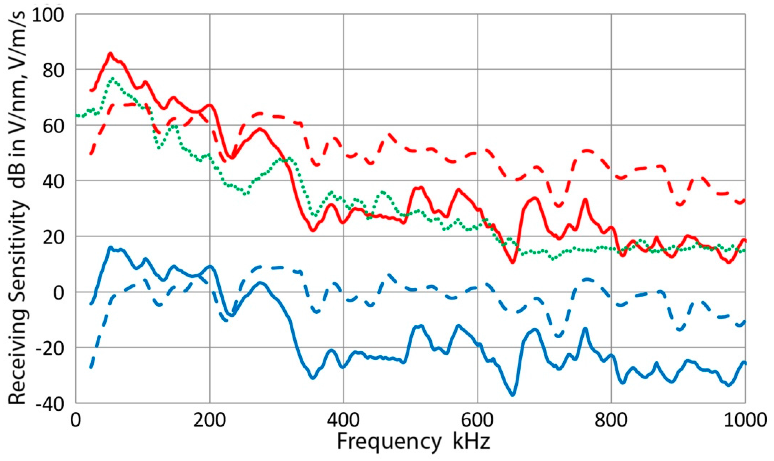
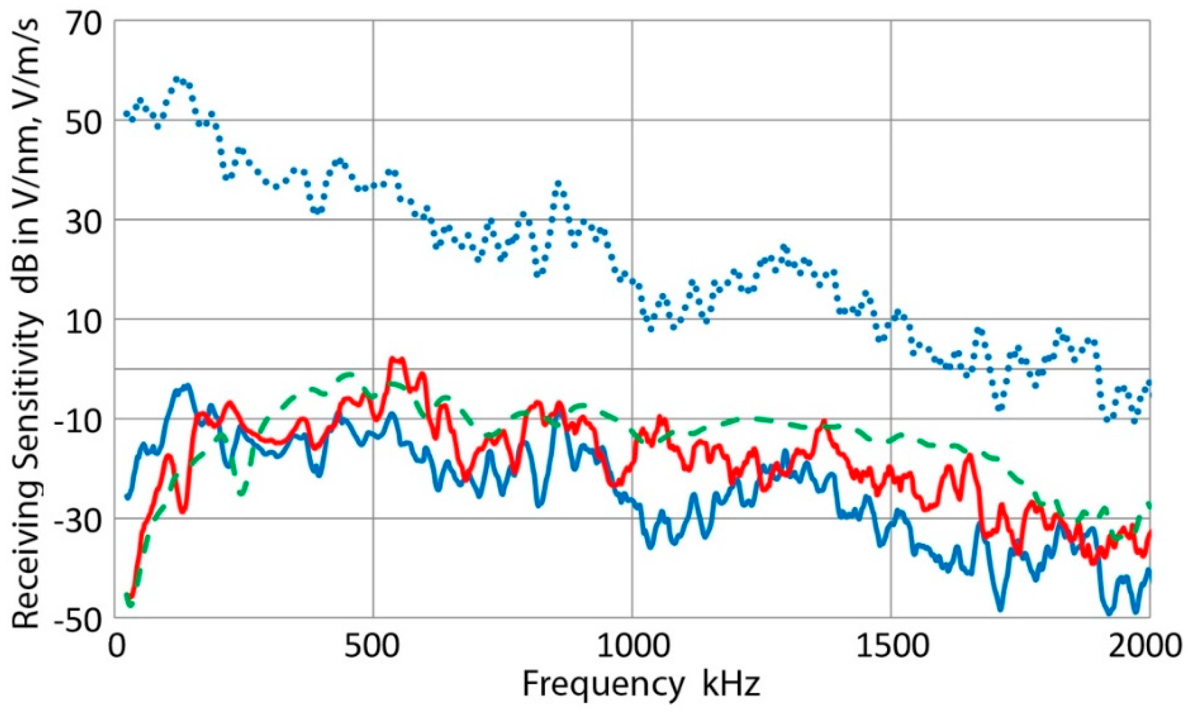
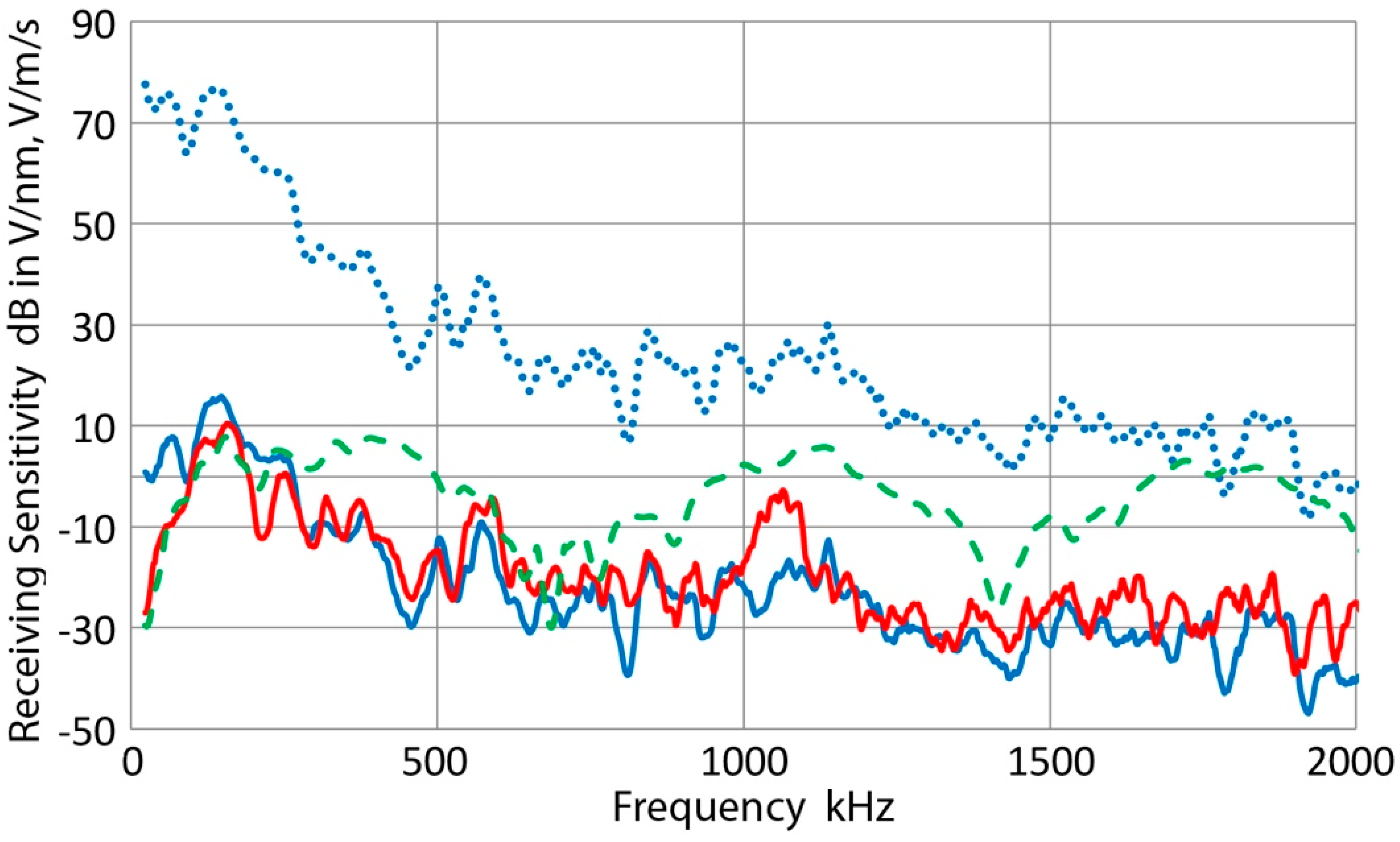
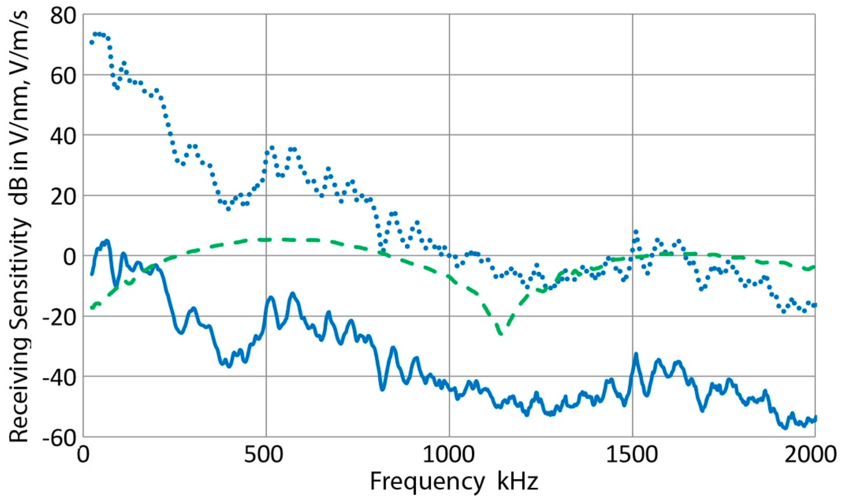
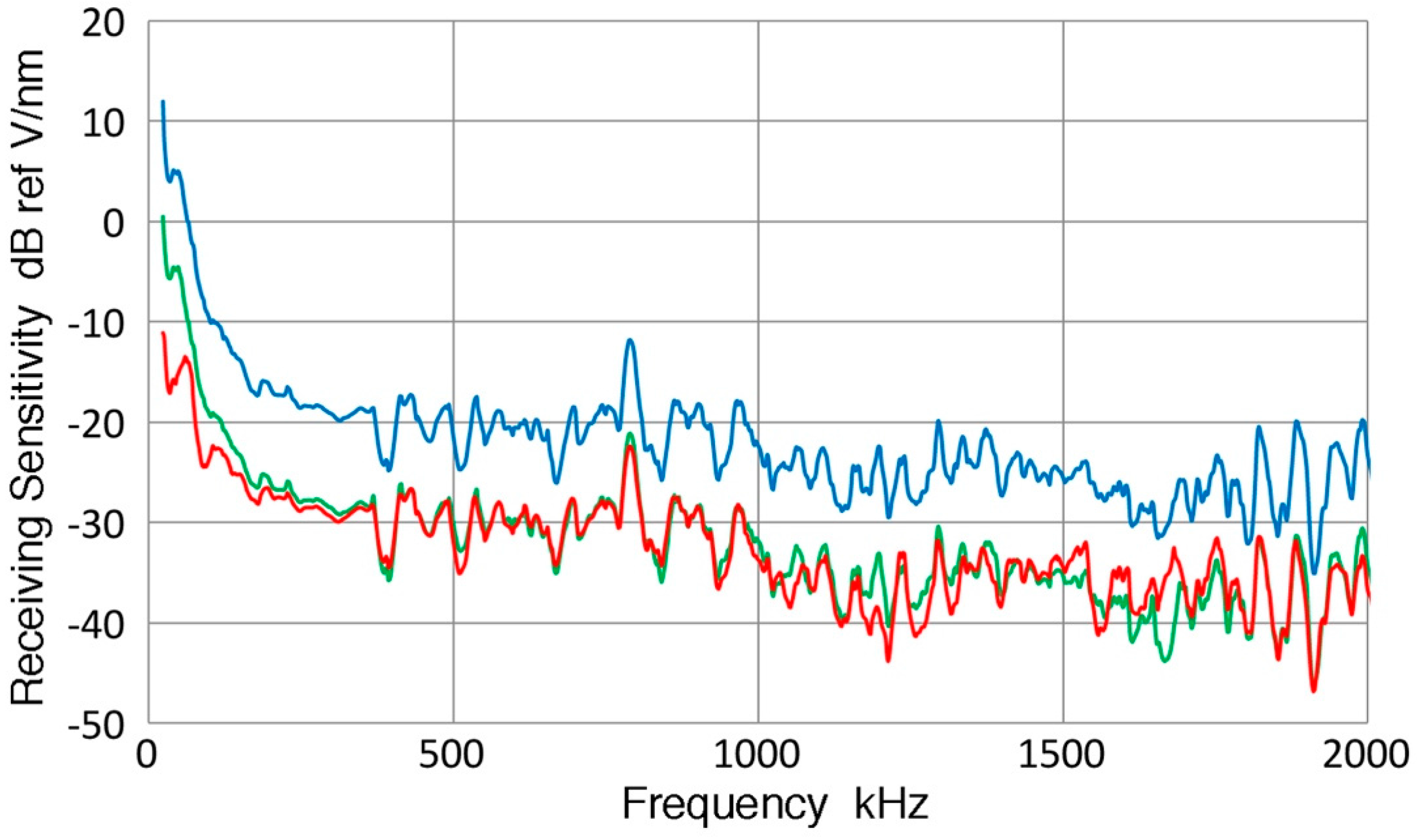
This sensor is a nominally 12.7 mm diameter design for low frequency applications and was supplied with a surface-wave velocity calibration by the manufacturer (Physical Acoustics Corp. or PAC, Princeton Junction, NJ, USA). Thus, it is appropriate to compare our bar-wave calibration result to the PAC calibration. Measurement was taken at L = 300 mm; that is, the center of an R6a is placed at this distance. The receiving sensitivity was obtained by subtracting the averaged displacement magnitude spectrum (the red curve in Figure 3b) from the output-voltage magnitude spectrum. Results are shown in Figure 11. The solid blue curve is the bar-wave displacement sensitivity and the dashed blue curve is the normally incident wave displacement sensitivity. Note that the latter exhibits a broadband response from 50 kHz to nearly 900 kHz with the highest peak at 277 kHz. Again, these two are of similar magnitude, but the bar-wave displacement sensitivity has a higher frequency dependence, peaking at 16 dB at 52 kHz. The corresponding velocity sensitivity (red curve) has the maximum sensitivity of 86 dB, also at 52 kHz. The manufacturer’s surface wave data (green curve) was available to 1 MHz and peaked at 77 dB at 54 kHz with a good spectral shape matching to the bar-wave result up to 1 MHz, except over 150–300 kHz. Three additional R6a sensors were similarly tested and their results are given in Appendix C. The similarity of bar-wave and surface-wave velocity sensitivity was also observed. The average peak sensitivity difference of the four tested R6a was 9.0 dB, while the peak frequency difference was 1.9 kHz.
While details of the surface-wave calibration provided by PAC are not available, it is concluded that the present method provides a practical approximation of the surface-wave calibration data without the need of a large calibration block, but on the basis of verifiable laser interferometer measurements. It should be noted that the NIST AE-sensor calibration service was closed for more than ten years. Thus, the reference standards at various manufacturers are most likely out of date at this time and the present bar-wave calibration method can be substituted in the absence of the NIST standard.
3.2.4. Olympus V103 Transducer
This transducer is a nominally 12.7 mm diameter, 1 MHz design for ultrasonic applications from Olympus NDT, Waltham, MA, USA, but is also used as a broadband AE sensor [18]. Results of bar-wave displacement calibration tests are given in Figure 12. The blue curve is from the present test, while the red curve was reanalyzed from the previous test data for Figure 12b in reference [8] (using the equivalent time period in conducting FFT). These two spectra showed large dips at 400 kHz, and at 900 ± 100 kHz. While these two curves matched reasonably well overall (except below 120 kHz, near 600 kHz and near 1.1 MHz), the low frequency data diverged. This discrepancy was also found in other sensor data (pages 15 and 18) and apparently resulted from a large effect of transmitter radial resonance that was present in the previous set-up. Higher displacement output below 120 kHz in the previous interferometer data did not produce higher sensor output. Exact cause of this effect is still unclear, however.
In Figure 12, the dashed green curve is the normally incident wave displacement sensitivity for V103 (given in Figure 9a in reference [4]). This is smoother than the bar-wave data and peaked at 1.1 MHz. This shows no dip unlike the bar-wave sensitivity curves.
The observed frequency of 400 and 900 kHz for the two major dips in Figure 12 are compared to the predictions from the nulls of J1 function. The first dip matches with the first null if the velocity is assumed to be 4.2 mm/µs. According to the bar-wave dispersion curves (Figure 5c), this velocity is 13% higher than the peak velocity of 3.7 mm/µs calculated at 400 kHz. At 900 kHz, the needed velocity is 5.1 mm/µs for the second null, while a few modes have velocity of 4.7 mm/µs, at 6% difference. These are acceptable deviations as two theoretical predictions have to be reconciled. Alternately, a combination of 2.3 mm/µs at 400 kHz and 3.6 mm/µs at 900 kHz provides a good matching for the second and third nulls. However, this choice requires another spectral dip at a lower frequency of around 200 kHz. No such dip is evident in Figure 12 and the alternate set is not viable. While the predictions are not exact matches to the bar-wave calculations, the dips can be attributed to the aperture effects.
3.2.5. PAC S9220 Sensor
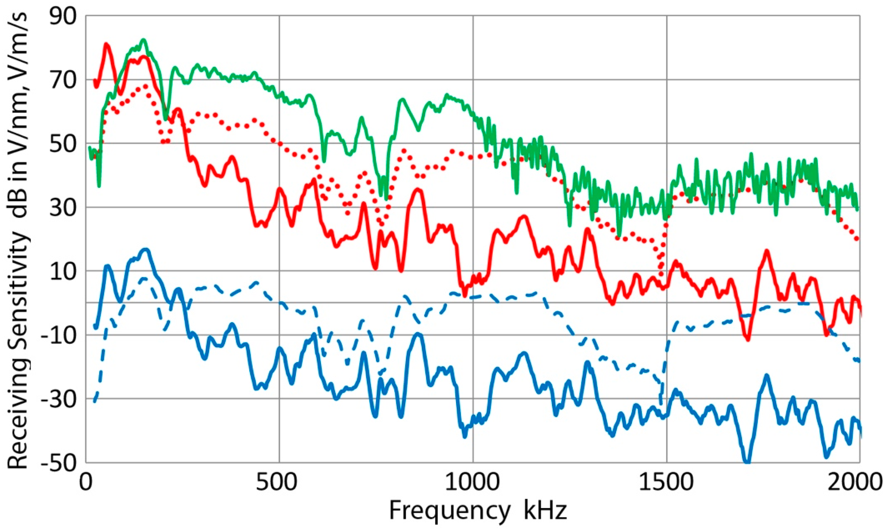
This sensor is a nominally 6 mm diameter, 900 kHz design for broadband applications. Results of bar-wave calibration tests are given in Figure 13. The blue curve is from the present displacement sensitivity test, while the red curve was reanalyzed from the previous test data for Figure 13b in reference [8]. The dashed green curve is the normally incident wave displacement sensitivity (Figure 10b in reference [4]), while the dotted blue curve is for the bar-wave velocity calibration. Again, the red curve from the previous study showed a decrease below 120 kHz due to radial resonance effect. This low frequency decrease needs to be ignored, but it is shown for completeness.
A comparison between the blue and dashed green curves points to a distinction between the guided-wave response and normally incident wave sensitivity. The latter gives a peak response at 900 kHz, while the former peaks at a low frequency. Such a difference always emerged in all the sensor evaluation so far. In the bar-wave (blue) curve, a dip is observed at 400 kHz as in V103 (Figure 12). The aperture nulling effect for this smaller sensor is expected here when the bar wave propagates at 2 mm/µs. A few modes exist in the calculated dispersion curve (Figure 5c).
3.2.6. Pico Sensor
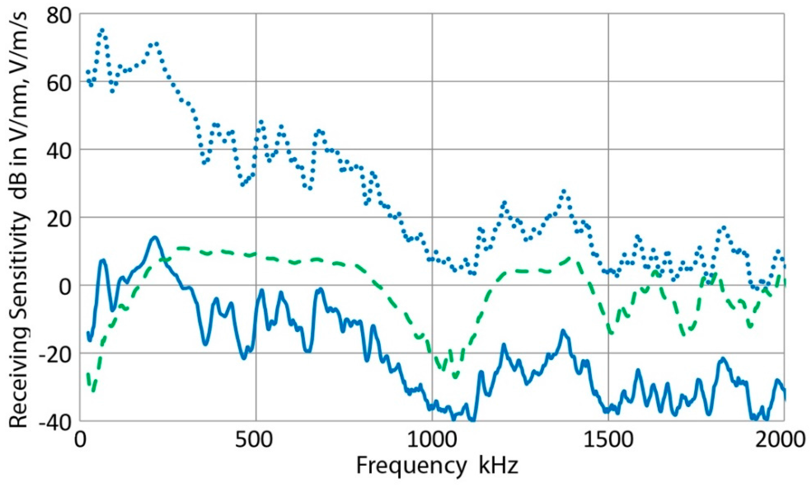
This sensor is a nominally 3.2 mm element diameter, 500 kHz design for broadband applications. Results of bar-wave calibration tests are given in Figure 14. The blue curve is from the present displacement sensitivity test, while the red curve was reanalyzed from the previous test data for Figure 13d in reference [8]. The dashed green curve is the normally incident wave displacement sensitivity (Figure 10b in reference [4]). The dotted blue curve is for the bar-wave velocity calibration. Again, the red curve from the previous study showed a decrease below 120 kHz due to radial resonance effect.
In this case, a spectral dip may exist at 1.05 MHz, but this seems to be from a scatter in the data. Because the sensor radius is small, aperture null effects are absent. In this Pico sensor, a distinction between the blue and dashed green curves or between the guided-wave response and normally incident wave sensitivity is less pronounced.
3.2.7. PAC WD Sensor
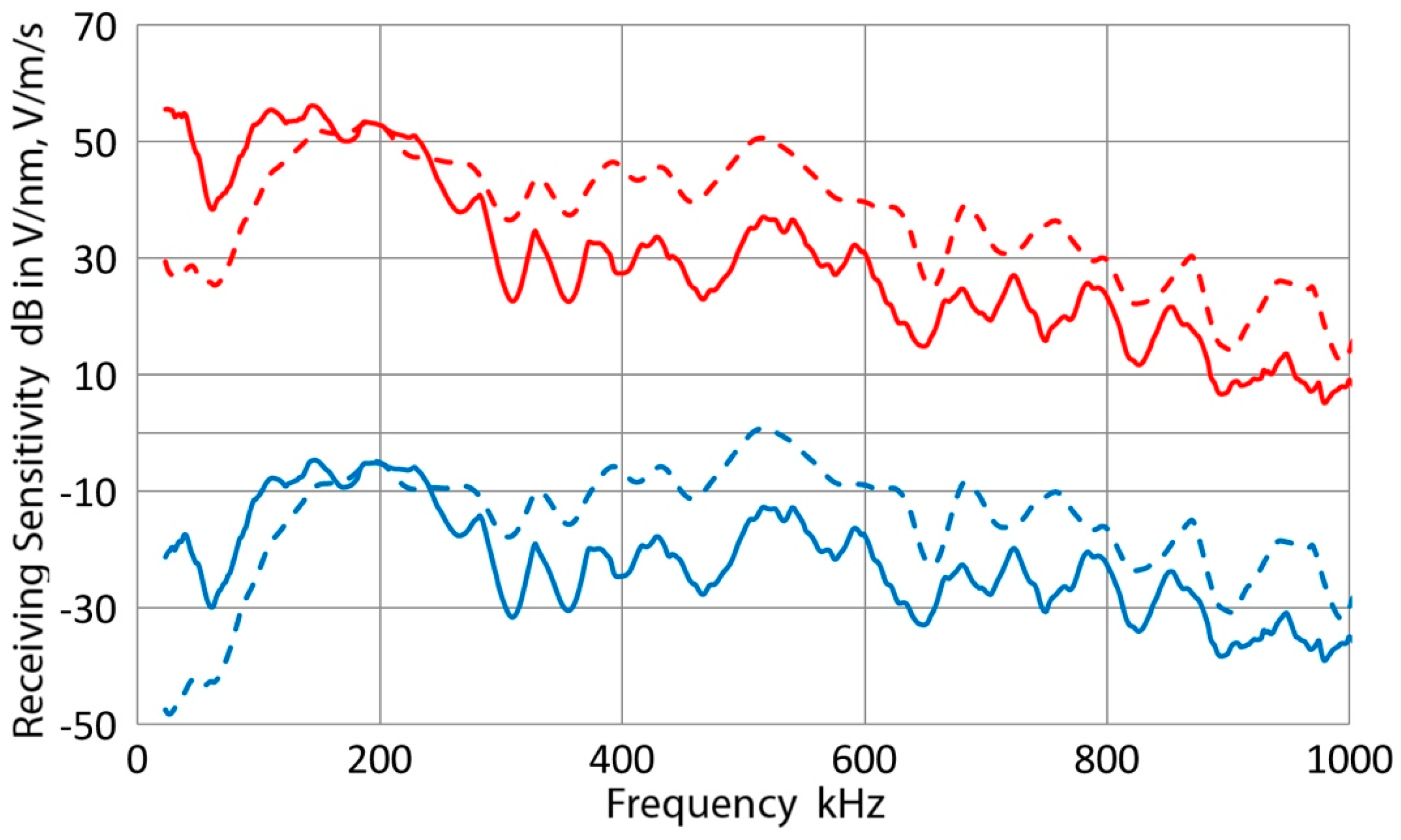
This sensor has a 12.7 mm diameter case, but is based on a multiple-element design. Results of bar-wave calibration tests are given in Figure 15 as solid curves, while those for normally incident waves as dashed curves. Color code is similar to that in Figure 11. A large dip is seen at 350 ± 30 kHz, which is similar to the first dip of V103. In this case, element size is difficult to estimate: taking it as 10 mm, this corresponds to 2.8 mm/µs at 350 kHz. A few bar-wave modes exist at this position in Figure 5c. As in other cases presented, this sensor again showed vastly different responses to bar waves and to normally incident waves. While the latter is relatively smooth from 200 to 1200 kHz, the same cannot be said for the bar-wave response.
3.2.8. PAC µ30D Sensor
This sensor is a nominally 8 mm element diameter, 300 kHz design. Results of calibration tests are given in Figure 16. Color code of the previous figure is applicable. The blue dash curve for the normal incidence displacement sensitivity shows a useful range of 100 to 500 kHz, but for the bar waves good sensitivity range becomes limited to below 250 kHz. Here, the aperture effects are obscure as many fluctuations are present above 400 kHz.
3.2.9. PAC HD50 Sensor
This sensor is designed to screw into a threaded hole with a small hexagonal rod housing (6.3 mm across) and with a limited sensing element size. Tested with a short, threaded-brass hexagonal rod, it showed a peak at 500 kHz to normal incident waves as the sensor designation implied (Figure 17). Again, peak response frequencies to bar waves shifted down to 100–230 kHz. The aperture effects are again obscure as many peaks and dips are present.
3.2.10. PAC R15 Sensor
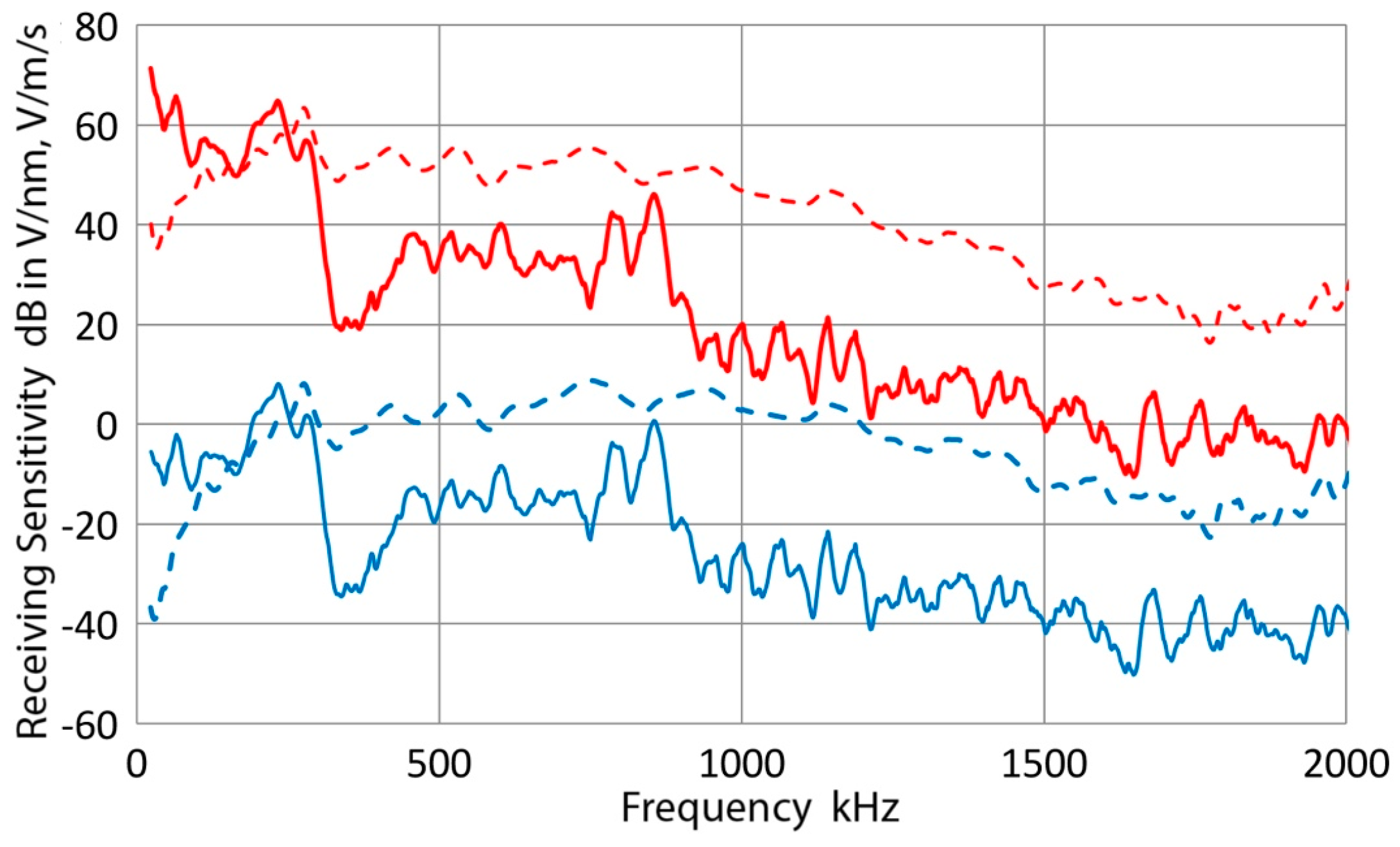
This sensor is a 12.7 mm element diameter, 150 kHz design for routine AE applications. Results of bar-wave calibration tests are given in Figure 18. The blue curve is from the present displacement sensitivity test exhibiting the maximum sensitivity of 15.8 dB at 146 kHz, while the red curve was reanalyzed from the previous test data for Figure 11 in reference [8]. The dashed green curve is the normally incident wave displacement sensitivity (Figure 10a in reference [4]), which shows peaks of similar values (approximately 7.6 dB) at 152 and 390 kHz. Another peak at 1130 kHz is only 2 dB lower. The dotted blue curve is for the bar-wave velocity calibration. The red curve showed a low-frequency drop below 120 kHz, but otherwise followed the blue curve well. Dips for the blue curve are at 460, 810 and 940 kHz and are comparable to the case for V103, another 12.7 mm diameter sensor. No corresponding decreases exist for the dashed green curve for normally incident waves.
3.2.11. PAC R15a Sensor
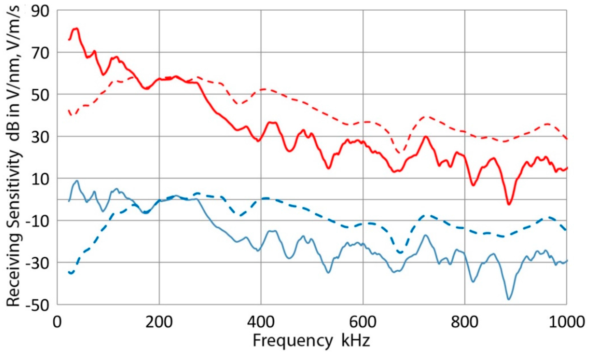
This sensor is a newer design of R15 sensor discussed in Section 3.2.10 above, a nominally 12.7 mm diameter, 150 kHz sensor for routine AE applications. Results of bar-wave calibration tests are given in Figure 19. The displacement receiving sensitivities are shown in blue curves and velocity sensitivities are in red as in Figure 17. Solid lines are for the bar-wave data, while dashed curves are for the sensitivities to normally incident waves. As was the case for R15 above, the blue curve has the maximum of 16.7 dB at 156 kHz and the sensitivity deceases as frequency increases above 300 kHz. The blue dashed curve (normally incident wave sensitivity) has a flatter response. From 100 to 1200 kHz (except 600–800 kHz), the sensitivity is mostly within ±5 dB. This can indeed be used for broadband detection. The velocity responses (red curves) reflect the displacement responses as expected. The solid green curve is the velocity calibration data provided by the manufacturer (and was converted to V/m/s scale by adding 143.4 dB [4]). From its frequency dependence, this was for normally incident wave sensitivity. As noted previously [4], such calibration data is usually overstated by 15 dB and the present result confirmed the same behavior.
The bar-wave responses are different from those of R15 sensor, except for a dip at 460 kHz. Aperture effects are difficult to interpret here, perhaps resulting from a more complex sensing element design.
3.2.12. PAC F30a Sensor
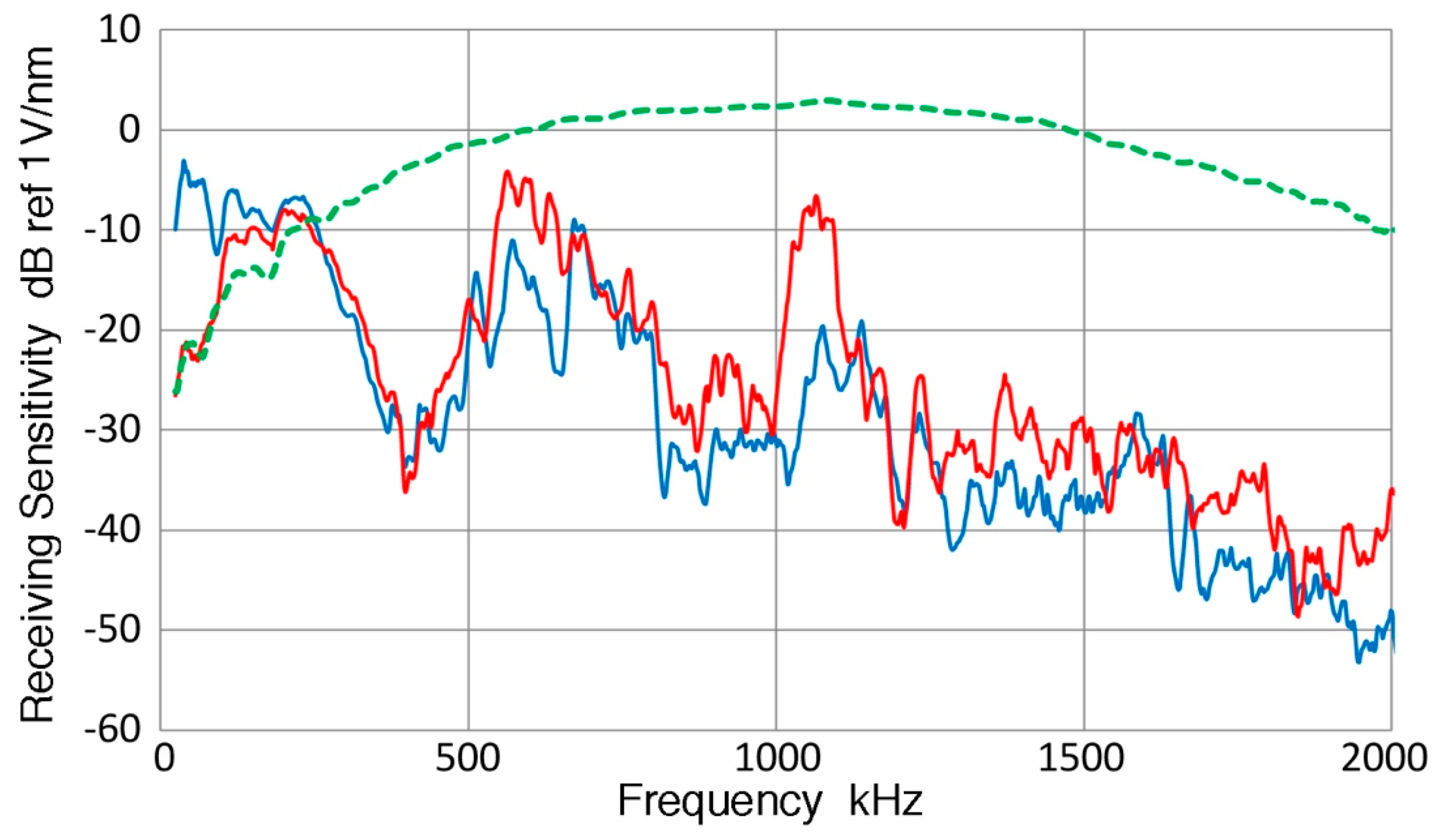
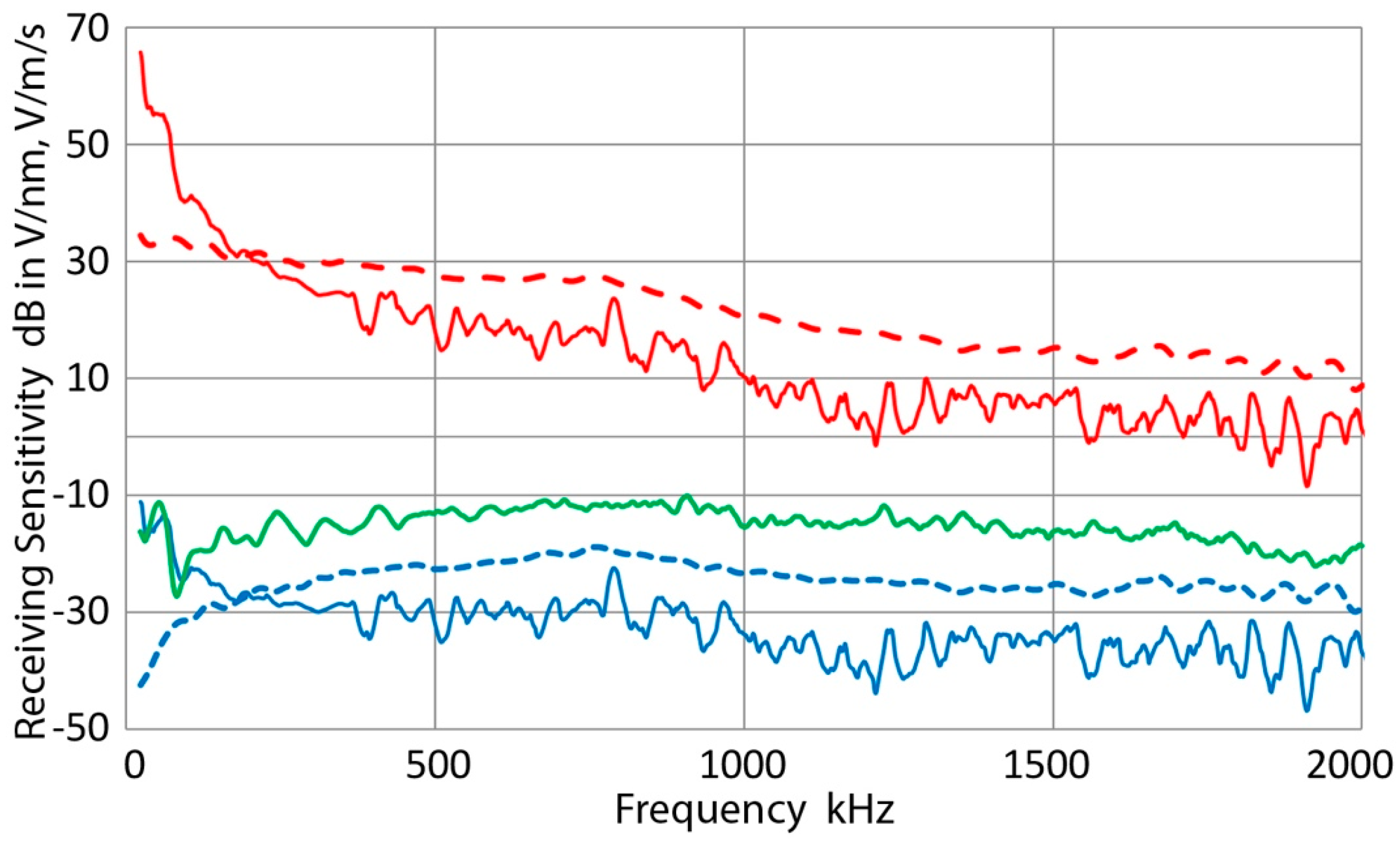
This sensor is a new design based on a composite piezoelectric element, giving a flat frequency response over 200–800 kHz in terms of the normally incident wave displacement sensitivity, as shown by the green dash curve in Figure 20. This differs substantially from the blue curve in this figure that represents bar-wave displacement calibration data. The dotted blue curve is for the bar-wave velocity calibration. The blue curve reaches the maximum of 14 dB at 212 kHz, but the peak of 75 dB for the velocity curve is achieved at 60 kHz. A dip in the spectrum exists at 1.1 MHz, but it is difficult to assess if this relates to the aperture effect without construction details.
This case most clearly demonstrates different spectral characteristics for the two types of incident waves, normally incident and guided waves, requiring a suitable selection of a sensor in an AE application.
3.2.13. DECI SH225
This shear-wave sensor was developed at Dunegan Engineering (DECI, now Score Atlanta, Kennesaw, GA, USA). It is designated to have 225 kHz center frequency for shear waves using a rectangular element. The shear motion is along the short direction. As shear wave sensitivity is difficult to define or measure, the same test methods were used as in all other tests. Results are given in Figure 21. Displacement sensitivity is surprisingly good and broadband for normal incidence (blue dashed). Only low-frequency sensitivity below 100 kHz is usable for bar-wave detection. For this test, bar waves propagated along the short direction of the sensing element.
3.2.14. Olympus V101 Transducer
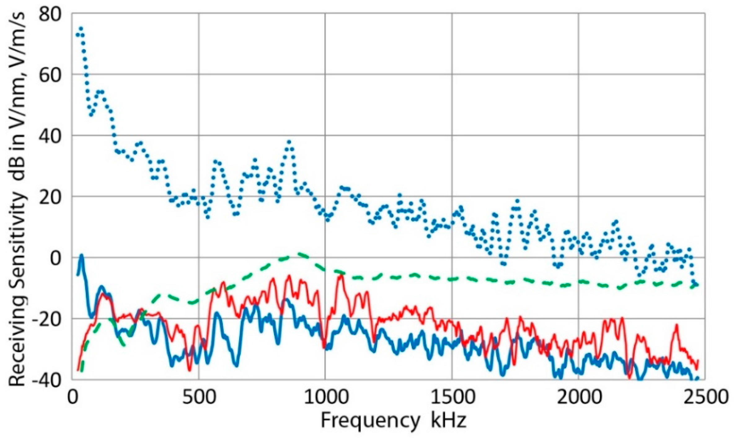
This transducer is a nominally 25.4 mm diameter, 0.5 MHz design for ultrasonic applications. This was used in our calibration studies and is unlikely to be used as an AE sensor. However, its larger size offers a comparison to smaller sensor sizes in considering wave cancellation effects. Bar-wave responses in displacement (solid blue) and velocity (dotted blue) are shown in Figure 22. Both of the blue curves peaked at 63 kHz, giving 5.1 dB (displacement) and 73 dB (velocity). The bar-wave displacement response drops off sharply at 200 kHz and this sensor is useful only for the low frequency (large wavelength) region. The dashed green curve gives the displacement sensitivity to normally incident waves with a broad maximum of 5.3 dB at 550 kHz and a dip at 1.15 MHz, giving a useful range from 150 kHz to 1 MHz.
For the bar-wave curve (blue), a dip appears at 380 kHz. This corresponds to the second null for wave velocity of 4.3 mm/µs or for the third null for wave propagating at 3.0 mm/µs. The dispersion curves (Figure 5c) show a mode at 3.4 mm/µs and a few modes at 2.7 mm/µs, so the third null appears to produce the observed dip. A minor dip exists at 270 kHz, corresponding to the second null for the velocity of 3.0 mm/µs. A dip for the first null is absent, however. Thus, the aperture effects again caused the dips in V101.
3.3. Further Discussion
Results given above lead to the following observations.
- Receiving sensitivities to bar waves and to normally incident waves are different for any given sensor.
- Differences in the sensitivities to bar waves and to normally incident waves increase with the increase in frequency above approximately 200 kHz with the bar-wave sensitivity becoming lower at higher frequencies. In the low frequency range, the opposite is usually observed; that is, the bar-wave sensitivity is higher.
- The differences at higher frequencies noted in b. above are smaller when the sensing area of the sensor is small, as in KRN and Pinducer sensors. In contrast, the differences are larger for larger sensors, like V101 and V103.
- Even when spectral flatness exists for the receiving sensitivity to normally incident waves, the receiving sensitivity to bar waves exhibits variable spectral responses. See for example, Figure 11, Figure 16 and Figure 20. For small aperture sensors like KRN and Pinducer, however, a limited range of flat bar-wave sensitivity does exist.
These observations are generally consistent with aperture effect or effect of waveform cancellation over the sensing area of a sensor, as discussed by Beattie and others [2,14,15,16]. The basic concept is that when a full-cycle wave covers the sensing area, the sensor output is minimal due to cancellation. The lowering of bar-wave sensitivities at higher frequencies is indeed consistent with the waveform cancellation concept in principle. The models considered so far have treated the surface wave cases with straight or circular wavefront and the wave velocity is constant. In the case of bar waves, many modes coexist and distinction between the modes is difficult. This difficulty also applies to the spectral dips observed. For sensors of the same size, say 12.7 mm in diameter, or V103, R6a, R15, and R15a, frequencies corresponding to the clearly observed dips are reasonably consistent. In many cases, dips were present at 350–500 kHz, and these can match the aperture effect prediction if one uses wave velocities within 10–15% of those calculated by a finite element method [9].
With respect to the aperture effects discussed above, it is important to remember that bar-wave velocities of various modes depend on the size of the bar used. For a given application, it is essential to recognize the size effects in predicting where spectral dips occur. However, such effects are expected to be proportional to bar thickness (and width to a lesser extent), estimation is feasible without recalculating the dispersion curves.
In regard to the length of a bar needed for the present method, it is unnecessary to use more than 1 m length. Using the same L value of 300 mm, the reflection from the far end travels 1.4 m or travel time of 230 µs (with aluminum or steel bars). This is adequate when the slowest velocity to be evaluated is 1.5 mm/µs, as was the case in the present study. This shortened length gives portability when laser interferometry has to be conducted elsewhere or for taking the set-up to field test sites.
4. Conclusions
Receiving sensitivities of AE sensors to bar waves were determined using a refined set-up with reduced radial resonance contribution. A long aluminum bar was used as the wave propagation medium, to one end of which a pulser-driven transmitter was glued. The basis of the calibration was displacement measurements using a laser interferometer.
- Receiving bar-wave sensitivities of 16 types of AE sensors were measured and compared to their receiving sensitivities to normally incident waves. The two types of the receiving sensitivity always differed for a given AE sensor. For the selection of AE sensors, one needs to use the appropriate type considering waves to be detected.
- The bar-wave sensitivities of R6a sensors resembled their surface-wave sensitivities, provided by the manufacturer. The bar-wave sensitivity was 9.0 dB higher at the maximum than the peak sensitivity of the surface wave response. The peak frequencies were within 1.9 kHz on average for a given sensor. This indicates that the bar-wave sensitivities can represent the surface-wave sensitivities in typical AE applications.
- Using Choi-Williams transform, some bar-wave modes were identified by comparing peaks found on observed spectrograms with the positions on the dispersion curves for bar waves, calculated with the SAFE procedure [9]. However, numerous bar-wave modes prevented exact identification, especially above 500 kHz.
- Aperture or waveform cancellation effects contributed to the sensitivity reduction at higher frequencies in larger size AE sensors and to more fluctuating bar-wave receiving sensitivities even for sensors with smooth or flat receiving sensitivities to normally incident waves. Spectral dips observed in bar-wave results can be accounted for by aperture effect predictions reasonably well.
Acknowledgments
The authors appreciate useful discussions with M. Motimaru of Aoyama Gakuin University (Sagamihara, Japan) and M. Shiwa of National Inst. of Materials Science (Tsukuba, Japan) regarding FET buffer circuits.
Author Contributions
K.O. conceived and performed the bar-wave experiments and data analysis; T.H. performed SAFE calculations and H.C. performed laser interferometry. All participated in interpretation of reported research results.
Funding
No funding was received for this work.
Conflicts of Interest
The authors declare no conflict of interest.
Appendix A. Asymmetric Excitation
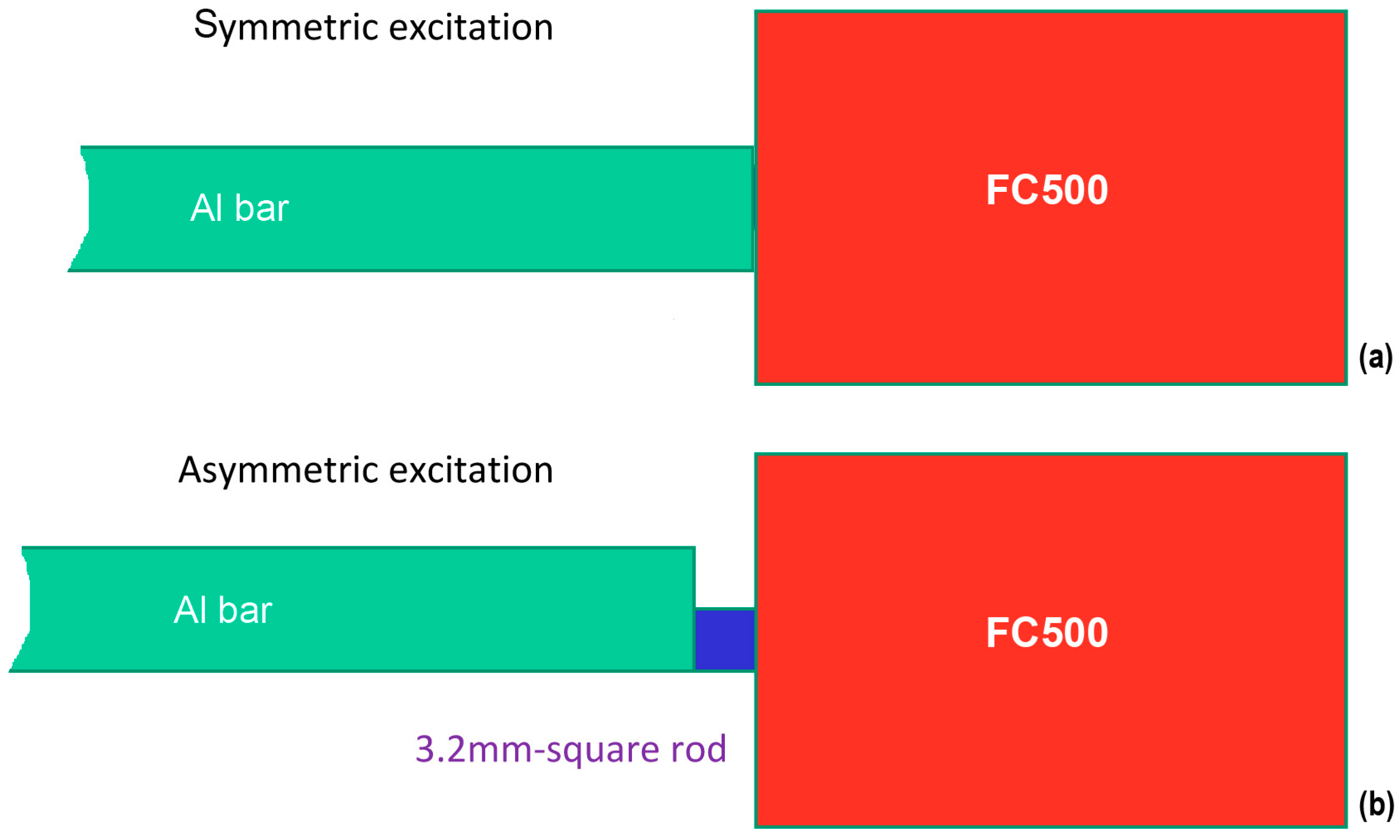
In most of this study, bar waves were produced utilizing a symmetric excitation method. This is shown in the top part of Figure A1. A transmitter (FC500) is glued (using epoxy) at the central position and most of the end surface of the bar was subjected to the displacement pulse from the transmitter. Because of the symmetry, bar-wave modes similar to symmetric plate waves are produced on the test bar. Another approach is to apply the displacement pulse in asymmetric manner. This study used an arrangement shown in the lower part of Figure A1. Here, a square-rod of 3.2 mm was inserted (by epoxy bonding) between the transmitter and the test bar and only one side of the bar is excited, favoring the generation of asymmetric bar-wave modes.
Figure A1.
Bar wave generation utilizing symmetric excitation method (a) and asymmetric excitation method (b).
Figure A1.
Bar wave generation utilizing symmetric excitation method (a) and asymmetric excitation method (b).

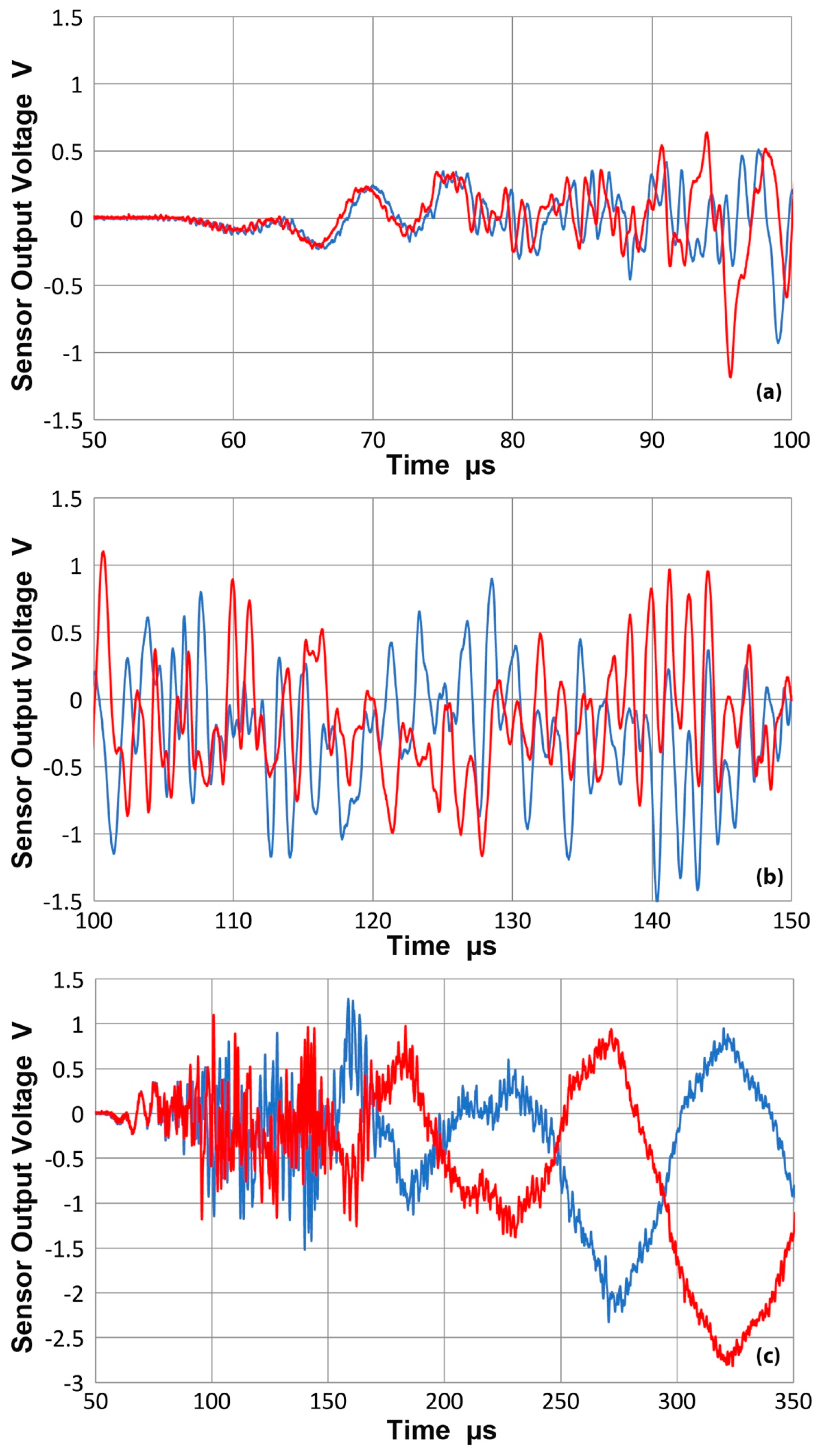
When asymmetric excitation is used, the output waveforms on opposite surfaces showed different trend from that found in Figure 7 with the symmetric excitation, where the wave phases matched well from the initial arrival up to 150 µs. Here, a shorter bar of 1.05 m was used to compare the excitation methods. As Figure A2a shows, the phases started to shift from about 70 µs and asymmetric wave modes became evident at 90 µs or the velocity of 3 mm/µs. Figure A2b covers the period between 90 and 150 µs and in this segment, the two waveforms showed the features of opposite phase or the wave modes to be fully asymmetric. Beyond 150 µs, Figure A2c clearly exhibits asymmetric behavior.
Figure A2.
(a) The received waveforms from asymmetric excitation method on opposite surfaces using a KRN sensor (#11063 with FET buffer) at 300 mm from the transmitter. From 50 to 100 µs. Compare to Figure 7; (b) Same as (a), but for 100 to 150 µs; (c) Same as (a), but for 50 to 350 µs.
Figure A2.
(a) The received waveforms from asymmetric excitation method on opposite surfaces using a KRN sensor (#11063 with FET buffer) at 300 mm from the transmitter. From 50 to 100 µs. Compare to Figure 7; (b) Same as (a), but for 100 to 150 µs; (c) Same as (a), but for 50 to 350 µs.

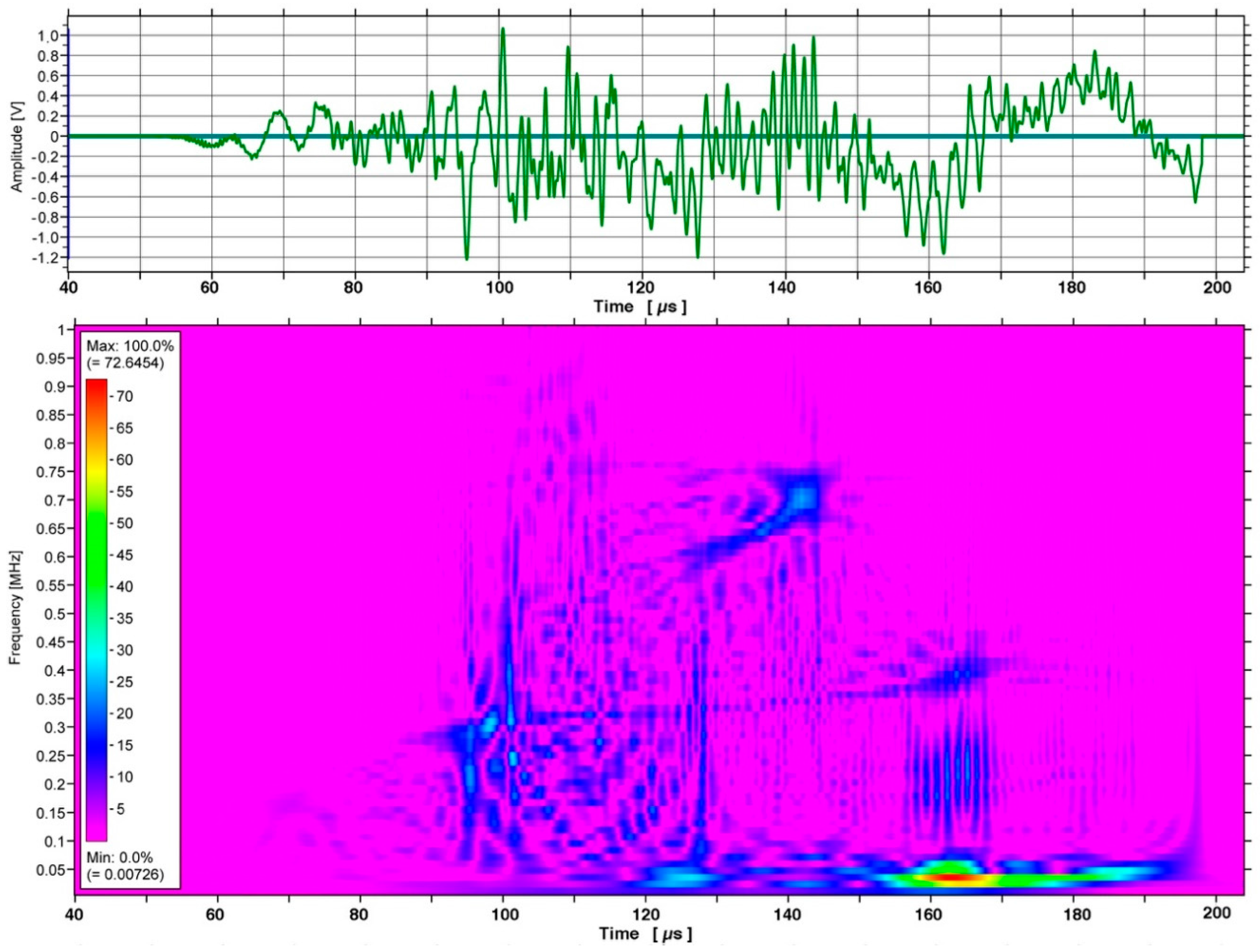
Figure A3 is CWT spectrograms, comparable to Figure 6, except this plot was obtained using the asymmetric excitation method. This figure shows weaker peak intensities at peak positions corresponding to cw1 through cw5. The low frequency (below 100 kHz) peaks are seen, but shifted to later arrival (>150 µs). These are possibly related to x- and y-displacement dominated modes, seen in Figure 5a. A new peak appears at 140 µs and 700 kHz, which was absent in Figure 6. For this position, there are numerous modes indicated in Figure 5a and its origin is indeterminate.
Figure A3.
Output waveform of a KRN sensor (#11063) from asymmetric excitation method and its CWT spectrogram for 40–200 µs segment up to 1 MHz. Compare to Figure 6 from symmetric excitation method.
Figure A3.
Output waveform of a KRN sensor (#11063) from asymmetric excitation method and its CWT spectrogram for 40–200 µs segment up to 1 MHz. Compare to Figure 6 from symmetric excitation method.

Appendix B. KRN Sensors without FET
Two KRN sensors (KRNBB-PCP #12035 and #12060: without an FET buffer) were tested at L = 300 mm with the output termination (or input resistance Rin) of 10 kΩ along with a microdot cable of 60 cm length (C = 72 pF). The input capacitance of the oscilloscope (14 pF) is also in parallel. These have a small diameter of 1 mm sensing area, as in the FET-buffered version. The output waveform (#12035) and its CWT spectrogram are shown in Figure A4. Overall, this resembles Figure 4, but spectral intensities below 100 kHz are absent unlike in Figure 6. This part differs from the corresponding part of FET-buffered KRN sensors discussed earlier.
Figure A4.
Output waveform of a KRN sensor without FET buffer (#12035) from symmetric excitation method and its CWT spectrogram for 40–200 µs segment up to 1 MHz. Notice much lower intensities below 100 kHz in comparison to Figure 6.
Figure A4.
Output waveform of a KRN sensor without FET buffer (#12035) from symmetric excitation method and its CWT spectrogram for 40–200 µs segment up to 1 MHz. Notice much lower intensities below 100 kHz in comparison to Figure 6.

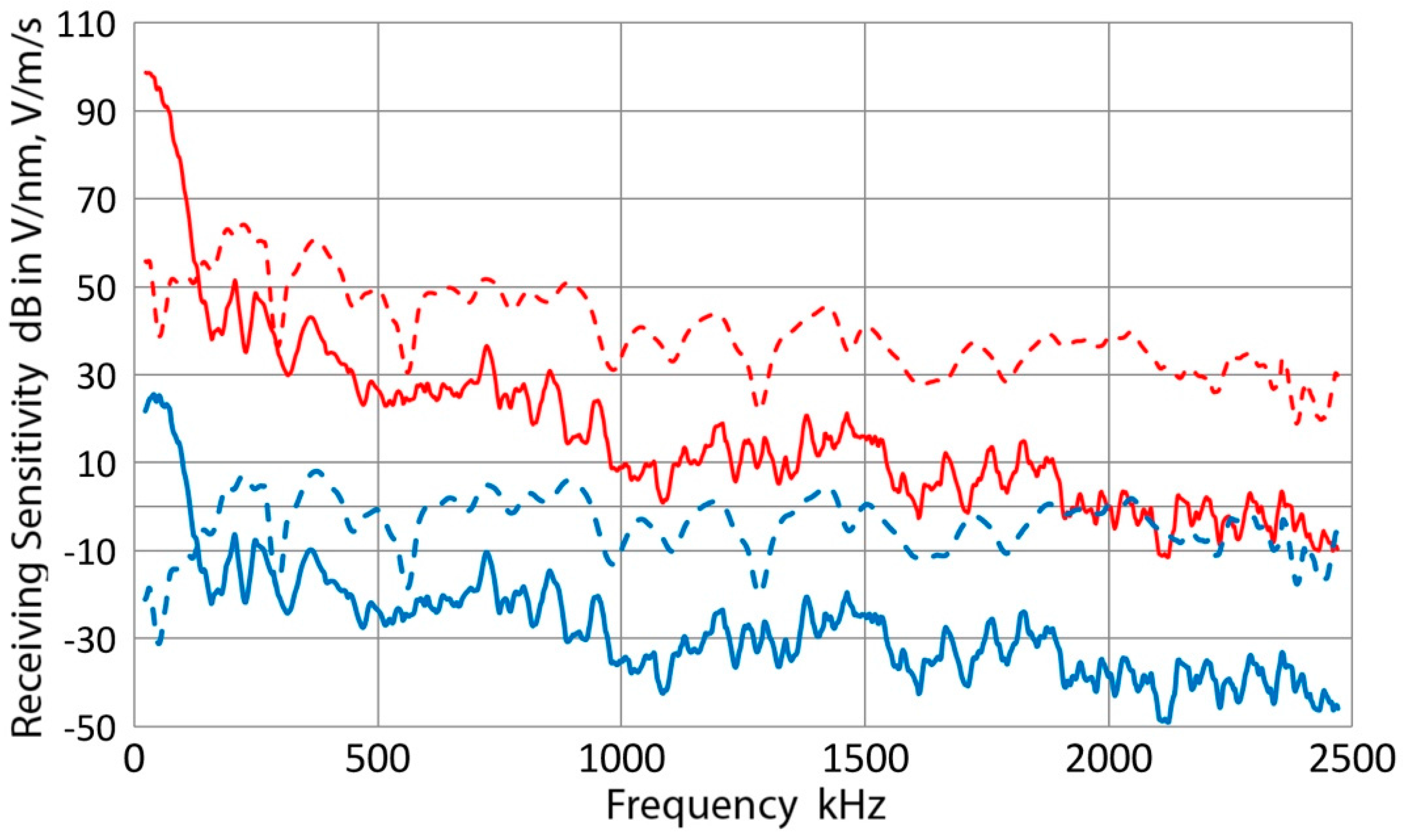
Receiving bar-wave displacement sensitivity was obtained in the same manner as in the main text. Results are given in Figure A5 for #12035. Red curve gives the sensitivity with the same set-up as in Figure A4; that is, with C = 72 + 14 = 86 pF and Rin = 10 kΩ. Blue curve is the data for C = 10 pF and 10 MΩ (with the use of a BK Precision 10× probe) and green curve for C = 86 pF and Rin = 100 kΩ. The blue and green curves are separated by 10 dB, while the green and red curves match above 300 kHz. Below 300 kHz, the red curve had smaller increase of 18 dB in comparison to 30 dB rise observed in the blue and green curves. All three curves were relatively flat from 300 kHz to 1 MHz except for many fluctuations. The sensitivities further decreased at higher frequencies. For the FET-buffered sensors (cf. Figure 8b), comparable sensitivity increases at low frequencies were found and general trends are similar to the cases of high Rin (blue and green curves).
Figure A5.
Displacement sensitivity curves for bar waves of KRN sensor (#12035) without FET buffer: blue curve for Rin = 10 MΩ/C = 10 pF, green curve for Rin = 100 kΩ/C = 86 pF and red for Rin = 10 kΩ/C = 86 pF. Compare to Figure 8b for KRN sensors with FET buffer.
Figure A5.
Displacement sensitivity curves for bar waves of KRN sensor (#12035) without FET buffer: blue curve for Rin = 10 MΩ/C = 10 pF, green curve for Rin = 100 kΩ/C = 86 pF and red for Rin = 10 kΩ/C = 86 pF. Compare to Figure 8b for KRN sensors with FET buffer.

The receiving sensitivities to bar waves (in solid curves) and normally incident waves (in dashed curves) are compared in Figure A6 for #12035. The data was determined with the output termination of 10 kΩ via a coaxial cable (with 72 pF capacitance). In comparison to the corresponding data for the FET-buffered sensors given in Figure 8a, this figure shows general reduction in sensitivities. For the peak values of the blue dash curves, and for the average levels over 300–900 kHz of the blue curves, the differences are about 25 dB. The decrease in the displacement sensitivity below 100 kHz (blue dash) was even higher.
Figure A6.
Receiving sensitivity of a KRN sensor without FET buffer (#12035). The displacement receiving sensitivities are shown in blue curves and velocity sensitivities are in red. Solid lines are for the bar-wave data, while dashed curves are for the sensitivities to normally incident waves. Compare to Figure 8c. Green curve is the high-impedance sensitivity to normally incident waves from reference [4].

Previously, the sensitivity data to normally incident waves was obtained in reference [4], using a 100× probe in order to minimize sensor loading. This corresponded to Rin = 100 MΩ in parallel to 3 pF. The peak value for the high-impedance data was −10 dB (Figure 6c in reference [4]), shown here as green curve. For the FET-buffered sensor, it was 4.7 dB, as was shown in Figure 8a (blue dash curve). This sensitivity difference of 15 dB comes from the amplification effect of the FET. For the blue dash curve of Figure A6, the receiving sensitivity was reduced by 8 to 12 dB by lowering the input resistance to 10-kΩ in parallel to 72 pF. A part of this loss (7.3 dB) was due to the cable capacitance as the sensor capacitance is 40 pF (33 pF for #12060 and the loss is 8.1 dB). Some loss also comes from the reduction of the input impedance, and from the input capacitance of digital oscilloscope (14 pF). Thus, the use of a coaxial cable contributes a 10 dB loss, corresponding to the difference between blue and green curves in Figure A5.
Figure A7 gives CWT spectrogram corresponding to Figure A4, except asymmetrical excitation method was used. There are peaks at cw1 to cw5, but cw6 is absent. Instead, a prominent peak appears at 140 µs and 700 kHz, as was the case for Figure A2. This is the only peak associated with the asymmetrical excitation, although the mode is unknown. The peak at cw3 is much stronger, and it stretched to higher frequency side, to 650 kHz. There was a weak trace in Figure A4 at this position, although its origin is unknown. As noted for Figure A2, many scattered spot intensities were seen. Again, the cause of this behavior needs further work.
Figure A7.
Output waveform of a KRN sensor without FET buffer (#12035) from asymmetric excitation method and its CWT spectrogram for 40–200 µs segment up to 1 MHz. Notice much lower intensities below 100 kHz in comparison to Figure A3.
Figure A7.
Output waveform of a KRN sensor without FET buffer (#12035) from asymmetric excitation method and its CWT spectrogram for 40–200 µs segment up to 1 MHz. Notice much lower intensities below 100 kHz in comparison to Figure A3.

Appendix C. R6a Sensors
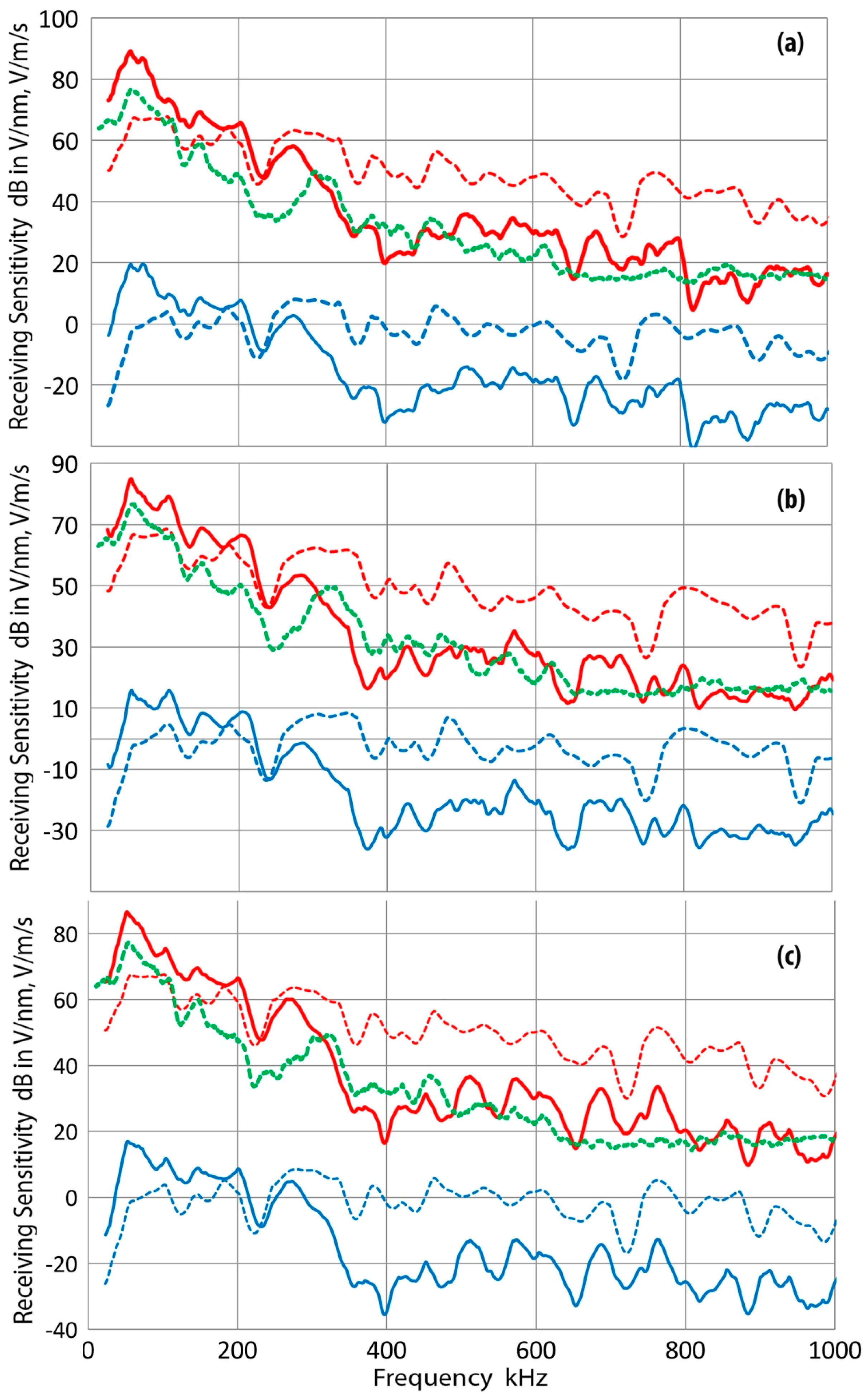
This part provides additional graphical data in support of earlier discussion of the sensor characteristics of R6a. It was shown that the bar-wave velocity sensitivity data provides an adequate representation of the surface-wave velocity sensitivity. Three following figures, Figure A8a–c, are included below to reinforce the conclusion reached earlier in this study.
Figure A8.
Receiving sensitivity of PAC R6a. (a) AI05; (b) AI08; (c) AI09. The displacement receiving sensitivities are shown in blue curves and velocity sensitivities are in red. Solid lines are for the bar-wave data, while dashed curves are for the sensitivities to normally incident waves. Green curve is the velocity calibration for surface waves from PAC.

Appendix D. FET Buffer
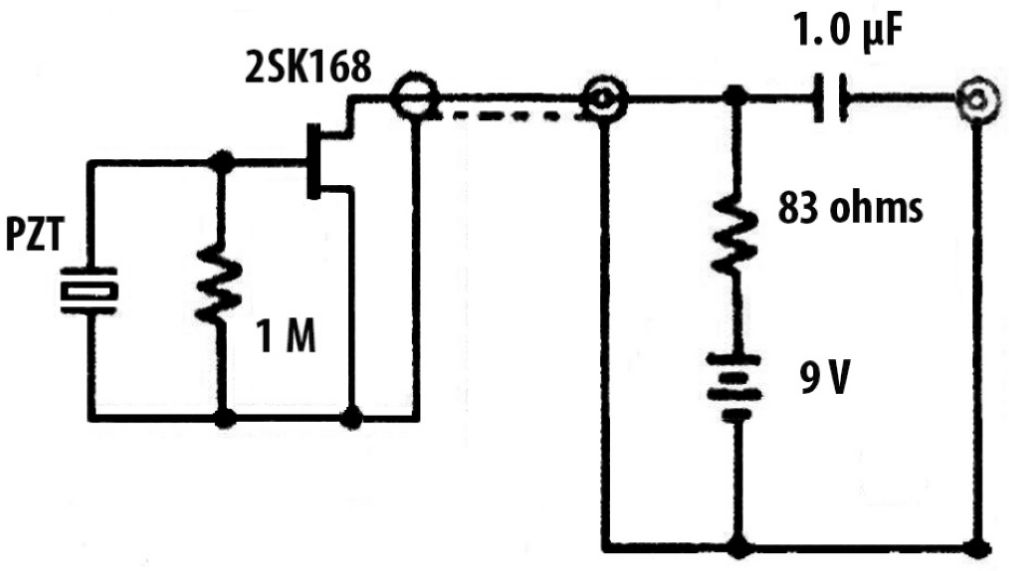
Since Shiwa et al. [19] designed an input buffer circuit with an FET for increasing the sensitivity of a piezoelectric sensing element, such an FET buffer has been used in many other AE sensors. While the internal wirings of commercial sensors have not been disclosed, the circuit is expected to be similar to Figure A9. This drawing is based on Shiwa’s input buffer circuit, in which he used 2SK715, a load resistance of 750 Ω and power supply of 18 V. Here, the actual load resistance of 83 Ω (nominal value = 75 Ω) and 9 V supply voltage were used. This circuit differs from that suggested by DWC for use with their B1080-LD (results were reported in Section 3.2.2). The DWC circuit uses an inductor (3.3 mH used) in lieu of the road resistor in Figure A9 and adds a 75-Ω termination after the dc-blocking capacitor (1 µF).
Figure A9.
Circuit diagram of an FET buffer.

The gain of the FET buffer is expected to change with the load resistance. By using 2SK168 with load resistance values of 83 Ω or 531 Ω (16.1 dB difference), their effects on the output were evaluated. KRN (#12060) sensor was used and placed face-to-face with Olympus V192, driven by monopolar pulse of −130 V peak. With the load resistance of 83 Ω, the peak output of the FET buffer circuit (Figure A9) was 0.433 V, while it was 2.23 V with the load resistance of 531 Ω; an increase of 14.3 dB. An approximate proportionality is observed. (Note that 2SK168 is obsolete. A better choice is 2SK3557, which has the same drain current limit of 50 mA as 2SK715.) Consequently, the use of an FET buffer with a particular power supply can result in different gain for the FET buffer. While the type of FET and internal circuit can also change the net gain, it is concluded that the increased sensitivity levels with FET-buffered KRN sensors, (observed in Section 3.2.1), are due to the gain of the FET buffer, as noted in Appendix B.
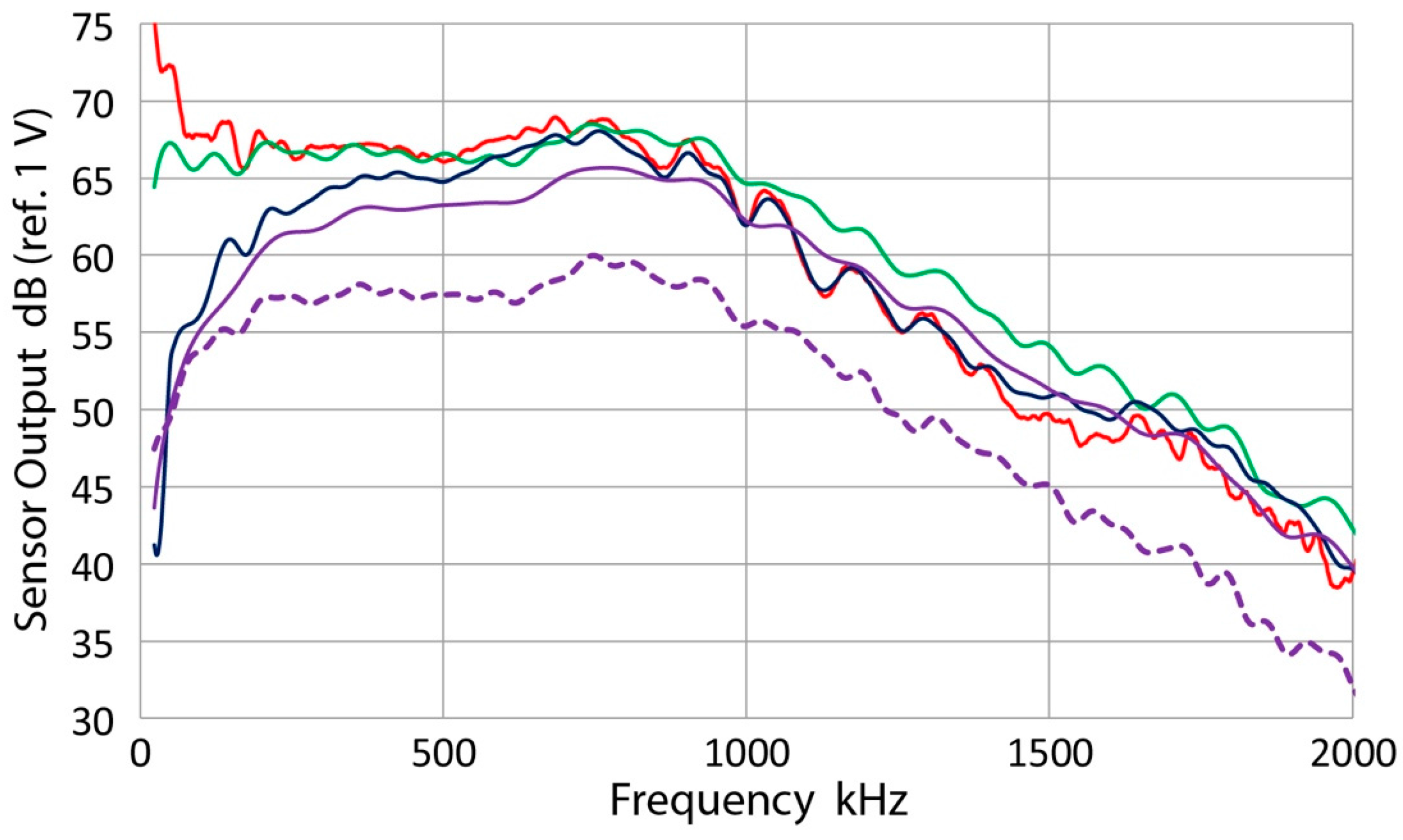
Effects of an FET buffer and the input resistance, Rin, were further examined. The same test set-up as in the preceding paragraph was used. First, with Rin = 1 MΩ, the sensor output was connected to an oscilloscope through an FET buffer (R = 83 Ω). Its output FFT spectrum is given as the red curve in Figure A10. Next, the sensor output was connected directly to the oscilloscope input (Rin = 1 MΩ in parallel to 14 pF) using a 10 cm tinned wire. This minimized the stray capacitance (around 3 pF) and produced the green curve. Note the increased levels below 100 kHz for the red curve, indicating the low-frequency enhancement of 8 dB due to the FET buffer circuit. (The gain of the FET buffer was −1.4 dB and not adjusted.) In the next series, Rin of 10 kΩ was used. Using another FET buffer, the obtained FFT spectrum is given as the blue curve with its peak nearing that of the red curve. However, a sharp drop-off occurred below 400 kHz. Next, the direct connection to the oscilloscope input with 10 kΩ in parallel, giving the purple curve. The shape of this curve is similar to that of the green curve above 500 kHz, but low-frequency drop-off is present. Finally, a coaxial cable was used for connecting the sensor to the oscilloscope with a 10 kΩ termination. This is given as purple dash curve, showing approximately 6 dB below the purple curve above 500 kHz, decreasing as the frequency is reduced and merging to the blue and purple curves below 50 kHz. The low-frequency output reduction is due to the small sensor capacitance (40 pF) and Rin of 10 kΩ, which together form a high-pass filter acting on the voltage generated in the sensor. This effect is especially significant below 150 kHz. Thus, this type of conical element sensors requires at least 100 kΩ input resistance. These results suggest the needs for a calibration source in evaluating sensors and effects of signal conditioning schemes to be used for improved sensing performance.
Figure A10.
Output spectra from KRN sensor (#12060) excited by Olympus V192 using various input parameters. Red: FET buffer with Rin = 1 MΩ, Green: direct oscilloscope input with Rin = 1 MΩ/C = 14 pF, Blue: FET buffer with Rin = 10 kΩ, Purple: direct oscilloscope input with Rin = 100 kΩ/C = 14 pF, Purple dash: cable connection with Rin = 10 kΩ/C = 86 pF.

References
- Miller, R.K.; Hill, E.V. (Eds.) Nondestructive Testing Handbook, Acoustic Emission, 3rd ed.; ASNT: Columbus, OH, USA, 2005; Volume 6, p. 446. [Google Scholar]
- ASTM International. ASTM E1106-12 Standard Method for Primary Calibration of Acoustic Emission Sensors; ASTM International: West Conshohocken, PA, USA, 2016; p. 12. [Google Scholar] [CrossRef]
- ASTM International. ASTM E976-15, Standard Guide for Determining the Reproducibility of Acoustic Emission Sensor Response; ASTM International: West Conshohocken, PA, USA, 2015; p. 7. [Google Scholar]
- Ono, K. Calibration methods of acoustic emission sensors. Materials 2016, 9, 508. [Google Scholar] [CrossRef] [PubMed]
- Ono, K. Critical examination of ultrasonic transducer characteristics and calibration methods. Res. Nondestruct. Eval. 2017, in press. [Google Scholar]
- Hatano, H.; Watanabe, T. Reciprocity calibration of acoustic emission transducers in Rayleigh-wave and longitudinal-wave sound fields. J. Acoust. Soc. Am. 1997, 101, 1450–1455. [Google Scholar] [CrossRef]
- The Japanese Society for Non-Destructive Inspection. NDIS 2109-91, Method for Absolute Calibration of Acoustic Emission Transducers by Reciprocity Technique; ISOTR13115 (2011); The Japanese Society for Non-Destructive Inspection: Tokyo, Japan, 1991. [Google Scholar]
- Ono, K.; Cho, H.; Matsuo, T. New characterization methods of AE sensors. J. Acoust. Emiss. 2010, 28, 256–277. [Google Scholar]
- Hayashi, T.; Song, W.; Rose, J.L. Guided wave dispersion curves for a bar with an arbitrary cross-section, a rod and rail example. Ultrasonics 2003, 41, 175–183. [Google Scholar] [CrossRef]
- Hamstad, M.A.; Gary, J.; O’Gallagher, A. Far-field acoustic emission waves by three-dimensional finite element modeling of pencil-lead breaks on a thick plate. J. Acoust. Emiss. 1996, 14, 103–114. [Google Scholar]
- McLaskey, G.; Glaser, S. Acoustic emission sensor calibration for absolute source measurements. J. Nondestruct. Eval. 2012, 31, 157–168. [Google Scholar] [CrossRef]
- Greenspan, M. The NBS conical transducer: Analysis. J. Acoust. Soc. Am. 1987, 81, 173–183. [Google Scholar] [CrossRef]
- Proctor, T. An improved piezoelectric acoustic emission transducer. J. Acoust. Soc. Am. 1982, 71, 1163–1168. [Google Scholar] [CrossRef]
- Beattie, A.G. Acoustic emission, Principles and instrumentation. J. Acoust. Emiss. 1983, 2, 95–128. [Google Scholar]
- Goujon, L.; Baboux, J.C. Behaviour of acoustic emission sensors using broadband calibration techniques. Meas. Sci. Technol. 2003, 14, 903–908. [Google Scholar] [CrossRef]
- Monnier, T.; Seydou, D.; Godin, N.; Zhang, F. Primary calibration of acoustic emission sensors by the method of reciprocity, theoretical and experimental considerations. J. Acoust. Emiss. 2012, 30, 152–166. [Google Scholar]
- Kim, K.Y.; Castagnede, B.; Sachse, W. Miniaturized capacitive transducer for detection of broadband ultrasonic signals. Rev. Sci. Instrum. 1989, 60, 2785–2788. [Google Scholar] [CrossRef]
- Manthei, G. Characterization of acoustic emission sources in a rock salt specimen under triaxial compression. Bull. Seismol. Soc. Am. 2005, 95, 1674–1700. [Google Scholar] [CrossRef]
- Shiwa, M.; Inaba, H.; Kishi, T. Development of the high sensitivity and low noise integrated acoustic emission sensor. In Progress in Acoustic Emission, V, Proceedings of the 10th IAES, JSNDI, Sendai, Japan, 22–25 October 1990; Japanese Society for Non-Destructive Inspection: Tokyo, Japan, 1990; pp. 605–612. [Google Scholar]
Figure 1.
Bar-wave test set-up. An Al6061 bar of 25.4 mm × 6.4 mm × 3660 mm was shaped as shown with an initial straight segment of 700 mm length. FC500 transmitter was glued to its end.
Figure 1.
Bar-wave test set-up. An Al6061 bar of 25.4 mm × 6.4 mm × 3660 mm was shaped as shown with an initial straight segment of 700 mm length. FC500 transmitter was glued to its end.

Figure 2.
(a) Normal displacement in nm vs. time measured at L = 300 mm at the center of the test bar; (b) Normal displacement in nm vs. time measured at L = 300 mm at 5 mm off-center.
Figure 2.
(a) Normal displacement in nm vs. time measured at L = 300 mm at the center of the test bar; (b) Normal displacement in nm vs. time measured at L = 300 mm at 5 mm off-center.

Figure 3.
(a) FFT magnitude spectrum of normal displacement at L = 300 mm at the center; (b) FFT magnitude spectra of normal displacement at L = 300 mm: Center-blue curve, 1 mm off-center-light green, 2 mm off-center-dark red, 3 mm off-center-dark blue, 5 mm off-center-purple, Average of five curves-red.

Figure 4.
Displacement waveform from Figure 3a and its Choi-Williams transform spectrogram for 40–200 µs segment up to 1 MHz. Some peak positions are marked as cw1 to cw6.
Figure 4.
Displacement waveform from Figure 3a and its Choi-Williams transform spectrogram for 40–200 µs segment up to 1 MHz. Some peak positions are marked as cw1 to cw6.

Figure 5.
(a) Dispersion curves of group velocity vs. frequency for bar waves calculated using Hayashi’s theory and semi-analytical finite-element (SAFE) algorithm [9]. Red points represent the modes dominated by z-direction displacement, blue points those by y-direction displacement and black points those by x-direction displacement. The group velocity of S0-mode plate wave for 6.4 mm-thick Al is drawn in as a black curve; (b) The corresponding phase velocity dispersion curves; (c) The group velocity vs. frequency for bar-wave modes dominated by z-direction displacement. Some peak positions are noted by p1 through p6.


Figure 6.
Output waveform of a KRN sensor (#11063) and its CWT spectrogram for 40–200 µs segment up to 1 MHz. Some peak positions are marked as cw1 to cw6, which correspond to those in Figure 4.
Figure 6.
Output waveform of a KRN sensor (#11063) and its CWT spectrogram for 40–200 µs segment up to 1 MHz. Some peak positions are marked as cw1 to cw6, which correspond to those in Figure 4.

Figure 7.
(a) The received waveforms on opposite surfaces using a KRN sensor (#11063 with FET buffer) at 300 mm from the transmitter. From 50 to 100 µs; (b) Same as (a), but for 100–150 µs; (c) Same as (a), but for 50–350 µs.
Figure 7.
(a) The received waveforms on opposite surfaces using a KRN sensor (#11063 with FET buffer) at 300 mm from the transmitter. From 50 to 100 µs; (b) Same as (a), but for 100–150 µs; (c) Same as (a), but for 50–350 µs.

Figure 8.
(a) Receiving sensitivity of a KRN sensor (#11063). The displacement receiving sensitivities are shown in blue curves and velocity sensitivities are in red. Solid lines are for the bar-wave data, while dashed curves are for the sensitivities to normally incident waves; (b) Displacement sensitivity curves for bar waves of two KRN sensors: blue for #11063 and red for #11053. The latter was shifted 4.4 dB, giving a good match for the two curves; (c) Displacement sensitivity curves for normally incident waves of two KRN sensors: blue for #11063 and red for #11053. The latter was shifted 3.0 dB, giving a good match for the two curves, except above 1.4 MHz.

Figure 9.
Effects of changes in L on the integrated signal intensity with two KRN sensors (#12053 and #12060). Red points: frequency range up to 0.5 MHz, Blue points: to 1 MHz, Green points: to 2 MHz.
Figure 9.
Effects of changes in L on the integrated signal intensity with two KRN sensors (#12053 and #12060). Red points: frequency range up to 0.5 MHz, Blue points: to 1 MHz, Green points: to 2 MHz.

Figure 10.
(a) Receiving sensitivity of Valpey-Fisher Pinducer. The displacement receiving sensitivities are shown in blue curves and velocity sensitivities are in red. Solid lines are for the bar-wave data, while dashed curves are for the sensitivities to normally incident waves; (b) Receiving sensitivity of DWC B1080-LD. The displacement receiving sensitivities are shown in blue curves and velocity sensitivities are in red. Solid lines are for the bar-wave data, while dashed curves are for the sensitivities to normally incident waves.

Figure 11.
Receiving sensitivity of PAC R6a (AI06). The displacement receiving sensitivities are shown in blue curves and velocity sensitivities are in red. Solid lines are for the bar-wave data, while dashed curves are for the sensitivities to normally incident waves. Green curve is the velocity calibration for surface waves from PAC.

Figure 12.
Receiving sensitivity of Olympus V103. The displacement receiving sensitivities to bar waves are shown in blue curve for the present work and in red curve from the old data (reproduced with permission from [8]. Copyright AE Group, 2010). Green curve is the displacement receiving sensitivity to normally incident waves [4].

Figure 13.
Receiving sensitivity of PAC S9220. The displacement receiving sensitivities to bar waves are shown in solid blue curve for the present work and in red curve from the old data [8] (reproduced with permission from [8]. Copyright AE Group, 2010). Green curve is the displacement receiving sensitivity to normally incident waves [4]. The velocity sensitivity corresponding to the solid blue curve is given in dotted blue curve.

Figure 14.
Receiving sensitivity of PAC Pico (3804). The displacement receiving sensitivities to bar waves are shown in solid blue curve for the present work and in red curve from the old data [8] (reproduced with permission from [8]. Copyright AE Group, 2010). Green curve is the displacement receiving sensitivity to normally incident waves [4]. The velocity sensitivity corresponding to the solid blue curve is given in dotted blue curve.

Figure 15.
Receiving sensitivity of PAC WD (AC61). The displacement receiving sensitivities are shown in blue curves and velocity sensitivities are in red. Solid lines are for the bar-wave data, while dashed curves are for the sensitivities to normally incident waves.
Figure 15.
Receiving sensitivity of PAC WD (AC61). The displacement receiving sensitivities are shown in blue curves and velocity sensitivities are in red. Solid lines are for the bar-wave data, while dashed curves are for the sensitivities to normally incident waves.

Figure 16.
Receiving sensitivity of PAC µ30D (94). The displacement receiving sensitivities are shown in blue curves and velocity sensitivities are in red. Solid lines are for the bar-wave data, while dashed curves are for the sensitivities to normally incident waves.
Figure 16.
Receiving sensitivity of PAC µ30D (94). The displacement receiving sensitivities are shown in blue curves and velocity sensitivities are in red. Solid lines are for the bar-wave data, while dashed curves are for the sensitivities to normally incident waves.

Figure 17.
Receiving sensitivity of PAC HD50 (NL91). The displacement receiving sensitivities are shown in blue curves and velocity sensitivities are in red. Solid lines are for the bar-wave data, while dashed curves are for the sensitivities to normally incident waves.
Figure 17.
Receiving sensitivity of PAC HD50 (NL91). The displacement receiving sensitivities are shown in blue curves and velocity sensitivities are in red. Solid lines are for the bar-wave data, while dashed curves are for the sensitivities to normally incident waves.

Figure 18.
Receiving sensitivity of PAC R15 (BS90). The displacement receiving sensitivities to bar waves are shown in solid blue curve for the present work and in red curve from the old data [8]. (reproduced with permission from [8]. Copyright AE Group, 2010). Green curve is the displacement receiving sensitivity to normally incident waves [4]. The velocity sensitivity corresponding to the solid blue curve is given in dotted blue curve.

Figure 19.
Receiving sensitivity of PAC R15a (BD72). The displacement receiving sensitivities are shown in blue curves and velocity sensitivities are in red. Solid lines are for the bar-wave data, while dashed curves are for the sensitivities to normally incident waves. Green curve is the velocity calibration to normally incident waves from PAC (converted from µbar to m/s unit).

Figure 20.
Receiving sensitivity of PAC F30a (AA20). The displacement receiving sensitivity to bar waves is shown in solid blue curve. Green curve is the displacement receiving sensitivity to normally incident waves [4]. The velocity sensitivity corresponding to the solid blue curve is given in dotted blue curve.

Figure 21.
Receiving sensitivity of DECI SH225 (104). The displacement receiving sensitivities are shown in blue curves and velocity sensitivities are in red. Solid lines are for the bar-wave data, while dashed curves are for the sensitivities to normally incident waves.
Figure 21.
Receiving sensitivity of DECI SH225 (104). The displacement receiving sensitivities are shown in blue curves and velocity sensitivities are in red. Solid lines are for the bar-wave data, while dashed curves are for the sensitivities to normally incident waves.

Figure 22.
Receiving sensitivity of Olympus V101. The displacement receiving sensitivity to bar waves is shown in solid blue curve. Green curve is the displacement receiving sensitivity to normally incident waves from reference [4]. The velocity sensitivity corresponding to the solid blue curve is given in dotted blue curve.


Table 1.
Transducers used.
| Transducer Model | Manufacturer | Frequency MHz | Element Size (mm) |
|---|---|---|---|
| FC500 | AET Corp | 2.25 | 19 |
| B1080-LD | Digital Wave | 0.2–1.5 | 3.2 |
| SH-225 | Dunegan Engineering | 0.225 | 6.3 × 12.6 * |
| KRNBB-PCP or -PC | KRN Services | 0.1–1 | 1 |
| V101 | Olympus | 0.5 | 25.4 |
| V103 | Olympus | 1 | 12.7 |
| R6-alpha | Physical Acoustics | 0.06 | 12.7 |
| R15 | Physical Acoustics | 0.15 | 12.7 |
| R15-alpha | Physical Acoustics | 0.15 | 12.7 |
| F30-alpha | Physical Acoustics | 0.2–0.7 | 12.7 ** |
| Pico | Physical Acoustics | 0.5 | 3.2 |
| S9220 | Physical Acoustics | 0.9 | 8 |
| HD-50 | Physical Acoustics | 0.5 | 3 |
| WD | Physical Acoustics | 0.3–0.5 | 12.7 ** |
| µ30D | Physical Acoustics | 0.3 | 8 |
| Pinducer VP-1093 | Valpey-Fisher | 0.1–2 | 1.35 |
* Rectangular shear element; ** Multiple elements.
© 2017 by the authors. Licensee MDPI, Basel, Switzerland. This article is an open access article distributed under the terms and conditions of the Creative Commons Attribution (CC BY) license (http://creativecommons.org/licenses/by/4.0/).
Share and Cite
MDPI and ACS Style
Ono, K.; Hayashi, T.; Cho, H. Bar-Wave Calibration of Acoustic Emission Sensors. Appl. Sci. 2017, 7, 964. https://doi.org/10.3390/app7100964
AMA Style
Ono K, Hayashi T, Cho H. Bar-Wave Calibration of Acoustic Emission Sensors. Applied Sciences. 2017; 7(10):964. https://doi.org/10.3390/app7100964
Chicago/Turabian StyleOno, Kanji, Takahiro Hayashi, and Hideo Cho. 2017. "Bar-Wave Calibration of Acoustic Emission Sensors" Applied Sciences 7, no. 10: 964. https://doi.org/10.3390/app7100964
Note that from the first issue of 2016, this journal uses article numbers instead of page numbers. See further details here.