Large Earthquake Magnitude Prediction in Chile with Imbalanced Classifiers and Ensemble Learning

Abstract

This work presents a novel methodology to predict large magnitude earthquakes with horizon of prediction of five days. For the first time, imbalanced classification techniques are applied in this field by attempting to deal with the infrequent occurrence of such events. So far, classical classifiers were not able to properly mine these kind of datasets and, for this reason, most of the methods reported in the literature were only focused on moderate magnitude prediction. As an additional step, outputs from different algorithms are combined by applying ensemble learning. Since false positives are quite undesirable in this field, due to the social impact that they might cause, ensembles have been designed in order to reduce these situations. The methodology has been tested on different cities of Chile, showing very promising results in terms of accuracy.

1. Introduction

As the magnitude of an earthquake increases, its destructiveness also does. The need to predict an earthquake is particularly relevant when its magnitude is large. About one million earthquakes of magnitude $M_s=2.0$ occur annually across the world. However, there are only seven recorded earthquakes with a magnitude equal to or greater than 9. The low frequency with which large-scale earthquakes occur is an added difficulty for the study of their prediction, as modeled in Gutenberg-Richter law.

In machine learning, this problem is widely known as imbalanced classification. A dataset is imbalanced when there exists one class with one label to which the majority of instances belong to (typically 70% or higher). Alternatively, a small number of instances are assigned to the other label (minority), usually the one with higher interest [1]. When the dataset exhibits such data distribution, standard classification algorithms, which search for a global performance, are not able to accurately predict instances with minority presence in the dataset. That is, they tend to assign minority instances to the label containing the majority of instances.

In the case at hand, the minority label is related to the occurrence of large magnitude earthquakes and the goal is to predict if an earthquake of large magnitude will occur during the next five days. In order to manage this problem, it is proposed a novel methodology based on algorithms specialized in imbalanced learning. To carry out this methodology, datasets that collect the seismic activity of several cities in Chile have been used. Furthermore, ensemble learning has been applied in order to make more accurate predictions [2], as a result of combining the strengths of the different imbalanced classifiers here analyzed.

The remainder of the paper is structured as follows. The state-of-the-art is reviewed in Section 2, in which both general-purpose imbalanced classifiers and approaches particularly designed for earthquake prediction are discussed. Section 3 describes the proposed methodology, including the algorithms evaluated and the ensembles generated. Results for different zones in Chile are reported in Section 4. Finally, the conclusions drawn from this study are summarized in Section 5.

2. Related Works

The problem of earthquake prediction, especially big magnitude ones, has generated a great number of approaches, from many different points of view [3].

Alimoradi and Beck [4] presented a method of data-based probabilistic seismic hazard analysis (PSHA) and ground motion simulation, verified using previously recorded strong-motion data and machine-learning techniques. It showed the benefits of applying such methods to strong-motion databases for PSHA and ground motion simulation, particularly in large urban areas, where dense instrumentation is available or expected.

The use of artificial neural networks (ANNs) has been extensively proposed in recent years [5]. In particular, the authors in [6] estimated the magnitude of the events recorded daily, showing as the ANNs are a promising technique for earthquake prediction. It is also proved that ANN training on the global data on earthquakes is much more effective for a local earthquake prediction, than an ANN training on local data.

Other approaches, like [7], focus on preparing data-sets. In this case, a monitoring system to prepare machine learning data-sets for earthquake prediction based on seismic-acoustic signals is proposed due to the difficulty of making predictions given that kind of data. Using on-line recordings of robust noise monitoring (RNM) signals of anomalous seismic processes (ASP) from stations in Azerbaijan, an Earthquake-Well Signal Monitoring Software has been developed to construct data sets.

Another promising approach for the next generation of earthquake early warning system is based on predicting ground motion directly from observed ground motion, without any information of hypocenter. Ogiso et al. [8] predicted seismic intensity at the target stations from the observed ground motion at adjacent stations, employing two different methods of correction for site amplification factors: scalar correction and frequency-dependent correction prediction, being this last one more accurate. Frequency-dependent correction for site amplification in the time domain may lead to more accurate prediction of ground motion in real time.

Multi-step prediction is also present in literature. The authors in [9] proposed a multi-step prediction method of EMD-ELM (empirical mode decomposition-extreme learning machine) to achieve the short-term prediction of strong earthquake ground motions. The predicted results of near-fault acceleration records demonstrate that the EMD-ELM method can realize multi-step prediction of acceleration records with relatively high accuracy.

Bayesian networks (BNs) were used as a novel methodology in order to analyze the relationships among the earthquake events in [10]. The authors proposed a way to predict earthquake from a new perspective, constructing a BN after processing, which is derived from the earthquake network based on space-time influence domain. Then, the BN parameters are learnt by using the cases which are designed from the seismic data in the period between 1992 and 2012. At last, predictions are done for the data in the period between 2012 and 2015, combining the BN with the parameters. The results show that the success rate of the prediction including delayed prediction is about 65%.

In the context of the imbalanced learning, there are several approaches that have been recently published addressing different problems. Li et al. [11] presented a method for identifying peptide motifs binding to 14-3-3$\sigma$ isoform, in which a similarity-based undersampling approach and a SMOTE-like oversampling approach are used to deal with imbalanced distribution of the known peptide motifs, contributing to create a fast and reliable computational method that can be used in peptide-protein binding identification in proteomics research.

In [12] an optimization model using different swarm strategies (Bat-inspired algorithm and PSO) is proposed for adaptively balancing the increase/decrease of the class distribution, depending on the properties of the biological datasets, which pretends to achieving the highest possible accuracy and Kappa statistics as well. Tested on five imbalanced medical datasets, that are sourced from lung surgery logs and virtual screening of bioassay data, results show that the proposed optimization model outperforms other class balancing methods in medical data classification.

New re-sampling methods also appear in recent literature. A new oversampling method called Cluster-based Weighted Oversampling for Ordinal Regression (CWOS-Ord) is proposed in [13] for addressing ordinal regression with imbalanced datasets. It aims to address this problem by first clustering minority classes and then oversampling them based on their distances and ordering relationship to other classes’ instances. Results demonstrate that the proposed CWOS-Ord method provides significantly better results compared to other methods based on the performance measures.

Another algorithm, K Rare-class Nearest Neighbour (KRNN) is proposed in [14], by directly adjusting the induction bias of the k Nearest Neighbours (KNN). First, dynamic query neighbourhoods are formed, and to further adjust the positive posterior probability estimation to bias classification towards the rare class. Results showed that KRNN significantly improved KNN for classification of the rare class, and often outperformed re-sampling and cost-sensitive learning strategies with generality-oriented base learners.

The occurrence of a minority class has also been forecasted by means of imbalanced classifiers, in the field of electricity [15]. The authors used different imbalanced approaches, combined with certain resampling methods, to forecast outliers in data from Spain’s electricity demand. Reported results confirmed the usefulness of their approach.

Imbalanced learning is present too on diagnosis of bearings, which generally plays an important role in fault diagnosis of mechanical system. An online sequential prediction method for imbalanced fault diagnosis problem based on extreme learning machine is proposed in [16], where under-sampling and over-sampling techniques plays again an important role. Using two typical bearing fault diagnosis data, results demonstrate that the proposed method can improve the fault diagnosis accuracy with better effectiveness and robustness than other algorithms.

Moreover, there are other approaches that applied imbalanced techniques to different data types, like images [17,18], which involve high dimensional data resulting on robustness methods to address class imbalance.

In conclusion, imbalanced learning has been widely studied in the literature, particularly in biology and clinical datasets. Additionally, a vast majority of approaches for earthquake prediction are focused on events of moderate magnitude. But the use of imbalanced classification for predicting large earthquakes is not reported in the state-of-the-art. It is then justified the need and novelty of using these techniques in this research field.

3. Methodology

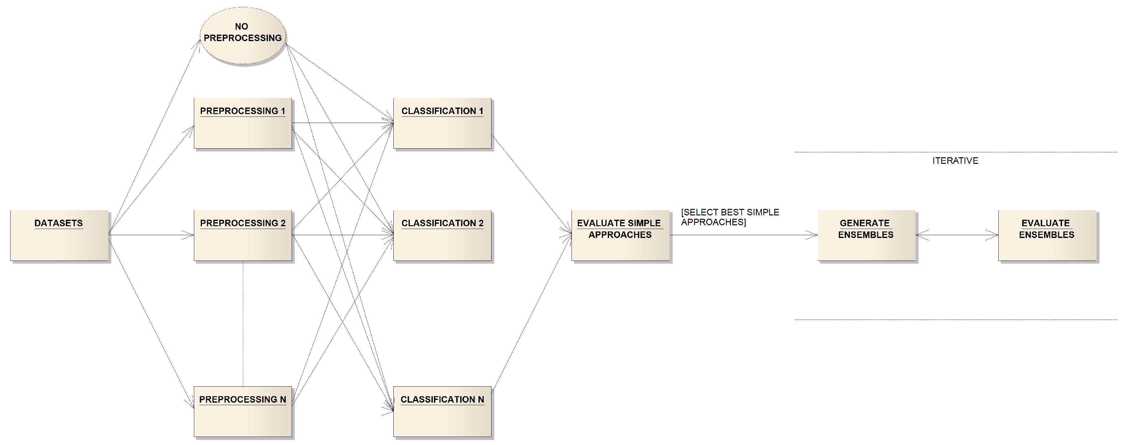
The methodology designed is carried out as follows: given a dataset, this is rebalanced by applying a preprocessing algorithm. Then, a classification algorithm is applied to the rebalanced dataset in order to obtain an accurate result. In this methodology, all the classifiers created in this first stage are named as simple classifiers since they are created by using only one classification algorithm and one (or none) preprocessing algorithm. This is only a nomenclature, since it is possible that some classification algorithms used internally contain some preprocessing. Figure 1 illustrates the general procedure.

As a first stage, the goal is to obtain as many simple classifiers as possible combinations between preprocessing and classification algorithms exist.

The approaches proposed to solve imbalanced classification problems can be split into two differentiated groups: algorithm-based approaches that design specific algorithms to deal with the minority class, and data-based approaches, which apply a preprocessing step to try to balance the classes before applying a learning algorithm [2]. In this work, a selection of representative methods of the first group are firstly used, and thereafter, the algorithm with the best performance will be combined with different preprocessing methods in order to improve the results of the predictions.

Table 1. Techniques of imbalanced classification.

Preprocessing			Classification
Algorithm	Type	Reference	Algorithm	Reference
ADASYN	Oversampling	[20]	AdaBoost	[21]
ADOMS	Oversampling	[22]	AdaBoostM1	[23]
ROS	Oversampling	[24]	AdaBoostM2	[25]
Safe-Level-Smote	Oversampling	[26]	Bagging	[27]
SMOTE	Oversampling	[28]	BalanceCascade	[29]
SMOTE-ENN	Oversampling	[24]	C45CS	[30]
SMOTE-TL	Oversampling	[24]	C-SVMCS	[31]
SPIDER	Oversampling	[32]	DataBoost-IM	[33]
SPIDER2	Oversampling	[26]	EasyEnsemble	[29]
CNN	Undersampling	[34]	UnderBagging	[35]
CNNTL	Undersampling	[36]	UnderBagging2	[35]
TL	Undersampling	[36]	UnderOverBagging	[37]

shows both preprocessing and classification techniques that have been used. Due to the good behavior exhibited in oversampling methods [2], a number of oversampling-based preprocessing techniques greater than that ones based on undersampling has been tested. All these techniques can be found in the KEEL open source java software project [19].

Once all simple classifiers are created and evaluated, the best of them are selected so as to be used in the second stage, where ensembles are generated. The selection criterion of the best simple classifiers of a dataset consists in selecting the 15 classifiers with the highest Area Under the ROC Curve (AUC) as long as these conditions are satisfied:

• The AUC is greater than 0.6 in order to avoid selecting bad classifiers that could hinder the generation of good ensembles. In case of having less than 15 classifiers with an AUC greater than 0.6, select only those fulfilling this criterion.
• There are not selected classifiers with equal AUC in order to avoid selecting identical classifiers that would generate redundant ensembles. In case of having two or more classifiers with equal AUC, randomly select only one of them and continue selecting the next classifiers with the highest AUC.

After having selected the best simple classifiers, the methodology generates the ensembles in the second stage of the methodology so as to obtain classifiers which could improve the performance of the simple classifiers.

Ensembles are developed to combine several classifiers’ outputs. In this sense, they can be designed for two different purposes: (1) to increase sensitivity (2) to increase specificity. If option (1) is desired then an OR ensemble is the most suitable one, since an “1” is predicted if at least one classifier predicts an “1”. By contrast, if option (2) is desired then an AND ensemble must be applied. Given the nature of the problem, the second option has been chosen for this work.

These ensembles are the result of the intersection between the predictions of the simple classifiers which intervene in the generation of them. The intersection of different predictions reduces the number of false positives, that is, avoids to predict that a large earthquake will occur for the next five days and it does not really occur. Obviously, a decrease of the large earthquakes properly predicted by the classification technique is also expected (a sensitivity reduction) but, as discussed in [38], triggering a false alarm is quite an undesirable situation.

Table 2. Illustrative example of the proposed ensemble, in order to reduce false positives.

Model 1	Model 2	Model 3	Ensemble
0	0	0	0
0	0	1	0
0	1	0	0
0	1	1	0
1	0	0	0
1	0	1	0
1	1	0	0
1	1	1	1

illustrates an example about how the prediction is made when three models are considered. Only if all the three models agree in assigning a “1” to the sample to be classified, “1” is assigned. In this case, “1” would mean that a large earthquake will occur for the next five days.

The ensembles generation is done in an iterative way. First, all ensembles from two simple classifiers are generated; then, three simple classifiers are used to generate the ensembles and so until either all existing ensembles from simple classifiers selected in the previous stage are generated or an tensemble whose performance meets expectations it is found.

During the generation of ensembles, if the probability of correctly predicting a large earthquake is equal to one for an ensemble then new ensembles are not generated from this one. Thus, generating useless classifiers whose performance do not improve the best classifier found so far is avoided. It can be noted that the main consequence of computing the final forecasting by using the intersection of the predictions between some classifiers is to create more conservative classifiers with less false positives and a higher probability of correctly predicting large earthquakes, in exchange of a less number of large earthquakes properly predicted. Therefore, if an ensemble is generated from another ensemble that predicts correctly large earthquakes with a probability of one, there is no room for improvement and it is not possible to find a new ensemble that reduces the number of false positives and increases this probability, making useless this generation.

After generating, evaluating and selecting the best ensembles, the methodology is concluded. The flowchart describing the full methodology in shown in Figure 2.

4. Results

This section reports all the achieved results, after application of the proposed methodology to different Chilean datasets. First, the quality parameters used to assess the performance of the method are described in Section 4.1. Second, Section 4.2 describes how data have been preprocessed and generated, in order to efficiently process imbalanced datasets or, in other words, to process datasets containing large earthquakes. Then, Section 4.3, Section 4.4 and Section 4.5 discuss the results obtained for the cities of Santiago, Valparaíso and Talca, respectively.

4.1. Quality Parameters to Assess the Model

This section briefly summarizes the parameters used to assess the performance of the method. First, it is defined what true positives (TP), true negatives (TN), false positives (FP) and false negatives (FN) mean in the context of earthquake prediction:

(1)

TP. The methodology predicts that a large earthquake is occurring within the next five days and it does occur.

(2)

TN. The methodology predicts that a large earthquake is not occurring within the next five days and it does not occur.

(3)

FP. The methodology predicts that a large earthquake is occurring within the next five days but it does not occur.

(4)

FN. The methodology predicts that a large earthquake is not occurring within the next five days but it does occur.

From all these statistics, several well-known measures can be calculated. In particular, sensitivity ($S_n$), specificity ($S_p$), positive predictive value (PPV), negative predictive values (NPV), F-measure or balanced F-score (F), Matthew’s correlation coefficient (MCC), geometric mean (GM) and AUC. Their formulas are listed below:

$$\begin{array}{ccc}\hfill S_n& =& \frac{TP}{TP+FN}\hfill \end{array}$$

(1)

$$\begin{array}{ccc}\hfill S_p& =& \frac{TN}{TN+FP}\hfill \end{array}$$

(2)

$$\begin{array}{ccc}\hfill PPV& =& \frac{TP}{TP+FP}\hfill \end{array}$$

(3)

$$\begin{array}{ccc}\hfill NPV& =& \frac{TN}{TN+FN}\hfill \end{array}$$

(4)

$$\begin{array}{ccc}\hfill F& =& \frac{2·PPV·S_n}{S_n+PPV}\hfill \end{array}$$

(5)

$$\begin{array}{ccc}\hfill MCC& =& \frac{TP\times TN-FP\times FN}{\sqrt{(TN+FN)(TP+FP)(TP+FN)(TN+FP)}}\hfill \end{array}$$

(6)

$$\begin{array}{ccc}\hfill GM& =& \sqrt{S_n·S_p}\hfill \end{array}$$

(7)

$$\begin{array}{ccc}\hfill AUC& =& \frac{1+S_n+FP/size\left(Dataset\right)}{2}\hfill \end{array}$$

(8)

4.2. Datasets Description and Generation

The target zones are those introduced in [38]. In it, the authors studied four regions in Chile: Santiago, Valparaíso, Talca and Pichilemu. However, before applying the methodology to all datasets, they must be analyzed in order to select only those which could be useful for the application of imbalanced classifiers. Note that the class indicates whether an earthquake with magnitude larger than a preset threshold is occurring within the next five days (label “1”) or not (label “0”). In the original work, the authors set this threshold so that datasets were not imbalanced.

Therefore, first of all and for every dataset, it is shown in

Table 3. Imbalance ratio for all datasets initially considered.

Datasets	Total	Positives	Negatives	Imbalance
Pichilemu_M4	343	211	132	61.52%
Pichilemu_M5	343	122	221	35.57%
Pichilemu_M6	343	8	335	2.33%
Pichilemu_M7	343	6	337	1.75%
Talca_M4	204	69	135	33.82%
Talca_M5	204	7	197	3.43%
Talca_M6	204	0	204	0
Talca_M7	204	0	204	0
Santiago_M4	480	21	459	4.38%
Santiago_M5	480	0	480	0
Santiago_M6	480	0	480	0
Santiago_M7	480	0	480	0
Valparaíso_M4	979	166	813	16.96%
Valparaíso_M5	979	42	937	4.29%
Valparaíso_M6	979	0	979	0
Valparaíso_M7	979	0	979	0

the total number of cases, as well as positive and negative cases from each one of them. Besides, it is shown the ratio of positive cases over total cases, which determines how imbalanced the dataset is. $Mx$, with $x=4,5,6,7$ means that the class has been assigned considering magnitudes greater than x. For instance, Pichilemu_M4 indicates data from the region of Pichilemu, with binary classes showing magnitudes larger than 4.0.

Second, some datasets are discarded. In particular, all datasets without positive cases are discarded. Additionally, all datasets which are not imbalanced (positive cases <15%) are discarded as well.

As the evaluation technique used is the standard holdout, with 66% of cases in training set and 34% of cases in test set, it is shown in

Table 4. Positive and negative cases distribution in training and test sets with 66–34%.

City	Training (66%)			Test (34%)
	Total	Positives	Negatives	Total	Positives	Negatives
Pichilemu_M6	228	8	220	115	0	115
Pichilemu_M7	228	6	222	115	0	115
Talca_M5	136	7	129	68	0	68
Santiago_M4	320	9	311	160	12	148
Valparaíso_M5	652	7	645	327	35	292

how positive and negative cases are distributed in training and test sets, respectively, for every dataset.

All datasets without positive cases in the test set are discarded, remaining only two datasets to which the proposed methodology can be applied (Santiago_M4 and Valparaíso_M5). In order to use some of the discarded datasets and enlarge the experimentation, it is shown in

Table 5. Positive and negative cases distribution in training and test sets with 50–50%.

City	Training (50%)			Test (50%)
	Total	Positives	Negatives	Total	Positives	Negatives
Pichilemu_M6	172	8	164	171	0	171
Pichilemu_M7	172	6	166	171	0	171
Talca_M5	102	2	100	102	5	97

how positive and negative cases would be distributed if an alternative holdout (50% of cases in training set and 50% of cases in test set) would be used on all those discarded datasets.

Considering this new distribution, one of the three previously discarded datasets can be eventually used (Talca_M5). Finally,

Table 6. Selected datasets with size for training and test sets.

City	M4	M5	M6	M7
Pichilemu	–	–	–	–
Santiago	66–34%	–	–	–
Talca	–	50–50%	–	–
Valparaíso	–	66–34%	–	–

shows the selected datasets and which evaluation technique has been used for each one.

Please note that all processed datasets will be available upon acceptance.

4.3. Santiago M4

Table 7. Fifteen imbalanced classifiers with Area Under the ROC Curve (AUC) > 0.6 in Santiago.

Index	Preprocessing	Classifier	TP	FP	TN	FN	${\mathit{S}}_{\mathit{n}}$	${\mathit{S}}_{\mathit{p}}$	PPV	NPV	F	AUC	MCC	GM
1	SMOTE	NNCS	12	57	91	0	1	0.62	0.17	1	0.53	0.81	0.33	0.78
2	OSS	OverBagging	8	23	125	4	0.67	0.85	0.26	0.97	0.64	0.76	0.34	0.75
3	SMOTE_TL	NNCS	10	51	97	2	0.83	0.66	0.16	0.98	0.53	0.74	0.27	0.74
4	Safe_Level_SMOTE	NNCS	11	67	81	1	0.92	0.55	0.14	0.99	0.47	0.73	0.24	0.71
5	OSS	OverBagging2	8	33	115	4	0.67	0.78	0.20	0.97	0.58	0.72	0.27	0.72
6	OSS	SMOTEBagging	8	34	114	4	0.67	0.77	0.19	0.97	0.58	0.72	0.26	0.72
7	OSS	UnderOverBagging	8	35	113	4	0.67	0.74	0.19	0.97	0.57	0.72	0.26	0.71
8	None	NNCS	12	91	57	0	1	0.39	0.12	1	0.38	0.69	0.21	0.62
9	CPM	OverBagging2	8	46	102	4	0.67	0.69	0.15	0.96	0.52	0.68	0.20	0.68
10	SPIDER2	UnderBagging	7	35	113	5	0.58	0.76	0.17	0.96	0.55	0.67	0.21	0.67
11	CNNTL	OverBagging2	9	63	85	3	0.75	0.58	0.13	0.97	0.47	0.66	0.17	0.66
12	CNN	UnderBagging2	7	39	109	5	0.58	0.74	0.15	0.96	0.54	0.66	0.19	0.66
13	None	BalanceCascade	9	64	84	3	0.75	0.57	0.12	0.97	0.46	0.66	0.17	0.65
14	OSS	RUSBoost	12	102	46	0	1	0.31	0.11	1	0.33	0.66	0.18	0.56
15	AHC	EasyEnsemble	6	30	118	6	0.50	0.80	0.17	0.95	0.56	0.65	0.19	0.63
Average			9	51.33	96.67	3	0.75	0.65	0.16	0.97	0.51	0.70	0.23	0.68

shows the fifteen selected classifiers that satisfy the selection criterion (combination of preprocessing and classifier algorithms with AUC greater than 0.6).

It stands out that the NNCS and the Bagging classifiers are present in almost all selected simple classifiers, and OSS in preprocessing algorithms. Nevertheless, these classifiers show a very low PPV. Therefore, the need of accomplishing the next step, ensembles generation, is justified. Ensembles with better metrics are shown in

Table 8. Ensembles generated for Santiago.

Ensemble	TP	FP	TN	FN	${\mathit{S}}_{\mathit{n}}$	${\mathit{S}}_{\mathit{p}}$	PPV	NPV	F	AUC	MCC	GM
4, 5, 7, 8, 10, 11, 12, 14, 15	5	2	146	7	0.42	0.99	0.71	0.95	0.75	0.70	0.52	0.64
1, 4, 8, 10, 11, 14, 15	6	3	145	6	0.50	0.98	0.67	0.96	0.77	0.74	0.55	0.70
2, 4, 5, 7, 8, 11, 12, 14, 15	5	3	145	7	0.42	0.98	0.63	0.95	0.73	0.70	0.48	0.64
2, 4, 5, 7, 8, 10, 11, 12, 14	6	4	144	6	0.50	0.97	0.60	0.96	0.76	0.74	0.52	0.70
Average	5.50	3	145	6.50	0.46	0.98	0.65	0.96	0.75	0.72	0.52	0.67

.

It can be seen that PPV and $S_p$ have improved markedly compared to simple classifiers, reaching values greater than 0.7 for the best ensemble. Global measures like F-Value and MCC have experimented a good improvement as well. Actually, average values for these parameters are above 0.7 and 0.5, respectively. In contrast, $S_n$ has worsened (as expected) and GM is slightly lower (0.67 vs. 0.68), but still satisfactory.

4.4. Valparaíso M5

In this case, only seven simple classifiers have an AUC higher than 0.6. Such algorithms are shown in

Table 9. Seven imbalanced classifiers with AUC $>0.6$ in Valparaíso.

Index	Preprocessing	Classifier	TP	FP	TN	FN	${\mathit{S}}_{\mathit{n}}$	${\mathit{S}}_{\mathit{p}}$	PPV	NPV	F	AUC	MCC	GM
1	CNN	UnderBagging	27	107	185	8	0.77	0.63	0.2	0.96	0.54	0.70	0.25	0.70
2	CNN	EasyEnsemble	30	151	141	5	0.86	0.48	0.17	0.97	0.46	0.67	0.21	0.64
3	SMOTE	NNCS	30	155	137	5	0.86	0.47	0.16	0.96	0.45	0.66	0.20	0.63
4	Safe Level	NNCS	29	151	141	6	0.83	0.48	0.16	0.96	0.46	0.66	0.19	0.63
5	CNNTL	BalanceCascade	32	177	115	3	0.91	0.39	0.15	0.97	0.41	0.65	0.20	0.60
6	Borderline	NNCS	25	142	150	10	0.71	0.51	0.15	0.94	0.46	0.61	0.14	0.61
7	TL	NNCS	26	157	135	9	0.74	0.46	0.14	0.94	0.43	0.60	0.13	0.59
Average			28.43	148.57	143.43	6.57	0.81	0.49	0.16	0.96	0.46	0.65	0.19	0.63

.

NNCS algorithm is present in 4 out of the 7 selected classifiers. In general, $S_p$ is low and PPV is very low. Best generated ensembles are shown in

Table 10. Ensembles generated for Valparaíso.

Ensemble	TP	FP	TN	FN	${\mathit{S}}_{\mathit{n}}$	${\mathit{S}}_{\mathit{p}}$	PPV	NPV	F	AUC	MCC	GM
1, 2, 3, 4, 6	17	29	263	18	0.48	0.90	0.37	0.94	0.67	0.69	0.34	0.66
1, 2, 3, 4, 5, 6	16	28	264	19	0.46	0.90	0.36	0.93	0.66	0.68	0.33	0.64
1, 3, 4, 6	18	32	260	17	0.51	0.89	0.36	0.94	0.67	0.70	0.35	0.68
1, 2, 3, 5, 6	19	34	258	16	0.54	0.88	0.36	0.94	0.67	0.71	0.36	0.69
1, 3, 4, 5, 6	17	31	261	18	0.49	0.89	0.35	0.94	0.66	0.69	0.33	0.66
1, 2, 3, 6	20	37	255	15	0.57	0.87	0.35	0.94	0.67	0.72	0.36	0.71
1, 2, 4, 6	17	32	260	18	0.49	0.89	0.35	0.94	0.66	0.69	0.33	0.66
1, 3, 6	21	40	252	14	0.60	0.86	0.34	0.95	0.67	0.73	0.37	0.72
Average	18.13	32.88	259.13	16.88	0.52	0.89	0.36	0.94	0.67	0.70	0.35	0.68

.

PPV and $S_p$, measures which are very low in simple classifiers, have improved in the ensembles (almost 100% and 150% improvement, respectively). Global measures are better in general too, being MCC the one with higher improvement (from 0.19 to 0.35). Only $S_n$ has worsened, which was an expected behavior due to the restrictive nature of the ensembles generated. Although the ensembles have improved the simple classifiers, PPV must still be improved for this dataset. Current 0.36 is much better than former 0.16 but it is still somewhat low.

4.5. Talca M5

Table 11. Fifteen imbalanced classifiers with AUC $>0.6$ in Talca.

Index	Preprocessing	Classifier	TP	FP	TN	FN	${\mathit{S}}_{\mathit{n}}$	${\mathit{S}}_{\mathit{p}}$	PPV	NPV	F	AUC	MCC	GM
1	ADASYN	NNCS	5	7	93	0	1	0.93	0.42	1	0.78	0.97	0.62	0.96
2	CPM	C45CS	5	19	81	0	1	0.81	0.21	1	0.62	0.90	0.41	0.90
3	ADASYN	Bagging	5	21	79	0	1	0.79	0.19	1	0.60	0.89	0.39	0.89
4	ADASYN	UnderOverBagging	5	23	77	0	1	0.77	0.18	1	0.59	0.88	0.37	0.88
5	ADASYN	OverBagging	5	23	77	0	1	0.77	0.18	1	0.59	0.88	0.37	0.88
6	SPIDER2	NNCS	4	15	85	1	1	0.85	0.21	0.99	0.62	0.82	0.36	0.83
7	CPM	NNCS	4	18	82	1	1	0.82	0.18	0.99	0.60	0.81	0.32	0.81
8	SMOTE-TL	EasyEnsemble	4	24	76	1	1	0.76	0.14	0.99	0.55	0.78	0.27	0.78
9	NCL	UnderBagging	3	5	95	2	1	0.95	0.38	0.98	0.71	0.78	0.44	0.76
10	SMOTE	BalanceCascade	3	6	94	2	1	0.94	0.33	0.98	0.69	0.77	0.41	0.75
11	Borderline-SMOTE	UnderBagging2	3	7	93	2	1	0.93	0.30	0.98	0.68	0.77	0.39	0.75
12	NCL	Bagging	3	8	92	2	1	0.92	0.27	0.98	0.66	0.76	0.36	0.74
13	TL	NNCS	5	49	51	0	1	0.51	0.09	1	0.42	0.75	0.22	0.71
14	RUS	BalanceCascade	3	11	89	2	1	0.89	0.21	0.98	0.62	0.74	0.31	0.73
15	CPM	AdaBoost	3	12	88	2	1	0.88	0.20	0.98	0.61	0.74	0.29	0.73
Average			4	16.53	83.47	1	1	0.83	0.23	0.99	0.62	0.82	0.37	0.81

shows the fifteen selected classifiers following the selection criterion described in Section 3. Overall, simple classifiers obtained quite good measures, except for PPV, which is a critical measure in the matter at hand. This is due to the high FP/TP rate reached.

Once simple classifiers with good performance are identified (AUC $>0.6$), ensembles composed of two simple classifiers are generated. It has been found that some ensembles reported no FP nor FN. Obviously, this fact leads to perfect values for all the considered quality measures, and therefore, new ensembles with a bigger number of simple classifiers have not been generated. These results are shown in

Table 12. Ensembles generated for Talca.

Ensemble	TP	FP	TN	FN	${\mathit{S}}_{\mathit{n}}$	${\mathit{S}}_{\mathit{p}}$	PPV	PPV	F	AUC	MCC	GM
1, 2	5	0	100	0	1	1	1	1	1	1	1	1
2, 3	5	0	100	0	1	1	1	1	1	1	1	1
2, 4	5	0	100	0	1	1	1	1	1	1	1	1
2, 5	5	0	100	0	1	1	1	1	1	1	1	1
2, 8	4	0	100	1	0.80	1	1	0.99	0.95	0.94	0.89	0.90
1, 9	3	0	100	2	0.60	1	1	0.98	0.90	0.87	0.77	0.78
Average	4.5	0	100	0.5	0.9	1	1	0.99	0.98	0.97	0.96	0.95

. In short, although simple classifiers exhibited good performances, they are not considered reliable enough classifiers because of their low PPV. Ensembles generation have solved this problem, reaching perfect classification with some ensembles.

5. Conclusions

Large magnitude earthquake prediction has been addressed in this work by means of imbalanced classifiers and ensemble learning. As a case study, four cities of Chile (Santiago, Valparaíso, Talca and Pichilemu) have been analyzed, and new imbalanced datasets have been created, using as target label if a large earthquake is occurring or not within the next five days. During the generation of the new datasets, it was found that data from Pichilemu could not be used and, therefore, its study has not been done. Achieved results show meaningful improvement in the three remaining cities when compared to previous works, especially in terms of specificity and PPV. The main limitation of the study carried out is the size of the datasets used, being highly desired to use catalogs with longer historical data for further analysis. Future work is directed towards the generalization of the method, whose promising performance has been reported, by its application across different seismic zones of the world.