Class-Wise Classifier Design Capable of Continual Learning Using Adaptive Resonance Theory-Based Topological Clustering

Abstract

This paper proposes a supervised classification algorithm capable of continual learning by utilizing an Adaptive Resonance Theory (ART)-based growing self-organizing clustering algorithm. The ART-based clustering algorithm is theoretically capable of continual learning, and the proposed algorithm independently applies it to each class of training data for generating classifiers. Whenever an additional training data set from a new class is given, a new ART-based clustering will be defined in a different learning space. Thanks to the above-mentioned features, the proposed algorithm realizes continual learning capability. Simulation experiments showed that the proposed algorithm has superior classification performance compared with state-of-the-art clustering-based classification algorithms capable of continual learning.

1. Introduction

With the recent development of IoT technology, a wide variety of big data from different domains has become easily available. Many studies have proposed machine learning algorithms for classification and clustering to learn useful features/information from the data.

One of the major challenges in the field of machine learning is to achieve continual learning like the human brain using computational algorithms. In general, it is difficult for many computational algorithms to avoid catastrophic forgetting, i.e., previously learned features/information is collapsed due to learning new ones [1], which makes it difficult for the algorithms to realize efficient learning from big data with increasing amounts and types of data. Recently, therefore, computational algorithms capable of continual learning have attracted much attention as a promising approach for continually and efficiently learning useful features/information from big data [2].

Continual learning is categorized into three scenarios: domain incremental learning, task incremental learning, and class incremental learning [3,4]. This paper focuses on class incremental learning, which includes the common real-world problem of incrementally learning new classes of information. In the case of layer-wise neural networks capable of continual learning, their memory capacity is often limited because most of the network architecture is fixed [5]. One promising approach to overcome the limitation of memory capacity is to apply a growing self-organizing clustering algorithm as a classifier. The Self-Organizing Incremental Neural Network (SOINN) [6] is a well-known growing self-organizing clustering algorithm which is inspired by Growing Neural Gas (GNG) [7]. Several conventional studies have shown that SOINN-based classifiers capable of continual learning have good classification performance [8,9,10]. However, the self-organizing process of SOINN-based algorithms is highly unstable due to the instability of GNG-based algorithms.

This paper proposes a new classification algorithm capable of continual learning by utilizing a growing self-organizing clustering based on Adaptive Resonance Theory (ART) [11]. Among recent ART-based clustering algorithms, an algorithm that utilizes Correntropy-Induced Metric (CIM) [12] as a similarity measure shows faster and more stable self-organizing performance than GNG-based algorithms [13,14,15]. We apply CIM-based ART with Edge and Age (CAEA) [16] as a base clustering algorithm in the proposed algorithm. Moreover, we also propose two variants of the proposed algorithm by modifying a computation of the CIM to improve the classification performance. It is expected that the proposed algorithms can utilize large amounts of data more efficiently than conventional algorithms by continually generating classifiers with high classification performance.

The contributions of this paper are summarized as follows:

(i)

A new classification algorithm capable of continual learning, called CAEA Classifier (CAEAC), is proposed by applying an ART-based clustering algorithm. CAEAC generates a new clustering space to learn a new classifier each time a new class of data is given. In addition, thanks to the ART-based clustering algorithm, CAEAC realizes fast and stable computation while avoiding catastrophic forgetting in each clustering space.

(ii)

Two variants of CAEAC, namely CAEAC-Individual (CAEAC-I) and CAEAC- Clustering (CAEAC-C) are introduced to improve the classification performance of CAEAC. These variants use a modified version of the CIM computation (see Section 3.4 in detail).

(iii)

Empirical studies show that CAEAC and its variants have superior classification performance to state-of-the-art clustering-based classifiers.

(iv)

The parameter sensitivity of CAEAC (and its variants) is analyzed in detail.

The paper is organized as follows. Section 2 presents a review of the literature on growing self-organizing clustering algorithms and classification algorithms capable of continual learning. Section 3 describes the details of mathematical backgrounds for CAEAC and its variants. Section 4 presents extensive simulation experiments to evaluate the classification performance of CAEAC and its variants by using real-world datasets. Section 5 concludes this paper.

2. Literature Review

2.1. Growing Self-Organizing Clustering Algorithms

In general, the major drawback of classical clustering algorithms such as the Gaussian Mixture Model (GMM) [17] and k-means [18] is that the number of clusters/partitions has to be specified in advance. GNG [7] and ASOINN [8] are typical types of growing self-organizing clustering algorithms that can handle the drawback of GMM and k-means. GNG and ASOINN adaptively generate topological networks by generating nodes and edges for representing sequentially given data. However, since these algorithms permanently insert new nodes into topological networks for learning useful features/information, they have the potential to forget learned features/information (i.e., catastrophic forgetting). More generally, this phenomenon is called the plasticity-stability dilemma [19]. As a SOINN-based algorithm, SOINN+ [20] can detect clusters of arbitrary shapes in noisy data streams without any predefined parameters. Grow When Required (GWR) [21] is a GNG-based algorithm that can avoid the plasticity-stability dilemma by adding nodes whenever the state of the current network does not sufficiently match to the data. One problem of GWR is that as the number of nodes in the network increases, the cost of calculating a threshold for each node increases, and thus the learning efficiency decreases.

In contrast to GNG-based algorithms, ART-based algorithms can theoretically avoid the plasticity-stability dilemma by utilizing a predefined similarity threshold (i.e., a vigilance parameter) for controlling a learning process. Thanks to this ability, a number of ART-based algorithms and their improvements have been proposed for both supervised learning [22,23,24] and unsupervised learning [25,26,27,28]. Specifically, algorithms that utilize the CIM as a similarity measure have achieved faster and more stable self-organizing performance than GNG-based algorithms [14,15,29,30]. One drawback of the ART-based algorithms is the specification of data-dependent parameters such as a similarity threshold. Several studies have proposed solving this drawback by utilizing multiple vigilance levels [31], adjusting parameters during a learning process [24], and estimating parameters from given data [16]. In particular, CAEA [16], which utilizes the CIM as a similarity measure, has shown superior clustering performance while successfully reducing the effect of data-dependent parameters.

2.2. Classification Algorithms Capable of Continual Learning

In general, continual learning is categorized into three scenarios [3,4]: domain incremental learning [32,33], task incremental learning [34], and class incremental learning [5,34,35,36]. In the deep learning domain, several approaches have been proposed to handle the above scenarios. A regularization-based approach selectively regularizes the variation in network parameters to preserve the important parameters of previously learned tasks [37,38]. A replay-based approach maintains the performance of trained tasks by storing selected training samples in a limited memory buffer and using them when training new tasks [39,40,41,42]. Although there are several approaches for continual learning, the ability of neural networks to perform continual learning without catastrophic forgetting is still not sufficient [43]. The major problem with the above approaches is that the structure of networks is basically fixed, and therefore, there is an upper limit on the memory capacity.

One promising approach to overcome this difficulty caused by the fixed network structure is to apply a growing self-organizing clustering algorithm as a classifier. The growing self-organizing clustering algorithms adaptively and continually generate a node to represent new information. Typical classifiers of this type are the Episodic-GWR [44] and ASOINN classifiers (ASC) [8], which utilize GWR and ASOINN, respectively. One state-of-the-art algorithm is SOINN+ with ghost nodes (GSOINN+) [10]. GSOINN+ has successfully improved the classification performance by generating some ghost nodes near a decision boundary of each class.

Another successful approach is ART-based supervised learning algorithms, i.e., ARTMAP [22,23,24,26,29,45]. As mentioned in Section 2.1, ART-based algorithms theoretically realize sequential and class-incremental learning without catastrophic forgetting. However, especially for an algorithm with an ARTMAP architecture, label information is not fully utilized during a supervised learning process. In general, a class label of each node is determined based on the frequency of the label appearance. Therefore, there is a possibility that a decision boundary of each class cannot be learned clearly.

3. Proposed Algorithm

In this section, first, the overview of CAEAC is introduced. Next, the mathematical backgrounds of the CIM and CAEA are explained in detail. Then, modifications of the CIM computation are introduced for variants of CAEAC.

Table 1. Summary of notations.

Notation	Description
$\mathcal{X}=$$\{{\mathbf{x}}_1,{\mathbf{x}}_2,\dots ,{\mathbf{x}}_n,\dots \}$	A set of training data points
${\mathbf{x}}_n=$$\left(x_{n1},x_{n2},\dots ,x_{nd}\right)$	d-dimensional training data point (the nth data point)
C	The number of classes in $\mathcal{X}$
${\mathcal{X}}_c$	A set of training data points belongs to the class $c\in C$
$\mathcal{Y}=\{{\mathbf{y}}_1,{\mathbf{y}}_2,\dots ,{\mathbf{y}}_K\}$	A set of prototype nodes
${\mathbf{y}}_k=$$\left(y_{k1},y_{k2},\dots ,y_{kd}\right)$	d-dimensional prototype node (the kth node)
$\mathcal{S}=\{{\sigma }_1,{\sigma }_2,\dots ,{\sigma }_K\}$	A set of bandwidths for a kernel function
${\kappa }_{\sigma }$	Kernel function with a bandwidth $\sigma$
CIM	Correntropy-Induced Metric
$k_1$, $k_2$	Indexes of the 1st and 2nd winner nodes
${\mathbf{y}}_{k_1}$, ${\mathbf{y}}_{k_2}$	The 1st and 2nd winner nodes
$V_{k_1}$, $V_{k_2}$	Similarities between a data point ${\mathbf{x}}_n$ and winner nodes (${\mathbf{y}}_{k_1}$ and ${\mathbf{y}}_{k_2}$)
$V_{\mathrm{threshold}}$	Similarity threshold (a vigilance parameter)
${\mathcal{N}}_{k_1}$	A set of neighbor nodes of node ${\mathbf{y}}_{k_1}$
${\alpha }_{k_1}$	The number of data points that have accumulated by the node ${\mathbf{y}}_{k_1}$
$\lambda$	Predefined interval for computing $\sigma$ and deleting an isolated node
$e_{\left(k_1,k_2\right)}$	Edge connection between nodes ${\mathbf{y}}_{k_1}$ and ${\mathbf{y}}_{k_2}$
$a_{(k_1,k_2)}$	Age of edge $e_{\left(k_1,k_2\right)}$
$a_{\max }$	Predefined threshold of an age of edge

summarizes the main notations used in this paper.

3.1. Class-Wise Classifier Design Capable of Continual Learning

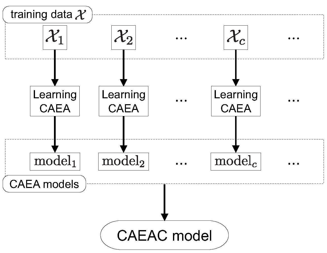
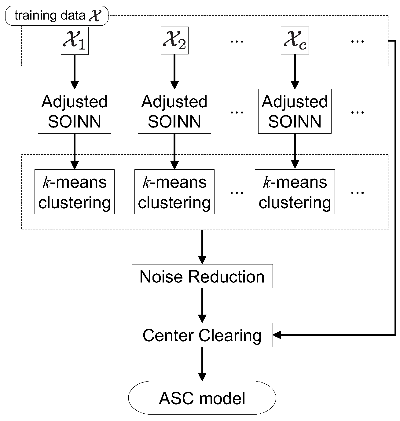
Figure 1 shows the overview of CAEAC. The architecture of CAEAC is inspired by ASC [8]. As shown in Figure 2, ASC is an ASOINN-based supervised classifier incorporating k-means and two node clearance mechanisms after class-wise unsupervised self-organizing processes. The main difference between CAEAC and ASC is that CAEAC does not require k-means and node clearance mechanisms because CAEA has superior clustering performance to ASOINN.

In CAEAC, a training dataset is divided into multiple subsets based on their class labels. The number of the subsets is the same as the number of classes. Each subset is used to generate a classifier (i.e., nodes and edges) through a self-organization process by CAEA. Since CAEA is capable of continual learning, each classifier can be continually updated. Moreover, when a training dataset belongs to a new class, a self-organizing space of CAEA is newly defined. Thus, it is possible to learn new features/information without destroying existing one. When classifying an unknown data point, classifiers (one classifier for each class) are installed in the same space, and the label information of the nearest neighbor node of the unknown data point is output as a classification result. The learning procedure of CAEAC is summarized in Algorithm 1.

Algorithm 1: Learning Algorithm of CAEAC

   In the following subsections, the mathematical backgrounds of the CIM and CAEA are explained in detail.

3.2. Correntropy and Correntropy-Induced Metric

Correntropy [12] provides a generalized similarity measure between two arbitrary data points $\mathbf{x}=(x_1,x_2,\dots ,x_d)$ and $\mathbf{y}=(y_1,y_2,\dots ,y_d)$ as follows:

$$C(\mathbf{x},\mathbf{y})=\mathbf{E}\left[{\kappa }_{\sigma }\left(\mathbf{x},\mathbf{y}\right)\right],$$

(1)

where $\mathbf{E}\left[·\right]$ is the expectation operation, and ${\kappa }_{\sigma }\left(·\right)$ denotes a positive definite kernel with a bandwidth $\sigma$. The correntropy is estimated as follows:

$$\widehat{C}(\mathbf{x},\mathbf{y},\sigma )=\frac{1}{d}\sum _{i=1}^d{\kappa }_{\sigma }\left(x_i,y_i\right).$$

(2)

In this paper, we use the following Gaussian kernel in the correntropy:

$${\kappa }_{\sigma }\left(x_i,y_i\right)=exp\left[-\frac{{\left(x_i-y_i\right)}^2}{2{\sigma }^2}\right].$$

(3)

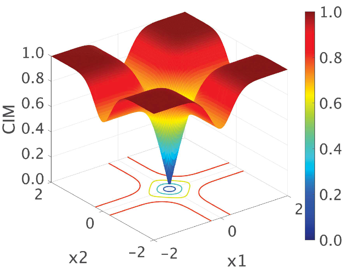
A nonlinear metric called CIM is derived from the correntropy [12]. CIM quantifies the similarity between two data points $\mathbf{x}$ and $\mathbf{y}$ as follows:

$$\mathrm{CIM}\left(\mathbf{x},\mathbf{y},\sigma \right)={\left[1-\widehat{C}(\mathbf{x},\mathbf{y},\sigma )\right]}^{\frac{1}{2}},$$

(4)

where, since the Gaussian kernel in (3) does not have the coefficient $\frac{1}{\sqrt{2\pi }\sigma }$, the range of CIM is limited to $\left[0,1\right]$.

In general, the Euclidean distance suffers from the curse of dimensionality. However, CIM reduces this drawback since the correntropy calculates the similarity between two data points by using a kernel function. Moreover, it has also been shown that CIM with the Gaussian kernel has a high outlier rejection ability [12].

Figure 3 shows the landscape of CIM for the case in which $\mathbf{x}={[x_1,x_2]}^{\top }$ and $\mathbf{y}={[0,0]}^{\top }$.

3.3. CIM-Based ART with Edge and Age

CAEA [16] is an ART-based topological clustering algorithm capable of continual learning. In [16], CAEA and its hierarchical approach show comparable clustering performance to recently-proposed clustering algorithms without the difficulty of parameter specifications to each dataset. The learning procedure of CAEA is divided into four parts: (1) initialization process for nodes and a bandwidth of a kernel function in the CIM, (2) winner node selection, (3) vigilance test, and (4) node learning and edge construction. Each of them is explained in the following subsections.

In this paper, we use the following notations: A set of training data points is $\mathcal{X}=$$\{{\mathbf{x}}_1,{\mathbf{x}}_2,\dots ,{\mathbf{x}}_n,\dots \},$ where ${\mathbf{x}}_n=$$(x_{n1},x_{n2},\dots ,$$x_{nd})$ is a d-dimensional feature vector. A set of prototype nodes in CAEA at the time of the presentation of a data point ${\mathbf{x}}_n$ is $\mathcal{Y}=\{{\mathbf{y}}_1,{\mathbf{y}}_2,$$\dots ,{\mathbf{y}}_K\}$ ($K\in {\mathbb{Z}}^{+}$), where a node ${\mathbf{y}}_k=$$\left(y_{k1},y_{k2},\dots ,y_{kd}\right)$ has the same dimension as ${\mathbf{x}}_n$. Furthermore, each node ${\mathbf{y}}_k$ has an individual bandwidth ${\sigma }_k$ for the CIM, i.e., $\mathcal{S}=\{{\sigma }_1,{\sigma }_2,\dots ,{\sigma }_K\}$.

3.3.1. Initialization Process for Nodes and a Bandwidth of a Kernel Function in the CIM

In the case that CAEA does not have any nodes, i.e., a set of prototype node $\mathcal{Y}=⌀$, the first $(\lambda /2)$th training data points ${\mathcal{X}}_{\mathrm{init}}=\{{\mathbf{x}}_1,{\mathbf{x}}_2,\dots {\mathbf{x}}_{\lambda /2}\}$ directly become prototype nodes, i.e., ${\mathcal{Y}}_{\mathrm{init}}=\{{\mathbf{y}}_1,{\mathbf{y}}_2,\dots ,{\mathbf{y}}_{\lambda /2}\}$, where ${\mathbf{y}}_k={\mathbf{x}}_k$$(k=1,2,\dots ,\lambda /2)$ and $\lambda \in {\mathbb{Z}}^{+}$ is a predefined parameter of CAEA. This parameter is also used for a node deletion process that is explained in Section 3.3.4.

In an ART-based clustering algorithm, a vigilance parameter (i.e., a similarity threshold) plays an important role in a self-organizing process. Typically, the similarity threshold is data-dependent and specified by hand. On the other hand, CAEA uses the minimum pairwise CIM value between each pair of nodes in ${\mathcal{Y}}_{\mathrm{init}}=\{{\mathbf{y}}_1,{\mathbf{y}}_2,\dots ,{\mathbf{y}}_{\lambda /2}\}$, and the average of pairwise CIM values is used as the similarity threshold $V_{\mathrm{threshold}}$, i.e.,

$$V_{\mathrm{threshold}}=\frac{1}{\lambda /2}\sum _{i=1}^{\lambda /2}\underset{j\ne i}{min}\left[\mathrm{CIM}\left({\mathbf{y}}_i,{\mathbf{y}}_j,\sigma \right)\right],$$

(5)

where $\sigma$ is a kernel bandwidth in the CIM.

In general, the bandwidth of a kernel function can be estimated from $\lambda$ instances belonging to a certain distribution [46], which is defined as follows:

$$\mathsf{\Sigma }=U\left(F_{\nu }\right)\mathsf{\Gamma }{\lambda }^{-\frac{1}{2\nu +d}},$$

(6)

$$U\left(F_{\nu }\right)={\left(\frac{{\pi }^{d/2}{2}^{d+\nu -1}{(\nu !)}^{2}R{\left(F\right)}^d}{\nu {\kappa }_{\nu }^2\left(F\right)\left[\left(2\nu \right)!!+(d-1){(\nu !!)}^2\right]}\right)}^{\frac{1}{2\nu +d}},$$

(7)

where $\mathsf{\Gamma }$ denotes a rescale operator (d-dimensional vector), which is defined by a standard deviation of each of the d attributes among $\lambda$ instances, $\nu$ is the order of a kernel, the single factorial of $\nu$ is calculated by the product of integer numbers from 1 to $\nu$, the double factorial notation is defined as $\left(2\nu \right)!!=(2\nu -1)·5·3·1$ (commonly known as the odd factorial), $R\left(F\right)$ is a roughness function, and ${\kappa }_{\nu }\left(F\right)$ is the moment of a kernel. The details of the derivation of (6) and (7) can be found in [46].

In this paper, we use the Gaussian kernel for CIM. Therefore, $\nu =2$, $R\left(F\right)={\left(2\sqrt{\pi }\right)}^{-1}$, and ${\kappa }_{\nu }^2\left(F\right)=1$. Then, (7) is rewritten as follows:

$$\mathbf{H}={\left(\frac{4}{2+d}\right)}^{\frac{1}{4+d}}\mathsf{\Gamma }{\lambda }^{-\frac{1}{4+d}}.$$

(8)

Equation (8) is known as Silverman’s rule [47]. Here, $\mathbf{H}$ contains the bandwidth of a kernel function in CIM. In (8), $\mathsf{\Sigma }$ contains the bandwidth of each attribute (i.e., $\mathsf{\Sigma }$ is a d-dimensional vector). In this paper, the median of the d elements of $\mathsf{\Sigma }$ is selected as a representative bandwidth of the Gaussian kernel in the CIM, i.e.,

$$\sigma =\mathrm{median}\left(\mathsf{\Sigma }\right).$$

(9)

In CAEA, the initial prototype nodes ${\mathcal{Y}}_{\mathrm{init}}=\{{\mathbf{y}}_1,{\mathbf{y}}_2,\dots ,$${\mathbf{y}}_{\lambda /2}\}$ have a common bandwidth of the Gaussian kernel in the CIM, i.e., ${\mathcal{S}}_{\mathrm{init}}=\{{\sigma }_1,{\sigma }_2,\dots ,{\sigma }_{\lambda /2}\}$ where ${\sigma }_1={\sigma }_2=\cdots ={\sigma }_{\lambda /2}$. When a new node ${\mathbf{y}}_{K+1}$ is generated from ${\mathbf{x}}_n$, a bandwidth ${\sigma }_{K+1}$ is estimated from the past $\lambda /2$ data points, i.e., $\{{\mathbf{x}}_{n-\lambda /2},\dots ,{\mathbf{x}}_{n-2},{\mathbf{x}}_{n-1}\}$ by using (6) and (7). As a result, each new node has a different bandwidth $\sigma$ depending on the distribution of training data points. In addition, a set of counters $\mathcal{M}=\{M_1,M_2,\dots ,M_{\lambda /2}\},$ where $M_1=M_2=\cdots =M_{\lambda /2}=1$, is defined. Although the similarity threshold $V_{\mathrm{threshold}}$ depends on the distribution of the initial $\lambda /2$ training data points, we regard that an adaptive $V_{\mathrm{threshold}}$ estimation is realized by assigning a different bandwidth $\sigma$, which affects the CIM value, to each node in response to the changes in the data distribution.

3.3.2. Winner Node Selection

Once a data point ${\mathbf{x}}_n$ is presented to CAEA with the prototype node set $\mathcal{Y}=\{{\mathbf{y}}_1,{\mathbf{y}}_2,\dots ,$${\mathbf{y}}_K\}$, two nodes that have a similar state to the data point ${\mathbf{x}}_n$ are selected, namely, winner nodes ${\mathbf{y}}_{k_1}$ and ${\mathbf{y}}_{k_2}$. The winner nodes are determined based on the state of the CIM as follows:

$$k_1=\underset{{\mathbf{y}}_i\in \mathcal{Y}}{\arg \min }\left[\mathrm{CIM}\left({\mathbf{x}}_n,{\mathbf{y}}_i,\mathrm{mean}\left(\mathcal{S}\right)\right)\right],$$

(10)

$$k_2=\underset{{\mathbf{y}}_i\in \mathcal{Y}\setminus \left\{{\mathbf{y}}_{k_1}\right\}}{\arg \min }\left[\mathrm{CIM}\left({\mathbf{x}}_n,{\mathbf{y}}_i,\mathrm{mean}\left(\mathcal{S}\right)\right)\right],$$

(11)

where $k_1$ and $k_2$ denote the indexes of the 1st and 2nd winner nodes, i.e., ${\mathbf{y}}_{k_1}$ and ${\mathbf{y}}_{k_2}$, respectively. $\mathcal{S}$ is the bandwidths of the Gaussian kernel in the CIM for each node.

3.3.3. Vigilance Test

Similarities between the data point ${\mathbf{x}}_n$ and the 1st and 2nd winner nodes are defined as follows:

$$V_{k_1}=\mathrm{CIM}\left({\mathbf{x}}_n,{\mathbf{y}}_{k_1},\mathrm{mean}\left(\mathcal{S}\right)\right),$$

(12)

$$V_{k_2}=\mathrm{CIM}\left({\mathbf{x}}_n,{\mathbf{y}}_{k_2},\mathrm{mean}\left(\mathcal{S}\right)\right).$$

(13)

The vigilance test classifies the relationship between a data point and a node into three cases by using a predefined similarity threshold $V_{\mathrm{threshold}}$, i.e.,

• Case I

The similarity between the data point ${\mathbf{x}}_n$ and the 1st winner node ${\mathbf{y}}_{k_1}$ is larger (i.e., less similar) than $V_{\mathrm{threshold}}$, namely:

$$V_{\mathrm{threshold}}<V_{k_1}\le V_{k_2}.$$

(14)

• Case II

The similarity between the data point ${\mathbf{x}}_n$ and the 1st winner node ${\mathbf{y}}_{k_1}$ is smaller (i.e., more similar) than $V_{\mathrm{threshold}}$, and the similarity between the data point ${\mathbf{x}}_n$ and the 2nd winner node ${\mathbf{y}}_{k_2}$ is larger (i.e., less similar) than $V_{\mathrm{threshold}}$, namely:

$$V_{k_1}\le V_{\mathrm{threshold}}<V_{k_2}.$$

(15)

• Case III

The similarities between the data point ${\mathbf{x}}_n$ and the 1st and 2nd winner nodes are both smaller (i.e., more similar) than $V_{\mathrm{threshold}}$, namely:

$$V_{k_1}\le V_{k_2}\le V_{\mathrm{threshold}}.$$

(16)

3.3.4. Node Learning and Edge Construction

Depending on the result of the vigilance test, a different operation is performed.

If ${\mathbf{x}}_n$ is classified as Case I by the vigilance test (i.e., (14) is satisfied), a new node ${\mathbf{y}}_{K+1}={\mathbf{x}}_n$ is added to the prototype node set $\mathcal{Y}=\{{\mathbf{y}}_1,{\mathbf{y}}_2,\dots ,{\mathbf{y}}_K\}$. A bandwidth ${\sigma }_{K+1}$ for node ${\mathbf{y}}_{K+1}$ is calculated by (9). In addition, the number of data points that have been accumulated by the node ${\mathbf{y}}_{K+1}$ is initialized as $M_{K+1}=1$.

If ${\mathbf{x}}_n$ is classified as Case II by the vigilance test (i.e., (15) is satisfied), first, the age of each edge connected to the first winner node ${\mathbf{y}}_{k_1}$ is updated as follows:

$$a_{\left(k_1,j\right)}\leftarrow a_{\left(k_1,j\right)}+1\left(\forall j\in {\mathcal{N}}_{k_1}\right),$$

(17)

where ${\mathcal{N}}_{k_1}$ is a set of all neighbor nodes of the node ${\mathbf{y}}_{k_1}$. After updating the age of each of these edges, an edge whose age is greater than a predefined threshold $a_{\max }$ is deleted. In addition, a counter M for the number of data points that have been accumulated by ${\mathbf{y}}_{k_1}$ is also updated as follows:

$$M_{k_1}\leftarrow M_{k_1}+1.$$

(18)

Then, ${\mathbf{y}}_{k_1}$ is updated as follows:

$${\mathbf{y}}_{k_1}\leftarrow {\mathbf{y}}_{k_1}+\frac{1}{M_{k_1}}\left({\mathbf{x}}_n-{\mathbf{y}}_{k_1}\right).$$

(19)

When updating the node, the difference between ${\mathbf{x}}_n$ and ${\mathbf{y}}_n$ is divided by $M_{k_1}$. Thus, the changes in the node position are smaller when $M_{k_1}$ is larger. This is based on the idea that the information around a node, where data points are frequently given, is important and should be held by the node.

If ${\mathbf{x}}_n$ is classified as Case III by the vigilance test (i.e., (16) is satisfied), the same operations as in Case II (i.e., (17)–(19)) are performed. In addition, the neighbor nodes of ${\mathbf{y}}_{k_2}$ are updated as follows:

$${\mathbf{y}}_j\leftarrow {\mathbf{y}}_j+\frac{1}{10M_j}\left({\mathbf{x}}_n-{\mathbf{y}}_j\right)\left(\forall j\in {\mathcal{N}}_{k_2}\right).$$

(20)

In Case III, moreover, if there is no edge between ${\mathbf{y}}_{k_1}$ and ${\mathbf{y}}_{k_2}$, a new edge $e_{\left(k_1,k_2\right)}$ is defined and its age is initialized as follows:

$$a_{(k_1,k_2)}\leftarrow 0.$$

(21)

In the case that there is an edge between nodes ${\mathbf{y}}_{k_1}$ and ${\mathbf{y}}_{k_2}$, its age is also reset by (21).

Apart from the above operations in Cases I–III, as a noise reduction purpose, the nodes without edges are deleted every $\lambda$ training data points (e.g., the node deletion interval is the presentation of $\lambda$ training data points).

The learning procedure of CAEA is summarized in Algorithm 2. Note that, in CAEAC, the classification process of an unknown data point is similar to ASC. That is, the unknown data point is assigned to the class of its nearest neighbor node.   

Algorithm 2: Learning Algorithm of CAEA [16]

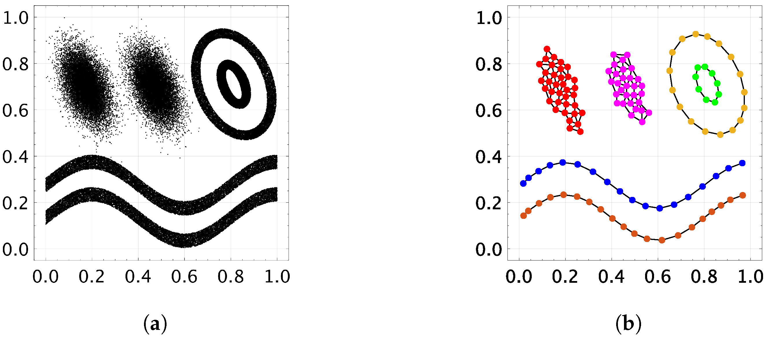
To visually understand the functionality of CAEA, Figure 4 shows a self-organization result for a synthetic dataset. The dataset consists of six distributions, and each distribution has 15,000 data points. Each data point is given to CAEA in random order and only once. The parameters of CAEA are set as $\lambda =50$, and $a_{\max }=50$. In Figure 4b, CAEA successfully generates six distributions by topological networks (i.e., nodes and edges).

3.4. Modifications of the CIM Computation

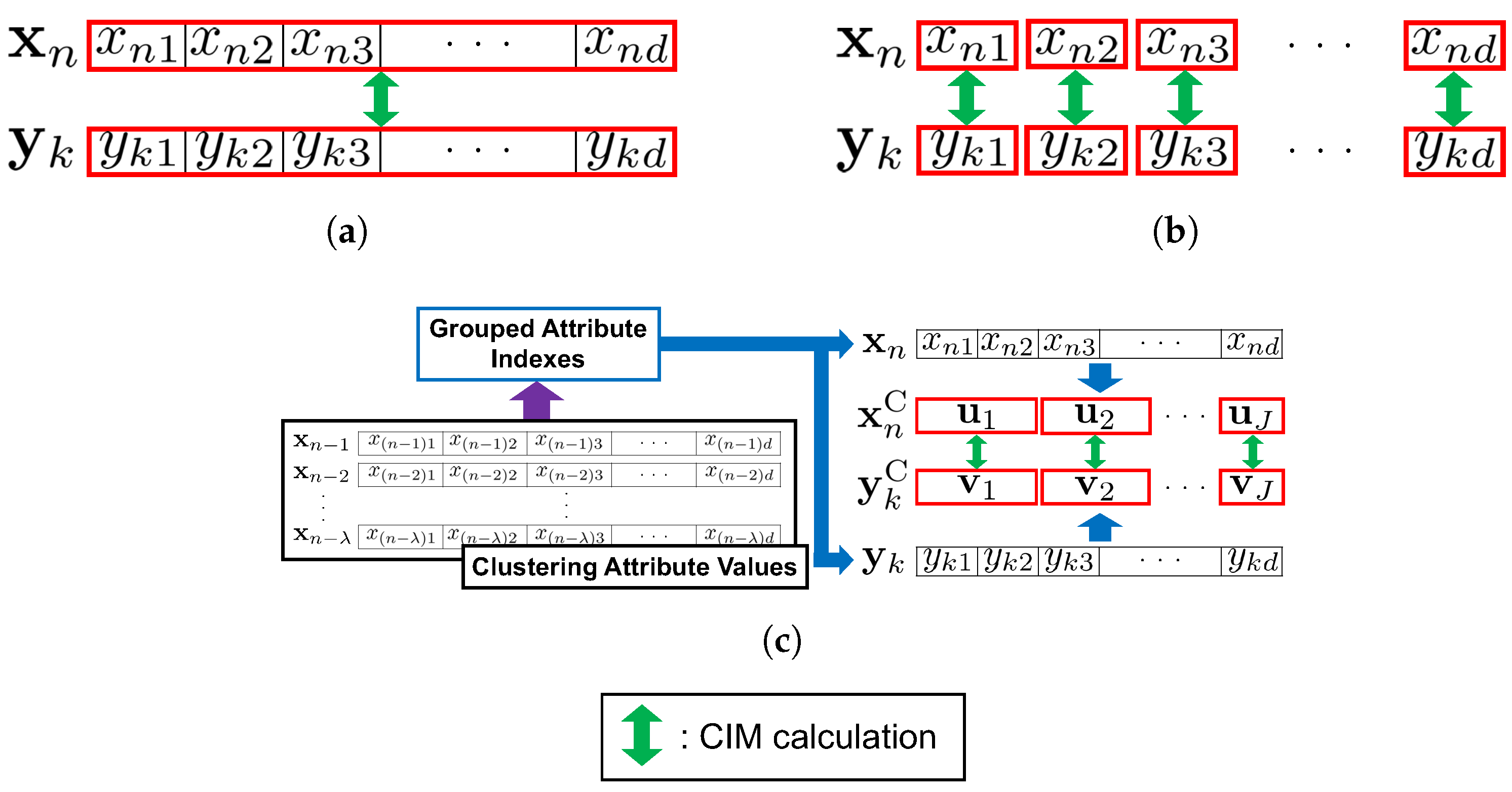
As shown in (2) and (3), the CIM in CAEAC uses a common bandwidth $\sigma$ for all attributes. Thus, a specific attribute may have a large impact on the value of the CIM if the common bandwidth $\sigma$ is not appropriate for the attribute.

In this paper, two modifications of the CIM computation [48] are integrated into CAEAC in order to mitigate the above-mentioned effects: (1) One is to compute the CIM by using each individual attribute separately, and the average CIM value is used for similarity measurement, and (2) the other is to apply a clustering algorithm to attribute values, then attributes with similar value ranges are grouped. The CIM is computed by using each attribute group, and the average CIM value is used for similarity measurement.

3.4.1. Individual-Based Approach

In this approach, the CIM is computed by using each individual attribute separately, and the average CIM value is used for similarity measurement. The similarity between a data point ${\mathbf{x}}_n$ and a node ${\mathbf{y}}_k$ is defined by the ${\mathrm{CIM}}^{\mathrm{I}}$ as follows:

$${\mathrm{CIM}}^{\mathrm{I}}\left({\mathbf{x}}_n,{\mathbf{y}}_k,{\sigma }_k\right)=\frac{1}{d}\sum _{i=1}^d{\left[{\kappa }_{{\sigma }_{k,i}}\left(0\right)-{\widehat{\mathrm{C}}}_{\mathrm{E}}^{\mathrm{I}}(x_{ni},y_{ki})\right]}^{\frac{1}{2}},$$

(22)

$${\widehat{\mathrm{C}}}_{\mathrm{E}}^{\mathrm{I}}(x_{ni},y_{ki})={\kappa }_{{\sigma }_{ki}}\left(x_{ni}-y_{ki}\right),$$

(23)

where ${\sigma }_k=\left({\sigma }_{k1},{\sigma }_{k2},\dots ,{\sigma }_{kd}\right)$ is a bandwidth of a node ${\mathbf{y}}_k$. A bandwidth for the ith attribute of ${\mathbf{y}}_k$ (i.e., ${\sigma }_{ki}$) is defined as follows:

$${\sigma }_{ki}={\left(\frac{4}{2+d}\right)}^{\frac{1}{4+d}}{\mathsf{\Gamma }}_i{\lambda }^{-\frac{1}{4+d}},$$

(24)

where ${\mathsf{\Gamma }}_i$ denotes a rescale operator, which is defined by a standard deviation of the ith attribute values among the $\lambda$ data points.

In this paper, CAEAC with the individual-based approach is called CAEAC-Individual (CAEAC-I).

3.4.2. Clustering-Based Approach

In this approach, for every $\lambda$ data points, the clustering algorithm presented in [48] is applied to the attribute values. Each attribute value of $\lambda$ data points is regarded as a one-dimensional vector and used as an input to the clustering algorithm. As a result, attributes with similar value ranges are grouped together. By using this grouping information, the similarity is calculated for each attribute group, and their average is defined as the similarity between a data point ${\mathbf{x}}_n$ and a node ${\mathbf{y}}_k$. Specifically, by using the grouping information, the data point ${\mathbf{x}}_n=$$\left(x_{n1},x_{n2},\dots ,x_{nd}\right)$ is transformed into ${\mathbf{x}}_n^{\mathrm{C}}=\left({\mathbf{u}}_{n1},{\mathbf{u}}_{n2},\dots ,{\mathbf{u}}_{nJ}\right)$$\left(J\le d\right)$ by the clustering algorithm, where ${\mathbf{u}}_j$ represents the jth attribute group. Similarly, the node ${\mathbf{y}}_k$ is transformed into ${\mathbf{y}}_k^{\mathrm{C}}=\left({\mathbf{v}}_{k1},{\mathbf{v}}_{k2},\dots ,{\mathbf{v}}_{kJ}\right)$$\left(J\le d\right)$, where ${\mathbf{v}}_j$ represents the jth attribute group. The dimensionality of each attribute group is represented as $d^{\mathrm{C}}=\{d_1,d_2,\dots ,d_J\}$, where $d_j$ is the dimensionality of the jth attribute group (i.e., the number of attributes in the jth attribute group).

Here, the similarity between the data point ${\mathbf{x}}_n^{\mathrm{C}}$ and the node ${\mathbf{y}}_k$ is defined by the ${\mathrm{CIM}}^{\mathrm{C}}$ as follows:

$${\mathrm{CIM}}^{\mathrm{C}}\left({\mathbf{x}}_n^{\mathrm{C}},{\mathbf{y}}_k^{\mathrm{C}},{\sigma }_k^{\mathrm{C}}\right)=\frac{1}{J}\sum _{j=1}^J{\left[{\kappa }_{{\sigma }_j}\left(0\right)-{\widehat{\mathrm{C}}}_{\mathrm{E}}^{\mathrm{C}}({\mathbf{u}}_j,{\mathbf{v}}_j)\right]}^{\frac{1}{2}},$$

(25)

$${\widehat{\mathrm{C}}}_{\mathrm{E}}^{\mathrm{E}}({\mathbf{u}}_j,{\mathbf{v}}_j)=\frac{1}{d_j}\sum _{i=1}^{d_j}{\kappa }_{{\sigma }_j}\left(u_i-v_i\right),$$

(26)

where ${\mathbf{y}}_k^{\mathrm{C}}=\left({\mathbf{v}}_1,{\mathbf{v}}_2,\dots ,{\mathbf{v}}_J\right)$ is a node ${\mathbf{y}}_k$, but its attributes are grouped based on the attribute grouping of ${\mathbf{x}}_n^{\mathrm{C}}$. A bandwidth ${\sigma }_j$ is defined as follows:

$${\sigma }_j=\frac{1}{d_j}\sum _{i=1}^{d_j}\left[{\left(\frac{4}{2+d_j}\right)}^{\frac{1}{4+d_j}}{\mathsf{\Gamma }}_i{\lambda }^{-\frac{1}{4+d_j}}\right],$$

(27)

where ${\mathsf{\Gamma }}_i$ denotes a rescale operator which is defined by the standard deviation of the ith attribute value in the jth attribute group among the $\lambda$ data points.

In this paper, CAEAC with the clustering-based approach is called CAEAC-Clustering (CAEAC-C).

The differences in attribute processing among the general approach, the individual-based approach (CAEAC-I), and the clustering-based approach (CAEAC-C) are shown in Figure 5. The source codes of CAEAC, CAEAC-I, and CAEAC-C are available on GitHub (https://github.com/Masuyama-lab/CAEAC, accessed on 21 September 2023).

4. Simulation Experiments

This section presents quantitative comparisons for the classification performance of ASC [8], GSOINN+ [10], CAEAC, CAEAC-I, and CAEAC-C. The source codes of ASC (https://cs.nju.edu.cn/rinc/Soinn.html, accessed on 21 September 2023) and GSOINN+ (https://osf.io/gqxya/, accessed on 21 September 2023) were provided by the authors of the related papers. ASC has a similar architecture to CAEAC (see Figure 2). GSOINN+ is the state-of-the-art SOINN-based classification algorithm capable of continual learning.

With respect to clustering algorithms, FTCA [15] is a state-of-the-art ART-based clustering algorithm while SOINN+ [20] is a state-of-the-art GNG-based clustering algorithm. The functionality of these algorithms is similar to CAEA, i.e., the algorithms adaptively and continually generate nodes and edges based on given data. Therefore, we defined the same architecture as CAEAC (see Figure 1) by using FTCA and SOINN+, called FTCA Classifier (FTCAC) and SOINN+ Classifier (SOINN + C), and used them as compared algorithms in our computational experiments. The source codes of FTCA (https://github.com/Masuyama-lab/FTCA, accessed on 21 September 2023) and SOINN+ (https://osf.io/6dqu9/, accessed on 21 September 2023) were provided by the authors of the related papers.

4.1. Datasets

We utilized five synthetic datasets and nine real-world datasets selected from the commonly used clustering benchmarks [49] and public repositories [50,51].

Table 2. Statistics of datasets for classification tasks.

Type	Dataset	Number of	Number of	Number of
		Attributes	Classes	Instances
Synthetic	Aggregation	2	7	788
	Compound	2	6	399
	Hard Distribution	2	3	1500
	Jain	2	2	373
	Pathbased	2	3	300
Real-world	ALLAML	7129	2	72
	COIL20	1024	20	1440
	Iris	4	3	150
	Isolet	617	26	7797
	OptDigits	64	10	5620
	Seeds	7	3	210
	Semeion	256	10	1593
	Sonar	60	2	208
	TOX171	5748	4	171

summarizes statistics of the datasets.

4.2. Parameter Specifications

This section describes the parameter settings of each algorithm for classification tasks in Section 4.3. ASC, FTCA, GSOINN+, CAEAC, CAEAC-I, and CAEAC-C have parameters that effect the classification performance while SOINN + C does not have any parameters.

Table 3. Parameter settings of each algorithm.

Algorithm	Parameter	Value	Grid Range	Note
ASC	$\lambda$	grid search	{20, 40, …, 400}	a node insertion cycle
	$a_{\max }$	grid search	{2, 4, …, 40}	a maximum age of edge
	k	1	—	a parameter for noise reduction
FTCAC	$\lambda$	grid search	{20, 40, …, 400}	a topology construction cycle
	V	grid search	{0.01, 0.05, 0.10, …, 0.95}	similarity threshold
GSOINN+	p	grid search	{0.01, 0.05, 0.1, 0.3, 0.5, 0.7, 0.9, 1, 2, 5, 10}	a parameter for fractional distance
	k	grid search	{1, 2, …, 10}	the number of nearest neighbors for classification
CAEAC	$\lambda$	grid search	{10, 20, …, 100}	an interval for adapting $\sigma$
	$a_{\max }$	grid search	{2, 4, …, 20}	a maximum age of edge
CAEAC-I	$\lambda$	grid search	{10, 20, …, 100}	an interval for adapting $\sigma$
	$a_{\max }$	grid search	{2, 4, …, 20}	a maximum age of edge
CAEAC-C	$\lambda$	grid search	{10, 20, …, 100}	an interval for adapting $\sigma$
	$a_{\max }$	grid search	{2, 4, …, 20}	a maximum age of edge

summarizes the parameters of each algorithm. Because SOINN + C does not have any parameters, it is not listed in Table 3. In each algorithm, two parameters are specified by a grid search. The ranges of the grid search are the same as in the original paper of each algorithm, or wider. In ASC, a parameter k for noise reduction is the same setting as in [8]. During the grid search in our experiments, the training data points in each dataset were presented to each algorithm only once without pre-processing. For each parameter specification, we repeated the evaluation 20 times. In each of the 20 runs, first, training data points with no pre-processing were randomly ordered using a different random seed. Then, the re-ordered training data points were used for all algorithms.

Table 4. Parameters specified by grid search.

Type	Dataset	ASC		FTCAC		GSOINN+		CAEAC		CAEAC-I		CAEAC-C
		$\mathbf{\lambda }$	${\mathit{a}}_{\mathbf{max}}$	$\mathbf{\lambda }$	V	p	k	$\mathbf{\lambda }$	${\mathit{a}}_{\mathbf{max}}$	$\mathbf{\lambda }$	${\mathit{a}}_{\mathbf{max}}$	$\mathbf{\lambda }$	${\mathit{a}}_{\mathbf{max}}$
Synthetic	Aggregation	140	34	360	0.90	0.50	4	90	4	100	20	50	14
	Compound	400	4	320	0.95	0.70	1	70	12	60	18	70	10
	Hard Distribution	20	10	100	0.35	0.05	7	90	6	100	18	30	8
	Jain	20	34	380	0.85	0.01	1	40	6	30	16	20	10
	Pathbased	240	6	240	0.85	0.05	2	60	14	60	6	70	2
Real-world	ALLAML	20	14	160	0.95	0.70	2	70	10	80	4	80	10
	COIL20	240	38	100	0.40	0.50	2	90	12	90	12	100	4
	Iris	280	30	400	0.70	0.05	3	90	12	90	12	10	20
	Isolet	40	8	360	0.70	10.00	2	100	6	70	12	100	20
	OptDigits	360	10	320	0.70	0.70	2	90	16	90	4	90	20
	Seeds	400	14	320	0.65	5.00	7	90	18	90	2	80	2
	Semeion	340	12	260	0.50	0.01	2	80	10	80	18	80	16
	Sonar	160	4	360	0.55	0.10	1	100	4	60	10	60	8
	TOX171	40	38	N/A		0.70	1	70	14	70	14	100	12

N/A indicates that the corresponding algorithm could not build a predictive model.

summarizes the parameter values that were specified by the grid search. N/A indicates that the corresponding algorithm could not build a predictive model. Using the parameter specifications in Table 3 and Table 4, each algorithm shows the highest accuracy for each dataset.

4.3. Classification Tasks

4.3.1. Conditions

Using the parameters in Table 3 and Table 4, we repeated the evaluation 20 times. Similar to Section 4.2, first, training data points with no pre-processing were randomly ordered using a different random seed. Then, the re-ordered training data points were used for all algorithms. The classification performance was evaluated by accuracy, NMI [52], and the Adjusted Rand Index (ARI) [53].

As a statistical analysis, the Friedman test and Nemenyi post hoc analysis [54] were utilized. The Friedman test is used to test the null hypothesis that all algorithms perform equally. If the null hypothesis is rejected, the Nemenyi post hoc analysis is conducted. The Nemenyi post hoc analysis was used for all pairwise comparisons based on the ranks of results over all the evaluation metrics for all datasets. Here, the null hypothesis was rejected at the significance level of $0.05$ both in the Friedman test and the Nemenyi post hoc analysis. All computations were carried out on Matlab 2020a with a 2.2 GHz Xeon Gold 6238R processor and 768 GB RAM.

4.3.2. Results

Table 5. Results of the classification performance.

Type	Dataset	Metric	ASC	FTCAC	SOINN + C	GSOINN+	CAEAC	CAEAC-I	CAEAC-C
Synthetic	Aggregation	Accuracy	0.999 (0.003)	0.997 (0.007)	0.997 (0.006)	0.997 (0.005)	0.998 (0.006)	0.998 (0.006)	0.999 (0.004)
		NMI	0.999 (0.006)	0.995 (0.012)	0.993 (0.012)	0.994 (0.011)	0.997 (0.011)	0.996 (0.013)	0.997 (0.008)
		ARI	0.998 (0.007)	0.994 (0.015)	0.994 (0.012)	0.994 (0.012)	0.995 (0.015)	0.997 (0.012)	0.998 (0.008)
		Training Time	0.100 (0.106)	0.013 (0.000)	2.385 (0.150)	2.019 (1.183)	0.031 (0.033)	0.252 (0.430)	0.242 (0.506)
		# of Nodes	38.8 (3.4)	151.8 (5.7)	113.0 (11.3)	58.7 (14.6)	301.0 (23.2)	310.9 (8.6)	217.4 (8.4)
		# of Clusters	—	24.5 (3.2)	31.0 (6.4)	10.1 (2.5)	240.7 (22.7)	270.9 (6.0)	92.5 (9.5)
	Compound	Accuracy	0.975 (0.026)	0.951 (0.032)	0.976 (0.024)	0.937 (0.054)	0.986 (0.021)	0.986 (0.015)	0.983 (0.020)
		NMI	0.963 (0.034)	0.927 (0.042)	0.963 (0.034)	0.922 (0.059)	0.978 (0.030)	0.974 (0.028)	0.968 (0.035)
		ARI	0.957 (0.044)	0.912 (0.054)	0.959 (0.042)	0.898 (0.093)	0.975 (0.037)	0.976 (0.026)	0.966 (0.039)
		Training Time	0.052 (0.002)	0.008 (0.002)	0.559 (0.101)	0.658 (0.136)	0.012 (0.000)	0.098 (0.155)	0.131 (0.280)
		# of Nodes	45.9 (2.9)	71.9 (2.8)	79.5 (10.8)	42.1 (11.0)	188.5 (11.5)	175.4 (3.1)	198.2 (4.7)
		# of Clusters	—	13.7 (2.3)	32.1 (9.6)	11.6 (6.3)	154.6 (9.2)	156.0 (5.4)	130.7 (4.8)
	Hard Distribution	Accuracy	0.991 (0.007)	0.996 (0.005)	0.993 (0.009)	0.991 (0.007)	0.992 (0.006)	0.992 (0.006)	0.992 (0.005)
		NMI	0.962 (0.028)	0.982 (0.023)	0.970 (0.035)	0.962 (0.027)	0.967 (0.026)	0.966 (0.025)	0.967 (0.021)
		ARI	0.974 (0.019)	0.988 (0.015)	0.978 (0.026)	0.973 (0.020)	0.977 (0.018)	0.977 (0.017)	0.977 (0.016)
		Training Time	0.203 (0.113)	0.023 (0.020)	3.134 (0.419)	3.036 (0.355)	0.066 (0.046)	0.905 (1.668)	0.556 (0.663)
		# of Nodes	10.3 (1.1)	47.3 (3.7)	103.4 (24.2)	63.4 (18.0)	197.8 (21.0)	219.9 (8.0)	80.1 (5.3)
		# of Clusters	—	3.8 (1.0)	13.8 (5.8)	6.4 (2.5)	75.8 (21.1)	97.9 (11.5)	12.7 (4.2)
	Jain	Accuracy	0.883 (0.127)	0.988 (0.016)	1.000 (0.000)	1.000 (0.000)	1.000 (0.000)	1.000 (0.000)	1.000 (0.000)
		NMI	0.612 (0.283)	0.921 (0.106)	1.000 (0.000)	1.000 (0.000)	1.000 (0.000)	1.000 (0.000)	1.000 (0.000)
		ARI	0.627 (0.326)	0.948 (0.071)	1.000 (0.000)	1.000 (0.000)	1.000 (0.000)	1.000 (0.000)	1.000 (0.000)
		Training Time	0.038 (0.001)	0.007 (0.001)	0.773 (0.210)	0.624 (0.105)	0.010 (0.001)	0.182 (0.355)	0.484 (0.800)
		# of Nodes	6.0 (0.8)	76.2 (4.1)	49.4 (9.6)	39.5 (13.6)	46.1 (4.0)	42.0 (6.5)	31.1 (3.1)
		# of Clusters	—	14.5 (2.6)	14.7 (6.1)	10.4 (5.4)	20.4 (3.0)	20.9 (6.9)	8.5 (2.8)
	Pathbased	Accuracy	0.993 (0.014)	0.937 (0.043)	0.970 (0.036)	0.967 (0.046)	0.992 (0.015)	0.990 (0.022)	0.987 (0.020)
		NMI	0.980 (0.042)	0.830 (0.108)	0.912 (0.104)	0.913 (0.097)	0.975 (0.045)	0.969 (0.066)	0.958 (0.062)
		ARI	0.980 (0.042)	0.816 (0.123)	0.909 (0.108)	0.904 (0.120)	0.976 (0.043)	0.970 (0.064)	0.958 (0.062)
		Training Time	0.033 (0.002)	0.006 (0.000)	0.420 (0.081)	0.463 (0.096)	0.010 (0.000)	0.192 (0.263)	0.095 (0.202)
		# of Nodes	30.3 (2.8)	64.7 (5.9)	51.9 (9.8)	30.8 (6.6)	104.9 (5.9)	102.4 (3.1)	114.9 (3.3)
		# of Clusters	—	17.6 (3.2)	18.6 (7.9)	7.4 (3.9)	76.9 (4.3)	80.6 (3.9)	63.8 (4.0)
Real-world	ALLAML	Accuracy	0.915 (0.134)	0.911 (0.112)	0.770 (0.180)	0.799 (0.146)	0.890 (0.096)	0.887 (0.110)	0.888 (0.107)
		NMI	0.721 (0.372)	0.720 (0.339)	0.407 (0.388)	0.304 (0.378)	0.586 (0.356)	0.591 (0.347)	0.595 (0.374)
		ARI	0.675 (0.430)	0.680 (0.385)	0.357 (0.412)	0.268 (0.370)	0.540 (0.387)	0.537 (0.384)	0.577 (0.386)
		Training Time	0.144 (0.019)	0.173 (0.007)	0.098 (0.012)	0.149 (0.040)	0.684 (0.026)	4.075 (7.105)	2.247 (2.489)
		# of Nodes	4.3 (0.7)	4.0 (0.0)	20.6 (4.0)	11.7 (3.3)	60.5 (1.4)	63.5 (0.9)	62.5 (1.4)
		# of Clusters	—	2.0 (0.0)	17.2 (4.1)	9.6 (3.2)	57.5 (2.5)	62.9 (1.4)	60.2 (2.7)
	COIL20	Accuracy	0.992 (0.007)	0.952 (0.024)	0.951 (0.018)	0.850 (0.050)	1.000 (0.000)	1.000 (0.000)	0.996 (0.007)
		NMI	0.993 (0.007)	0.960 (0.018)	0.962 (0.014)	0.894 (0.032)	1.000 (0.000)	1.000 (0.000)	0.996 (0.007)
		ARI	0.983 (0.017)	0.912 (0.044)	0.912 (0.037)	0.739 (0.089)	1.000 (0.000)	1.000 (0.000)	0.991 (0.016)
		Training Time	3.106 (0.087)	0.545 (0.015)	1.603 (0.186)	2.938 (0.286)	1.409 (0.048)	11.990 (20.749)	5.679 (8.093)
		# of Nodes	326.5 (14.6)	103.7 (5.7)	318.7 (14.9)	98.2 (18.4)	1069.4 (14.1)	1055.6 (10.7)	1001.0 (0.9)
		# of Clusters	—	24.4 (2.0)	155.0 (15.5)	34.0 (7.8)	965.1 (19.9)	940.1 (18.2)	974.1 (1.5)
	Iris	Accuracy	0.973 (0.040)	0.977 (0.039)	0.937 (0.063)	0.967 (0.055)	0.963 (0.046)	0.963 (0.046)	0.977 (0.039)
		NMI	0.934 (0.097)	0.944 (0.090)	0.854 (0.145)	0.921 (0.129)	0.917 (0.097)	0.917 (0.097)	0.942 (0.096)
		ARI	0.922 (0.115)	0.923 (0.128)	0.823 (0.183)	0.899 (0.170)	0.888 (0.138)	0.888 (0.138)	0.932 (0.115)
		Training Time	0.022 (0.001)	0.004 (0.000)	0.128 (0.030)	0.214 (0.050)	0.006 (0.000)	0.052 (0.148)	0.182 (0.267)
		# of Nodes	12.1 (1.5)	25.7 (2.6)	37.1 (6.6)	22.1 (5.2)	134.0 (1.1)	134.1 (0.9)	21.5 (1.9)
		# of Clusters	—	5.5 (1.4)	19.9 (5.8)	8.7 (4.1)	133.7 (1.7)	133.7 (1.7)	7.2 (1.7)
	Isolet	Accuracy	0.904 (0.010)	0.909 (0.012)	0.823 (0.015)	0.739 (0.029)	0.852 (0.014)	0.842 (0.013)	0.881 (0.012)
		NMI	0.898 (0.010)	0.900 (0.010)	0.832 (0.012)	0.778 (0.022)	0.858 (0.010)	0.848 (0.010)	0.880 (0.009)
		ARI	0.821 (0.021)	0.829 (0.023)	0.695 (0.025)	0.593 (0.041)	0.740 (0.021)	0.722 (0.021)	0.784 (0.024)
		Training Time	13.601 (0.430)	2.191 (0.080)	4.358 (0.333)	11.282 (4.310)	7.468 (0.068)	19.951 (23.957)	29.610 (17.282)
		# of Nodes	401.6 (22.4)	164.9 (6.6)	718.8 (40.8)	189.4 (52.1)	2003.8 (18.7)	1556.9 (47.6)	2449.2 (22.8)
		# of Clusters	—	34.8 (3.2)	462.5 (27.3)	94.6 (28.4)	1574.6 (17.3)	1198.1 (47.5)	1444.7 (32.8)
	OptDigits	Accuracy	0.988 (0.005)	0.982 (0.005)	0.969 (0.009)	0.959 (0.008)	0.974 (0.007)	0.972 (0.005)	0.975 (0.009)
		NMI	0.975 (0.009)	0.962 (0.011)	0.938 (0.015)	0.921 (0.013)	0.946 (0.013)	0.943 (0.010)	0.949 (0.016)
		ARI	0.974 (0.010)	0.960 (0.012)	0.932 (0.019)	0.913 (0.017)	0.943 (0.015)	0.938 (0.012)	0.945 (0.019)
		Training Time	1.286 (0.028)	0.643 (0.011)	4.932 (0.289)	6.160 (0.695)	0.650 (0.011)	4.042 (4.549)	6.645 (10.283)
		# of Nodes	638.0 (21.2)	1241.2 (13.7)	487.3 (31.8)	222.2 (34.0)	819.3 (12.9)	719.9 (22.6)	769.3 (16.1)
		# of Clusters	—	36.8 (5.8)	176.5 (16.3)	56.9 (10.9)	453.2 (15.4)	463.2 (16.9)	352.3 (16.5)
	Seeds	Accuracy	0.895 (0.061)	0.912 (0.054)	0.900 (0.055)	0.924 (0.064)	0.921 (0.062)	0.921 (0.068)	0.926 (0.063)
		NMI	0.760 (0.126)	0.781 (0.120)	0.758 (0.139)	0.811 (0.143)	0.806 (0.142)	0.815 (0.143)	0.815 (0.141)
		ARI	0.715 (0.160)	0.750 (0.141)	0.750 (0.143)	0.788 (0.173)	0.782 (0.164)	0.794 (0.155)	0.790 (0.167)
		Training Time	0.025 (0.001)	0.005 (0.000)	0.213 (0.041)	0.328 (0.066)	0.009 (0.000)	0.132 (0.281)	0.050 (0.136)
		# of Nodes	16.5 (2.1)	34.0 (4.2)	40.8 (6.9)	25.2 (7.3)	164.5 (3.9)	159.7 (4.1)	120.9 (0.9)
		# of Clusters	—	5.9 (1.7)	18.8 (5.6)	6.7 (4.1)	156.4 (6.0)	148.8 (7.0)	75.8 (2.8)
	Semeion	Accuracy	0.924 (0.023)	0.916 (0.018)	0.819 (0.032)	0.720 (0.038)	0.889 (0.033)	0.886 (0.027)	0.884 (0.029)
		NMI	0.887 (0.031)	0.873 (0.027)	0.753 (0.034)	0.660 (0.039)	0.838 (0.041)	0.834 (0.037)	0.831 (0.036)
		ARI	0.841 (0.045)	0.826 (0.035)	0.650 (0.050)	0.512 (0.051)	0.772 (0.062)	0.768 (0.057)	0.761 (0.056)
		Training Time	0.679 (0.022)	0.267 (0.010)	0.824 (0.066)	0.854 (0.142)	0.394 (0.009)	3.514 (4.117)	0.896 (0.894)
		# of Nodes	234.8 (11.0)	195.9 (7.4)	231.2 (20.8)	86.5 (19.0)	596.7 (13.4)	586.2 (13.9)	579.2 (9.1)
		# of Clusters	—	21.8 (2.7)	144.9 (15.9)	45.8 (12.0)	432.1 (18.2)	402.5 (16.4)	534.5 (12.6)
	Sonar	Accuracy	0.803 (0.080)	0.739 (0.126)	0.702 (0.108)	0.753 (0.074)	0.827 (0.090)	0.822 (0.117)	0.836 (0.077)
		NMI	0.329 (0.187)	0.246 (0.207)	0.179 (0.160)	0.235 (0.154)	0.385 (0.217)	0.438 (0.253)	0.421 (0.223)
		ARI	0.358 (0.208)	0.257 (0.229)	0.172 (0.183)	0.240 (0.161)	0.425 (0.235)	0.443 (0.270)	0.448 (0.226)
		Training Time	0.030 (0.001)	0.007 (0.000)	0.184 (0.034)	0.189 (0.069)	0.021 (0.001)	0.120 (0.223)	0.148 (0.307)
		# of Nodes	34.4 (4.2)	7.1 (0.9)	36.0 (8.8)	27.9 (10.3)	116.8 (27.3)	70.5 (2.8)	84.3 (5.0)
		# of Clusters	—	2.1 (0.3)	19.4 (7.0)	13.2 (6.1)	99.1 (26.5)	58.5 (4.2)	40.5 (7.3)
	TOX171	Accuracy	0.760 (0.104)	N/A	0.600 (0.138)	0.596 (0.101)	0.857 (0.077)	0.860 (0.074)	0.851 (0.082)
		NMI	0.627 (0.143)		0.481 (0.144)	0.465 (0.100)	0.769 (0.111)	0.769 (0.111)	0.761 (0.115)
		ARI	0.450 (0.206)		0.252 (0.179)	0.237 (0.141)	0.668 (0.168)	0.671 (0.167)	0.649 (0.183)
		Training Time	0.614 (0.046)		0.244 (0.030)	0.604 (0.180)	1.437 (0.111)	3.249 (1.746)	1.561 (0.330)
		# of Nodes	40.0 (5.1)		44.3 (4.6)	27.0 (7.4)	145.4 (1.1)	145.0 (1.1)	153.9 (0.3)
		# of Clusters	—		29.1 (3.8)	14.3 (5.0)	143.3 (1.9)	141.5 (2.3)	153.9 (0.3)

The standard deviation is indicated in parentheses. Training time is in [second]. The brighter the cell color, the better the performance. N/A indicates that the corresponding algorithm could not build a predictive model.

shows the results of the classification performance. The best value in each metric is indicated in bold for each dataset. The standard deviation is indicated in parentheses. N/A indicates that the corresponding algorithm could not build a predictive model. Training time is in [second]. The brighter the cell color, the better the performance. In ASC, k-means is applied to adjust the position of the generated nodes in order to achieve a good approximation of the distribution of data points. In addition, some generated nodes and edges are deleted during the learning process. Therefore, the number of clusters is not shown for ASC in Table 5.

As an overall trend, ASC, CAEAC, CAEAC-I, and CAEAC-C show better classification performance than SOINN + C, and GSOINN+. FTCAC shows the best classification performance on several datasets, whereas FTCAC cannot build a predictive model for TOX171. Regarding training time, ASC, FTCAC, and CAEAC are shorter than SOINN + C, GSOINN+, CAEAC-I, and CAEAC-C. With respect to generated nodes and clusters, CAEAC and its variants tend to generate a larger number of nodes and clusters than those of compared algorithms.

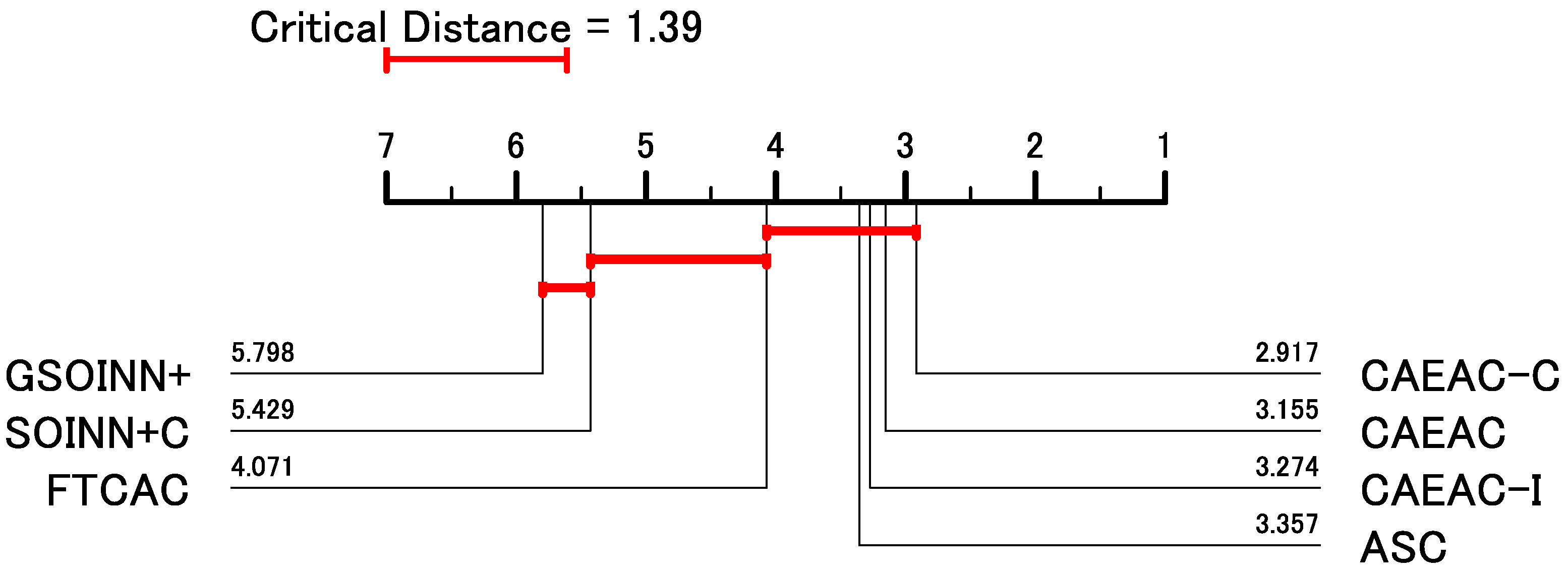
Here, the null hypothesis was rejected on the Friedman test over all the evaluation metrics and datasets. Thus, we applied the Nemenyi post hoc analysis. Figure 6 shows a critical difference diagram based on the classification performance including all the evaluation metrics and datasets. Better performance is shown by lower average ranks, i.e., on the right side of a critical distance diagram. In theory, different algorithms within a critical distance (i.e., a red line) do not have a statistically significant difference [54]. In Figure 6, CAEAC-C shows the lowest rank value, but there is no statistically significant difference from CAEAC, CAEAC-I, ASC, and FTCAC.

Among the compared algorithms, FTCAC cannot build a predictive model for TOX171 as shown in Table 5. This is a critical problem of FTCAC. SOINN + C and GSOINN+ show inferior classification performance to ASC, CAEAC, CAEAC-I, and CAEAC-C as shown in Figure 6 (and Table 5). Although ASC shows comparable classification performance to CAEAC, CAEAC-I, and CAEAC-C, ASC deletes some generated nodes and edges during its learning process. Therefore, it may be difficult for ASC to maintain continual learning capability when learning additional data points after the deletion process. This can be regarded as the functional limitation of ASC.

The effect of the different attribute processing of CAEAC and its variants shown in Figure 5 on the classification performance may be considered based on the difference in the number of clusters. In CAEAC, the difference in the range of attribute values may greatly affect the similarity measurement between a node and a given data point by CIM. Since CAEAC-I calculates similarity on each attribute, the difference in the range of each attribute value has no effect. Therefore, CAEAC-I can compute the similarity between a node and a given data point more accurately than CAEAC. On the other hand, the similarity tends to be smaller, i.e., CAEAC-I tends to generate many clusters. In CAEAC-C, the similarity measurement can be viewed as an intermediate approach between CAEAC and CAEAC-I, allowing for the suppression of excessive cluster generation while maintaining accurate similarity measures. This can be considered the reason why CAEAC-C shows superior classification performance on average to CAEAC and CAEAC-I (see Table 5).

The above observations suggest that CAEAC, CAEAC-I, and CAEAC-C have several advantages over teh compared algorithms not only in classification performance but also from a functional perspective. The characteristics of CAEAC and its variants are summarized as follows:

• CAEAC

This algorithm shows stable and good classification performance and maintains fast computation.

• CAEAC-I

The classification performance and computation time of this algorithm are both inferior to CAEAC and CAEAC-C. However, in Table 5, it has the highest number of the best evaluation metric values among CAEAC and its variants. Therefore, this algorithm is worth trying when high classification performance is desired.

• CAEAC-C

Among CAEAC and its variants, CAEAC-I showed the best classification performance on many datasets, but the worst on a couple of datasets. In contrast, according to the critical difference diagram in Figure 2, CAEAC-C shows the lowest rank, i.e., the best algorithm, based on the ranks of results over all the evaluation metrics for all datasets. This observation indicates that CAEAC-C can be the first-choice algorithm if the property of a dataset is not known.

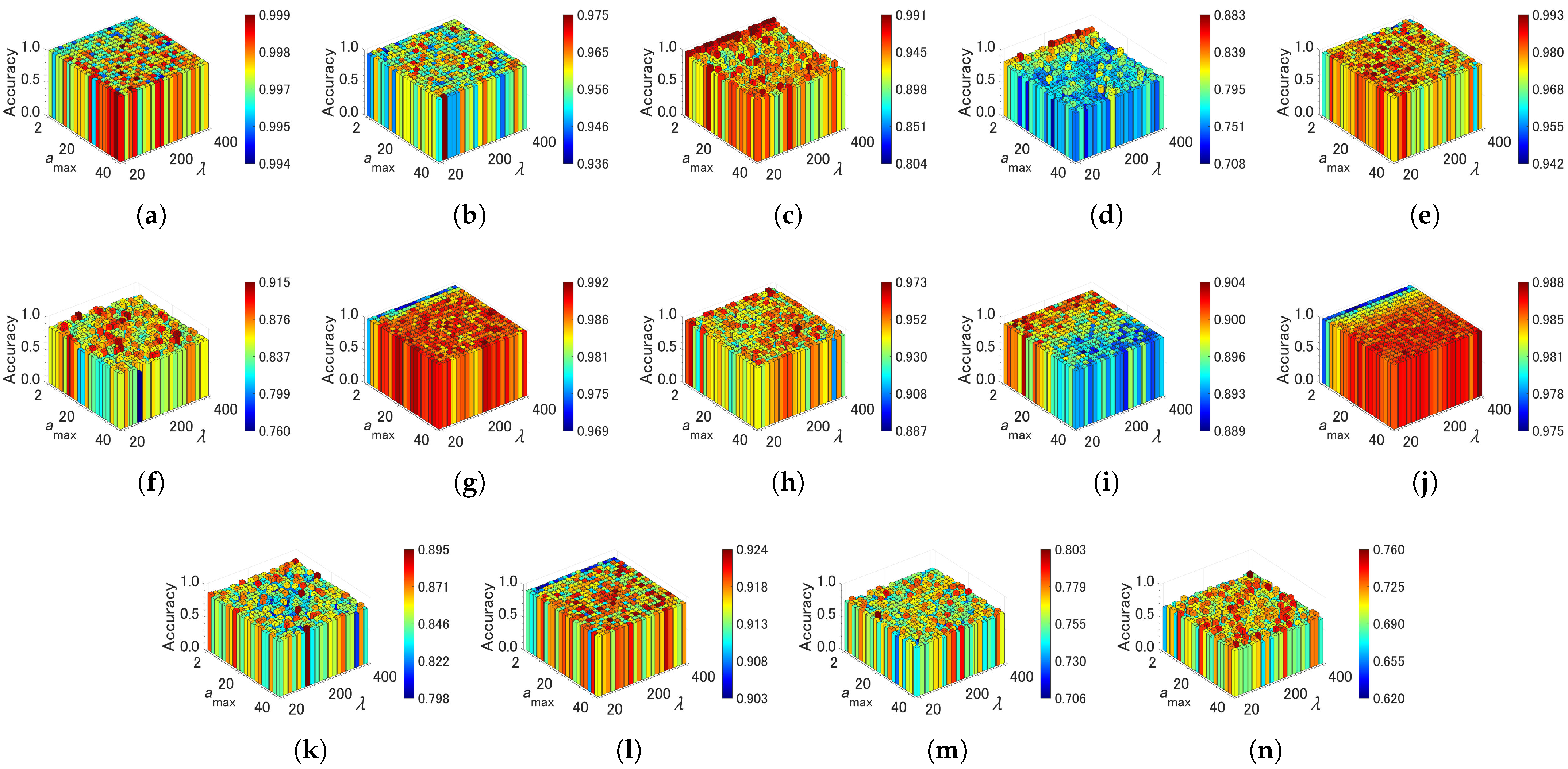
4.4. Sensitivity of Parameters

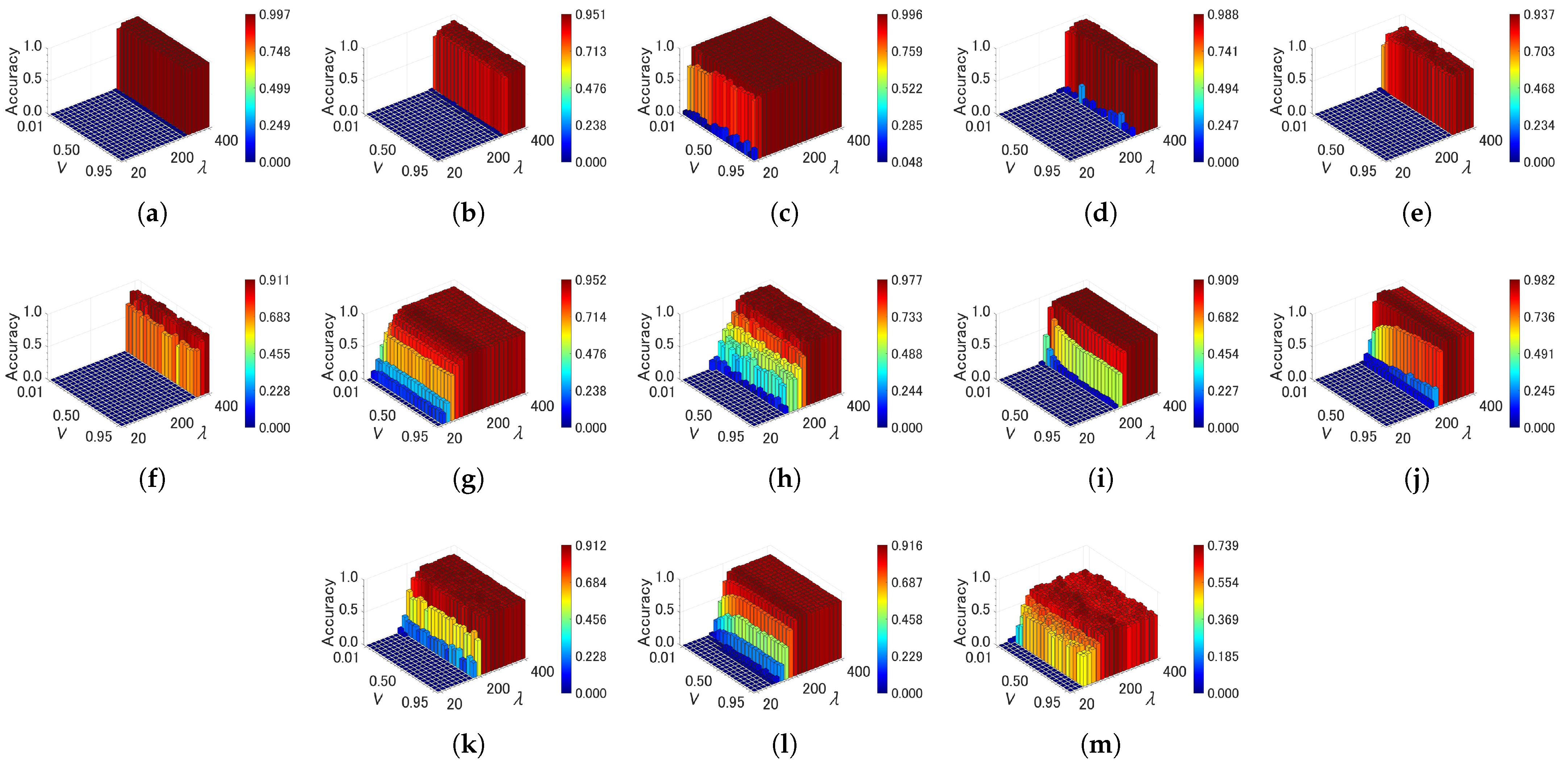
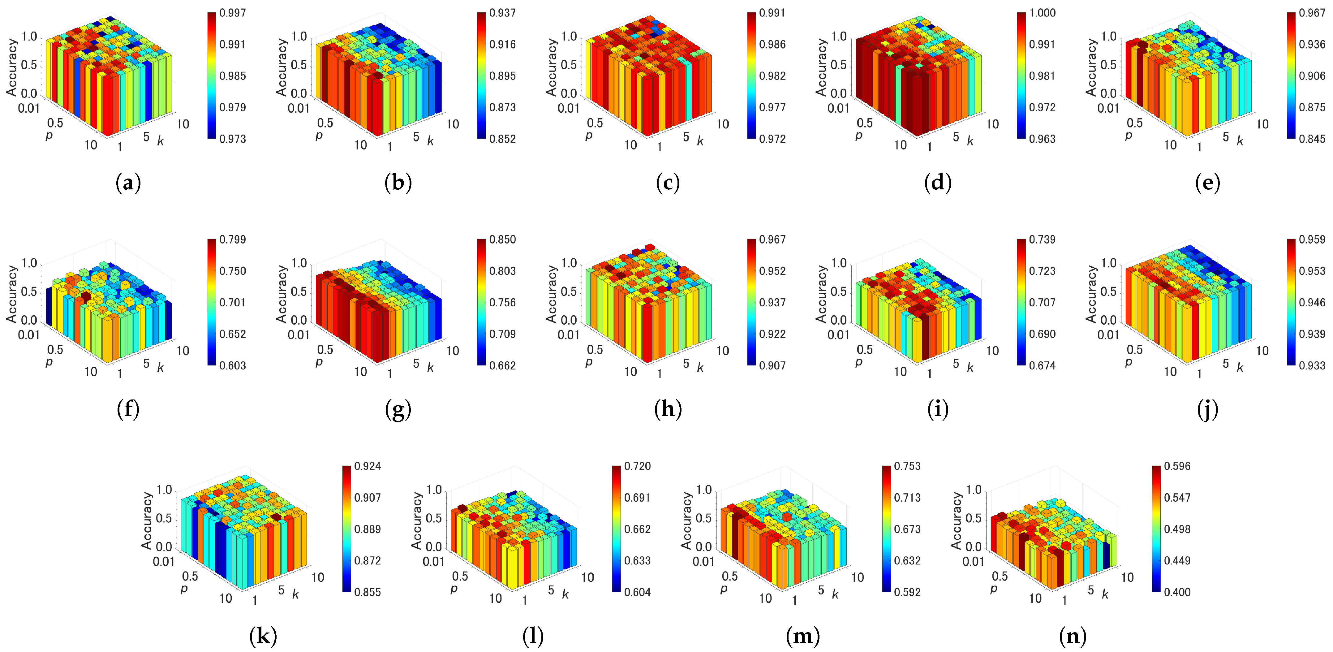
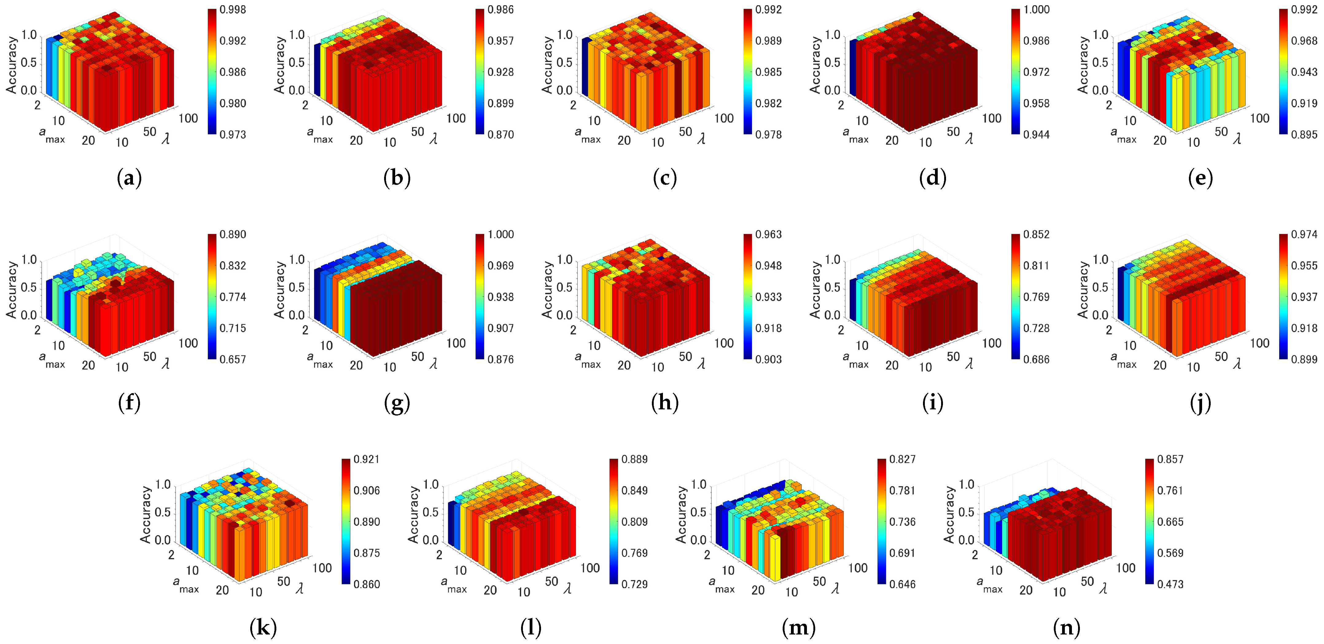
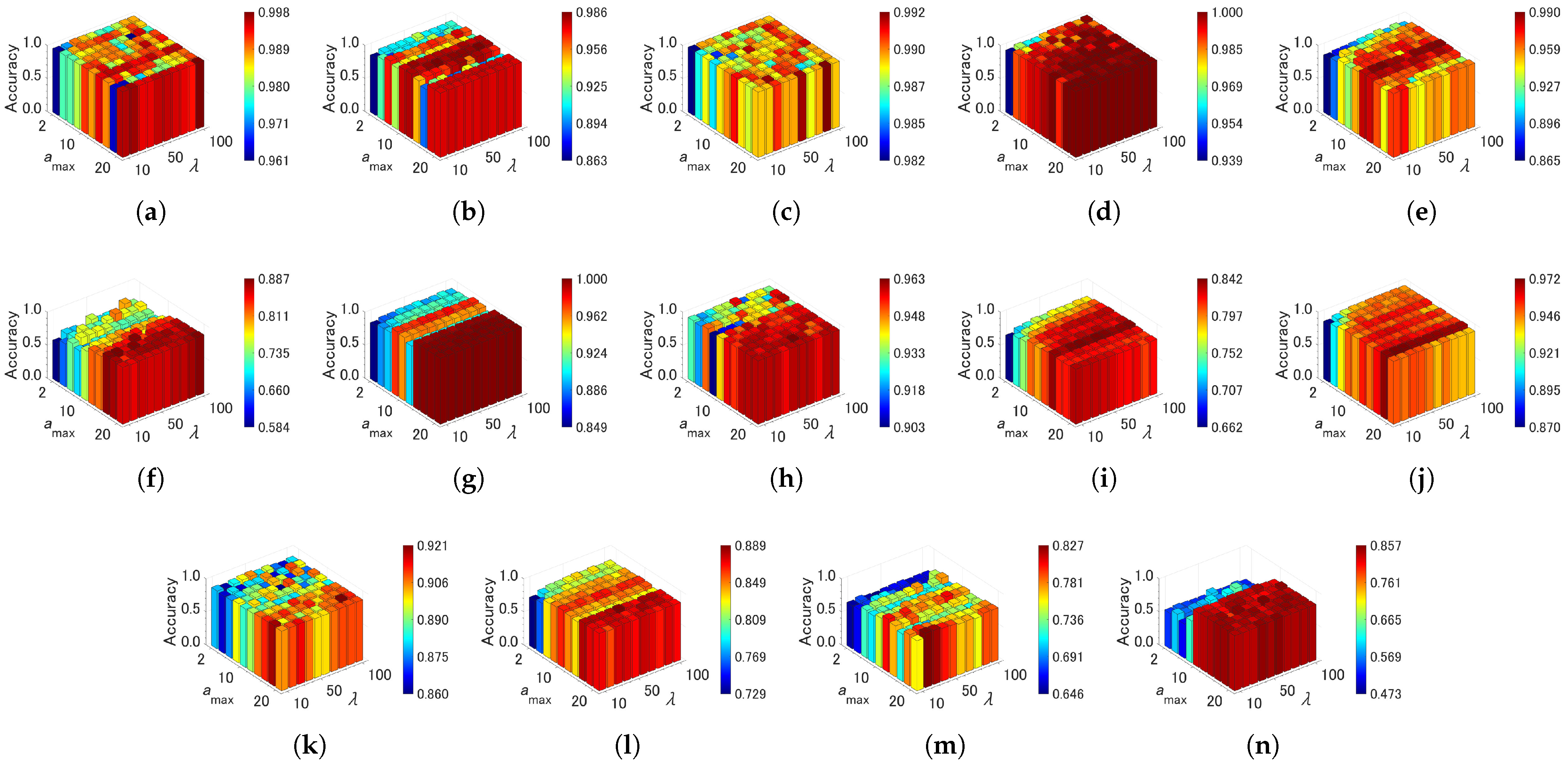
In this section, we analyze the sensitivity of parameter specifications in each algorithm from the relationships between parameter values and classification accuracy. The parameters of each algorithm are summarized in Table 3. Figure 7, Figure 8 and Figure 9 show the effects of the parameter settings on accuracy for ASC, FTCAC, and GSOINN+, respectively. In the case of ASC, accuracy varies depending on the combination of parameters for several datasets (Hard Distribution, Jain, ALLAML, Seeds, Sonar, and TOX171). This indicates that high accuracy cannot be maintained without a careful specification of parameters. With respect to FCTAC, high accuracy can be achieved for most datasets by choosing a large $\lambda$ value (e.g., $\lambda$ > 350); therefore, the parameter sensitivity of FTCAC is low for a certain range of parameters. One problem of FTCAC is that the algorithm cannot build a predictive model for TOX171 with any parameter setting. GSOINN+ shows a similar trend to ASC, i.e., a careful specification of parameters is required to achieve high accuracy on some datasets.

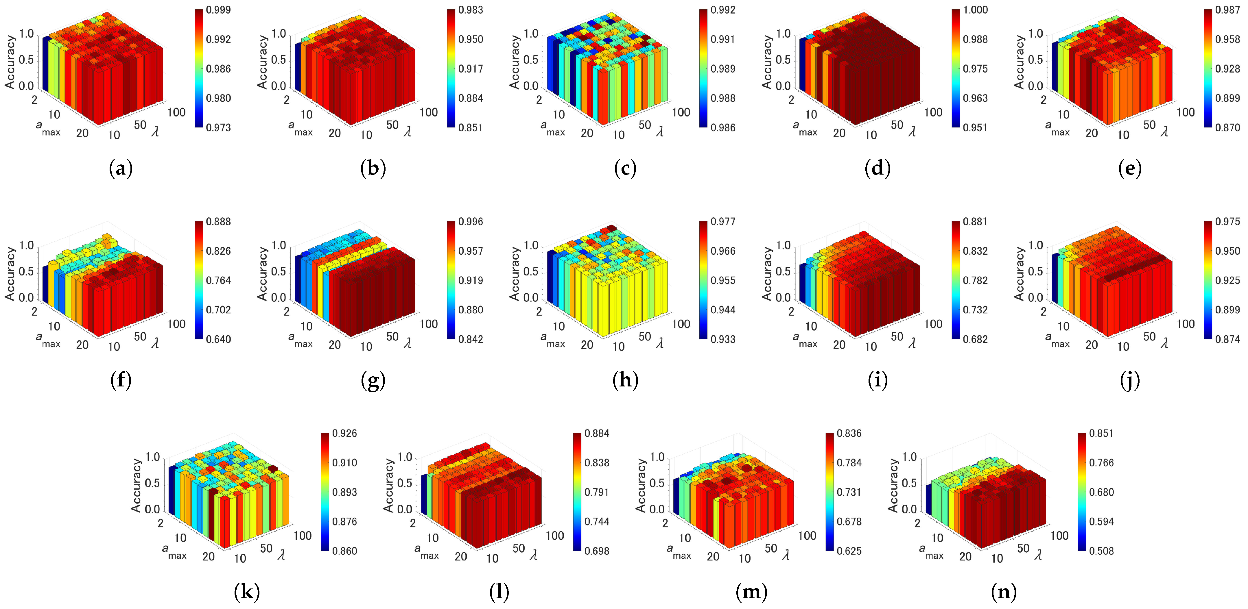
Figure 10, Figure 11 and Figure 12 show effects of the parameter settings on accuracy for CAEAC, CAEAC-I, and CAEAC-C, respectively. CAEAC and its variants have two parameters: $\lambda$ is the predefined interval for computing $\sigma$ and deleting an isolated node, and $a_{\max }$ is the predefined threshold of the age of edges. Comparing ASC and GSOINN+ with CAEAC, CAEAC shows less variance in accuracy regardless of parameter settings. CAEAC-I and CAEAC-C also show the same trend as CAEAC. This advantage is also shown in the parameter values determined by the grid search summarized in Table 4. The parameters of ASC, FTCAC, and GSOINN+ vary widely from dataset to dataset. On the other hand, the parameters of CAEAC, CAEAC-I, and CAEAC-C show less variance across datasets than in the case of the comparison algorithms.

From the above observations, the sensitivity of the parameters of FTCAC, CAEAC, CAEAC-I, and CAEAC-C are lower than ASC and GSOINN+. Moreover, it can be considered that FTCAE, CAEAC, CAEAC-I, and CAEAC-C can utilize the common parameter setting in a wide variety of datasets without the difficulty of parameter specification.

5. Conclusions

Continual learning is one of the most challenging problems in the machine learning domain. In this paper, to tackle the class incremental learning scenario in continual learning, we proposed a supervised classification algorithm capable of continual learning using an ART-based growing self-organizing clustering algorithm, called CAEAC. In addition, we also proposed the variants of CAEAC, called CAEAC-I and CAEAC-C, by modifying the CIM computation.

Experimental results of classification performance showed that CAEAC and its variants have superior classification performance to state-of-the-art clustering-based classifiers. In addition, the simple modifications of the CIM computation successfully improved the classification performance of CAEAC-I and CAEAC-C. The analysis of the parameter sensitivity in CAEAC and its variants showed that common parameter settings can be used for various data sets without difficulty in specifying parameters. The above results suggest that CAEAC and its variants have several advantages over the compared algorithms in terms of classification performance and functionality for continual learning.

The proposed algorithms accumulate data and compose classifiers using an ART-based clustering algorithm capable of continual learning. Therefore, the proposed algorithms are particularly effective when applied to systems and applications that continually generate a large amount of data.

In regard to continual learning, the concepts of learned information sometimes change over time. This is known as concept drift [55]. However, since CAEAC and its variants focus only on the class incremental learning scenario in continual learning, they may not adequately address concept drift. Thus, as a future research topic, we will develop a function for handling concept drift in CAEAC and its variants in order to improve the functionality of the algorithms.

References

- McCloskey, M.; Cohen, N.J. Catastrophic interference in connectionist networks: The sequential learning problem. Psychol. Learn. Motiv. 1989, 24, 109–165. [Google Scholar]
- Parisi, G.I.; Kemker, R.; Part, J.L.; Kanan, C.; Wermter, S. Continual lifelong learning with neural networks: A review. Neural Netw. 2019, 113, 57–71. [Google Scholar] [CrossRef] [PubMed]
- Van de Ven, G.M.; Tolias, A.S. Three scenarios for continual learning. arXiv 2019, arXiv:1904.07734. [Google Scholar]
- Wiewel, F.; Yang, B. Localizing catastrophic forgetting in neural networks. arXiv 2019, arXiv:1906.02568. [Google Scholar]
- Kirkpatrick, J.; Pascanu, R.; Rabinowitz, N.; Veness, J.; Desjardins, G.; Rusu, A.A.; Milan, K.; Quan, J.; Ramalho, T.; Grabska-Barwinska, A.; et al. Overcoming catastrophic forgetting in neural networks. Proc. Natl. Acad. Sci. USA 2017, 114, 3521–3526. [Google Scholar] [CrossRef]
- Furao, S.; Hasegawa, O. An incremental network for on-line unsupervised classification and topology learning. Neural Netw. 2006, 19, 90–106. [Google Scholar] [CrossRef] [PubMed]
- Fritzke, B. A growing neural gas network learns topologies. Adv. Neural Inf. Process. Syst. 1995, 7, 625–632. [Google Scholar]
- Shen, F.; Hasegawa, O. A fast nearest neighbor classifier based on self-organizing incremental neural network. Neural Netw. 2008, 21, 1537–1547. [Google Scholar] [CrossRef]
- Parisi, G.I.; Tani, J.; Weber, C.; Wermter, S. Lifelong learning of human actions with deep neural network self-organization. Neural Netw. 2017, 96, 137–149. [Google Scholar] [CrossRef]
- Wiwatcharakoses, C.; Berrar, D. A self-organizing incremental neural network for continual supervised learning. Expert Syst. Appl. 2021, 185, 115662. [Google Scholar] [CrossRef]
- Grossberg, S. Competitive learning: From interactive activation to adaptive resonance. Cogn. Sci. 1987, 11, 23–63. [Google Scholar] [CrossRef]
- Liu, W.; Pokharel, P.P.; Príncipe, J.C. Correntropy: Properties and applications in non-Gaussian signal processing. IEEE Trans. Signal Process. 2007, 55, 5286–5298. [Google Scholar] [CrossRef]
- Chalasani, R.; Príncipe, J.C. Self-organizing maps with information theoretic learning. Neurocomputing 2015, 147, 3–14. [Google Scholar] [CrossRef]
- Masuyama, N.; Loo, C.K.; Ishibuchi, H.; Kubota, N.; Nojima, Y.; Liu, Y. Topological Clustering via Adaptive Resonance Theory With Information Theoretic Learning. IEEE Access 2019, 7, 76920–76936. [Google Scholar] [CrossRef]
- Masuyama, N.; Amako, N.; Nojima, Y.; Liu, Y.; Loo, C.K.; Ishibuchi, H. Fast Topological Adaptive Resonance Theory Based on Correntropy Induced Metric. In Proceedings of the IEEE Symposium Series on Computational Intelligence, Xiamen, China, 6–9 December 2019; pp. 2215–2221. [Google Scholar]
- Masuyama, N.; Amako, N.; Yamada, Y.; Nojima, Y.; Ishibuchi, H. Adaptive resonance theory-based topological clustering with a divisive hierarchical structure capable of continual learning. IEEE Access 2022, 10, 68042–68056. [Google Scholar] [CrossRef]
- McLachlan, G.J.; Lee, S.X.; Rathnayake, S.I. Finite mixture models. Annu. Rev. Stat. Its Appl. 2019, 6, 355–378. [Google Scholar] [CrossRef]
- Lloyd, S. Least squares quantization in PCM. IEEE Trans. Inf. Theory 1982, 28, 129–137. [Google Scholar] [CrossRef]
- Carpenter, G.A.; Grossberg, S. The ART of adaptive pattern recognition by a self-organizing neural network. Computer 1988, 21, 77–88. [Google Scholar] [CrossRef]
- Wiwatcharakoses, C.; Berrar, D. SOINN+, a self-organizing incremental neural network for unsupervised learning from noisy data streams. Expert Syst. Appl. 2020, 143, 113069. [Google Scholar] [CrossRef]
- Marsland, S.; Shapiro, J.; Nehmzow, U. A self-organising network that grows when required. Neural Netw. 2002, 15, 1041–1058. [Google Scholar] [CrossRef]
- Tan, S.C.; Watada, J.; Ibrahim, Z.; Khalid, M. Evolutionary fuzzy ARTMAP neural networks for classification of semiconductor defects. IEEE Trans. Neural Netw. Learn. Syst. 2014, 26, 933–950. [Google Scholar] [PubMed]
- Matias, A.L.; Neto, A.R.R. OnARTMAP: A fuzzy ARTMAP-based architecture. Neural Netw. 2018, 98, 236–250. [Google Scholar] [CrossRef] [PubMed]
- Matias, A.L.; Neto, A.R.R.; Mattos, C.L.C.; Gomes, J.P.P. A novel fuzzy ARTMAP with area of influence. Neurocomputing 2021, 432, 80–90. [Google Scholar] [CrossRef]
- Carpenter, G.A.; Grossberg, S.; Rosen, D.B. Fuzzy ART: Fast stable learning and categorization of analog patterns by an adaptive resonance system. Neural Netw. 1991, 4, 759–771. [Google Scholar] [CrossRef]
- Vigdor, B.; Lerner, B. The Bayesian ARTMAP. IEEE Trans. Neural Netw. 2007, 18, 1628–1644. [Google Scholar] [CrossRef]
- Wang, L.; Zhu, H.; Meng, J.; He, W. Incremental Local Distribution-Based Clustering Using Bayesian Adaptive Resonance Theory. IEEE Trans. Neural Netw. Learn. Syst. 2019, 30, 3496–3504. [Google Scholar] [CrossRef]
- da Silva, L.E.B.; Elnabarawy, I.; Wunsch, D.C., II. Distributed dual vigilance fuzzy adaptive resonance theory learns online, retrieves arbitrarily-shaped clusters, and mitigates order dependence. Neural Netw. 2020, 121, 208–228. [Google Scholar] [CrossRef]
- Masuyama, N.; Loo, C.K.; Dawood, F. Kernel Bayesian ART and ARTMAP. Neural Netw. 2018, 98, 76–86. [Google Scholar] [CrossRef]
- Masuyama, N.; Loo, C.K.; Wermter, S. A Kernel Bayesian Adaptive Resonance Theory with a Topological Structure. Int. J. Neural Syst. 2019, 29, 1850052. [Google Scholar] [CrossRef]
- da Silva, L.E.B.; Elnabarawy, I.; Wunsch, D.C., II. Dual vigilance fuzzy adaptive resonance theory. Neural Netw. 2019, 109, 1–5. [Google Scholar] [CrossRef]
- Zenke, F.; Poole, B.; Ganguli, S. Continual learning through synaptic intelligence. In Proceedings of the International Conference on Machine Learning, Sydney, Australia, 6–11 August 2017; pp. 3987–3995. [Google Scholar]
- Shin, H.; Lee, J.K.; Kim, J.; Kim, J. Continual learning with deep generative replay. In Proceedings of the the 31st International Conference on Neural Information Processing Systems, Long Beach, CA, USA, 4–9 December 2017; pp. 2994–3003. [Google Scholar]
- Nguyen, C.V.; Li, Y.; Bui, T.D.; Turner, R.E. Variational continual learning. In Proceedings of the International Conference on Learning Representations, Vancouver, BC, Canada, 30 April–3 May 2018; pp. 1–18. [Google Scholar]
- Tahir, G.A.; Loo, C.K. An open-ended continual learning for food recognition using class incremental extreme learning machines. IEEE Access 2020, 8, 82328–82346. [Google Scholar] [CrossRef]
- Kongsorot, Y.; Horata, P.; Musikawan, P. An incremental kernel extreme learning machine for multi-label learning with emerging new labels. IEEE Access 2020, 8, 46055–46070. [Google Scholar] [CrossRef]
- Yang, Y.; Huang, J.; Hu, D. Lifelong learning with shared and private latent representations learned through synaptic intelligence. Neural Netw. 2023, 163, 165–177. [Google Scholar] [CrossRef] [PubMed]
- Li, D.; Zeng, Z. CRNet: A fast continual learning framework with random theory. IEEE Trans. Pattern Anal. Mach. Intell. 2023, 45, 10731–10744. [Google Scholar] [CrossRef]
- Graffieti, G.; Maltoni, D.; Pellegrini, L.; Lomonaco, V. Generative negative replay for continual learning. Neural Netw. 2023, 162, 369–383. [Google Scholar]
- Lin, H.; Zhang, B.; Feng, S.; Li, X.; Ye, Y. PCR: Proxy-based contrastive replay for online class-incremental continual learning. In Proceedings of the the IEEE/CVF Conference on Computer Vision and Pattern Recognition, Vancouver, BC, Canada, 17–24 June 2023; pp. 24246–24255. [Google Scholar]
- Wang, Z.; Zhang, Y.; Xu, X.; Fu, Z.; Yang, H.; Du, W. Federated probability memory recall for federated continual learning. Inf. Sci. 2023, 629, 551–565. [Google Scholar] [CrossRef]
- Hao, H.; Chu, Z.; Zhu, S.; Jiang, G.; Wang, Y.; Jiang, C.; Zhang, J.; Jiang, W.; Xue, S.; Zhou, J. Continual learning in predictive autoscaling. arXiv 2023, arXiv:2307.15941. [Google Scholar]
- Belouadah, E.; Popescu, A.; Kanellos, I. A comprehensive study of class incremental learning algorithms for visual tasks. Neural Netw. 2021, 135, 38–54. [Google Scholar] [CrossRef]
- Parisi, G.I.; Tani, J.; Weber, C.; Wermter, S. Lifelong learning of spatiotemporal representations with dual-memory recurrent self-organization. Front. Neurorobot. 2018, 12, 78. [Google Scholar] [CrossRef]
- Carpenter, G.A.; Grossberg, S.; Markuzon, N.; Reynolds, J.H.; Rosen, D.B. Fuzzy ARTMAP: A neural network architecture for incremental supervised learning of analog multidimensional maps. IEEE Trans. Neural Netw. 1992, 3, 698–713. [Google Scholar] [CrossRef] [PubMed]
- Henderson, D.J.; Parmeter, C.F. Normal reference bandwidths for the general order, multivariate kernel density derivative estimator. Stat. Probab. Lett. 2012, 82, 2198–2205. [Google Scholar] [CrossRef]
- Silverman, B.W. Density Estimation for Statistics and Data Analysis; Routledge: London, UK, 2018. [Google Scholar]
- Masuyama, N.; Nojima, Y.; Loo, C.K.; Ishibuchi, H. Multi-label classification based on adaptive resonance theory. In Proceedings of the 2020 IEEE Symposium Series on Computational Intelligence, Canberra, Australia, 1–4 December 2020; pp. 1913–1920. [Google Scholar]
- Fränti, P.; Sieranoja, S. K-means properties on six clustering benchmark datasets. Appl. Intell. 2018, 48, 4743–4759. [Google Scholar] [CrossRef]
- Liu, W.; Wang, Z.; Liu, X.; Zeng, N.; Liu, Y.; Alsaadi, F.E. A survey of deep neural network architectures and their applications. Neurocomputing 2017, 234, 11–26. [Google Scholar] [CrossRef]
- Dua, D.; Graff, C. UCI Machine Learning Repository; School of Information and Computer Sciences, University of California: Irvine, CA, USA, 2019. [Google Scholar]
- Strehl, A.; Ghosh, J. Cluster ensembles—A knowledge reuse framework for combining multiple partitions. J. Mach. Learn. Res. 2002, 3, 583–617. [Google Scholar]
- Hubert, L.; Arabie, P. Comparing partitions. J. Classif. 1985, 2, 193–218. [Google Scholar] [CrossRef]
- Demšar, J. Statistical comparisons of classifiers over multiple data sets. J. Mach. Learn. Res. 2006, 7, 1–30. [Google Scholar]
- Lu, J.; Liu, A.; Dong, F.; Gu, F.; Gama, J.; Zhang, G. Learning under concept drift: A review. IEEE Trans. Knowl. Data Eng. 2018, 31, 2346–2363. [Google Scholar] [CrossRef]
Figure 1.
Overview of CAEAC.
Figure 2.
Overview of ASC. Reprinted/adapted with permission from Ref. [8].
Figure 3.
Surface plot of CIM.
Figure 4.
Visualization of a self-organizing result by CAEA. The dataset consists of six distributions, and each distribution has 15,000 data points [16]. (a) Dataset. (b) Generated Network. In (a), a black dot represents a data point. In (b), a circle represents a node, and a black line between nodes represents an edge. If the nodes have the same color, it means that they belong to the same cluster.
Figure 5.
Differences in the CIM calculation. (a) General Approach (CAEAC). (b) Individual-based Approach (CAEAC-I). (c) Clustering-based Approach (CAEAC-C).
Figure 6.
Critical difference diagram of classification tasks.
Figure 7.
Effects of the parameter specifications of ASC on accuracy. (a) Aggregation. (b) Compound. (c) Hard Distribution. (d) Jain. (e) Pathbased. (f) ALLAML. (g) COIL20. (h) Iris. (i) Isolet. (j) OptDigits. (k) Seeds. (l) Semeion. (m) Sonar. (n) TOX171.
Figure 8.
Effects of the parameter specifications of FTCAC on accuracy (TOX171 is N/A). (a) Aggregation. (b) Compound. (c) Hard Distribution. (d) Jain. (e) Pathbased. (f) ALLAML. (g) COIL20. (h) Iris. (i) Isolet. (j) OptDigits. (k) Seeds. (l) Semeion. (m) Sonar.
Figure 9.
Effects of the parameter specifications of GSOINN+ on accuracy. (a) Aggregation. (b) Compound. (c) Hard Distribution. (d) Jain. (e) Pathbased. (f) ALLAML. (g) COIL20. (h) Iris. (i) Isolet. (j) OptDigits. (k) Seeds. (l) Semeion. (m) Sonar. (n) TOX171.
Figure 10.
Effects of the parameter specifications of CAEAC on accuracy. (a) Aggregation. (b) Compound. (c) Hard Distribution. (d) Jain. (e) Pathbased. (f) ALLAML. (g) COIL20. (h) Iris. (i) Isolet. (j) OptDigits. (k) Seeds. (l) Semeion. (m) Sonar. (n) TOX171.
Figure 11.
Effects of the parameter specifications of CAEAC-I on accuracy. (a) Aggregation. (b) Compound. (c) Hard Distribution. (d) Jain. (e) Pathbased. (f) ALLAML. (g) COIL20. (h) Iris. (i) Isolet. (j) OptDigits. (k) Seeds. (l) Semeion. (m) Sonar. (n) TOX171.
Figure 12.
Effects of the parameter specifications of CAEAC-C on accuracy. (a) Aggregation. (b) Compound. (c) Hard Distribution. (d) Jain. (e) Pathbased. (f) ALLAML. (g) COIL20. (h) Iris. (i) Isolet. (j) OptDigits. (k) Seeds. (l) Semeion. (m) Sonar. (n) TOX171.