AC Electric Powertrain without Power Electronics for Future Hybrid Electric Aircrafts: Architecture, Design and Stability Analysis

Abstract

This paper proposes an electric powertrain architecture for future hybrid electric aircrafts which structure is only composed of permanent magnet synchronous machines for both generators (PMSG) and motors (PMSM). The direct connection through an AC bus of a PMSG with one or several PMSMs involves the suppression of power electronics usually embedded in electric or hybrid electric powertrains. The idea is clearly to simplify the architecture and to significantly reduce the weight of propulsive device, “weight being the prime enemy in aeronautics”. However, the connection between power generation and propulsion devices through power electronics converters offers degrees of freedom allowing to control and stabilize the whole system. Contrarily, the direct connection between synchronous machines (PMSG-PMSM) sets a rigid link with non-linear behavior between both devices, causing complex stability issues that are analyzed. For that purpose, after having discussed the advantages and drawbacks of this powertrain by comparison with classical architectures, including power electronics, a set of models (analytic and simulation) and analysis tools (root locus, transient time simulation) is proposed. They are used in a theoretical approach to emphasize the stability issue and to assess parameter sensitivity. A reduced power scale test bench with a single-motor AC powertrain is presented: together with circuit simulation models, it is used to compare and validate the theoretical analysis results.

1. Introduction

In the context of global warming and its increasingly serious and alarming consequences, the need to reduce greenhouse gas (GHG) emissions coming from human activities is a major global issue. This concerns all sectors of activity, and the transport sector, fundamentally linked to fossil fuels, is not spared. The aviation sector in particular, which today represents around 3% of total GHG emissions from human activities is regularly singled out [1]. To tackle this issue, the aviation world continually seeks to innovate in order to offer ever-less-polluting aircraft through various projects such as the European Clean Sky project and by setting ambitious targets for decarbonization. These targets were announced by the International Air Transport Association (IATA) with the major objective of reducing GHG emissions by 50% by 2050 compared to 2005 [2]. To achieve this objective, a technological revolution must take place in the aviation sector and today this revolution is embodied by the more electrical aircraft and especially the electrification of aircrafts propulsion [3,4,5], as electric power chains do not produce GHG emissions during their operation. More and more projects [6,7,8] are related to electric or hybrid electric propulsion, emphasizing the main advantages (energy efficiency, distributed propulsion capabilities, etc.) and key challenges (weight reduction, reliability, etc.). In [9] a review of all hybrid electric architectures and the optimization of the most promising ones is proposed. In addition, the electrification of the propulsion allows dissociating the generation of power from the aircraft thrust, which opens the field of possibilities towards innovative configurations for aircraft propulsion:

-

In hybrid-electric aircraft, this power–thrust dissociation enables the optimization of the design of the generation of power, in particular if an auxiliary power source hybridizing the main thermal source is used, thus offering precious degrees of freedom to optimize the thermal generator;

-

Moreover, distributed propulsion [10,11], made possible through electrification, is likely to provide aerodynamic gains as well as useful degrees of freedom in terms of operational safety.

In this context, the number of projects for electrically propelled aircrafts is growing significantly with over 200 projects in recent years [1,4,9], including the one considered in this paper.

• Literature Review

However, the electrification of aircraft propulsion leads to a significant increase in the aircraft weight [9]; minimizing weight and optimizing conversion efficiencies is therefore an essential concomitant challenge. J. Thauvin [9] has shown that adding 1 ton embedded to the MTOW (Max. Take Off Weight) of a regional (70 pax) aircraft would lead to an increase in the fuel consumption by 6% on a flight mission of 400 nautical miles.

In order to tackle this issue, the electric powertrain architecture considered in this paper is composed only of permanent magnet synchronous machines without power electronics. The use of these machines was greatly democratized during the second half of the last century with the development of components for power electronics as well as tools for modelling and piloting these machines [12]. Indeed, they have many advantages including [12,13]:

-

A high specific power;

-

A good efficiency and an excellent heat dissipation;

-

Low maintenance requirement in the absence of brushes.

Due to these advantages, its use has been extended to all electrical networks, whether on land or on board, particularly in the context of electrification of the various means of mobility. However, the use of permanent magnet synchronous machines in every field of electrification (land power grid [14,15], automotive industry [12,16], railway industry [12,17] naval industry [12,18,19,20] or aeronautical industry [3]) is usually conditioned by the presence of power electronics. Therefore, to contribute to the weight reduction, the idea of the architecture studied in this paper is to connect the permanent magnet synchronous machines through an AC bus without using power electronics. Indeed, taking as an example the specific power values mentioned in the framework of the European HASTECS project [21,22], on an electric propulsive chain of 500 kW, a decrease in the weight of the chain by more than 30 kg for each power electronics can be foreseen by 2025 (with specific power of 15 kW/kg) and still 20 kg by 2035 (with specific power of 25 kW/kg). Considering the implementation of the single propeller powertrain studied in this paper in an aircraft with two power channels (one for each wing), the previous figures have to be multiplied by four, decreasing the propulsive system weight by 130 kg by 2025 and still by 80 kg by 2035.

Currently, this subject appears to be quite new in the literature, as numerous patents were filed recently by many well-known industrial companies (Rolls-Royce [23,24,25], Siemens [26], Collins Aerospace [27] and Safran [28]), but these patented solutions only focus on architecture propositions without dealing with their operation. In fact, very few studies deal with the static and dynamic operation of AC propulsion electrical architectures in general and only a study led by NASA [29,30] stands out. This study considers an AC electric power chain in a distributed propulsion case where the electrical machines are doubly fed induction machines with power electronics on a rotor circuit. Consequently, it appears that the subject of this paper is rather original, being part of the very broad topic of AC propulsive architectures which offers many possibilities but is for now poorly studied. In this context, in order to provide innovative additions to this literature, this paper proposes a study of the static and dynamic behavior with a special attention on stability issues of AC bus electric propulsion channels that are composed exclusively of permanent magnet synchronous machines and not using any power electronics.

• Main contribution

The main idea of this paper is therefore to analyze electromechanical behavior (static and dynamic) of this AC electric propulsion architecture composed of permanent magnet synchronous machines and in particular the stability of its operation in an aeronautical application context.

To summarize, the main contributions of this paper are:

-

A transient modelling of an AC electric propulsion architecture composed of one surface mounted permanent magnet synchronous generator (PMSG) and one permanent magnet synchronous motor (PMSM).

-

An implementation of an analytical nonlinear then linearized state model in order to study the stability of the system based on the linearized model previously established.

-

A comparison of this analysis by means of a reduced power scale experimentation, in order to compare and validate the theoretical analysis results.

-

A characterization of the stability issues of the AC coupled powertrain and an assessment of the stability’s sensitivity to parametric variations.

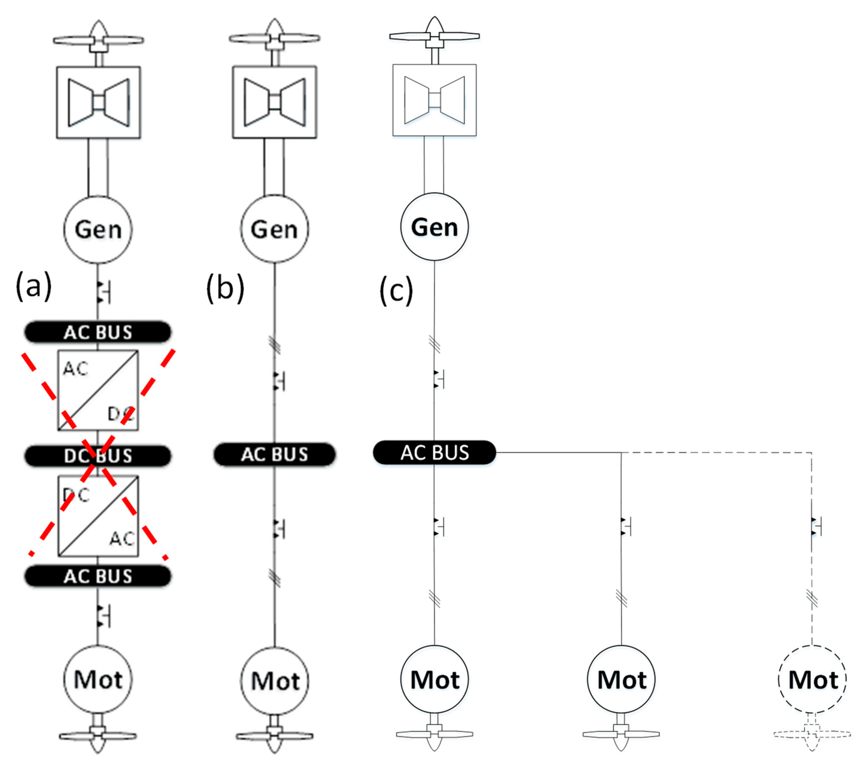
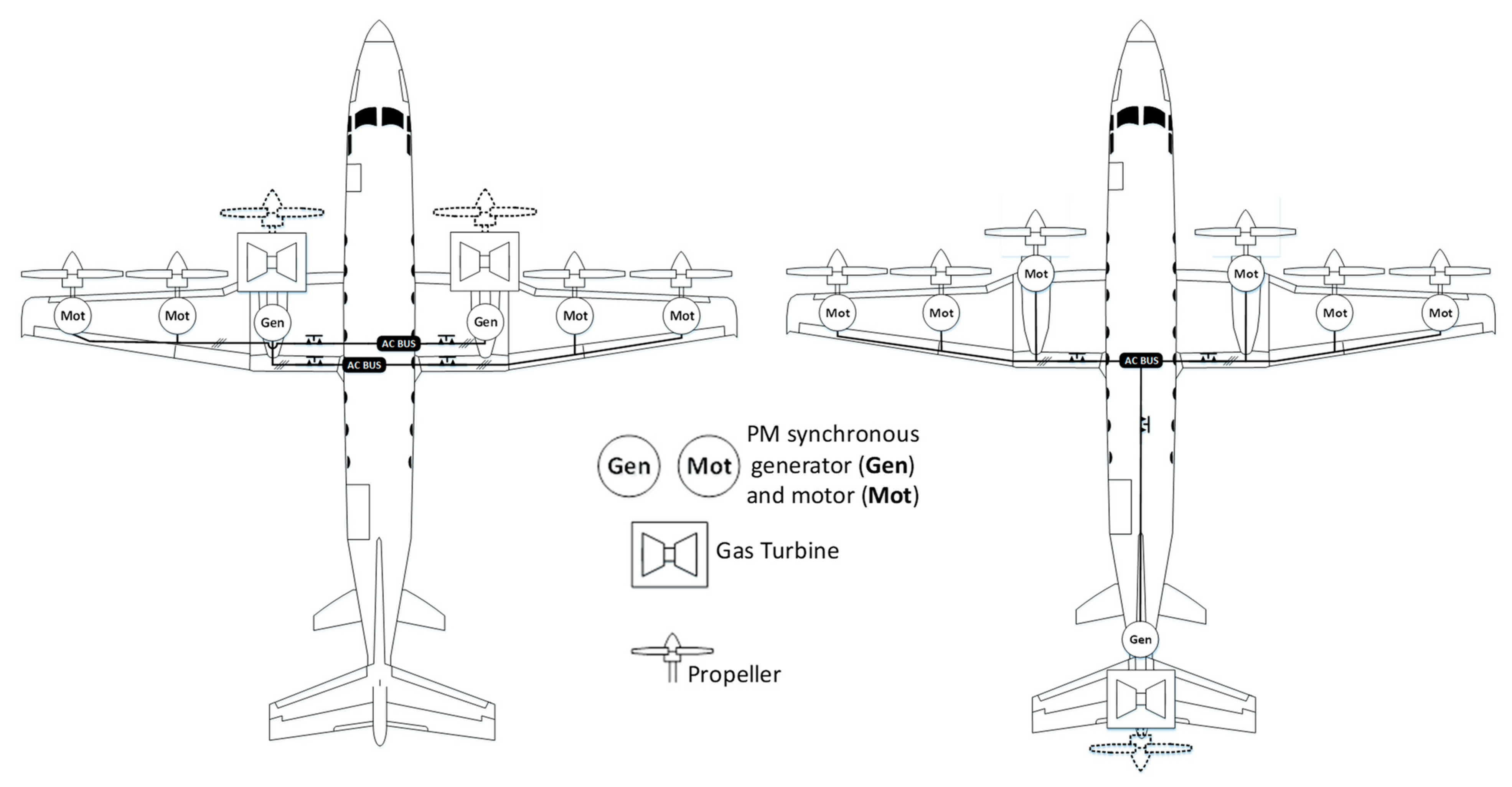
2. Context and Case Study of a “Power Electronic-Less” Powertrain for Aircraft Propulsion

Based on the previous state-of-the-art analysis, it has appeared that most of the propulsive architectures in more electric (hybrid or full electric) aircrafts are based on power electronics with a coupling between power sources and propulsion device through a DC bus, as illustrated in Figure 1a. The main idea of this paper is then to suppress this DC bus and these power electronics by directly connecting power sources (generators) to propulsive devices (motors) through a dedicated AC bus, as illustrated in the Figure 1b (for single motor connection) and Figure 1c (for multi-motor connection). All electric machines considered in that study are surface mounted PMSMs.

It could be said that the interaction between synchronous machines is a subject already considered in the context of large terrestrial networks and addressed by reference works as proposed by Kundur in [31]. However, some differences appear between this last approach and the one proposed in this paper. Indeed, Kundur has focused his work on ground transport networks of electricity, where large distances (long cables) are involved, which differs from the aeronautical application case which reactances are only composed of electrical machine reactances. Moreover, while the reference work [31] focuses only on the electrical dimension of the device, we aim here to also couple the mechanical dimension of the system, which is of major importance in terms of dynamics (stability).

In the “power electronic-less” structure of Figure 1b,c, considering the direct connection of the synchronous generator and the motors, obviously all machines operate at the same electrical speed (in a steady-state situation). Only two mechanical controls exist, each one on a system side: on the generator side, the mechanical speed, thus the AC link frequency, is controlled through the gas turbine, which manages the mechanical operation of this system. Oppositely, on the propeller sides, a pitch control of blades would be necessary to manage the aircraft thrust given the rotation speed operation. However, this latter issue is not the aim of our contribution.

This study may be applied to a wide spectrum of aeronautic applications. Two examples of topologies with six propellers are presented below, depending on whether one or more generators are placed on the wings in a series parallel architecture (Figure 2 left) or at the aircraft rear in the case of a series architecture (Figure 2 right).

Such electric distributed propulsion may offer aerodynamic advantages as studied in [10,11].

3. Modelling, Analysis Tools and Experimental Support for Stability Analysis

This section aims at defining the models and tools dedicated to the stability analysis of the powertrain. Three analysis means are successively proposed:

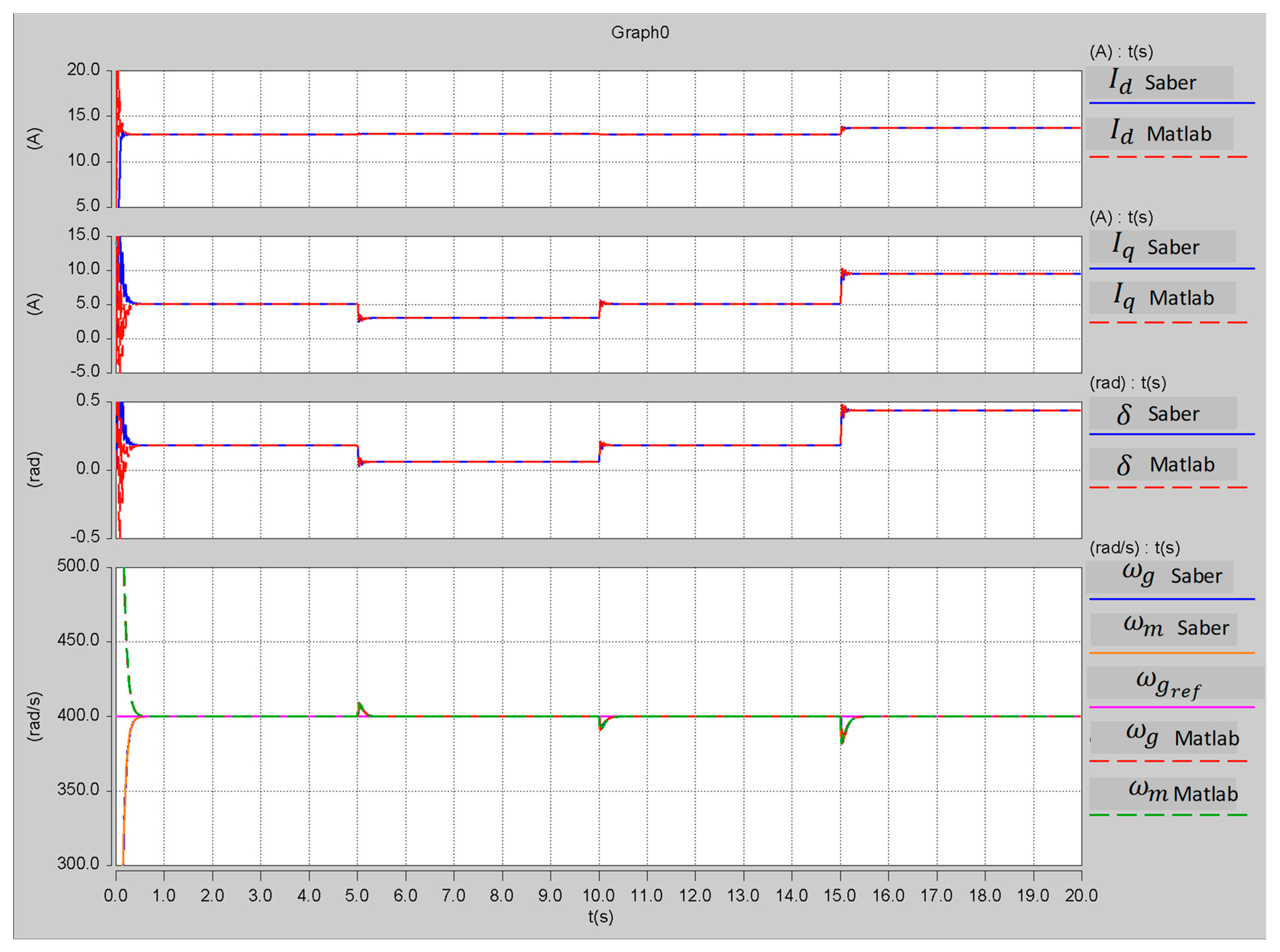
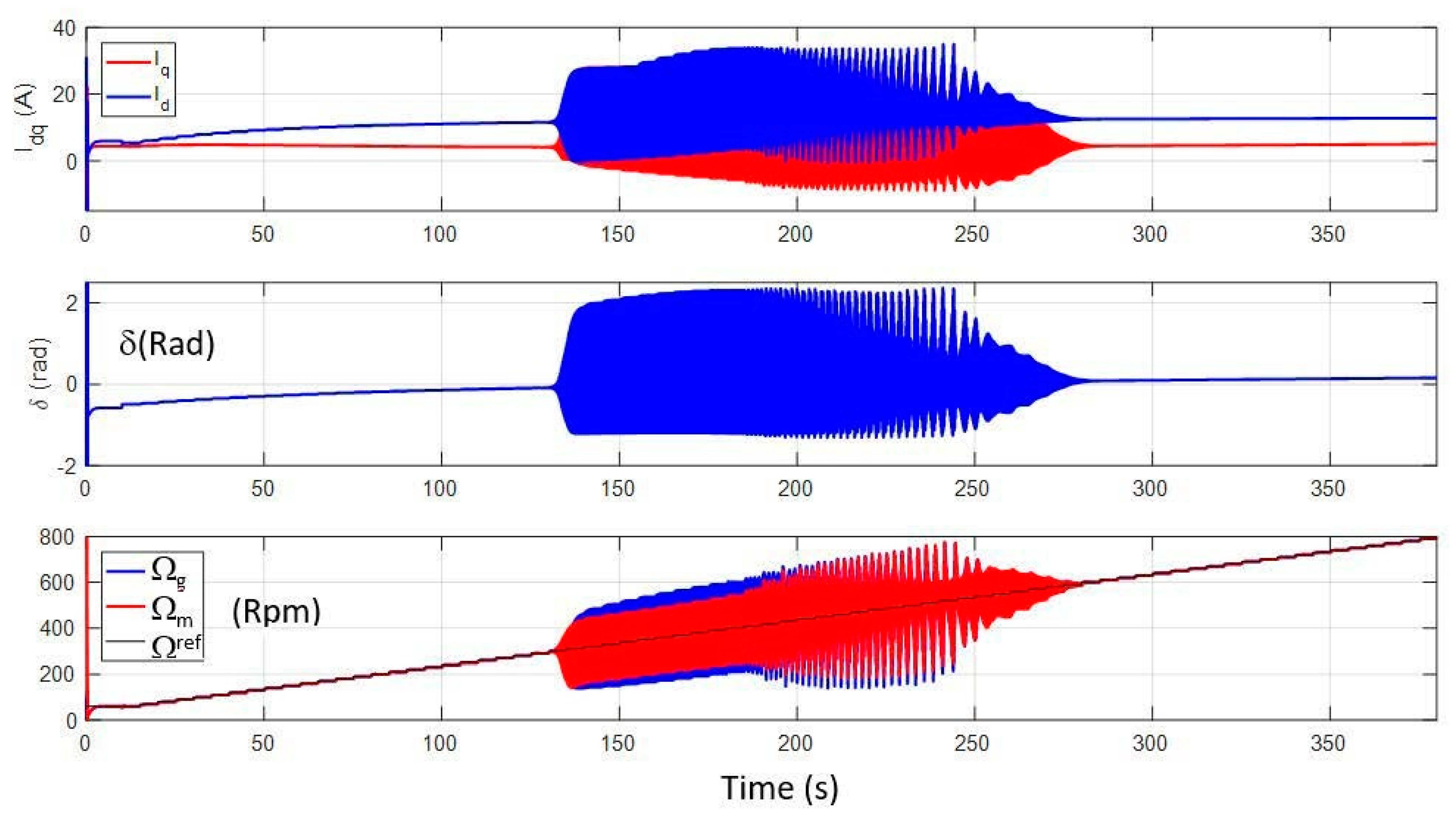
• First, a nonlinear state model is built, representing the transient behavior of the system. This analytic state model can be simulated in the time domain on Matlab Simulink and is compared for validation with another time simulation based on the Saber circuit solver [32].
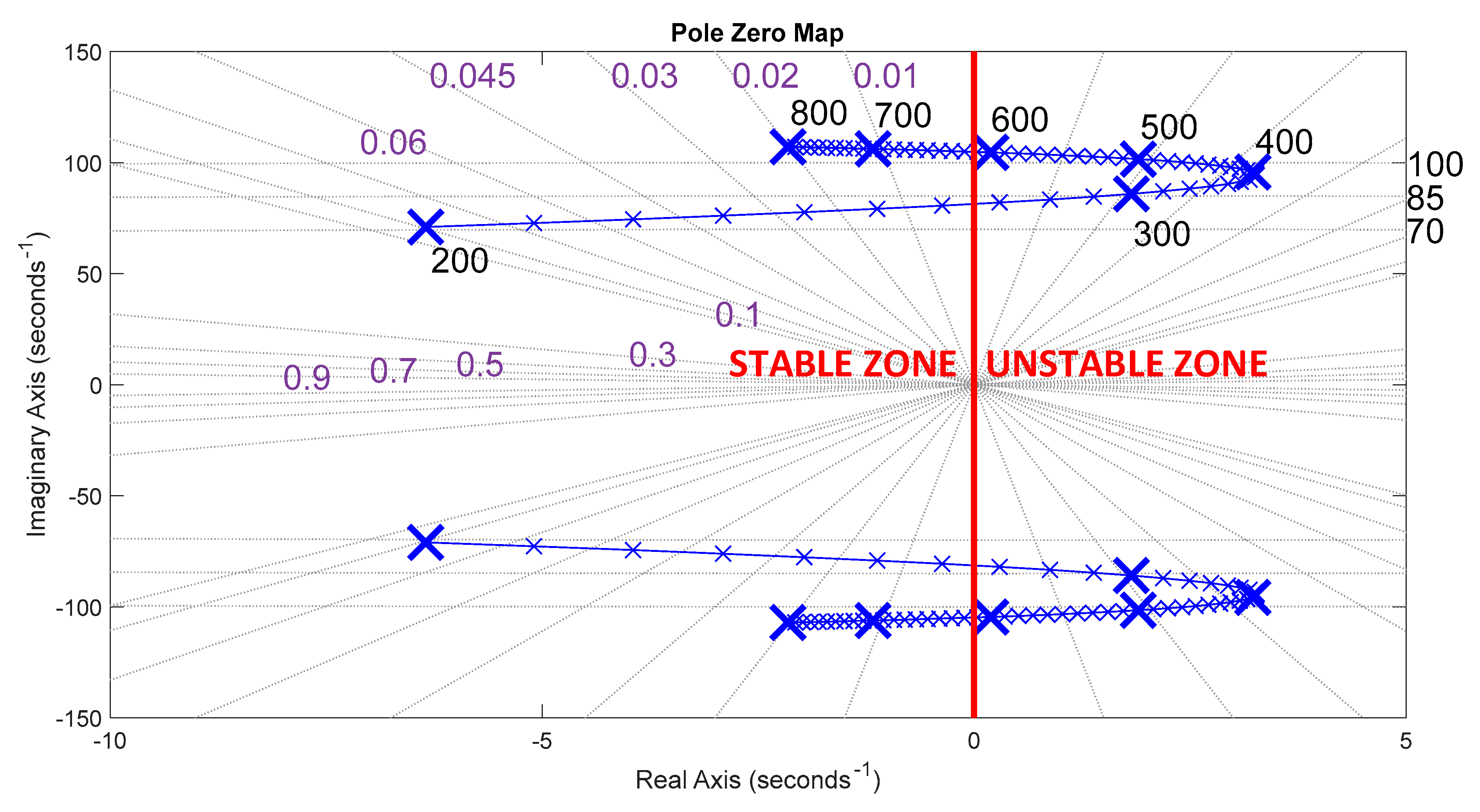
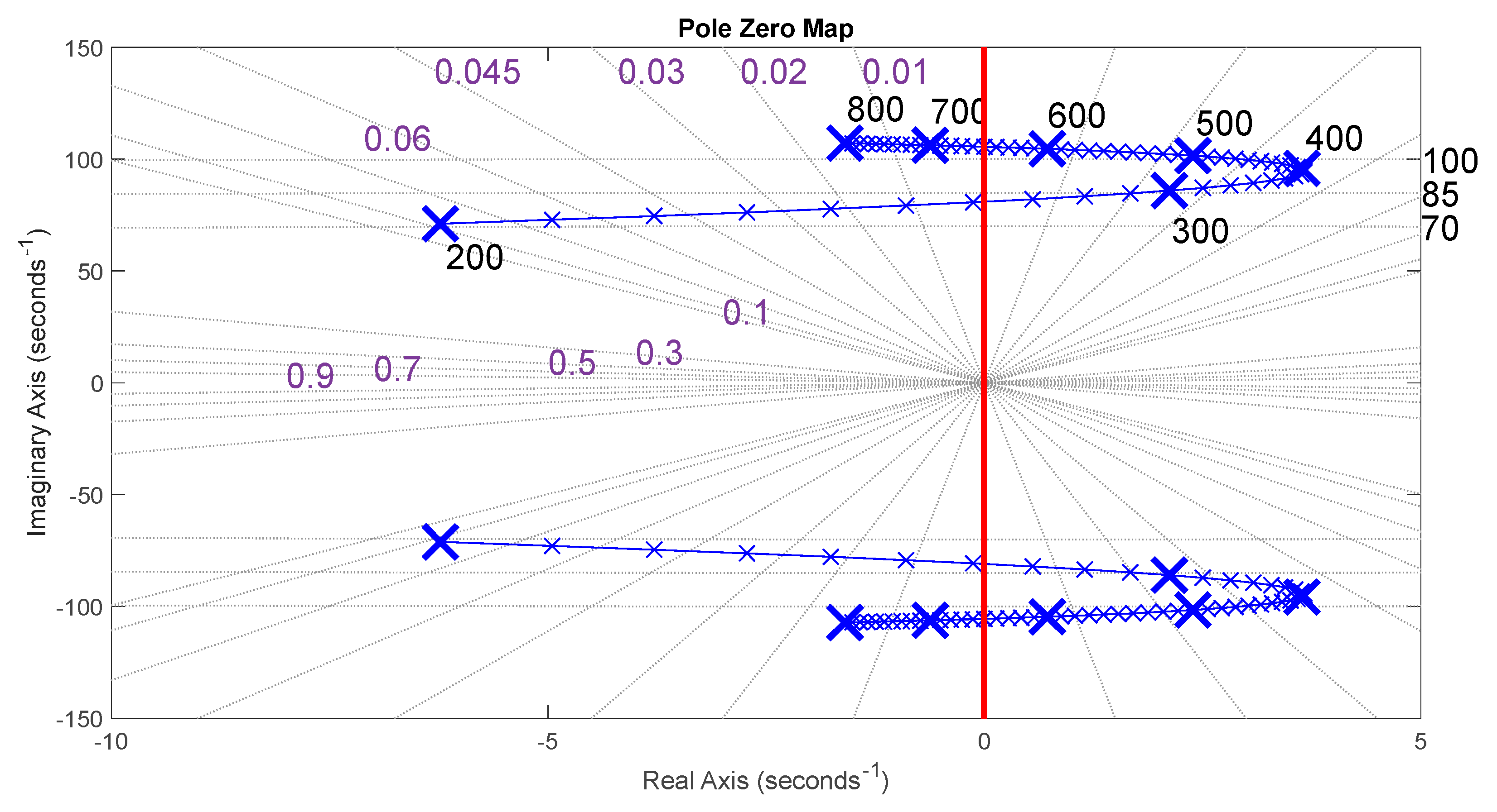
• Second, the previous analytic nonlinear state model can be small-signal linearized to set the root locus of the powertrain, in order to characterize the stability domain.
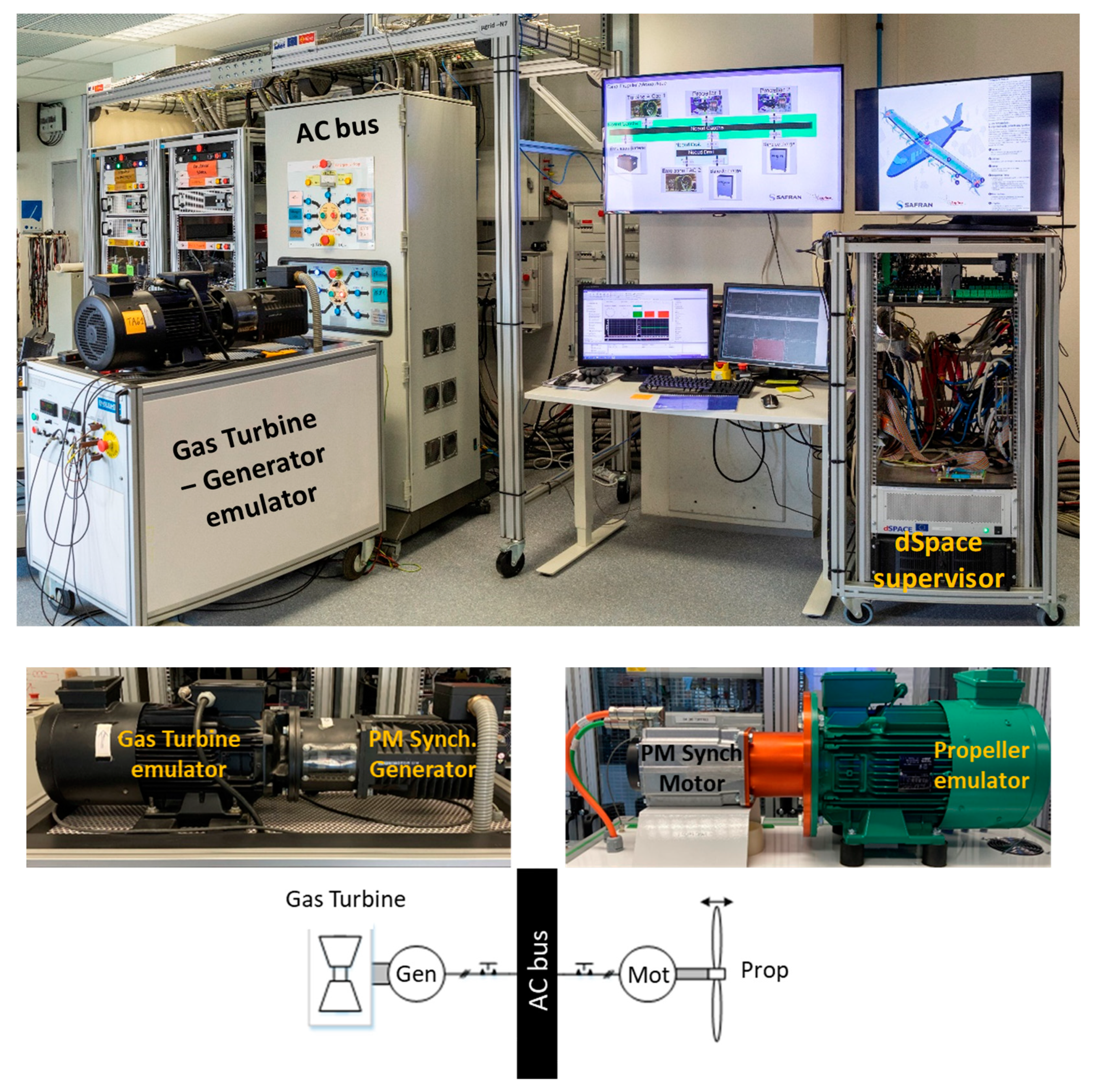
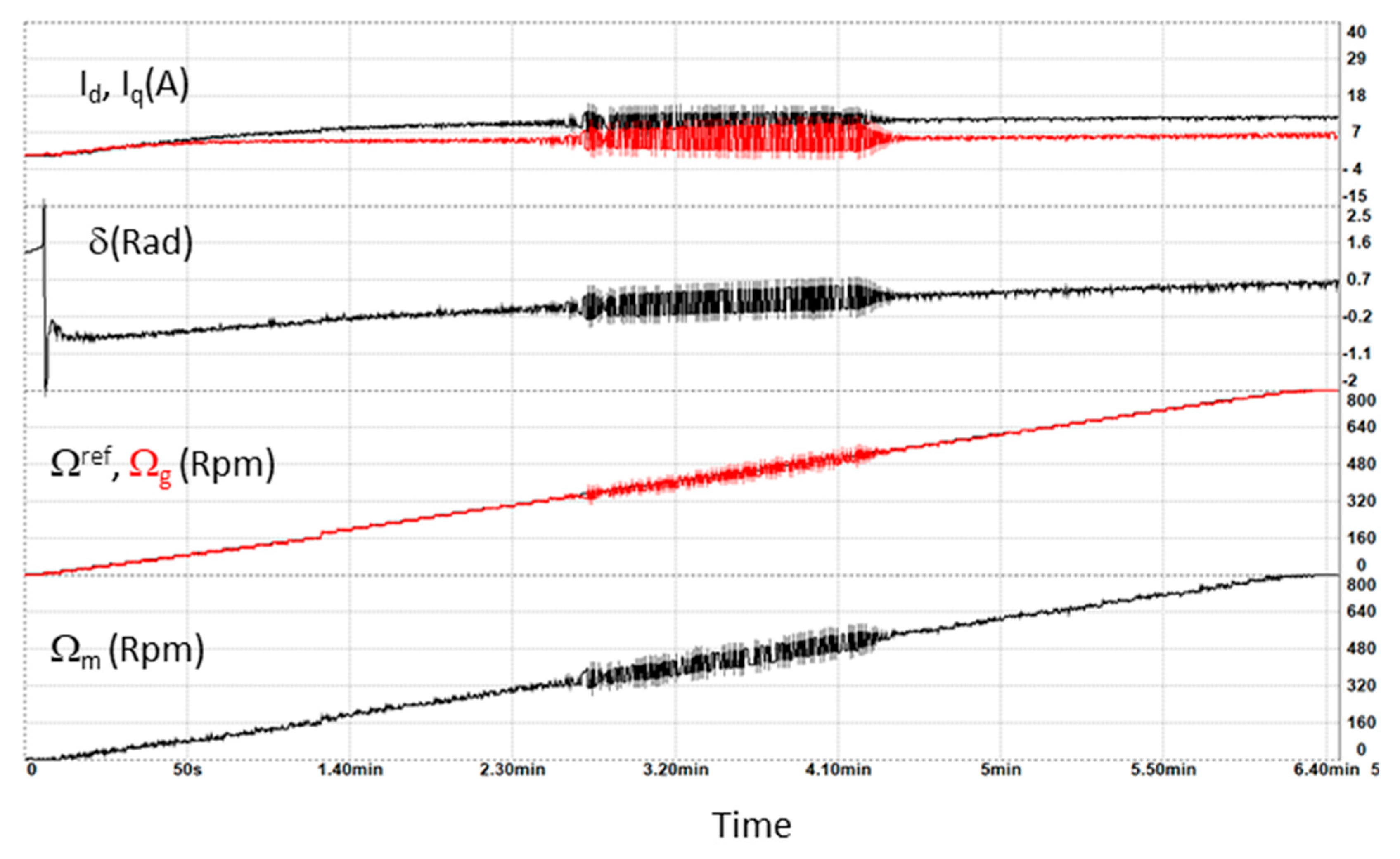
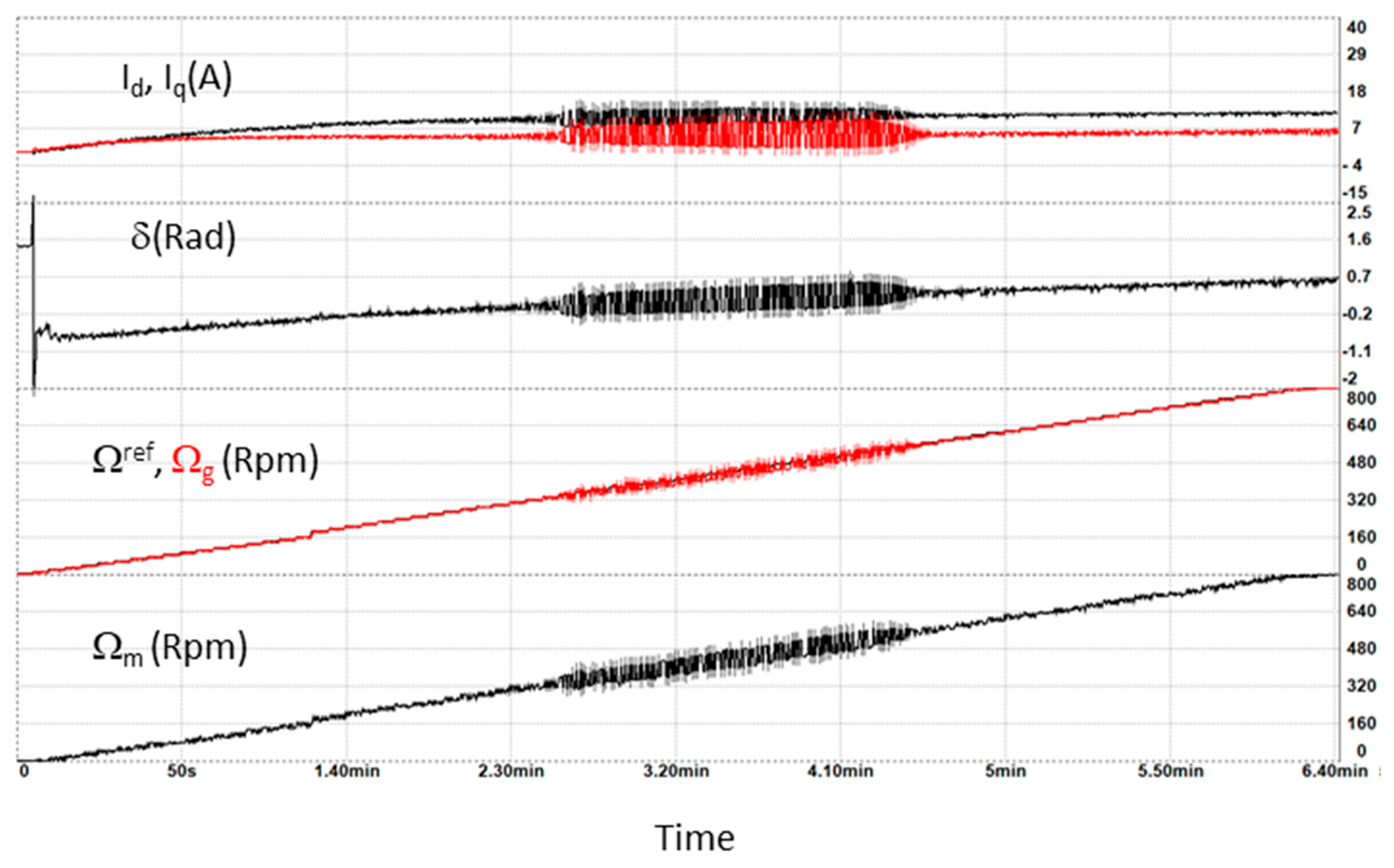
• Finally, a reduced power scale test bench was developed in order to validate theoretical analysis set from both previous approaches.

3.1. Nonlinear Analytic State Model

3.1.1. State Model Derivation

The analytic derivation for the generator and for the motor(s) is based on a Park’s model, which depends on the topology, which may be either single- (Figure 1b) or multi-motor (Figure 1c).

Each electric machine (generator or motor) is classically modelled by a Park’s (d,q) model that links the q axis with the electromotive force (emf): E_x = E_xq as illustrated in Figure 3 in which a generator and a motor are respectively represented in the (d_g,q_g) and (d_m,q_m) rotating reference frames.

In the case of a direct AC coupling of both machines (Figure 1b), the emfs can be phase shifted by the angle δ.

Let us note that this derivation may be generalized for a multi-motor topology, in which each electric motor (M_x) would have its own reference frame (d_mx,q_mx) with a δ_x phase shift with the generator. In order to represent the direct coupling between the generator and the motor(s) and to generalize the model derivation whatever the number of motors, it was chosen to represent all machines in the generator reference frame (d_g,q_g). In the rest of the paper, only a single-motor topology will be considered in order to simplify the stability analysis which remains complex even with that simplification. However, most of the theoretical consideration proposed in the next section remain relevant for multi-motor topology.

The Park’s model of a generator (1) and single-motor (2) association can be derived, where bold type is used to highlight vector or matrix variables as opposed to scalar quantities:

$$\begin{array}{c}{\mathit{V}}_{\mathit{d}\mathit{q}\mathbf{0}}^{\mathit{g}}=-\left(R_g\ast {\mathit{I}}_{\mathbf{3}}\right)·{\mathit{I}}_{\mathit{d}\mathit{q}\mathbf{0}}^{\mathit{g}}+{\displaystyle \frac{d}{dt}}\left({\Phi }_g{}_{\mathit{d}\mathit{q}\mathbf{0}}^{\mathit{g}}\right)+{\omega }_g\ast \left(\begin{array}{ccc}0& -1& 0\\ 1& 0& 0\\ 0& 0& 0\end{array}\right)·{\Phi }_g{}_{\mathit{d}\mathit{q}\mathbf{0}}^{\mathit{g}} \\ {\Phi }_g{}_{\mathit{d}\mathit{q}\mathbf{0}}^{\mathit{g}}=-L_g·{\mathit{I}}_{\mathit{d}\mathit{q}\mathbf{0}}^{\mathit{g}}+{\varphi }_{a_g}\ast \left(\begin{array}{c}1\\ 0\\ 0\end{array}\right)\end{array}$$

(1)

$$\begin{array}{c}{\mathit{V}}_{\mathit{d}\mathit{q}\mathbf{0}}^{\mathit{g}}=\left(R_m\ast {\mathit{I}}_{\mathbf{3}}\right)·I_{dq0}^g+{\displaystyle \frac{d}{dt}}\left({\Phi }_m{}_{\mathit{d}\mathit{q}\mathbf{0}}^{\mathit{g}}\right)+{\omega }_g\ast \left(\begin{array}{ccc}0& -1& 0\\ 1& 0& 0\\ 0& 0& 0\end{array}\right)·{\Phi }_m{}_{\mathit{d}\mathit{q}\mathbf{0}}^{\mathit{g}}\\ {\Phi }_m{}_{\mathit{d}\mathit{q}\mathbf{0}}^{\mathit{g}}=L_m·{\mathit{I}}_{\mathit{d}\mathit{q}\mathbf{0}}^{\mathit{g}}+{\varphi }_{a_m}\ast \left(\begin{array}{c}\cos \left(\delta \right)\\ -\sin \left(\delta \right)\\ 0\end{array}\right)\end{array}$$

(2)

$$\delta ={\theta }_g-{\theta }_m; \frac{d}{dt}\delta =\frac{d}{dt}\left({\theta }_g-{\theta }_m\right)={\omega }_g-{\omega }_m$$

(3)

where I₃ is the third order identity matrix, $R_g$, $R_m$,$L_g$, $L_m$, ${\varphi }_{a_g}$ and ${\varphi }_{a_m}$ are, respectively, the generator and motor resistances, inductances and rotor (magnet) fluxes. ${\theta }_g$,${\theta }_m$, ${\omega }_g \mathrm{and} {\omega }_m$, respectively, denote the generator and motor electric positions and angular speeds, $\delta$ being the electric angle that represents the phase shift between both machine frames.

When both machines are directly connected through an AC bus, the equality of stator voltages (${\mathit{V}}_{\mathit{d}\mathit{q}\mathbf{0}}^{\mathit{g}}$) leads to the final analytic model of the association that can be derived as a non-linear state model:

$$\frac{d}{dt}\left(\begin{array}{c}{I}_d^g\\ I_q^g\\ \delta \end{array}\right)=\left(\begin{array}{ccc}-\frac{\left(R_g+R_m\right)}{\left(L_g+L_m\right)}& {\omega }_g& 0\\ -{\omega }_g& -\frac{\left(R_g+R_m\right)}{\left(L_g+L_m\right)}& 0\\ 0& 0& 0\end{array}\right)\left(\begin{array}{c}{I}_d^g\\ I_q^g\\ \delta \end{array}\right)+\left(\begin{array}{cc}-\frac{{\varphi }_{a_m}\sin \left(\delta \right) }{L_g+L_m}& 0\\ -\frac{{\varphi }_{a_m}\cos \left(\delta \right) }{L_g+L_m}& \frac{{\varphi }_{a_g}}{L_g+L_m}\\ -1& 1\end{array}\right)\left(\begin{array}{c}{\omega }_m\\ {\omega }_g\end{array}\right)$$

(4)

where $I_d^g$, $I_q^g$ are the stator currents that have become common to both generator and motor after the direct AC connexion. The variables in red illustrate the model non linearities inside this state matrix form.

The torques are also derived for both machines by taking account of the total flux derivation for the generator (${\Phi }_g{}_{\mathit{d}\mathit{q}\mathbf{0}}^{\mathit{g}}$) and the motor (${\Phi }_m{}_{\mathit{d}\mathit{q}\mathbf{0}}^{\mathit{g}}$), respectively described in Equations (1) and (2):

$$T_{{em}_g}=\frac{3p_g}{2}\left({\Phi }_{g_d}^g·I_q^g-{\Phi }_{g_q}^g·I_d^g\right)=\frac{3p_g}{2}{\varphi }_{a_g}·I_q$$

(5)

$$T_{{em}_m}=\frac{3p_m}{2}\left({\Phi }_{m_d}^g·I_q^g-{\Phi }_{m_q}^g·I_d^g\right)==\frac{3p_m}{2}{\varphi }_{a_m}·\left(I_{d}sin\left(\delta \right)+I_{q}cos\left(\delta \right)\right)$$

(6)

where $p_g$ and $p_m$ are the number of pole pairs, respectively, for the generator and motor.

In the previous equations and for the rest of the derivation, the currents in the generator reference frame are simply denoted as the Park’s currents ($I_d^g$ = $I_d^{}$, $I_q^g=I_q^{}$).

The mechanical equations at both (generator and motor) sides have to be added to complete the state model:

$$\frac{d}{dt}{\omega }_g=\frac{p_g}{J_{e{q}_g}}\left(T_{TAG}-T_{e{m}_g}\right)-\frac{f_g}{J_{e{q}_g}}{\omega }_g with J_{e{q}_g}=J_g+J_{TAG} and {\omega }_g=p_g.{\mathsf{\Omega }}_g$$

(7)

$$\begin{array}{c}\frac{d}{dt}{\omega }_m=\frac{p_m}{J_{e{q}_m}}\left(T_{e{m}_m}-T_{pro{p}_m}\right)-\frac{f_m}{J_{e{q}_m}}{\omega }_m with J_{e{q}_m}=J_m+J_{prop} \\ and {\omega }_m=p_m.{\mathsf{\Omega }}_m\end{array}$$

(8)

where $T_{TAG}$ and $T_{e{m}_g}$ are, respectively, the gas turbine and the generator electromagnetic torques. $T_{prop}$ and $T_{e{m}_m}$ are, respectively, the propeller (load) and the motor electromagnetic torques. $J_g, J_{TAG}$, $J_m,J_{prop}$ are, respectively, the generator, gas turbine, motor and propeller moment of inertia. The two previous equations also describe the link between electric angular speeds ω_x and rotation mechanical speeds Ω_x.

The complete 5th order analytic state model with gas turbine and propeller torques as inputs is then obtained:

$$\frac{d}{dt}\left(\begin{array}{c}\begin{array}{c}\begin{array}{c}{I}_d\\ \begin{array}{c}\begin{array}{c}\begin{array}{c}\\ \end{array}\\ \end{array}\\ \begin{array}{c}{I}_q\\ \end{array}\end{array}\end{array}\\ \begin{array}{c}\begin{array}{c}\\ \delta \end{array}\\ \begin{array}{c}\begin{array}{c}\\ \begin{array}{c}\\ \begin{array}{c}\\ \begin{array}{c}{\omega }_m\\ \end{array}\end{array}\end{array}\end{array}\\ \end{array}\end{array}\end{array}\\ {\omega }_g\\ \end{array}\right)=\left(\begin{array}{c}\begin{array}{c}\begin{array}{c}\begin{array}{c}-\frac{R_g+R_m}{L_g+L_m}\\ \begin{array}{c}\begin{array}{c}\\ -{\omega }_g\end{array}\\ \end{array}\end{array}\\ \end{array}\\ 0\end{array}\\ \begin{array}{c}\\ \end{array}\\ \begin{array}{c}\begin{array}{c}\frac{3p_m^2}{2J_{e{q}_m}}{\varphi }_{a_m}\sin \left(\delta \right)\\ \begin{array}{c}\\ \begin{array}{c}\\ 0\end{array}\end{array}\end{array}\\ \end{array}\end{array}\begin{array}{c}\begin{array}{c}\begin{array}{c}\\ {\omega }_g\end{array}\\ \begin{array}{c}\begin{array}{c}\\ -\frac{R_g+R_m}{L_g+L_m}\end{array}\\ \begin{array}{c}\\ 0\end{array}\end{array}\end{array}\\ \begin{array}{c}\\ \end{array}\\ \begin{array}{c}\begin{array}{c}\frac{3p_m^2}{2J_{e{q}_m}}{\varphi }_{a_m}\cos \left(\delta \right)\\ \end{array}\\ -\frac{3p_g^2}{2J_{e{q}_g}}{\varphi }_{a_g}\end{array}\end{array} \begin{array}{c}\begin{array}{c}\begin{array}{c}0\\ \begin{array}{c}\begin{array}{c}\\ \end{array}\\ \begin{array}{c}0\\ \end{array}\end{array}\end{array}\\ \begin{array}{c}\begin{array}{c}\\ 0\end{array}\\ \begin{array}{c}\begin{array}{c}\\ \begin{array}{c}\\ \end{array}\end{array}\\ 0\end{array}\end{array}\end{array}\\ \begin{array}{c}\\ \end{array}\\ \begin{array}{c}\\ 0\end{array}\end{array} \begin{array}{c}\begin{array}{c}\begin{array}{c}-\frac{{\varphi }_{a_m}\sin \left(\delta \right)}{L_g+L_m}\\ \begin{array}{c}\\ -\frac{{\varphi }_{a_m}\cos \left(\delta \right)}{L_g+L_m}\end{array}\end{array}\\ \begin{array}{c}\\ \begin{array}{c}-1\\ \begin{array}{c}\\ \begin{array}{c}\begin{array}{c}\\ \frac{-f_m}{J_{e{q}_m}}\end{array}\\ \begin{array}{c}\\ \end{array}\end{array}\end{array}\end{array}\end{array}\end{array}\\ 0\\ \end{array} \begin{array}{c}\begin{array}{c}\begin{array}{c}\begin{array}{c}0\\ \end{array}\\ \end{array}\\ \begin{array}{c}\frac{{\varphi }_{a_g}}{L_g+L_m}\\ \begin{array}{c}\begin{array}{c}\\ 1\end{array}\\ \begin{array}{c}\\ \begin{array}{c}\begin{array}{c}\\ \end{array}\\ 0\end{array}\end{array}\end{array}\end{array}\end{array}\\ \\ \frac{-f_g}{J_{e{q}_g}}\end{array}\right)\left(\begin{array}{c}\begin{array}{c}\begin{array}{c}{I}_d\\ \begin{array}{c}\begin{array}{c}\begin{array}{c}\\ \end{array}\\ \end{array}\\ \begin{array}{c}{I}_q\\ \end{array}\end{array}\end{array}\\ \begin{array}{c}\begin{array}{c}\\ \delta \end{array}\\ \begin{array}{c}\begin{array}{c}\\ \begin{array}{c}\\ \begin{array}{c}\\ \begin{array}{c}{\omega }_m\\ \end{array}\end{array}\end{array}\end{array}\\ \end{array}\end{array}\end{array}\\ {\omega }_g\\ \end{array}\right)+\left(\begin{array}{c}\begin{array}{c}\begin{array}{c}\\ \begin{array}{c}0\\ \begin{array}{c}\\ \end{array}\end{array}\end{array}\\ \begin{array}{c}\\ \begin{array}{c}\begin{array}{c}0\\ \begin{array}{c}\\ \begin{array}{c}\\ 0\end{array}\end{array}\end{array}\\ \end{array}\end{array}\end{array}\\ \begin{array}{c}\\ 0\end{array}\\ \begin{array}{c}\begin{array}{c}\\ \begin{array}{c}\\ \frac{p_g}{J_{e{q}_g}}\end{array}\end{array}\\ \end{array}\end{array}\begin{array}{c}\begin{array}{c}\begin{array}{c}\\ \begin{array}{c}0\\ \begin{array}{c}\\ \end{array}\end{array}\end{array}\\ \begin{array}{c}\\ \begin{array}{c}\begin{array}{c}0\\ \begin{array}{c}\\ \begin{array}{c}\\ 0\end{array}\end{array}\end{array}\\ \end{array}\end{array}\end{array}\\ \begin{array}{c}\\ -\frac{p_m}{J_{e{q}_m}}\end{array}\\ \begin{array}{c}\begin{array}{c}\\ \begin{array}{c}0\\ \end{array}\end{array}\\ \end{array}\end{array}\right)\left(\begin{array}{c}{T}_{TAG}\\ T_{pro{p}_m}\end{array}\right)$$

(9)

Actually, the gas turbine is classically controlled to drive its rotation speed. Thus, the speed control of the gas turbine—generator association can be added to complete the model. In our study, as shown on Figure 4, an integral proportional (IP) controller structure was retained:

This control structure sets an additional state equation which links the gas turbine torque $T_{TAG}$ and the reference generator speed ${\omega }_{g_{ref}}$ which becomes the new system input:

$$\begin{array}{c}\frac{d{T}_{TAG}}{dt}=\frac{k_{IP}}{T_{IP}}\ast \frac{{\omega }_{g_{ref}}}{p_g}-\frac{k_{IP}}{T_{IP}}\ast \frac{{\omega }_g}{p_g}-\frac{k_{IP}}{p_g} \ast \frac{d{\omega }_g}{dt}\\ =\frac{k_{IP}}{T_{IP}}\ast \frac{{\omega }_{g_{ref}}}{p_g}-\frac{k_{IP}}{T_{IP}}\ast \frac{{\omega }_g}{p_g}-\frac{k_{IP}}{p_g} \ast \frac{p_g}{J_{e{q}_g}}\left(T_{TAG}-T_{e{m}_g}\right)+\frac{k_{IP}}{p_g}\ast \frac{f}{J_{e{q}_g}}{\omega }_g\end{array}$$

(10)

where: ${\omega }_{g_{ref}}$ = $p_g\ast {\mathsf{\Omega }}_{g_{ref}}$

Finally, a sixth order analytic state model can be derived, where the generator reference speed and the propeller load torque become the new inputs:

$$\frac{d}{dt}\left(\begin{array}{c}\begin{array}{c}\begin{array}{c}\\ \begin{array}{c}\begin{array}{c}\begin{array}{c}\\ I_d\end{array}\\ \end{array}\\ \begin{array}{c}\\ I_q\end{array}\end{array}\end{array}\\ \begin{array}{c}\begin{array}{c}\\ \delta \end{array}\\ \begin{array}{c}\begin{array}{c}\\ \begin{array}{c}\\ \begin{array}{c}\\ \begin{array}{c}{\omega }_m\\ \end{array}\end{array}\end{array}\end{array}\\ {\omega }_g\end{array}\end{array}\end{array}\\ \begin{array}{c}\\ T_{TAG}\end{array}\\ \begin{array}{c}\\ \end{array}\end{array}\right)=\left(\begin{array}{c}\begin{array}{c}\begin{array}{c}\begin{array}{c}-\frac{R_g+R_m}{L_g+L_m}\\ \begin{array}{c}\begin{array}{c}\begin{array}{c}\\ -{\omega }_g\end{array}\\ \end{array}\\ \end{array}\end{array}\\ 0\end{array}\\ \end{array}\\ \frac{3p_m^2}{2J_{e{q}_m}}{\varphi }_{a_m}\sin \left(\delta \right)\\ \begin{array}{c}\begin{array}{c}\\ \begin{array}{c}0\\ \begin{array}{c}\begin{array}{c}\\ \end{array}\\ 0\end{array}\end{array}\end{array}\\ \end{array}\end{array}\begin{array}{c}\begin{array}{c}\begin{array}{c}{\omega }_g\\ \begin{array}{c}\\ \end{array}\end{array}\\ \begin{array}{c}\begin{array}{c}-\frac{R_g+R_m}{L_g+L_m}\\ \end{array}\\ 0\end{array}\end{array}\\ \begin{array}{c}\\ \frac{3p_m^2}{2J_{e{q}_m}}{\varphi }_{a_m}\cos \left(\delta \right)\end{array}\\ \begin{array}{c}\begin{array}{c}-\frac{3p_g^2}{2J_{e{q}_g}}{\varphi }_{a_g}\\ \end{array}\\ \frac{k_{IP}}{p_g}\left(\frac{3p_g^2}{2J_{e{q}_g}}{\varphi }_{a_g}\right)\end{array}\end{array}\begin{array}{c}\begin{array}{c}\begin{array}{c}0\\ \begin{array}{c}\\ \begin{array}{c}\\ 0\end{array}\end{array}\end{array}\\ \begin{array}{c}\begin{array}{c}\\ \end{array}\\ \begin{array}{c}\begin{array}{c}0\\ \begin{array}{c}\\ \begin{array}{c}\\ \begin{array}{c}0\\ \end{array}\end{array}\end{array}\end{array}\\ 0\end{array}\end{array}\end{array}\\ \begin{array}{c}\begin{array}{c}\\ \end{array}\\ \end{array}\\ 0\end{array} \begin{array}{c}\begin{array}{c}\begin{array}{c}-\frac{{\varphi }_{a_m}\sin \left(\delta \right)}{L_g+L_m}\\ \begin{array}{c}\\ -\frac{{\varphi }_{a_m}\cos \left(\delta \right)}{L_g+L_m}\end{array}\end{array}\\ \begin{array}{c}\\ \begin{array}{c}-1\\ \begin{array}{c}\\ \begin{array}{c}\begin{array}{c}\frac{-f_m}{J_{e{q}_m}}\\ \begin{array}{c}0\\ \end{array}\end{array}\\ \begin{array}{c}\\ \end{array}\end{array}\end{array}\end{array}\end{array}\end{array}\\ 0\\ \end{array} \begin{array}{c}\begin{array}{c}\begin{array}{c}0\\ \end{array}\\ \begin{array}{c}\\ \begin{array}{c}\begin{array}{c}\frac{{\varphi }_{a_g}}{L_g+L_m}\\ \end{array}\\ \begin{array}{c}1\\ \begin{array}{c}\begin{array}{c}\\ 0\end{array}\\ \end{array}\end{array}\end{array}\end{array}\end{array}\\ \frac{-f_g}{J_{e{q}_g}}\\ \begin{array}{c}\\ -\frac{k_{IP}}{p_g}\left(\frac{1}{T_{IP}}-\frac{f}{J_{e{q}_g}}\right)\end{array}\end{array} \begin{array}{c}\begin{array}{c}\begin{array}{c}0\\ \begin{array}{c}\\ \begin{array}{c}\\ \end{array}\end{array}\end{array}\\ \begin{array}{c}0\\ \begin{array}{c}\begin{array}{c}\\ \begin{array}{c}\\ \begin{array}{c}0\\ \end{array}\end{array}\end{array}\\ 0\end{array}\end{array}\end{array}\\ \begin{array}{c}\\ \frac{p_g}{J_{e{q}_g}}\end{array}\\ \begin{array}{c}\\ \frac{-k_{IP}}{J_{e{q}_g}}\end{array}\end{array}\right)\left(\begin{array}{c}\begin{array}{c}\begin{array}{c}\\ \begin{array}{c}\begin{array}{c}\begin{array}{c}\\ I_d\end{array}\\ \end{array}\\ \begin{array}{c}\\ I_q\end{array}\end{array}\end{array}\\ \begin{array}{c}\begin{array}{c}\\ \delta \end{array}\\ \begin{array}{c}\begin{array}{c}\\ \begin{array}{c}\\ \begin{array}{c}\\ \begin{array}{c}{\omega }_m\\ \end{array}\end{array}\end{array}\end{array}\\ {\omega }_g\end{array}\end{array}\end{array}\\ \begin{array}{c}\\ T_{TAG}\end{array}\\ \begin{array}{c}\\ \end{array}\end{array}\right)+\left(\begin{array}{c}\begin{array}{c}\begin{array}{c}0\\ \begin{array}{c}\\ \begin{array}{c}\\ \end{array}\end{array}\end{array}\\ \begin{array}{c}0\\ \begin{array}{c}\begin{array}{c}\\ \begin{array}{c}\\ \begin{array}{c}0\\ \end{array}\end{array}\end{array}\\ 0\end{array}\end{array}\end{array}\\ \begin{array}{c}\\ 0\end{array}\\ \begin{array}{c}\begin{array}{c}\\ \begin{array}{c}\\ \end{array}\end{array}\\ \frac{k_{IP}}{T_{IP}{p}_g}\end{array}\end{array}\begin{array}{c}\begin{array}{c}\begin{array}{c}0\\ \begin{array}{c}\\ \begin{array}{c}\\ \end{array}\end{array}\end{array}\\ \begin{array}{c}0\\ \begin{array}{c}\begin{array}{c}\\ \begin{array}{c}\\ \begin{array}{c}0\\ \end{array}\end{array}\end{array}\\ -\frac{p_m}{J_{e{q}_m}}\end{array}\end{array}\end{array}\\ \begin{array}{c}\\ 0\end{array}\\ \begin{array}{c}\begin{array}{c}\\ \begin{array}{c}\\ 0\end{array}\end{array}\\ \end{array}\end{array}\right)\left(\begin{array}{c}{\omega }_{g_{ref}}\\ T_{pro{p}_m}\end{array}\right)$$

(11)

In that model, the state matrix involves all nonlinearities of the powertrain (in red) with sine and cosine terms and also with bilinearities (products of two state variables).

Let us note that the same derivation process may be applied for a multi-motor association with n propellers, leading to an order extension of the state model:

$$\frac{d}{dt}\left(\begin{array}{c}\begin{array}{c}{I}_{d_1}\\ \begin{array}{c}{I}_{q_1}\\ I_{d_2}\\ I_{q_2}\\ ⋮\\ {\delta }_1\end{array}\\ \begin{array}{c}{\delta }_2\\ ⋮\end{array}\end{array}\\ \begin{array}{c}\begin{array}{c}{\omega }_1\\ {\omega }_2\\ ⋮\end{array}\\ {\omega }_g\\ T_{TAG}\end{array}\end{array}\right)=\mathit{A}·\left(\begin{array}{c}\begin{array}{c}{I}_{d_1}\\ \begin{array}{c}{I}_{q_1}\\ I_{d_2}\\ I_{q_2}\\ ⋮\\ {\delta }_1\end{array}\\ \begin{array}{c}{\delta }_2\\ ⋮\end{array}\end{array}\\ \begin{array}{c}\begin{array}{c}{\omega }_1\\ {\omega }_2\\ ⋮\end{array}\\ {\omega }_g\\ T_{TAG}\end{array}\end{array}\right)+\mathit{B}·\left(\begin{array}{c}{\omega }_{g_{ref}}\\ \begin{array}{c}{T}_{pro{p}_1}\\ T_{pro{p}_2}\\ \begin{array}{c}⋮\\ T_{pro{p}_n}\end{array}\end{array}\end{array}\right)$$

(12)

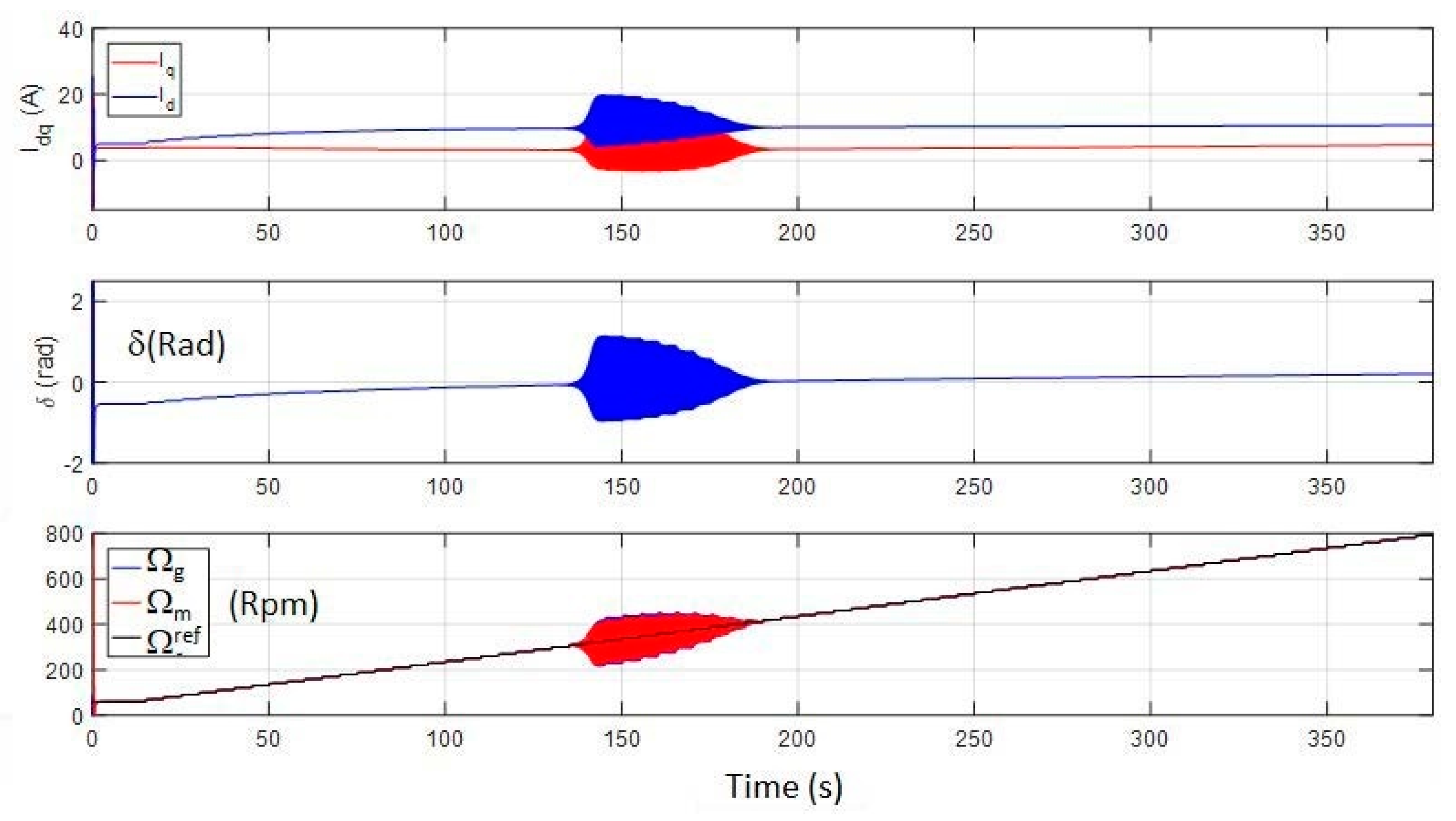
3.1.2. State Model Validation

In order to validate the previous state model, we have considered a circuit solver (Saber) that is seen here as a reference. In that circuit simulation, the synchronous machines (generator and motor) are modelled from proprietary models from Safran Tech including Park’s model. The relevance of such models has been proved in several previous studies. We consider here a single-motor association in which the topology is equivalent to the state model (11). The Saber circuit solver is then compared with the nonlinear state model (11) simulated on Matlab Simulink in the same operating conditions: the generator speed being controlled at constant speed, the powertrain has to face load torque steps successively at 5, 10 and 15 s. Figure 5 emphasizes the quasi-perfect accordance of both time simulations. Note that these simulations were obtained with a high bandwidth (3 Hz) for the gas turbine speed controller in order to ensure the system stability, this latter issue being under study in the next section. Note also that in the Figure 5, the initial conditions are set differently in Saber and in Matlab, just to satisfy the constraints specific to each solver: the initial transients are not to be considered for the analysis.

The previous simulation also emphasizes the capability of this system to face load torque variation on the propeller side. Indeed, in Figure 5, load torque variations are provoked at times 5 s, 10 s and 15 s and their consequences are visible on the displayed electric variables (I_d,q and δ) which remain stable despite the propeller torque transients. More generally, it was verified in our study that the system is capable to face transients on the propeller torque while the powertrain is in stable operation.

3.2. Small-Signal Linearization of the Analytic Model

Based on the previous (11) nonlinear state model, the aim of this section is to linearize the model in order to allow a simple characterization of the stability domain by means of the root locus of the powertrain. For that purpose, we have chosen here to derive a small-signal-state model linearized around steady-state operating points.

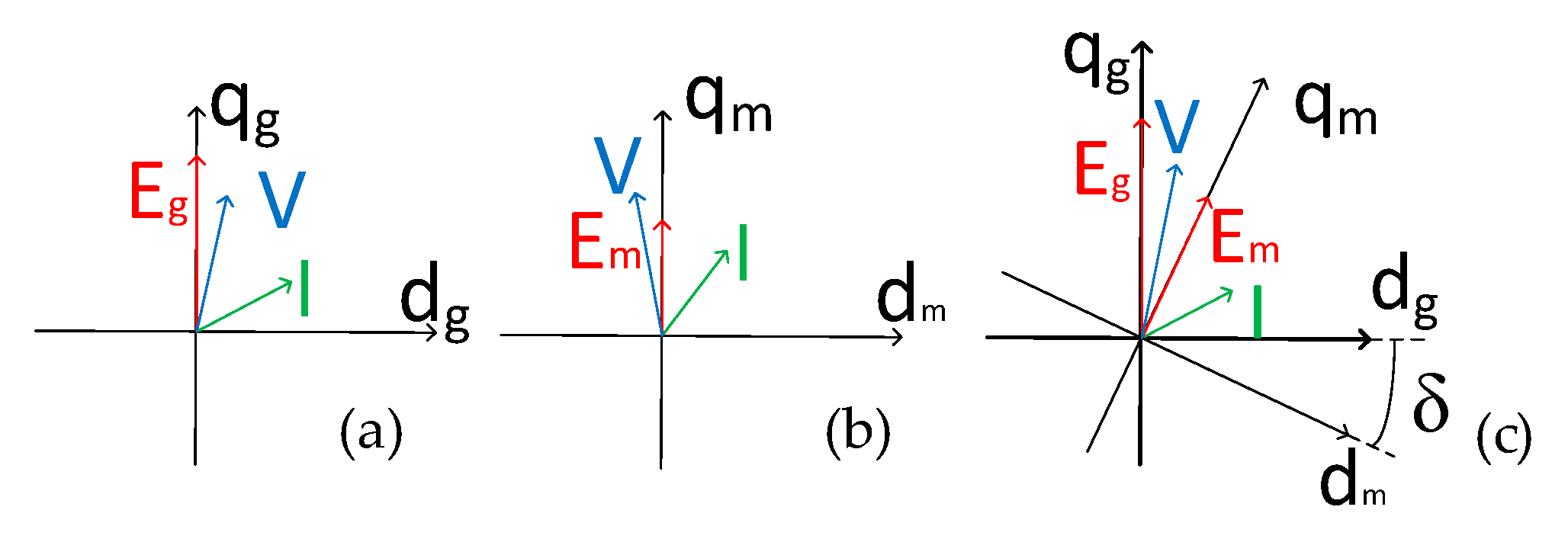
3.2.1. Steady-State Model Derivation

A preliminary step before linearizing the model is to calculate analytically all state variables at steady state for any operating conditions. Then, the small-signal linearization should be achieved around these steady-state points.

At steady state ($\frac{d}{dt}$ = 0), Equations (1) and (2) are:

$$\begin{array}{c}-\left(R_g\ast {\mathit{I}}_{\mathbf{3}}\right)·{\mathit{I}}_{\mathit{d}\mathit{q}\mathbf{0}}^{\mathit{g}}-\omega \ast \left(\begin{array}{ccc}0& -1& 0\\ 1& 0& 0\\ 0& 0& 0\end{array}\right)·L_g·{\mathit{I}}_{\mathit{d}\mathit{q}\mathbf{0}}^{\mathit{g}}+\omega \ast {\varphi }_{a_g}\left(\begin{array}{c}0\\ 1\\ 0\end{array}\right)=\\ \left(R_m\ast {\mathit{I}}_{\mathbf{3}}\right)·{\mathit{I}}_{\mathit{d}\mathit{q}\mathbf{0}}^{\mathit{g}}+\omega \ast \left(\begin{array}{ccc}0& -1& 0\\ 1& 0& 0\\ 0& 0& 0\end{array}\right)·L_m·{\mathit{I}}_{\mathit{d}\mathit{q}\mathbf{0}}^{\mathit{g}}+\omega \ast {\varphi }_{a_m}\left(\begin{array}{c}\sin \left(\delta \right)\\ \cos \left(\delta \right)\\ 0\end{array}\right)\end{array}$$

(13)

Equation (3), under steady-state condition, leads to the equality of angular speeds:

$$\frac{d}{dt}\delta = 0 \Rightarrow {\omega }_g = {\omega }_m = \omega$$

(14)

A simplified expression is given by deriving the electromotive forces of both machines:

$$\begin{array}{c}{E}_m\sin \left(\delta \right)=-\left(R_g+R_m\right)\ast I_d+\left(L_g+L_m\right)\ast \omega \ast I_q\\ E_m\cos \left(\delta \right)=-\left(R_g+R_m\right)\ast I_q-\left(L_g+L_m\right)\ast \omega \ast I_d+E_g\\ \mathrm{With} E_g=\omega ·{\varphi }_{a_g} \mathrm{et} E_m=\omega ·{\varphi }_{a_m}\hfill \end{array}$$

(15)

Solving analytically this system to calculate the steady-state variables ($I_d,I_q,\delta$) with respect to the inputs (${\omega }_{g_{ref}}$, $T_{pro{p}_m}$) is quite complicated and only the result is given here. The previous system (15) with two equations of two unknown variables ($I_d,I_q$) is solved by deriving a second order polynomial equation:

$$\begin{array}{c}\left({\left(\frac{\left(L_g+L_m\right)·\omega }{2}+\frac{{\left(R_g+R_m\right)}^2}{\left(L_g+L_m\right)}·\frac{1}{2\omega }\right)}^2+{\left(-\frac{\left(R_g+R_m\right)}{2}-\frac{{\left(L_g+L_m\right)}^2}{\left(R_g+R_m\right)}·\frac{{\omega }^2}{2}\right)}^2\right)·I_q^2+\\ 2\left[\begin{array}{c}\left(\frac{\left(L_g+L_m\right)·\omega }{2}+\frac{{\left(R_g+R_m\right)}^2}{\left(L_g+L_m\right)}·\frac{1}{2\omega }\right)·cste·\left(R_g+R_m\right)+\\ \left(-\frac{\left(R_g+R_m\right)}{2}-\frac{{\left(L_g+L_m\right)}^2}{\left(R_g+R_m\right)}·\frac{{\omega }^2}{2}\right)·\left(cste\left(L_g+L_m\right)·\omega +E_g\right)\end{array}\right]·I_q\\ +\left({\left(cste·\left(R_g+R_m\right)\right)}^2+{\left(cste·\left(L_g+L_m\right)·\omega +E_g\right)}^2-E_m^2\right)=0 \end{array}$$

(16)

With $cste=\left(\frac{\left(E_m^2-E_g^2\right)}{2E_g·\left(L_g+L_m\right)·\omega }+\frac{T_{pro{p}_m}}{3p_m}·\frac{\left(L_g+L_m\right)}{\left(R_g+R_m\right)}·\frac{1}{E_g}·\left(\frac{{\left(R_g+R_m\right)}^2}{{\left(L_g+L_m\right)}^2}+{\omega }^2\right)\right)$

$$\delta =\mathrm{asin}\left(\frac{\left(-\left(R_g+R_m\right)·I_d+\left(L_g+L_m\right)·\omega ·I_q\right)}{E_m}\right)$$

(17)

ω being replaced by its reference value, the steady-state operation of the powertrain can be derived from the inputs (${\omega }_{g_{ref}}$, $T_{pro{p}_m}$).

3.2.2. Linearized State Model Derivation

Each nonlinear variable X is linearized around its steady-state (SS) value: $X=X_{SS}+\Delta X$.

From the nonlinear state model (11) the linearization becomes:

$$\begin{array}{cc}\frac{d}{dt}\left(\begin{array}{c}\begin{array}{c}\Delta I_d\\ \Delta I_q\\ \Delta \delta \end{array}\\ \begin{array}{c}\Delta {\omega }_m\\ \Delta {\omega }_g\\ \Delta T_{TAG}\end{array}\end{array}\right)=& \left(\begin{array}{c}\begin{array}{c}-\frac{R_g+R_m}{L_g+L_m}\\ -{\omega }_{g_{SS}}\\ \begin{array}{c}0\\ \\ \frac{3p_m^2}{2J_{e{q}_m}}\left({\varphi }_{a_m}\sin \left({\delta }_{SS}\right)\right)\end{array}\end{array}\\ \begin{array}{c}\\ \begin{array}{c}0\\ \begin{array}{c}\\ \begin{array}{c}\\ 0\end{array}\end{array}\end{array}\\ \end{array}\end{array}\begin{array}{c}\begin{array}{c}{\omega }_{g_{SS}}\\ -\frac{R_g+R_m}{L_g+L_m}\\ 0\\ \end{array}\\ \begin{array}{c}\frac{3p_m^2}{2J_{e{q}_m}}\left({\varphi }_{a_m}\cos \left({\delta }_{SS}\right)\right)\\ \frac{-3p_g^2}{2J_{e{q}_g}}{\varphi }_{a_g}\\ \frac{\left(k_{IP}/p_g\right)3p_g^2}{2J_{e{q}_g}}{\varphi }_{a_g}\end{array}\end{array}\begin{array}{c}\begin{array}{c}-\frac{{\omega }_{m_{SS}}{\Phi }_{a_m}}{L_g+L_m}cos\left({\delta }_{SS}\right)\\ \frac{{\omega }_{m_{SS}}{\Phi }_{a_m}}{L_g+L_m}sin\left({\delta }_{SS}\right)\\ 0\\ \end{array}\\ \begin{array}{c}\frac{3p_m^2}{2J_{e{q}_m}}\left({\varphi }_{a_m}\left(I_{d_{SS}}\cos \left({\delta }_{SS}\right)-I_{q_{SS}}\sin \left({\delta }_{SS}\right)\right)\right)\\ \begin{array}{c}0\\ \begin{array}{c}\\ \\ \begin{array}{c}\\ 0\end{array}\end{array}\\ \end{array}\\ \end{array}\end{array}\begin{array}{c}\begin{array}{c}-\frac{{\Phi }_{a_m}sin\left({\delta }_{SS}\right)}{L_g+L_m}\\ -\frac{{\Phi }_{a_m}cos\left({\delta }_{SS}\right)}{L_g+L_m}\\ -1\end{array}\\ \begin{array}{c}\\ \begin{array}{c}\begin{array}{c}\begin{array}{c}-\frac{f_m}{J_{e{q}_m}}\\ \begin{array}{c}0\\ \begin{array}{c}\\ \end{array}\end{array}\end{array}\\ \end{array}\\ \begin{array}{c}0\\ \end{array}\end{array}\\ \end{array}\end{array}\begin{array}{c}\begin{array}{c}{I}_{q_{SS}}\\ \\ \begin{array}{c}\frac{{\Phi }_{a_g}}{L_g+L_m}-I_{d_{SS}}\end{array}\end{array}\\ \begin{array}{c}\begin{array}{c}1\\ \begin{array}{c}\\ \begin{array}{c}\\ \begin{array}{c}0\\ -\frac{f_g}{J_{e{q}_g}}\end{array}\end{array}\\ \end{array}\end{array}\\ -\frac{k_{IP}}{p_g}\left(\frac{1}{T_{IP}}-\frac{f_g}{J_{e{q}_g}}\right)\\ \end{array}\end{array}\begin{array}{c}\begin{array}{c}\begin{array}{c}0\\ \\ 0\end{array}\\ \\ 0\end{array}\\ \begin{array}{c}\begin{array}{c}\\ \begin{array}{c}\\ 0\\ \begin{array}{c}\frac{p_g}{J_{e{q}_g}}\\ \end{array}\end{array}\end{array}\\ \\ \frac{-k_{IP}}{J_{e{q}_g}}\end{array}\end{array}\right)\left(\begin{array}{c}\begin{array}{c}\Delta I_d\\ \Delta I_q\\ \Delta \delta \end{array}\\ \begin{array}{c}\Delta {\omega }_m\\ \Delta {\omega }_g\\ \Delta T_{TAG}\end{array}\end{array}\right)\\ & +\left(\begin{array}{cc}\begin{array}{c}0\\ 0\\ 0\end{array}& \begin{array}{c}0\\ 0\\ 0\end{array}\\ \begin{array}{c}\begin{array}{c}\begin{array}{c}\\ 0\end{array}\\ \end{array}\\ 0\\ k_{IP}/\left(T_{IP}{p}_g\right)\end{array}& \begin{array}{c}-\frac{p_m}{J_{e{q}_m}}\\ 0\\ 0\end{array}\end{array}\right) \left(\begin{array}{c}\Delta {\omega }_{g_{ref}}\\ \Delta T_{c{h}_m}\end{array}\right)\hfill \end{array}$$

(18)

From that system, the determinant of the state matrix can be derived to characterize the poles of the powertrain. In the single-motor case, the 6th order state model leads to characterizing 6 poles displayed on the stability analysis of Section 4, the sign of real values of the poles setting the stability level of the system.

3.3. Reduced Power Scale Experimental Test Bench

To complete the analysis tools, a reduced power scale test bench was developed in the LAPLACE Lab in order to validate the theoretical analysis. This test rig shown on Figure 6 includes two electromechanical devices to emulate the gas turbine—generator association for the first one and the electric motor—propeller coupling for the second. As illustrated in Figure 1b, both devices are directly coupled by an AC bus without any power converter. This test bench is able to emulate the actual function of the AC powertrain.

In the next section, the relevance of the simulation (nonlinear and root locus based on the linearized model) and experimental analysis tools is proved by comparing results in several operating conditions with a special attention to stability conditions.

4. Stability Analysis of the Powertrain

This section focuses on the study of the stability of the AC electric propulsion architecture. The following results are established thanks to the different means of analysis setting the stability domain of the propulsion channel. One first issue is to validate the theoretical analytic tools by comparing both nonlinear and small-signal linearized models with each other and with the experimental test rig.

Once this validation is carried out, these theoretical analytic methods will also make it possible to study the coupled influence and sensitivity of the system parameters on the stability of the powertrain.

The system parameters corresponding with analysis models and with the experiment means are defined in

Table 1. Original parameters of the system.

Parameters	Generator	Motor
Cyclic inductance ($\mathrm{mH}$)	6.5	2.7
Magnetic flux of the magnets ($\mathrm{mWb}$)	286.5	162.1
Inertia ($\mathrm{kg}.{\mathrm{m}}^2$)	0.0097	0.0062
Inertia of the associated asynchronous machines acting as a gas turbine (generator) or propeller (motor) ($\mathrm{kg}.{\mathrm{m}}^2$)	0.0113	0.024

:

In the following subsections, several factors which can affect the stability domain are analyzed.

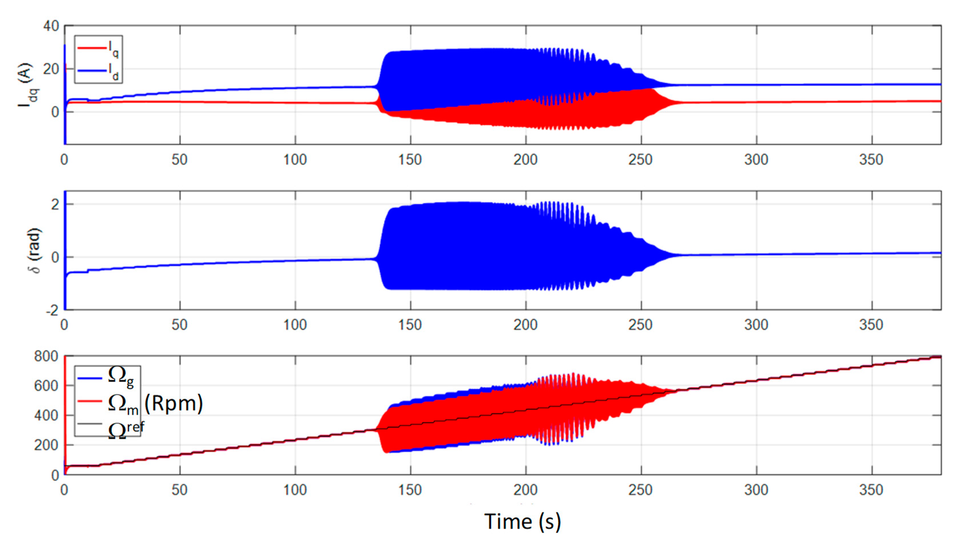
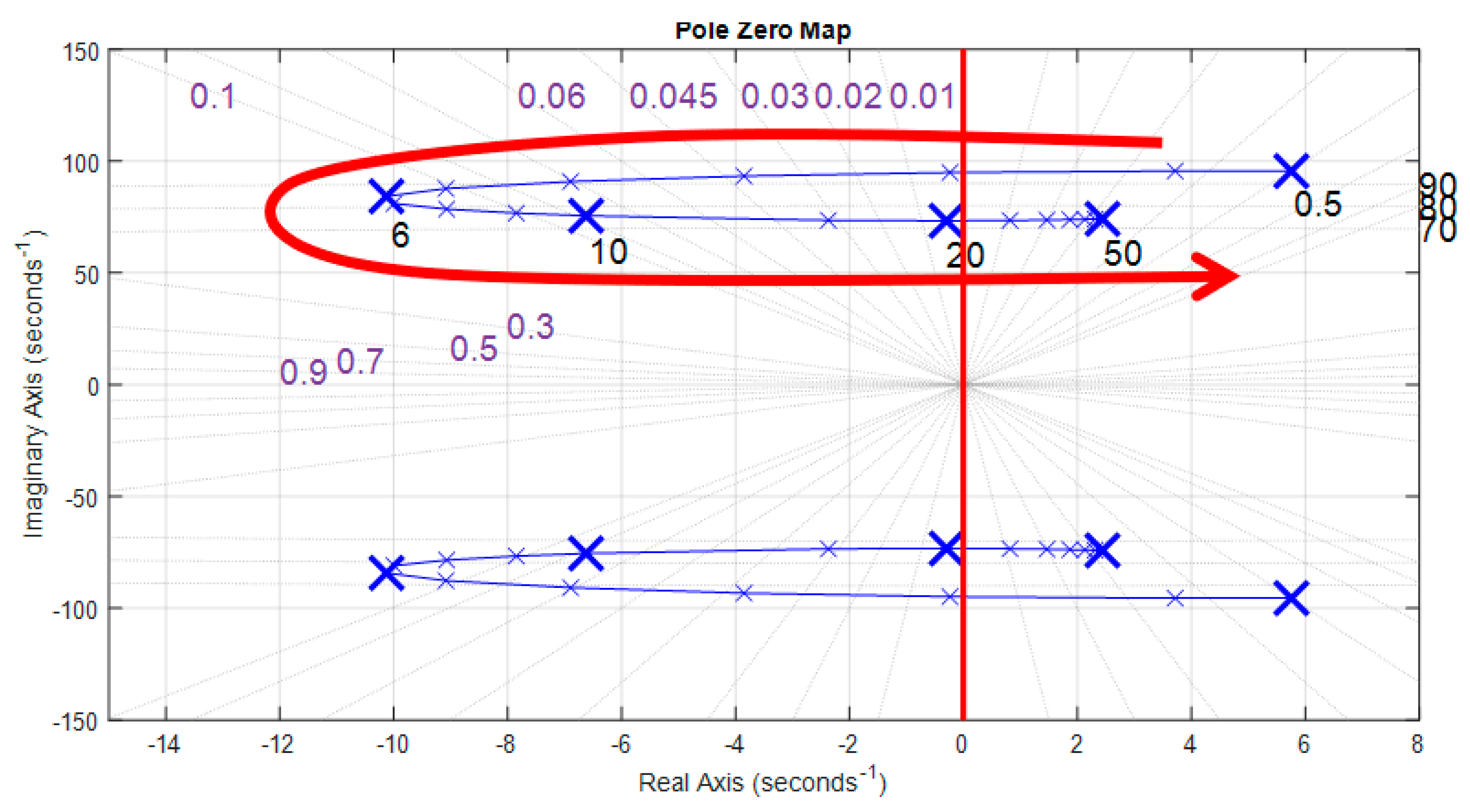
4.1. Stability Analysis with Respect to the Generator Speed

The first analysis relates to the original parametric configuration of the system in accordance with the experimental bench. Here the dynamic (bandwidth) of the speed control for the gas turbine—generator association is set to 1 Hz for the IP controller bandwidth with a damping coefficient equal to 1. On the propeller side, a linear torque-speed characteristic is applied: $T_{pro{p}_m}$=k.Ω; with k = 0.1 This choice is made for this preliminary study in order to avoid a nonlinearity at the input of the system, which could bring a possible additional complexity to the understanding of the instability phenomenon. This choice is possible as the evaluated speed range is quite low thus making it possible to approximate the propeller load with an equivalent linear load without making too much of an error.

This analysis is set with respect to an evolution of the generator speed.

Based on the linearized state model, the root locus is analytically derived with operating speed which varies step by step (every 10 rpm) between various steady-state points, here between 200 and 800 rpm for the generator mechanical speed. On that root locus, blue crosses denote the generator speed steady states while purple values are related to the system damping and black values on the right are related to the system angular frequency. Only the dominant poles close to the imaginary axis are represented here.

On the transient time simulation (Matlab Simulink) and on the experimental test rig, the protocol follows a similar approach as the system evolves between different stages of generator speed, ranging from 0 to 800 rpm. These stages are spaced 10 rpm apart, and are maintained for 5 s.

The root locus of Figure 7 shows that, inside a speed range between 260 and 620 rpm for the generator mechanical speed, the real parts of the poles are positive, indicating the unstable domain of the system.

The time simulation result of Figure 8 also highlights a phenomenon of instability similar to the one observed from the root locus analysis. It is indeed possible to find a generator speed range during which the AC powertrain becomes oscillating (phase of “quasi-instability”), these non-divergent oscillations being maintained in steady state. On the contrary, before and after this speed range, the behavior of the system remains perfectly stable. Moreover, the speed range of “quasi-instability” is emphasized by the simulation tool between 290 and 580 rpm, which is quite consistent with the unstable range obtained with the root locus (between 260 and 620 rpm).

This last comparison shows the concordance of the root locus analysis based on the analytic linearized state model and of the time simulation of the whole system, without any linearization.

The experimental results of the Figure 9 also underline the same phenomenon of “quasi-instability”. The experimental test bench has an oscillating speed range between 300 and 560 rpm, while its behavior is stable outside this interval. This speed range is also close to the previous ranges given by the theoretical means of study. It is then possible to conclude that the various means of study of the AC electric propulsion architecture match by indicating a domain of “quasi-instability”: consequently, this comparative analysis reveals a “heavy trend” that sets the system stability on a generator intermediate speed range at risk.

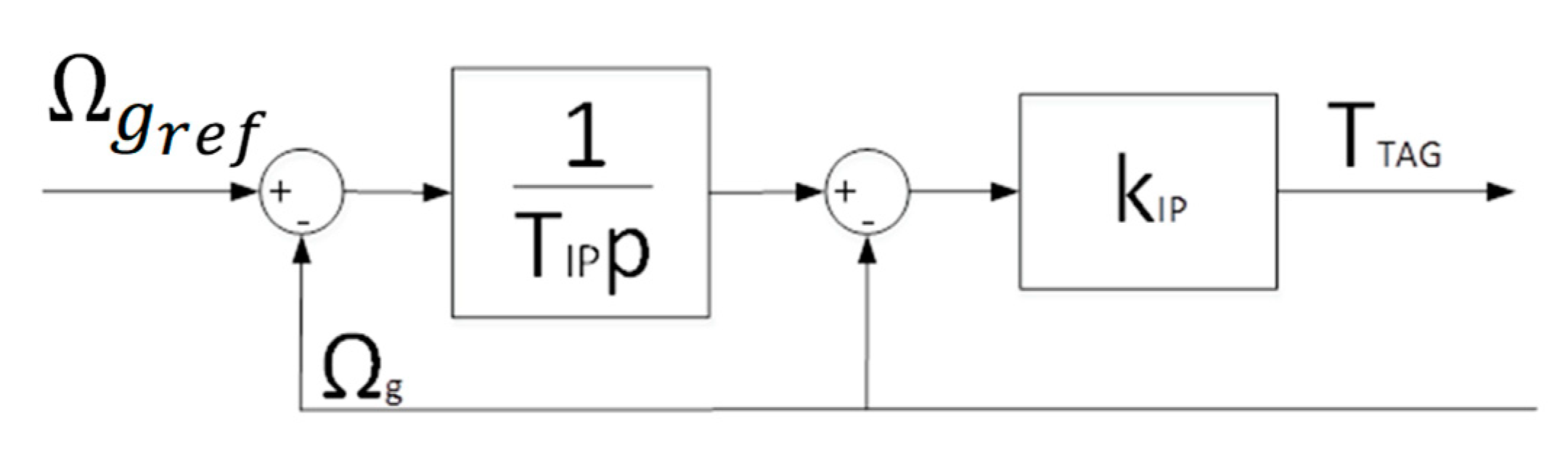
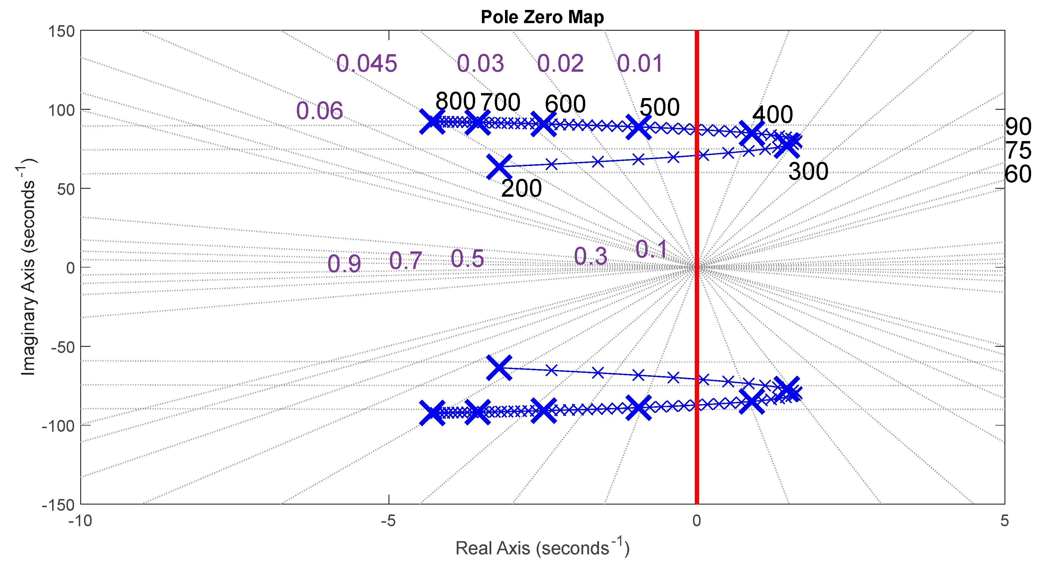
4.2. Influence of the Gas Turbine Control Dynamic on the Stability of the Powertrain

After having considered the stability analysis with respect to the generator, the issue is to analyze the influence of the gas turbine speed control dynamic on the system stability.

The gas turbine speed control dynamic, originally with a bandwidth set to 1 Hz, varies here between the following values (indicated in Hz): {0.9; 1; 1.25; 1.5; 1.75; 2}.

As in the previous analysis, the following figures show the results of the different means of study depending on the generator speed range but for a bandwidth of 0.9 Hz: Figure 10 presents the new root locus; time domain simulation is shown on Figure 11 and experimental performances on Figure 12.

For the other control dynamics, the results are summarized in

Table 2. Results of the different means of study for different gas turbine control dynamics.

Gas Turbine Dynamic (Hz)	Unstable Speed Range (rpm) from Root Locus	Unstable Speed Range (rpm) from Time Simulation	Unstable Speed Range (rpm) from Experiments
0.9	260 → 660 (Δ = 400)	280 → 610	270 → 620
1	260 → 620 (Δ = 360)	290 → 580	300 → 560
1.25	270 → 540 (Δ = 270)	310 → 510	310 → 530
1.5	280 → 480 (Δ = 200)	340 → 440	320 → 520
1.75	310 → 420 (Δ = 110)	No oscillation	320 → 380
2	No oscillation	No oscillation	No oscillation

. In that table, the speed range (Δ) with unstable behavior is displayed for the left column (related to the root locus analysis).

These different results firstly confirm the correct concordance between the different means of study of the AC electric propulsion architecture, except for the case of a bandwidth equal to 1.75 Hz, for which slight differences appear between the analysis tools. Indeed, for such a control dynamic, the system is “quasi stable” with slight oscillations appearing in experiments and being also predicted from the root locus. Contrarily these oscillations are not visible in the time simulation for this control dynamic. This can be explained by the fact that the unstable poles are very close to the ordinate axis, which characterizes the limit of stability.

These results also reveal a huge trend related to the tuning of the gas turbine control dynamic: “the higher the speed control dynamic the more stable the powertrain”.

However, this conclusion should be considered carefully, being only valid for low values of the control bandwidth. Indeed, this trend is reversed at high frequency of the control bandwidth, as it can be seen in Figure 13.

For a low gas turbine dynamic value, increasing its value tends to bring the mechanical poles back into the stable domain of the pole location and thus stabilize the system, as seen with the previous results. However, this is no longer the case at the highest bandwidth value, where an increase in the bandwidth value brings the mechanical poles back into the unstable domain of the pole location. Thus, a notion of optimal bandwidth value emerges, allowing to consider a setting offering the greatest possible stability to the AC electric propulsion architecture.

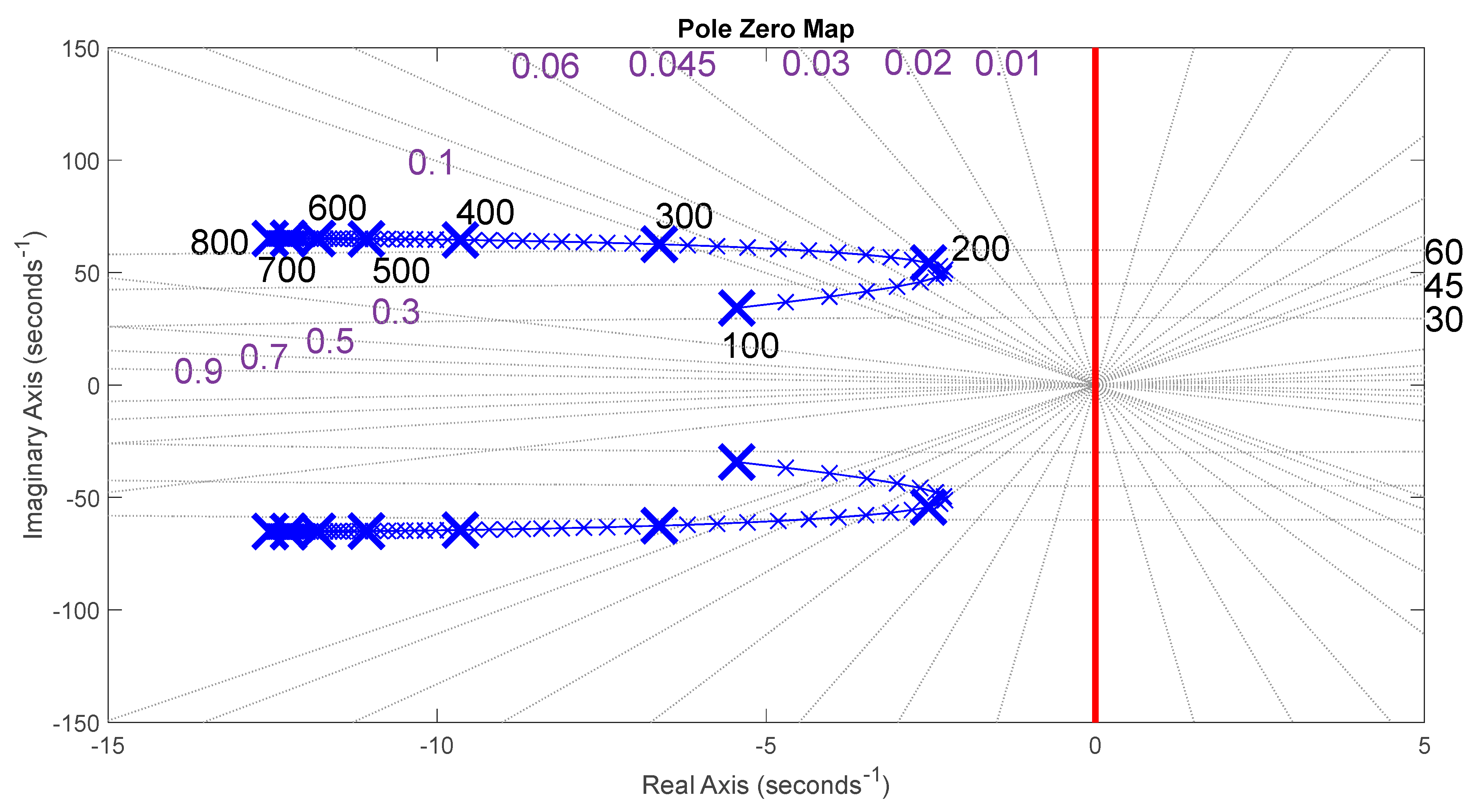
4.3. Influence of the Machine Inductances on the Stability of the Powertrain

The objective is now to consider the stability analysis with respect to certain key system parameters starting here with the machine inductances. In that case, the control dynamic is kept to a bandwidth of 1 Hz.

The initial values of the inductances of both machines connected through the AC bus are set to 6.5 mH for the generator and to 2.7 mH for the motor making a series inductance of 9.2 mH. The issue is here to increase this series inductance with added values between 1 and 6 mH.

The results of these parameter variations are summarized in

Table 3. Results of the different means of study for different series inductances values.

Addition of Inductances (mH)	Unstable Speed Range (rpm) from Root Locus	Unstable Speed Range (rpm) from Time Simulation	Unstable Speed Range (rpm) from Experiments
0 (base setting)	260 → 620 (Δ = 360)	290 → 580	300 → 560
1	240 → 560 (Δ = 320)	270 → 530	270 → 530
2	230 → 520 (Δ = 290)	250 → 490	250 → 500
3	210 → 480 (Δ = 270)	240 → 450	270 → 490
4	200 → 440 (Δ = 240)	230 → 420	250 → 470
5	190 → 420 (Δ = 230)	220 → 390	240 → 450

.

For all values of inductances, the results shown in Table 3 are consistent, although it should be noted that the reduction in the unstable speed range is less marked for the experimental results compared to the other two study methods. This slight difference can be explained: on the experiment, the physical addition of inductances may show slight unbalance between phases due to the use of single-phase inductances with potential differences, that may alter the observed phenomena. Contrarily, the added values of inductances are perfectly accurate for theoretical studies.

Nevertheless, whatever the means of study, it can be observed that increasing the series inductances of the AC bus coupling leads to:

-

Moving the unstable (oscillation) domain towards lower speeds;

-

A decrease in the speed range (Δ) inside which the AC powertrain is unstable or oscillates (on the left column, the unstable speed interval (Δ) is reduced by more than 30%.

In the same way, the influence of the load torque applied to the propeller on the system stability may complete that analysis. The results are not detailed in the paper, but the main trend shows that increasing the load level leads to an increase in the stability level of the powertrain.

4.4. Coupled Influence of System Parameters on the Stability of the Powertrain

The previous results have shown different influencing factors on the stability issue which were separately analyzed. This last subsection proposes a sensitivity analysis consisting of the observation of coupled effects due to various parametric variations on:

-

Inductances;

-

Magnetic flux of the magnets;

-

Inertia of the generator set (gas turbine—permanent magnet synchronous generator);

-

Inertia of the motor set (propeller—permanent magnet synchronous motor).

The original parameters of the system being displayed in Table 1, different parameter variations are proposed in

Table 4. Multi-parameter variations and associated results on the stability.

Parameters Modification	Unstable Speed Range (rpm) from Root Locus
No modification—Base setting	260 → 620 (Δ = 360)
10% increase in the generator and the motor inductances	240 → 570 (Δ = 330)↘
10% decrease in the generator and the motor inductances	280 → 680 (Δ = 400)↗
10% increase in the generator and the motor magnetic flux of the magnets	270 → 690 (Δ = 420)↗
10% decrease in the generator and the motor magnetic flux of the magnets	250 → 540 (Δ = 290)↘↘
10% increase in the inertia of the generator set	260 → 620 (Δ = 360)
10% decrease in the inertia of the generator set	260 → 610 (Δ = 350)↘
10% increase in the inertia of the motor set	260 → 580(Δ = 320)↘
10% decrease in the inertia of the motor set	260 → 660 (Δ = 400)↗

, in which only the unstable speed range based on the root locus analysis is displayed:

These results indicate various trends related to the speed range during which the system operation is seen as unstable. The rising, resp. falling, arrows are showing the variation (increasing, resp. decreasing) of the unstable speed range with respect to the performances obtained with the base settings (first row). It is possible to summarize the sizing trends which may improve the stability of the AC electric propulsion architecture:

-

Important inductances values;

-

Low electromotive forces (image of the magnetic fluxes);

-

Important inertia of the motor set.

-

In order to analyze the coupling effects between parameters and to verify potential antagonistic couplings, the following variations are simultaneously applied to the system:

-

10% increase in the generator and the motor inductances;

-

10% decrease in the generator and the motor magnetic flux of the magnets;

-

10% decrease in the inertia of the generator set;

-

10% increase in the inertia of the motor set.

The theoretical analysis under these coupled modifications is displayed on the Figure 14 for the root locus and Figure 15 for the time simulation:

Compared with the results of Figure 7 and Figure 8 related to the base parametric configuration, the stability level is clearly increased with narrow unstable speed range. Indeed, the unstable speed range (seen from the root locus) which was initially between 260 and 620 rpm (Δ =360 rpm) for the base parametric configuration is now between 240 and 450 rpm (Δ =210 rpm), showing a great improvement of the stability level of the powertrain.

It is even possible to find parametric configurations allowing a “full stable operation” of the AC electric propulsion architecture by imposing higher modifications following the same trends as above. For example, the following parametric configuration can be considered:

-

100% increase in the generator and the motor inductances;

-

25% decrease in the generator and the motor magnetic flux;

-

50% decrease in the inertia of the generator set;

-

25% increase in the inertia of the motor set.

The results of the theoretical means of study under the previous coupled modifications are displayed on the Figure 16 and Figure 17:

It is thus possible to conclude that following the identified design trends would make it possible to obtain an AC electric propulsion architecture with a full stable operation.

5. Conclusions

This paper relates to a typical electric powertrain for aircraft propulsion which is composed exclusively of permanent magnet synchronous machines (PMSM) without any power electronics. In particular, each PM synchronous generator is directly connected through an AC bus with a single or multi PM synchronous motor distribution set that drives the propelling system. Suppressing power electronics offers substantial gains in terms of embedded weight: some figures are proposed as example of weight reduction in the introductive section. However, suppressing power electronics and considering a direct (“rigid”) AC coupling of two or several PMSMs involves stability issues that are the main focus of the paper.

Before analyzing the system stability, several models and tools are built: a nonlinear transient state model of the AC electric propulsion architecture is firstly developed. In the framework of a time simulation, this model is compared with a circuit time simulation on the Saber solver showing the accordance between both tools.

Based on that nonlinear state model, a small-signal linearization is analytically derived, leading to the root locus definition of the AC powertrain that characterizes stable and unstable domains. This analytical approach allows achieving a sensitivity analysis linking system parameters with stability conditions.

This set of linear and nonlinear analysis tools is compared with a reduced power scale experimentation emulating the power architecture. Regarding the dynamic behavior and the system stability, all analysis means of study are quite in accordance, emphasizing the existence of unstable subdomains which depend on the physical and control parameters of the powertrain.

The sensitivity analysis shows that full stable operation may be obtained with specific system sizing and control tuning.

Let us note that the PMSMs studied in this paper correspond to small power machines for industry applications: these machines were the ones installed in the experimental reduced power scale test bench which has allowed us to validate the state models for stability analysis. It is clear that such machines differ from “specific machines” for aircraft propulsion. In our current studies, we are analyzing “scale one” electric machines more representative of the aircraft application. Preliminary results not presented in the paper show that major trends in terms of stability are mainly reproduced with these machines.

Furthermore, the trends shown are not necessarily compatible with a design that can be integrated into an aircraft that must ensure a robust and full stable system operation. On the other hand, the tools developed in this paper allow us to consider corrective solutions to the instability problem which constitutes the main prospect of this study.

References

1. Roland Berger, Think: Act, Navigating Complexity. Aircraft electrical Propulsion—Onwards and Upwards. 2018. Available online: https://www.rolandberger.com/publications/publication_pdf/roland_berger_aircraft_electrical_propulsion_2.pdf (accessed on 1 September 2022).
2. IATA. Aircraft Technology Roadmap to 2050. 2019. Available online: https://www.iata.org/contentassets/8d19e716636a47c184e7221c77563c93/Technology-roadmap-2050.pdf (accessed on 1 September 2022).
3. Sarlioglu, B.; Morris, C.T. More Electric Aircraft: Review, Challenges, and Opportunities for Commercial Transport Aircraft. IEEE Trans. Transp. Electrif. 2015, 1, 54–64. [Google Scholar] [CrossRef]
4. Roland Berger. Electric Propulsion Is Finally on the Map. Available online: https://www.rolandberger.com/en/Insights/Publications/Electric-propulsion-is-finally-on-the-map.html (accessed on 1 September 2022).
5. Epstein, A.H.; O’Flarity, S.M. Considerations for Reducing Aviation’s CO2 with Aircraft Electric Propulsion. J. Propuls. Power 2019, 35, 572–582. [Google Scholar] [CrossRef]
6. Pornet, C.; Isikveren, A. Conceptual design of hybrid-electric transport aircraft. Prog. Aerosp. Sci. 2015, 79, 114–135. [Google Scholar] [CrossRef]
7. Ansell, P.J.; Haran, K.S. Electrified Airplanes: A Path to Zero-Emission Air Travel. IEEE Electrif. Mag. 2020, 8, 18–26. [Google Scholar] [CrossRef]
8. Madonna, V.; Giangrande, P.; Galea, M. Electrical Power Generation in Aircraft: Review, Challenges, and Opportunities. IEEE Trans. Transp. Electrif. 2018, 4, 646–659. [Google Scholar] [CrossRef]
9. Thauvin, J. Exploring the Design Space for a Hybrid-Electric Regional Aircraft with Multidisciplinary Design Optimisation Methods. Ph.D. Thesis, Institut National Polytechnique de Toulouse (Toulouse INP), Toulouse, France, 2018. Available online: https://oatao.univ-toulouse.fr/23607/1/Thauvin_jerome.pdf (accessed on 1 September 2022).
10. Clarke, S.; Redifer, M.; Papathakis, K.; Samuel, A.; Foster, T. X-57 power and command system design. In Proceedings of the 2017 IEEE Transportation Electrification Conference and Expo (ITEC), Chicago, IL, USA, 22–24 June 2017; pp. 393–400. [Google Scholar] [CrossRef] [Green Version]
11. Dillinger, E.; Döll, C.; Liaboeuf, R.; Toussaint, C.; Hermetz, J.; Verbeke, C.; Ridel, M. Handling qualities of ONERA’s small business concept plane with distributed electric propulsion. In Proceedings of the 31st Congress of International Council of Aeronautical Sciences (ICAS), Belo Horizonte, Brazil, 9–14 September 2018; pp. 1–10. [Google Scholar]
12. Bidart, D.; Pietrzak-David, M.; Maussion, P.; Fadel, M. Mono inverter multi-parallel permanent magnet synchronous motor: Structure and control strategy. IET Electr. Power Appl. J. 2011, 5, 288–294. [Google Scholar] [CrossRef] [Green Version]
13. Sahoo, S.; Zhao, X.; Kyprianidis, K. A Review of Concepts, Benefits, and Challenges for Future Electrical Propulsion-Based Aircraft. Aerospace 2020, 7, 44. [Google Scholar] [CrossRef] [Green Version]
14. Mouty, S. Conception de Machines à Aimants Permanents à Haute Densité de Couple Pour les éoliennes de Forte Puissance. Ph.D. Thesis, Université de Franche-Comté, Besancon, France, 2013. [Google Scholar]
15. Courtecuisse, V. Supervision d’une Centrale Multisources à Mase d’éoliennes et de Stockage d’énergie Connectée au Réseau électrique. Ph.D. Thesis, Ecole Nationale Supérieure d’Arts et Métiers, Paris, France, 2008. [Google Scholar]
16. Merwerth, J. The Hybrid-Synchronous Machine of the New BMW i3 & i8. 2014. Available online: https://www.speakev.com/attachments/20140404_bmw-pdf.80577/ (accessed on 1 September 2022).
17. Alstom. AGV-Le 21ème Siècle à Très Grande Vitesse. 2009. Available online: https://docplayer.fr/205073-Agv-le-21-eme-siecle-a-tres-grande-vitesse.html (accessed on 1 September 2022).
18. Pinheiro, M.D.L.; Suemitsu, W.I. Permanent magnet synchronous motor drive in vessels with electric propulsion system. In Proceedings of the 2013 Brazilian Power Electronics Conference, Gramado, Brazil, 27–31 October 2013. [Google Scholar] [CrossRef]
19. Bordianu, A.; Samoilescu, G. Electric and Hybrid Propulsion in the Naval Industry. In Proceedings of the 2019 11th International Symposium on Advanced Topics in Electrical Engineering (ATEE), Bucharest, Romania, 28–30 March 2019. [Google Scholar] [CrossRef]
20. Thongam, J.S.; Tarbouchi, M.; Okou, A.F.; Bouchard, D.; Beguenane, R. Trends in naval ship propulsion drive motor technology. In Proceedings of the 2013 IEEE Electrical Power & Energy Conference, Halifax, NS, Canada, 21–23 August 2013. [Google Scholar] [CrossRef]
21. Pettes-Duler, M. Integrated Optimal Design of a Hybrid-Electric Aircraft Powertrain. Ph.D. Thesis, Institut National Polytechnique de Toulouse (INPT), Toulouse, France, 2021. [Google Scholar]
22. Pettes-Duler, M.; Roboam, X.; Sareni, B. Integrated Optimal Design for Hybrid Electric Powertrain of Future Aircrafts. Energies 2022, 15, 6719. [Google Scholar] [CrossRef]
23. Blackwelder, M.J.; Rancuret, P.M. Multiple Generator Synchronous Electrical Power Distribution System. U.S. Patent EP3197043A1, 26 July 2017. [Google Scholar]
24. Armstrong, M.; Blackwelder, M. Combined AC and DC Turboelectric Distributed Propulsion System. U.S. Patent EP3318492A1, 9 May 2018. [Google Scholar]
25. Armstrong, M.; Blackwelder, M.J.; Bollman, A.M. Synchronizing Motors for an Electric Propulsion System. U.S. Patent US20160365810A1, 15 December 2016. [Google Scholar]
26. Bachmann, C.; Bergmann, D.; Bachmaier, G.; Gerlich, M.; Pais, G.; Vittorias, I. Propellerantrieb und Fahrzeug, Insbesondere Flugzeug. Germany Patent DE102015213580A1, 26 January 2017. [Google Scholar]
27. Himmelmann, R.A. Variable Speed AC Bus Powered Tail Cone Boundary Layer Ingestion Thruster. U.S. Patent US20180265206A1, 20 September 2018. [Google Scholar]
28. Rougier, F.; Viguier, C. Système Electrique Pour Canal Propulsif Synchrone. France Patent FR3092948A1, 21 August 2020. [Google Scholar]
29. Sadey, D.J.; Taylor, L.M.; Beach, R.F. Proposal and Development of a High voltage Variable Frequency alternating Current Power System for Hybrid Electric Aircraft. In Proceedings of the 14th International Energy Conversion Engineering Conference, Salt Lake City, UT, USA, 25–27 July 2016. [Google Scholar] [CrossRef] [Green Version]
30. Sadey, D.J.; Bodson, M.; Csank, J.T.; Hunker, K.R.; Theman, C.J.; Taylor, L.M. Control Demonstration of Multiple Doubly-Fed Induction Motors for Hybrid Electric Propulsion. In Proceedings of the 53rd AIAA/SAE/ASEE Joint Propulsion Conference, Atlanta, GA, USA, 10–12 July 2017. [Google Scholar] [CrossRef]
31. Kundur, P. Power System Stability and Control; Power System Engineering Series; Electric Power Research Institute: Palo Alto, CA, USA, 1993. [Google Scholar]
32. Saber Simulation Solver. Available online: https://www.synopsys.com/verification/virtual-prototyping/saber.html (accessed on 1 November 2022).
Figure 1. Several topologies for the powertrain: (a) with power electronics coupling; (b) single-motor “power electronic-less” coupling; (c) multi-motor “power electronic-less” coupling.
Applsci 13 00672 g001
Figure 2. Two example of architectures (here with six propellers) with direct AC coupling between generators and motors.
Applsci 13 00672 g002
Figure 3. Park’s reference frames: (a) generator voltage and current vectors in the generator reference frame (dg,qg); (b) motor voltage and current vectors in the motor reference frame (dm,qm); (c) generator and motor voltage and current vectors with phase shift in the generator reference frame (dg,qg).
Applsci 13 00672 g003
Figure 4. IP speed control of the gas turbine—generator association.
Applsci 13 00672 g004
Figure 5. Comparison of time simulations between the analytic state model simulated on Matlab Simulink (red curves) and the circuit simulation on Saber (blue curves).
Applsci 13 00672 g005
Figure 6. Reduced power scale test bench for AC powertrain functional emulation.
Applsci 13 00672 g006
Figure 7. Small-signal model-based root locus with respect to the generator speed (blue crosses) with a bandwidth of 1 Hz for the generator speed control. Dashed lines illustrate iso-values of system damping (linear dashed lines), and iso-values of system angular frequency (horizontal dashed lines), the red line indicate the limit between stable and unstable zone: the ordinates axe.
Applsci 13 00672 g007
Figure 8. Time simulation with respect to variable stages of the generator speed with a bandwidth of 1 Hz for the generator speed control.
Applsci 13 00672 g008
Figure 9. Experimental test with respect to variable stages of the generator speed with a bandwidth of 1 Hz for the generator speed control.
Applsci 13 00672 g009
Figure 10. Small-signal model-based root locus with respect to the generator speed (blue crosses) with a bandwidth of 0.9 Hz for the gas turbine speed control.
Applsci 13 00672 g010
Figure 11. Time simulation with respect to variable stages of the generator speed with a bandwidth of 0.9 Hz for the gas turbine speed control.
Applsci 13 00672 g011
Figure 12. Experimental test with respect to variable stages of the generator speed with a bandwidth of 0.9 Hz for the gas turbine speed control.
Applsci 13 00672 g012
Figure 13. Small-signal model-based root locus with respect to the gas turbine control dynamic (blue crosses) with a bandwidth varying between 0.5 and 50 Hz (with a constant speed of 400 rpm).
Applsci 13 00672 g013
Figure 14. Small-signal model-based root locus analysis for coupled parametric modifications with a bandwidth of 1 Hz for the generator speed control and with coupled modifications of electric and mechanical parameters.
Applsci 13 00672 g014
Figure 15. Time simulation analysis for coupled parametric modifications with a bandwidth of 1 Hz for the generator speed control and with coupled modifications of electric and mechanical parameters.
Applsci 13 00672 g015
Figure 16. Small-signal model-based root locus analysis for the previous coupled parametric modifications with a bandwidth of 1 Hz for the generator speed control and with coupled modifications of electric and mechanical parameters.
Applsci 13 00672 g016
Figure 17. Time simulation result of the stability analysis for the previous coupled parametric modification with a bandwidth of 1 Hz for the generator speed control and with coupled modifications of electric and mechanical parameters.
Applsci 13 00672 g017