

R Libraries for Remote Sensing Data Classification by K-Means Clustering and NDVI Computation in Congo River Basin, DRC


Laboratory of Image Synthesis and Analysis (LISA), École Polytechnique de Bruxelles (EPB, Brussels Faculty of Engineering), Université Libre de Bruxelles (ULB), Building L, Campus de Solbosch, ULB—LISA CP165/57, Avenue Franklin D. Roosevelt 50, B-1050 Brussels, Belgium
*
Author to whom correspondence should be addressed.
Appl. Sci. 2022, 12(24), 12554; https://doi.org/10.3390/app122412554
Submission received: 6 October 2022
/
Revised: 20 November 2022
/
Accepted: 30 November 2022
/
Published: 7 December 2022
(This article belongs to the Special Issue Geoinformatics and Remote Sensing Applications for the Current Needs for Environmental Management and Protection)
Abstract
:Featured Application
Libraries of the R programming language, including RStoolbox, raster and terra, were used to classify Landsat OLI-TIRS satellite images by k-means clustering and NDVI computation for comparative vegetation mapping of tropical rainforests for the period of 2013–2022 in the three target areas (Bumba, Basoko, Kisangani) of the middle Congo River Basin, central Africa, D.R.C.
Abstract
In this paper, an image analysis framework is formulated for Landsat-8 Operational Land Imager and Thermal Infrared Sensor (OLI/TIRS) scenes using the R programming language. The libraries of R are shown to be effective in remote sensing data processing tasks, such as classification using k-means clustering and computing the Normalized Difference Vegetation Index (NDVI). The data are processed using an integration of the RStoolbox, terra, raster, rgdal and auxiliary packages of R. The proposed approach to image processing using R is designed to exploit the parameters of image bands as cues to detect land cover types and vegetation parameters corresponding to the spectral reflectance of the objects represented on the Earth’s surface. Our method is effective at processing the time series of the images taken at various periods to monitor the landscape dynamics in the middle part of the Congo River basin, Democratic Republic of the Congo (DRC). Whereas previous approaches primarily used Geographic Information System (GIS) software, we proposed to explicitly use the scripting methods for satellite image analysis by applying the extended functionality of R. The application of scripts for geospatial data is an effective and robust method compared with the traditional approaches due to its high automation and machine-based graphical processing. The algorithms of the R libraries are adjusted to spatial operations, such as projections and transformations, object topology, classification and map algebra. The data include Landsat-8 OLI-TIRS covering the three regions along the Congo river, Bumba, Basoko and Kisangani, for the years 2013, 2015 and 2022. We also validate the performance of graphical data handling for cartographic visualization using R libraries for visualising changes in land cover types by k-means clustering and calculation of the NDVI for vegetation analysis.
Keywords:
image processing; remote sensing; Landsat; R language; programming; cartography; mapping; data visualization; NDVI; AfricaPACS:
91.10.Da; 91.10.Jf; 91.10.Sp; 91.10.Xa; 96.25.Vt; 91.10.Fc; 95.40.+s; 95.75.Qr; 95.75.Rs; 42.68.WtMSC:
86A30; 86-08; 86A99; 86A04JEL Classification:
Y91; Q20; Q24; Q23; Q3; Q01; R11; O44; O13; Q5; Q51; Q55; N57; C6; C611. Introduction
Satellite image processing is a fundamental problem in remote sensing data analysis and is a key step towards the automatic visualization of the Earth’s landscapes. The significance of the satellite images for visualising the Earth is that they incorporate rich information about the land cover types, which can be derived from the interpretation of the pixels. The brightness of pixels in the satellite images correspond to the spectral reflectance of various surfaces and objects: built-up urban areas, bare soil, deserts, forest and various vegetation types, water areas, etc. Since the absorption of solar radiation varies in these objects, their spectral reflection is different. Such fundamental properties of optics of the materials form a basis for the environmental applications of satellite imagery generated by the sensors onboard the satellites [1]. The differences in spectral signatures of the surfaces are detectable in bands, or channels, of the satellite imagery and digital numbers (DNs) of the pixels in bitmap images, which can be used for land cover mapping [2].
Satellite images processed by remote sensing tools are often used to visualise landscape dynamics as a way to detect land cover changes by exploiting the similarities and differences in pixels of the images from Landsat [3,4] or Sentinel [5,6,7] or their integration [8,9]. Some of the methods of image processing use time series analysis using fine spatial resolution imagery [10,11], topological data extraction by spectral analysis derived from Synthetic Aperture Radar (SAR) [12,13], photogrammetry or Light Detection and Ranging (LiDAR) processing to analyse forest canopy by collecting 3D data [14]. Additionally, image processing may use a supervised classification approach, which includes automated extraction of the training samples and reference maps [15], regression tree analysis for canopy height modelling [16], or statistical methods to analyse forest degradation [17].
The spectral bands that comprise the satellite imagery consist of a matrix of pixels. Different intensities of the wavelengths of light of the pixels are visible on the image as colours of various hues and shadowing. The Landsat OLI/TIRS consists of 11 bands, including spectral bands: ultra violet (UV), visual, near-infrared (NIR), short-wave infrared (SWIR) and thermal infrared (TIR). Red and NIR bands, which correspond to channels 4 and 5, are specifically useful for vegetation analysis and forest mapping, as has been demonstrated in related works [18,19,20]. This is explained by the chlorophyll reflectance of plants in the red/NIR zones, which can be used as an arithmetic combination of bands 4–5 for computing the Normalized Difference Vegetation Index (NDVI) [21] or other vegetation indices [22,23] as indicators of vegetation health, vigour, and plant phenology, as reported earlier [24,25,26,27].
The modelling, reconstruction and prognosis of tropical forest degradation in Africa poses a challenge for both environmental research as well as socio-economic applications, since deforestation affects the current land use policies and agro-industrial development of central African countries [28,29]. In addition to climate factors, selected human activities, such as timber production, road expansion, logging and manufacturing, contribute to deforestation [30,31,32]. Another factor includes the high consumption of wood by local population through agriculture and woodcutting [33]. At the same time, deforestation and the unbalanced functioning of forest ecosystems have wider effects and environmental consequences including land degradation, desertification, the loss of wildlife habitat and soil erosion [34]. Analysis of deforestation is possible by comparing forest areas on older maps with those detected on the remote sensing data [35,36,37] or landscape dynamics evaluated by time series of images [38]. Other approaches include continuous metrics to measure the degree of forest degradation [39]
While the techniques of the remote sensing data acquisition and image processing by Geographic Information System (GIS) have demonstrated advances over recent decades [40,41], the algorithms of geospatial data modelling are not as straightforward regarding handling the data automatically. At the same time, the required automation is possible using the programming approaches. A large number of methods focused on forest monitoring by the remotely sensed data have been proposed over recent years [42,43,44,45,46]. Popular cases include the use of multi-source data, such as a fusion of LiDAR, radar and optical data, very high-resolution satellite images and unmanned aerial vehicles (UAV) [47], as well as the application of Land Use/Land Cover (LULC) change [48], classification and clustering [49], and integration of the remote sensing data with reference maps for change detection [50]. Typically, methods of forest mapping are based on the use of Landsat imagery [51,52,53], though others utilize SAR [54,55,56,57,58] or Moderate Resolution Imaging Spectroradiometer (MODIS) scenes [59,60] for land cover classification in forest areas.
Compared with GIS, the use of programming languages for image processing presents new possibilities in mapping through the extended functionality of algorithms and has received much attention in the geoscience community [61,62,63,64,65]. As previous work shows [66,67,68], integrating spatial information from the satellite images using various perceptual tasks, such as object recognition, location, classification and interpretation, are necessary for disambiguating visually similar land cover classes of the Earth’s surface representing the landscapes. The automatic recognition of the diverse land cover classes on various periods facilitates the recognition of the environmental changes. However, misclassifications remain in challenging situations with similar classes with human-based interpretation using supervised classification GIS for image analysis [69,70,71]. This requires us to recognise and classify all possible occurrences of pixels in the scenes automatically, which is a computationally effective task using programming algorithms.
In this paper, we propose an application of R programming language [72] as a means to process and classify satellite images. Specifically, we presented the unsupervised classification of the Landsat-8 OLI/TIRS data and calculation of the Normalized Difference Vegetation Index (NDVI) based on RSToolbox, raster and terra packages. Motivated by recent reports regarding the environmental changes in rainfall tropical forests of central Africa [10,73,74,75,76,77], we applied multi-temporal data covering identical selected regions along the middle Congo River Basin with a time span of 2013 to 2022. The practical aim is to demonstrate the dynamics of the landscapes within a decade using Landsat satellite images. Our methods apply k-means automated clustering and calculate the NDVI index using the R libraries RStoolbox [78], terra [79], and raster [80] and auxiliary graphical packages such as RColorBrewer [81] and viridis [82].
2. Study Area
The dataset contains satellite images obtained for the region of the Democratic Republic of Congo (DRC) with the three target areas located in the middle region of the Congo River Basin, according to the regional division [83]. The surroundings of the towns Bumba, Basoko and Kisangani are located on the Congo River, which serves as the main transportation artery in the region (Figure 1).
Kisangani is the capital of the Tshopo province, situated at the confluence of the rivers Congo, Lualaba, Tshopo, and Lindi. It is strategically located at the crossroads between the eastern and western parts of Congo. Basoko town is situated in the confluence of the Aruwimi tributary into the Congo River. Bumba is a small town and a river port in the Mongala Province, which is in the northern part of the DRC. As a part of the Congo River Basin, these cities have a tropical monsoon climate with a dry winter period and humid summer-autumn seasons with heavy precipitation and periodically flooded areas [84]. Such a climate setting, characterised by rainfalls interspersed with a dry season climate, in the Congo Basin creates favourable conditions for the distribution of the world’s largest tropical humid forests [85].
The importance of the study area is explained by the crucial environmental role of the Congo River Basin. It contains over half of the African tropical moist forests, with Salonga National Park being the largest rain forest park in the world [86], and it largely contributes to the Earth’s atmosphere’s circulation on the planetary scale. Furthermore, the tropical rainforests of Congo are a key factor in producing oxygen and regulating global temperature through the absorption of solar radiation by forest massifs. Moreover, forest resources offer critical and principal support to the welfare of rural livelihoods and the socioeconomic wellbeing of the local population [87], which includes forest-related practices such as forest clearing. As a result, land use and shifting agriculture have become the major causes of the hydrological flow regime, environmental changes from the regional to global scale [88], as well as deforestation, along with the increased population density and associated urban growth [89].
At the same time, primary forests are essential ecosystems that play a key role in mitigating climate change, which raises the need to take action by mitigating the effects from deforestation and resilient development in forest degradation [90,91]. Efforts to conserve natural resources in Congo tropical rainforests recently launched global initiatives, such as Reducing Emissions from Deforestation and Forest Degradation (REDD+) [92,93] and the Global Rain Forest Mapping (GRFM) project [94]. On a regional and local level, practicing agroforests serve as ecosystem services responding to the climate change mitigation strategy [95]. Nevertheless, the Congo River Basin remains the least studied region in Africa and in the global tropics [96]. The approach we present here contributes to the development of methods for the environmental analysis of the selected regions of the Congo River Basin using remote sensing data and R programming.
3. Materials and Methods
This article proposes a general, fully automated method for classifying satellite images using R libraries by machine-based k-means clustering, which requires no prior information and no learning on land cover classes. On one hand, the nature of land cover types is captured by considering the spectral attributes of the pixels in the respective Landsat bands. By carefully analysing these attributes, we reveal and demonstrate that the irregularity of the spectrum in the wavelength corresponding to the landscape properties is highly related to the reflectance of the surface, which results in the brightness of pixels in the image. Thus, we applied the computational model of R to effectively capture and visualise this irregularity and transfer it from the frequency optical domain to the geo-information domain.
3.1. Research Design
Within the scope of the current study, the functionality of R is focused on the K-means clustering classification algorithm of RStoolbox to process the satellite images, with the aim of visualising and comparing the extent of vegetation in the central Congo River Basin for different years using a general workflow approach, as seen in Figure 2. The Landsat satellite images taken in 2013, 2015 and 2022 were used to visualise change detection between land cover or forest types. Thus, the algorithms of R support the operational monitoring of the dynamics of land cover types derived from the images. However, the packages of R can also be applied to additional applications of geospatial data analysis where automated image classification is needed. Examples of such cases include monitoring the desertification using time series of images, analysis of urban growth using retrospective data overlaid with current maps and actual images, or forest fire monitoring.
The functionality of R programming presents a set of modular functions for the automation of image classification applications from Earth observation, spatial and remote sensing data, as seen in Figure 3.
The packages of ‘terra’ and ‘raster’ include the functionality of pre- and post-processing of both data types (vector and raster), as well as extensible features for spatial data analysis. Raster data analysis includes reading the information on the spectral reflectance of the image bands, automated processing of the stacked bands, feature extraction for unsupervised classification using clustering, creating multi-layer colour composites, performing map algebra using raster bands, visualising the thematic maps as overlays, classification and basic statistical analysis, such as histograms.
R operates with major features of spatial data, such as dimensions, resolution, reading data extent (min/max analysis), plotting the data, manipulating with Coordinate Reference Systems (CRS), reprojecting the data, assigning the CRS and transforming the data. An important function of R ‘terra’ package consists of creating the SpatRaster objects, which are a class of raster data with a longitude/latitude CRS as spatial parameters and a specific geometry of the file (cells are arranged in the rows/columns of the internal grid). Moreover, the ‘terra’ package enables the cartographic visualization of continuous fields, including topographic elevation, vegetation based on the classified land cover types, and climate data in a spatial context (regional variations in temperature and precipitation). Furthermore, R enables us to perform data clipping using an overlay of spatial data and imagery over their area of interest.
3.2. Data
The first step in the workflow included downloading data from the USGS GloVis data repository, which offers a global coverage of the publicly available satellite images with open access. We selected the three areas of Bumba, Basoko and Kisangani and collected the Landsat-8 OLI/TIRS imagery for the dates 2013 and 2022. The exact Landsat Product IDs are summarised in Table 1. The main characteristics of the imagery are summarised in Table 2.
The common technical parameters for all the scenes are as follows: spacecraft ID—Landsat 8; origin: USGS; station ID—LGN; sensor ID—OLI_TIRS; processing level—L1TP; collection number—2; collection category—T1; output format—GEOTIFF; WRS type—2; datum and ellipsoid—WGS84; data source elevation—GLS2000; GCP version—5.
The used images are categorised by the L1TP Level 1 Precision Terrain (corrected), which are the DNs in a 16-bit integer format, converted to the top-of-atmosphere (TOA) spectral reflectance (Bands 1–9) or radiance (Bands 1–11) using scaling factors [97]. The L1TP images include radiometric, geometric, and precision correction and use a digital elevation model (DEM) to correct errors caused by the local topographic relief; the accuracy of the precision/terrain-corrected product depends on the ground control points (GCPs) obtained from the GLS2000 dataset and the resolution of the DEM. Thus, the geometric accuracy of the L1TP Landsat images is valiadated using the ground control points (GCP), which are derived from the GLS2000 library. These data are used for computing the RMSE of the geometric residuals on the terrain-corrected images [97].
An additional image for 2015 was selected for Kisangani due to the higher cloud coverage in 2013. The geographic map in Figure 1 has been plotted using the generic mapping tools (GMT) defined by scripts following the existing methodology [98,99,100]. The study area encompasses the middle Congo river basin with the three specific towns of Bumba, Basoko, and Ksangani, located in consecutive order southwards. The collected data were inspected for metadata using R Listing 1.
| Listing 1: R code used for data inspection by rGDAL and raster libraries; here a case of Basoko town applied for all other images. |
  |
We explored the ‘rgdal’ library of R to retrieve the coordinates and check the topology and spatial dimensions of the dataset stored in the SpatialGridDataFrame class. AThetopology refers to the arrangement of the images that defines the coincident geometry of the feature classes from the Landsat dataset. It reads the contextual information from the structure data based on spatial relationships, specifically the adjacency of the coordinates and connectivity of overlapping images. The RasterLayers were generated as the arrays of pixels from the individual bands of the Landsat scenes. Afterwards, a facetted stack was created using the Landsat OLI-TIRS bands via the stack() function. To this end, the ‘raster’ R library was applied to concatenate the multiple bands into a single bitmap image, which used the data on the origin of the coordinates of each band. The resulting image was visualized by the plot() function of R. The number of layers of and spatial dimension in the new multi-layer object of R were inspected by the ’raster’ library. The resolution of all the layers was 30 m, except for the panchromatic band (15 m) and the two last TIRS layers, with a coarser resolution of 100 m. The selected band was plotted in a grayscale monochrome visualization. The data analysis and inspection was performed using Listing 1.
3.3. Plotting Band Composites
We explored the structure of the Landsat bands by inspecting the metadata. The image of all the bands is visualized as a representation of the monochrome multi-facetted plot in Figure 4. The majority of the multispectral bands have 30 m resolution, while the panchromatic band (B8) has a higher resolution (15 m), and the two TIRS (B10 and B11) have a coarse 100 m resolution. Generating colour composites by a combination of various band triplets provides more information, which can be effectively exploited using the ‘raster’ and ’terra’ libraries of R. Here the idea of the machine-assisted classifier by R packages consists of the identification of the spectral reflectance of the pixels constituting the 11 bands for thematic mapping.
The sensor instruments of Landsat-8 OLI-TIRS record more channels of data than are actually needed for vegetation applications. For instance, to calculate the NDVI, we only need the Red and NIR bands (4 and 5, respectively). However, combining the bands in various RGB triplets enables us to highlight diverse objects on the surface to discriminate and capture information on a wider variety of objects. Thus, the composition of red, green and blue colours creates images with varied hue, saturation and intensity representations owing to the pixel brightness as the spectral reflectance of the objects and surfaces on the Earth. Therefore, the bands were mixed to form various colour composites and inspect the land cover types. The selected and most representative band composites for the three main studied regions were plotted as natural and false colour composites, respectively, which were generated using the ’raster’ library. A relevant code snippet is given for the town of Basoko and was applied similarly for the rest of the Landsat-8 OLI-TIRS scenes with changed parameters, as per Listing 2.
The multi-facetted plot of the individual bands of the Landsat OLI/TIRS image has been plotted using libraries ‘raster’ and ‘terra’ (version 1.2.11), by the code in Listing 3. Here the case is given for the image covering Basoko (2022), applied for other scenes.
| Listing 2: R code used for colour composites by libraries raster and terra; here a case of Bumba town applied likewise for all the other images. |
 |
| Listing 3: R code used for the monochrome individual bands of the image Landsat OLI/TIRS. |
 |
The generated images reveal spatial details that can be better discerned in the intensity of pixels in false colour composites for water areas and more sharpened representations of urban areas in the natural colour composites showing spatial details in the three target areas: Bumba, Basoko and Kisangani (Figure 5). The colour products for all the three regions were prepared using the combination of bands 4-3-2 (natural) and 5-4-3 (false) with spatial resolution selected as three triplets of the original multispectral bands of the Landsat-8 OLI/TIRS. The new mixture of the RGB bands was converted to the colours with the intensity channel corresponding to the resolution of the original bands (30 m). Hue, saturation and intensity transformations of each of the triplets were resampled by R package ’terra’ to form the output image, Figure 5.
The above-demonstrated scripts show the key advantage of R, which consists of the optimization of the workflow of remote sensing data processing. Moreover, it illustrates its advanced analysis capabilities aimed at processing raster data by scripting. Scripts can be re-used with modified lines of code for the next images as a consecutive work, rather than repeated as a whole process of image analysis for each image, as in GIS, which is a fundamentally different approach compared to GIS. This is especially true for processing big Earth observation data, which play a key role in geoscience. The rapid development of remote sensing technologies has resulted in an increased amount of available satellite images, which requires advanced technologies for processing these large massifs of spatial data. In contrast to the traditional software, programming languages provide an effective solution to handle such volumes of spatial data by scripting. R, as an example of a high-level programming language, effectively solves the problem of the optimization of image processing.
3.4. K-Means Clustering
The k-means clustering of the R package RasterStack is a method by which pixels are assigned to spectral classes by machine-based partitions without prior knowledge of those classes. It is a straightforward way to produce a map of land cover classes using an automatic approach to image classification. The algorithm has been executed using an image-partitioning algorithm that infers the labels of the land cover classes by analysing intra-class similarity and, vice versa, the contrast between the classes. This method presents a machine learning approach for assigning pixels into the defined groups (or coherent clusters) according to their intensity and brightness, as seen in Listing 4. The clustering and classification of data is a commonly accepted practice for land cover mapping aimed at modelling changes in a forest structure by examining land-use categories [2,54,88,101,102].
| Listing 4: R code used for running the unsupervised classification by k-means clustering; here a case of Basoko town applied for all other images. |
  |
The image for classification was generated by stacking the data, which enabled us to create the RasterStack as a collection of RasterLayer objects. In turn, they were generated from the raster layers of the selected bands with the same spatial extent and resolution, that is, 30 m for the most of the Landsat-8 OLI/TIRS bands. Afterwards, RasterStack was merged into a RasterBrick, which is a multi-layer raster object created from the multi-layer files of RasterStack, made up of Landsat bands. The similarity between the RasterStack and RasterBrick classes consists in the fact that both are generated with a stack of the raster Landsat bands. However, the processing time for the RasterBrick is shorter in the R environment compared to the RasterStack because RasterBrick is less flexible and is merged already as a single file. The procedure and the output of the k-means clustering is presented in Figure 6, which shows the console of the RStudio with statistical information on cluster centroids and the sum of squares for each processed map, respectively. The cluster map on the right of the print screen depicts the class memberships of the pixels; in this case, we give the example of Basoko town in the year 2013, as seen in Figure 6.
Thus, the automatic clustering analysis by R has been performed without prior knowledge of class membership of those pixels using a principle of partitioning of the raster file based on the generalization of the matrix of cells. Based on the automatic analysis of pixel brightness, the pixels of a given symbol were partitioned into the same spectral class, which belongs to one of the 10 clusters. The advantage of this approach is that it works quickly and straightforwardly when operating complex scenes. The clusters were identified by associating the pixels from the images with the available information of spectral reflectance and presented as the output maps in Figure 7 (Bumba), Figure 8 (Basoko) and Figure 9 (Kisangani).
The unsupervised learning algorithm of R incorporates the parameter estimation for pixels under a partitioning framework using cell’s brightness, which corresponds to the spectral reflectance of the objects in a matrix of the raster scene. The algorithm of k-means clustering is computationally demanding by R, yet it is crucial to the concept of remote sensing due to the effectiveness and importance of the output in satellite image processing. Thus, land cover types are not known beforehand and defined by the machine method of image analysis based on the spectral signatures of the objects partitioned into the series of clusters. The data were divided automatically into the ten clusters using the search for the spectral class for each pixel in the image. Using this approach, we defined 10 classes in a process of the unsupervised classification approach to produce the thematic maps with discriminated vegetation and land cover classes using the existing classification adopted from previous studies [103]: swamp forest; humid tropical forest; secondary forest; urban areas and impervious surfaces; inundated grassland; deciduous forest; shrubland and grassland; cropland and mosaic forest; savannah with sparse trees; water bodies.
3.5. NDVI Calculation
The NDVI is a key vegetation indicator to describe vegetation dynamics and vigour. It is effectively applied to environmental management and monitoring the responses of tropical rainforests to climate change and anthropogenic activities. Therefore, the use of the NDVI is crucial to reveal the health of the terrestrial ecosystems in central Africa, which are threatened by the deforestation. As a robust traditional estimation method to determine vegetation coverage, NDVI is deservedly applied in a variety of the remote sensing studies due to its effectiveness and reliability. The visualization of the NDVI is indispensable in areas where fieldwork and ground point collection is hardly accessible, such as the tropical African regions of central Congo. Therefore, we adapted the algorithm of the NDVI to extract the information on vegetation for knowledge on plant coverage in the three target areas in the Congo Basin. The NDVI has been generated using composite band arithmetic operations by the ratio of difference and the sum of the reflected NIR and visible red wavelength. The NDVI approach is grounded in the calculation of ratios in the reflectance between the red and NIR bands of the image (Bands 4 and 5) as arithmetical variables using the existing formula . The NDVI computation has been performed using multi-band manipulation by R library terra, as per Listing 5.
| Listing 5: R code using library terra used for calculation the NDVI; here a case of Basoko town (2013) with the same principle applied for all other images. |
 |
The calculation of the NDVI enabled us to exploit the information derived from spectral reflectance regarding vegetation coverage. This was enabled due to the parameters of the ratios of NIR/red spectral bands, which lessen the influence from the ground relief, rocks and soils. Thus, the methodological advantage of the NDVI consists of the reinforcement of the slight differences and nuances in the spectral reflectance characteristics of vegetation. This enables us to better distinguish forest-covered areas, discriminate various vegetation classes, and discern them from all other land cover types. Using pairwise representations of the 9-year time series of Landsat OLI/TIRS (2013 to 2022), we calculated the NDVI for the three target regions along the Congo river: Bumba, Basoko and Kisangani. Here we computed the values of the NDVI for each couple of images, respectively, to show the dynamics of the vegetation growth in middle Congo, as shown in Figure 10. The NDVI is computed for each pixel, with brighter green hues indicating more dense and healthy plant canopy, and contrariwise.
Apparently, the combination of a higher reflectance in the NIR and a lower reflectance in the red bands results in higher NDVI values in general, that is, around 1, which represents the spectral signature of vegetation. Such values refer to healthy plant coverage, typical for tropical rainforests and other regions of dense canopy, while bank areas of Congo river, bare land, sparsely vegetated areas and urban spaces near Bumba, Basoko and Kisangani have lower NDVI values. For instance, dark brown to black areas of the NDVI with values around zero are non-vegetated areas, and water areas have negative values below zero. Middle values indicate various types of shrubland andriparian plant communities along the river Congo and tributaries. Thus, the general approach is that in the NDVI, the scale ranges from -1 to 1, with positive values from 0 to 1 indicating the terrain areas, while water surfaces have values below 0. Higher NDVI values (ca. from 0.7 to 1.0) indicate healthy vegetation, while lower values (from 0.0 to 0.3) represent non-vegetated areas.
4. Results and Discussion
4.1. Image Classification
Figure 9 shows changes in land cover types in the Bumba region for a 9-year time period according to the k-means classification by R.
Pairwise examination of the classified images allows us to examine the changes in forest structure that are caused by anthropogenic activities, including urban growth, and environmental drivers initiated by climate change. To this end, we present the results of the classification of the three target regions showing changes in the tropical moist forest along the flow of Congo River, as shown in Figure 7, Figure 8 and Figure 9 for Bumba, Basoko and Kisangani, respectively.
Classes of the land cover types were defined as follows: swamp forest; humid tropical forest; secondary forest; urban areas and impervious surfaces; inundated grassland; deciduous forest; shrubland and grassland; cropland and mosaic forest; savannah with sparse trees; and water bodies. The model was carried out by comparing the results of the vegetation types classified based on the Landsat imagery in 2013 and 2022. An additional image was selected for the Kisingani for 2015 due to the cloudiness of the image in 2013. As demonstrated in the resulting plots, the pixel-based models use 10 land-cover categories. The integration of the two Landsat OLI/TIRS images for land cover mapping by the R language is a challenging and promising approach that can be recommended for future similar studies on rainforest mapping. The final outputs as classified maps contained 10 land cover classes recorded from the 30 m raster grids equivalent to the resolution of the initial input Landsat OLI/TIRS data.
Land cover classification using the R approach to process remote sensing data by RStoolbox is a promising and effective approach. However, the pixel-based data processing of the satellite images results in the grid structure of the landscape with resolution corresponding to the initial data. For more detailed data, Sentinel scenes can be considered as well for a more fine-resolution classification. The continued increase in the volume of spatial Earth observation data from the satellite images and novel directions in image analysis techniques using programming tools encourage the development of object-based approaches. Therefore, technical variations in the classification process can be omitted by applying object-based image analysis to detect the landscape structure. This can be considered a further development of the R programming methods.
4.2. NDVI
Three examples of the NDVI computed from the red/NIR bands of the Landsat OLI-TIRS images have heterogeneous landscapes and vegetation coverage, as seen in Figure 10.
In the NDVI maps, healthy vegetated areas are bright, water is light to dark brown, and soils and bare ground areas are beige and bluish to slate grey, as seen in Figure 10. Denoting those shades and hues can be understood from the inspection of the relevant land cover types in previous maps. The NDVI is used for the assessment of various types of vegetation along the Congo flow, where the environmental effects from the hydrology on plant growth are more distinct. Moreover, the significance of the NDVI for environmental monitoring is that it well corresponds to crop biomass accumulation, as well as to botanical parameters, for example, leaf chlorophyll levels, LAI, and the active radiation absorbed by a crop canopy through the photosynthesis process.
Figure 10 demonstrates the three examples of the NDVI maps derived from the three dates of Landsat imagery in the Bumba, Basoko and Kisangani regions, respectively. Here, values from −1.0 to 0.1 signify water areas (Congo river and tributaries); values from 0.1 to 0.2 represent river banks; values from 0.2 to 0.3 belong to the class of the non-vegetated areas; pixels with values from 0.3 to 0.4 represent seasonally flooded and inundated areas, wetlands and swamps; values from 0.4 to 0.5 are savannah with sparse trees; pixels of class 0.5 to 0.6 are primarily irrigated agricultural fields with diverse types of crops; bright pixels of the class 0.6 to 0.7 are secondary forests; values from 0.7 to 0.8 are densely vegetated lands and mosaic forests; finally, the areas with NDVI values greater than 0.8 are dense humid tropical forests.
5. Conclusions
In this study, we demonstrated methods of geospatial information processing and mapping by R that outperform existing traditional software due to the automation of data computation and the functionality of the high-level language. The approaches of map algebra utilise scripts to process remotely sensed data using interactive steps that are completely different from the built-in functions of the traditional software since they use the syntax of R rather than the GUI interface.
The scripting method of the satellite image processing is presented in this paper with a case study of three cities of the D.R.C. located along the Congo River in central Africa. We present a method based on the R programming language that offers an integration of several libraries and applies algorithms for band arithmetics, classification, and computing the NDVI indices by unsupervised clustering. A special focus is given to monitoring vegetation in the tropical rainforests of Congo. Empirically, we showed that this R approach can determine the complexity of landscapes through the classification of pixels, grouping them into 10 land cover classes using selected functions of RSToolbox as operators for band calculations. Moreover, we performed experiments on cartographic data processing with R using a series of Landsat-8 OLI/TIRS images and compared landscape dynamics. We observed land cover changes from 2013 to 2022, which illustrate the deforestation in tropical regions of Congo, as reflected in the NDVI for the three target locations: Bumba, Basoko and Kisangani.
The proposed method of programming for satellite image classification is not a replacement for the state-of-the-art methods of remote sensing data processing but an extended methodological approach. The existing solutions based on GIS can be used as quality and conceptually sound methods of image processing in remote sensing, given proper care in supervised classification. A variety of efficient cases on image processing exist, as reported in many studies. Importantly, the automation of image classification is still a challenging problem due to the presence of complex background noise on the image scene and the restricted functionality of the conventional tools in many GIS. In contrast to the traditional software, R supports deep learning analysis through several packages that enhance data processing and enable semantic segmentation. The examples include the ‘deepnet’ toolkit and its dependent library ‘deepr’, which enhances the training or predicting process or fine-tunes machine learning methods with ‘RcppDL’. As such, deep learning with R can be used with the aim of simplifying the workflow of satellite image pre- and post-processing, as well as optimising the operations and abstraction of objects during classification, which is required by a variety of remote sensing applications.
A method of automatic image processing using R scripts is demonstrated for image classification based on the k-means clustering algorithm in the RSToolbox library and band algebra for NDVI computations by the terra package. We consider the algorithms of R by computing the raster data and visualising changes in the current forest stage on the built maps. The experimental results on the vegetation index for the three different datasets taken in the years 2013 and 2022 use attributes of various land cover classes to visualise the changes in the land cover types of the forest regions of central Congo. A scripting approach to image clustering shows that programming by R is able to divide the image scene on the defined number of classes using the unsupervised k-means algorithm of RSToolbox. We demonstrate a set of images based on high-level classification of the Landsat-8 OLI-TIRS raster imagery. Based on the analysis of these images, we confirm that the distribution of the vegetation in rainforest regions of central Africa experience changes. The driving factors are diverse and include both social and climatic processes, which affect tropical forests and contribute to deforestation. The images are processed automatically and compared for the target regions located along the middle part of Congo River Basin. The results of R programming demonstrate the probabilistic model of vegetation distribution over the study areas based on robust image processing.
The libraries of the R language offer improved performance in image processing through a powerful framework for raster data processing. In particular, R presents a practical application for modelling real-time Earth observation data from space borne satellite missions. In particular, we explored the suitability of R programming for processing Landsat-8 OLI-TIRS images that contain 11 bands, which correspond to various wavelengths and 30-m resolution. Unlike the conventional GIS, limited to the default software parameters of the embedded graphical user interface, R proposes flexible command-line solutions. These include the extended operational support of bitmap image processing and the diverse suitability of map algebra and computations of bands, as shown in this paper. The limitations of the presented work include the restricted approach to the geometric and spectral characteristics of bands. Future works can be extended towards the semantic segmentation of the detected land cover classes using deep learning methods, as well as the analysis of the topology of classes for object-based image analysis.
Author Contributions
Software, methodology, data curation, formal analysis, validation, visualisation —P.L.; supervision, project administration, conceptualisation, resources, investigation, funding acquisition—O.D.; writing—original draft preparation, P.L.; writing—review and editing, P.L. and O.D. All authors have read and agreed to the published version of the manuscript.
Funding
This research was funded by the Editorial Office of the Applied Sciences, Multidisciplinary Digital Publishing Institute (MDPI), by providing a 100% discount for APC for the publication of this manuscript. The project was supported by the Federal Public Planning Service Science Policy or Belgian Science Policy Office, Federal Science Policy—BELSPO (B2/202/P2/SEISMOSTORM).
Institutional Review Board Statement
Not applicable.
Informed Consent Statement
Not applicable.
Data Availability Statement
Not applicable.
Acknowledgments
We thank the three anonymous reviewers for their careful reading, critical reviews, and constructive comments that helped to improve the previous version of the manuscript.
Conflicts of Interest
The authors declare no conflict of interest.
Abbreviations
The following abbreviations are used in this manuscript:
| CPT | Colour Palette Table |
| DCW | Digital Chart of the World |
| DEM | Digital Elevation Model |
| DN | Digital Number |
| GCP | Ground Control Points |
| GEBCO | General Bathymetric Chart of the Oceans |
| GDAL | Geospatial Data Abstraction Library |
| GIS | Geographic Information System |
| GLS | Global Land Survey |
| GloVis | Global Visualization Viewer |
| GMT | Generic Mapping Tools |
| GRFM | Global Rain Forest Mapping |
| Landsat 8-9 OLI/TIRS | Landsat 8–9 Operational Land Imager and Thermal Infrared Sensor |
| LAI | Leaf Area Index |
| LiDAR | Light Detection and Ranging |
| L1TP | Level 1 Terrain Precision (Corrected) |
| LULC | Land Use / Land Cover |
| MODIS | Moderate Resolution Imaging Spectroradiometer |
| NASA | National Aeronautics and Space Administration |
| NDVI | Normalized Difference Vegetation Index |
| NGA | National Geospatial-Intelligence Agency |
| NIR | Near Infrared |
| REDD | Reducing Emissions from Deforestation and Forest Degradation |
| SAR | Synthetic Aperture Radar |
| RMSE | Root Mean Square Error |
| SAR | Synthetic Aperture Radar |
| SRTM | Shuttle Radar Topography Mission |
| SWIR | Short Wave Infrared |
| UAV | Unmanned Aerial Vehicle |
| USGS | United States Geological Survey |
| UTM | Universal Transverse Mercator |
| WRS | Worldwide Reference System |
References
- Lillesand, T.; Kiefer, R.W.; Chipman, J. Remote Sensing and Image Interpretation, 7th ed.; Wiley: Hoboken, NJ, USA, 2015. [Google Scholar]
- Manakos, I.; Braun, M. Land Use and Land Cover Mapping in Europe. Practices & Trends. In Remote Sensing and Digital Image Processing; Springer: Dordrecht, The Netherlands, 2014; Volume 18, p. 436. [Google Scholar] [CrossRef]
- Sikuzani, Y.U.; Muteya, H.K.; Bogaert, J. Miombo woodland, an ecosystem at risk of disappearance in the Lufira Biosphere Reserve (Upper Katanga, DR Congo)? A 39-years analysis based on Landsat images. Glob. Ecol. Conserv. 2020, 24, e01333. [Google Scholar] [CrossRef]
- Duveiller, G.; Defourny, P.; Desclée, B.; Mayaux, P. Deforestation in Central Africa: Estimates at regional, national and landscape levels by advanced processing of systematically-distributed Landsat extracts. Remote Sens. Environ. 2008, 112, 1969–1981. [Google Scholar] [CrossRef]
- Ygorra, B.; Frappart, F.; Wigneron, J.P.; Moisy, C.; Catry, T.; Baup, F.; Hamunyela, E.; Riazanoff, S. Deforestation Monitoring Using Sentinel-1 SAR Images in Humid Tropical Areas. In Proceedings of the 2021 IEEE International Geoscience and Remote Sensing Symposium IGARSS, Brussels, Belgium, 11–16 July 2021; pp. 5957–5960. [Google Scholar] [CrossRef]
- Lemenkova, P. Sentinel-2 for High Resolution Mapping of Slope-Based Vegetation Indices Using Machine Learning by SAGA GIS. Transylv. Rev. Syst. Ecol. Res. 2020, 22, 17–34. [Google Scholar] [CrossRef]
- Dalimier, J.; Claverie, M.; Goffart, B.; Jungers, Q.; Lamarche, C.; De Maet, T.; Defourny, P. Characterizing the Congo Basin Forests by a Detailed Forest Typology Enriched with Forest Biophysical Variables. In Proceedings of the 2021 IEEE International Geoscience and Remote Sensing Symposium IGARSS, Brussels, Belgium, 11–16 July 2021; pp. 673–676. [Google Scholar] [CrossRef]
- Zhang, Y.; Ling, F.; Wang, X.; Foody, G.M.; Boyd, D.S.; Li, X.; Du, Y.; Atkinson, P.M. Tracking small-scale tropical forest disturbances: Fusing the Landsat and Sentinel-2 data record. Remote Sens. Environ. 2021, 261, 112470. [Google Scholar] [CrossRef]
- Chen, N.; Tsendbazar, N.E.; Hamunyela, E.; Verbesselt, J.; Herold, M. Sub-annual tropical forest disturbance monitoring using harmonized Landsat and Sentinel-2 data. Int. J. Appl. Earth Obs. Geoinf. 2021, 102, 102386. [Google Scholar] [CrossRef]
- Verhegghen, A.; Hugh, E.; Achard, F. Assessing forest degradation from selective logging using time series of fine spatial resolution imagery in Republic of Congo. In Proceedings of the 2015 IEEE International Geoscience and Remote Sensing Symposium (IGARSS), Milan, Italy, 26–31 July 2015; pp. 2044–2047. [Google Scholar] [CrossRef]
- Haarpaintner, J.; Einzmann, K.; Pedrazzani, D.; Mateos San Juan, M.; Gómez Giménez, M.; Heinzel, J.; Enßle, F.; Mane, L. Tropical forest remote sensing services for the Democratic Republic Of Congo case inside the EU FP7 ‘ReCover’ project (1st iteration). In Proceedings of the 2012 IEEE International Geoscience and Remote Sensing Symposium, Munich, Germany, 22–27 July 2012; pp. 6392–6395. [Google Scholar] [CrossRef]
- Sakurai-Amano, T.; Onuki, S.; Takagi, M. Automatic extraction of rivers in tropical rain forests from JERS-1 SAR images using spectral and spatial information. In Proceedings of the IEEE International Geoscience and Remote Sensing Symposium, Toronto, ON, Canada, 24–28 June 2002; Volume 6, pp. 3429–3431. [Google Scholar] [CrossRef]
- Floury, N.; Le Toan, T.; Jeanjean, H.; Beaudoin, A.; Hamel, O. L and C-band multipolarized backscatter responses of eucalyptus plantations in Congo. In Proceedings of the 1995 International Geoscience and Remote Sensing Symposium, IGARSS ’95. Quantitative Remote Sensing for Science and Applications, Firenze, Italy, 10–14 July 1995; Volume 1, pp. 728–730. [Google Scholar] [CrossRef]
- Zhang, H.; Bauters, M.; Boeckx, P.; Van Oost, K. Mapping Canopy Heights in Dense Tropical Forests Using Low-Cost UAV-Derived Photogrammetric Point Clouds and Machine Learning Approaches. Remote Sens. 2021, 13, 3777. [Google Scholar] [CrossRef]
- Jiménez, A.; Hernández, A.J.; Rodríguez-Espinosa, V.M. Integration of Geospatial Tools and Multi-source Geospatial Data to Evaluate the Tropical Forest Cover Change in Central America and Its Methodological Replicability in Brazil and the DRC. Remote Sens. 2020, 12, 2705. [Google Scholar] [CrossRef]
- Hansen, M.C.; Potapov, P.V.; Goetz, S.J.; Turubanova, S.; Tyukavina, A.; Krylov, A.; Kommareddy, A.; Egorov, A. Mapping tree height distributions in Sub-Saharan Africa using Landsat 7 and 8 data. Remote Sens. Environ. 2016, 185, 221–232. [Google Scholar] [CrossRef] [Green Version]
- De Grandi, E.C.; Mitchard, E.T.A.; Woodhouse, I.H.; Verhegghen, A.; Muirhead, F. Statistics of TanDEM-X DSM, coherence and backscatter for the characterization of tropical forest structural configuration. In Proceedings of the 2015 IEEE International Geoscience and Remote Sensing Symposium (IGARSS), Milan, Italy, 26–31 July 2015; pp. 1805–1808. [Google Scholar] [CrossRef]
- Dalponte, M.; Marzini, S.; Solano-Correa, Y.T.; Tonon, G.; Vescovo, L.; Gianelle, D. Mapping forest windthrows using high spatial resolution multispectral satellite images. Int. J. Appl. Earth Obs. Geoinf. 2020, 93, 102206. [Google Scholar] [CrossRef]
- Huang, W.; Min, W.; Ding, J.; Liu, Y.; Hu, Y.; Ni, W.; Shen, H. Forest height mapping using inventory and multi-source satellite data over Hunan Province in southern China. For. Ecosyst. 2022, 9, 100006. [Google Scholar] [CrossRef]
- Wang, D.; Qiu, P.; Wan, B.; Cao, Z.; Zhang, Q. Mapping a- and b-diversity of mangrove forests with multispectral and hyperspectral images. Remote Sens. Environ. 2022, 275, 113021. [Google Scholar] [CrossRef]
- Huete, A.; Didan, K.; Miura, T.; Rodriguez, E.P.; Gao, X.; Ferreira, L.G. Overview of the radiometric and biophysical performance of the MODIS vegetation indices. Remote Sens. Environ. 2002, 83, 195–213. [Google Scholar] [CrossRef]
- Jiang, Z.; Huete, A.R.; Didan, K.; Miura, T. Development of a two-band enhanced vegetation index without a blue band. Remote Sens. Environ. 2008, 112, 3833–3845. [Google Scholar] [CrossRef]
- Huete, A.R. A soil-adjusted vegetation index (SAVI). Remote Sens. Environ. 1988, 25, 295–309. [Google Scholar] [CrossRef]
- Soudani, K.; Hmimina, G.; Delpierre, N.; Pontailler, J.Y.; Aubinet, M.; Bonal, D.; Caquet, B.; de Grandcourt, A.; Burban, B.; Flechard, C.; et al. Ground-based Network of NDVI measurements for tracking temporal dynamics of canopy structure and vegetation phenology in different biomes. Remote Sens. Environ. 2012, 123, 234–245. [Google Scholar] [CrossRef]
- Lemenkova, P. Hyperspectral Vegetation Indices Calculated by Qgis Using Landsat Tm Image: A Case Study of Northern Iceland. Adv. Res. Life Sci. 2020, 4, 70–78. [Google Scholar] [CrossRef]
- Seaquist, J.W.; Chappell, A.; Eklundh, L. Exploring and improving NOAA AVHRR NDVI image quality for African drylands. In Proceedings of the IEEE International Geoscience and Remote Sensing Symposium, Toronto, ON, Canada, 24–28 June 2002; Volume 4, pp. 2006–2008. [Google Scholar] [CrossRef]
- Hmimina, G.; Dufrêne, E.; Pontailler, J.Y.; Delpierre, N.; Aubinet, M.; Caquet, B.; de Grandcourt, A.; Burban, B.; Flechard, C.; Granier, A.; et al. Evaluation of the potential of MODIS satellite data to predict vegetation phenology in different biomes: An investigation using ground-based NDVI measurements. Remote Sens. Environ. 2013, 132, 145–158. [Google Scholar] [CrossRef]
- Tegegne, Y.T.; Lindner, M.; Fobissie, K.; Kanninen, M. Evolution of drivers of deforestation and forest degradation in the Congo Basin forests: Exploring possible policy options to address forest loss. Land Use Policy 2016, 51, 312–324. [Google Scholar] [CrossRef]
- Kasekete, D.K.; Ligot, G.; Mweru, J.P.M.; Drouet, T.; Rousseau, M.; Moango, A.; Bourland, N. Growth, Productivity, Biomass and Carbon Stock in Eucalyptus saligna and Grevillea robusta Plantations in North Kivu, Democratic Republic of the Congo. Forests 2022, 13, 1508. [Google Scholar] [CrossRef]
- Brandt, J.S.; Nolte, C.; Agrawal, A. Deforestation and timber production in Congo after implementation of sustainable forest management policy. Land Use Policy 2016, 52, 15–22. [Google Scholar] [CrossRef]
- Tritsch, I.; Le Velly, G.; Mertens, B.; Meyfroidt, P.; Sannier, C.; Makak, J.S.; Houngbedji, K. Do forest-management plans and FSC certification help avoid deforestation in the Congo Basin? Ecol. Econ. 2020, 175, 106660. [Google Scholar] [CrossRef]
- Li, M.; De Pinto, A.; Ulimwengu, J.M.; You, L.; Robertson, R.D. Impacts of Road Expansion on Deforestation and Biological Carbon Loss in the Democratic Republic of Congo. Environ. Resour. Econ. 2015, 60, 433–469. [Google Scholar] [CrossRef]
- Iloweka, E. The Deforestation of Rural Areas in the Lower Congo Province. Environ. Monit. Assess. 2004, 99, 245–250. [Google Scholar] [CrossRef]
- Aquilas, N.A.; Mukong, A.K.; Kimengsi, J.N.; Ngangnchi, F.H. Economic activities and deforestation in the Congo basin: An environmental kuznets curve framework analysis. Environ. Challenges 2022, 8, 100553. [Google Scholar] [CrossRef]
- Hufkens, K.; de Haulleville, T.; Kearsley, E.; Jacobsen, K.; Beeckman, H.; Stoffelen, P.; Vandelook, F.; Meeus, S.; Amara, M.; Van Hirtum, L.; et al. Historical Aerial Surveys Map Long-Term Changes of Forest Cover and Structure in the Central Congo Basin. Remote Sens. 2020, 12, 638. [Google Scholar] [CrossRef] [Green Version]
- Kabuanga, J.M.; Kankonda, O.M.; Saqalli, M.; Maestripieri, N.; Bilintoh, T.M.; Mweru, J.P.M.; Liama, A.B.; Nishuli, R.; Mané, L. Historical Changes and Future Trajectories of Deforestation in the Ituri-Epulu-Aru Landscape (Democratic Republic of the Congo). Land 2021, 10, 1042. [Google Scholar] [CrossRef]
- Zhang, Q.; Devers, D.; Desch, A.; Justice, C.O.; Townshend, J. Mapping tropical deforestation in Central Africa. Environ. Monit. Assess. 2005, 101, 69–83. [Google Scholar] [CrossRef]
- Mukenza, M.M.; Muteya, H.K.; Nghonda, D.D.N.; Sambiéni, K.R.; Malaisse, F.; Kaleba, S.C.; Bogaert, J.; Sikuzani, Y.U. Uncontrolled Exploitation of Pterocarpus tinctorius Welw. and Associated Landscape Dynamics in the Kasenga Territory: Case of the Rural Area of Kasomeno (DR Congo). Land 2022, 11, 1541. [Google Scholar] [CrossRef]
- Shapiro, A.C.; Grantham, H.S.; Aguilar-Amuchastegui, N.; Murray, N.J.; Gond, V.; Bonfils, D.; Rickenbach, O. Forest condition in the Congo Basin for the assessment of ecosystem conservation status. Ecol. Indic. 2021, 122, 107268. [Google Scholar] [CrossRef]
- Chuma, G.B.; Mondo, J.M.; Ndeko, A.B.; Mugumaarhahama, Y.; Bagula, E.M.; Blaise, M.; Valérie, M.; Jacques, K.; Karume, K.; Mushagalusa, G.N. Forest cover affects gully expansion at the tropical watershed scale: Case study of Luzinzi in Eastern DR Congo. Trees For. People 2021, 4, 100083. [Google Scholar] [CrossRef]
- Westman, W.E.; Strong, L.L.; Wilcox, B.A. Tropical deforestation and species endangerment: The role of remote sensing. Landsc. Ecol. 1989, 3, 97–109. [Google Scholar] [CrossRef]
- Ma, H.; Song, J.; Wang, J.; Hua, Y. Comparison of the inversion ability in extrapolating forest canopy height by integration of LiDAR data and different optical remote sensing products. In Proceedings of the 2012 IEEE International Geoscience and Remote Sensing Symposium, Munich, Germany, 22–27 July 2012; pp. 3363–3366. [Google Scholar] [CrossRef]
- Keil, M.; Akgoz, E.; Carl, S.; Forster, B.; Hausler, T.; Johlige, A.; Lautner, M.; Martin, K. Use of SIR-C/X-SAR and Landsat TM data for vegetation mapping in the Bavarian Forest national park and in the Ore Mountains. In Proceedings of the IEEE 1999 International Geoscience and Remote Sensing Symposium, IGARSS’99 (Cat. No.99CH36293), Hamburg, Germany, 28 June–2 July 1999; Volume 1, pp. 293–295. [Google Scholar] [CrossRef]
- Pu, R.; Landry, S. Evaluating seasonal effect on forest leaf area index mapping using multi-seasonal high resolution satellite pléiades imagery. Int. J. Appl. Earth Obs. Geoinf. 2019, 80, 268–279. [Google Scholar] [CrossRef]
- Hoan, N.T.; Tateishi, R.; Bayan, A.; Ngigi, T.G.; Lan, M. Improving tropical forest mapping using combination of optical and microwave data of ALOS. In Proceedings of the 2011 IEEE International Geoscience and Remote Sensing Symposium, Vancouver, BC, Canada, 24–29 July 2011; pp. 736–739. [Google Scholar] [CrossRef]
- Ohmann, J.L.; Gregory, M.J.; Roberts, H.M. Scale considerations for integrating forest inventory plot data and satellite image data for regional forest mapping. Remote Sens. Environ. 2014, 151, 3–15. [Google Scholar] [CrossRef]
- Dupuis, C.; Lejeune, P.; Michez, A.; Fayolle, A. How Can Remote Sensing Help Monitor Tropical Moist Forest Degradation?—A Systematic Review. Remote Sens. 2020, 12, 1087. [Google Scholar] [CrossRef] [Green Version]
- Lambin, E.F.; Geist, H.J.; Lepers, E. Dynamics of land-use and land-cover change in tropical regions. Annu. Rev. Environ. Resour. 2003, 28, 205–241. [Google Scholar] [CrossRef] [Green Version]
- De Grandi, G.F.; Mayaux, P.; Massart, M.; Baraldi, A.; Sgrenzaroli, M. A vegetation map of the Central Congo basin derived from microwave and optical remote sensing data using a variable resolution classification approach. In Proceedings of the Geoscience and Remote Sensing Symposium, 2001. IGARSS ’01, Sydney, NSW, Australia, 9–13 July 2001; Volume 3, pp. 1350–1352. [Google Scholar] [CrossRef]
- Lamulamu, A.; Ploton, P.; Birigazzi, L.; Xu, L.; Saatchi, S.; Kibambe Lubamba, J.P. Assessing the Predictive Power of Democratic Republic of Congo’s National Spaceborne Biomass Map over Independent Test Samples. Remote Sens. 2022, 14, 4126. [Google Scholar] [CrossRef]
- Laporte, N.; Lin, T.S. Monitoring logging in the tropical forest of Republic of Congo with Landsat imagery. In Proceedings of the IGARSS 2003. 2003 IEEE International Geoscience and Remote Sensing Symposium. Proceedings (IEEE Cat. No.03CH37477), Toulouse, France, 21–25 July 2003; Volume 4, pp. 2565–2567. [Google Scholar] [CrossRef]
- Zhang, Q.; Justice, C.O.; Jiang, M.; Brunner, J.; Wilkie, D.S. A GIS-based assessment on the vulnerability and future extent of the tropical forests of the Congo basin. Environ. Monit. Assess. 2006, 114, 107–121. [Google Scholar] [CrossRef]
- Kim, D.H.; Sexton, J.O.; Noojipady, P.; Huang, C.; Anand, A.; Channan, S.; Feng, M.; Townshend, J.R. Global, Landsat-based forest-cover change from 1990 to 2000. Remote Sens. Environ. 2014, 155, 178–193. [Google Scholar] [CrossRef] [Green Version]
- Haarpaintner, J.; Hindberg, H. Multi-Temporal and Multi-Frequency SAR Analysis for Forest Land Cover Mapping of the Mai-Ndombe District (Democratic Republic of Congo). Remote Sens. 2019, 11, 2999. [Google Scholar] [CrossRef] [Green Version]
- Simard, M.; Saatchi, S.; DeGrandi, G. Comparison of a decision tree and maximum likelihood classifiers: Application to SAR image of tropical forest. In Proceedings of the IGARSS 2000. IEEE 2000 International Geoscience and Remote Sensing Symposium. Taking the Pulse of the Planet: The Role of Remote Sensing in Managing the Environment. Proceedings (Cat. No.00CH37120), Honolulu, HI, USA, 24–28 July 2000; Volume 5, pp. 2129–2130. [Google Scholar] [CrossRef]
- Antropov, O.; Rauste, Y.; Seifert, F.M.; Häme, T. Selective logging of tropical forests observed using L- and C-band SAR satellite data. In Proceedings of the 2015 IEEE International Geoscience and Remote Sensing Symposium (IGARSS), Milan, Italy, 26–31 July 2015; pp. 3870–3873. [Google Scholar] [CrossRef]
- Einzmann, K.; Haarpaintner, J.; Larsen, Y. Forest monitoring in Congo Basin with combined use of SAR C- & L-band. In Proceedings of the 2012 IEEE International Geoscience and Remote Sensing Symposium, Munich, Germany, 22–27 July 2012; pp. 6573–6576. [Google Scholar] [CrossRef]
- Deutscher, J.; Gutjahr, K.; Perko, R.; Raggam, H.; Hirschmugl, M.; Schardt, M. Humid tropical forest monitoring with multi-temporal L-, C- and X-band SAR data. In Proceedings of the 2017 9th International Workshop on the Analysis of Multitemporal Remote Sensing Images (MultiTemp), Brugge, Belgium, 27–29 June 2017; pp. 1–4. [Google Scholar] [CrossRef]
- Hansen, M.C.; Roy, D.P.; Lindquist, E.; Adusei, B.; Justice, C.O.; Altstatt, A. A method for integrating MODIS and Landsat data for systematic monitoring of forest cover and change in the Congo Basin. Remote Sens. Environ. 2008, 112, 2495–2513. [Google Scholar] [CrossRef]
- Zhang, Y.; Ling, F.; Foody, G.M.; Ge, Y.; Boyd, D.S.; Li, X.; Du, Y.; Atkinson, P.M. Mapping annual forest cover by fusing PALSAR/PALSAR-2 and MODIS NDVI during 2007–2016. Remote Sens. Environ. 2019, 224, 74–91. [Google Scholar] [CrossRef] [Green Version]
- Trujillo-Jiménez, M.A.; Liberoff, A.L.; Pessacg, N.; Pacheco, C.; Díaz, L.; Flaherty, S. SatRed: New classification land use/land cover model based on multi-spectral satellite images and neural networks applied to a semiarid valley of Patagonia. Remote Sens. Appl. Soc. Environ. 2022, 26, 100703. [Google Scholar] [CrossRef]
- van Strien, M.J.; Grêt-Regamey, A. Unsupervised deep learning of landscape typologies from remote sensing images and other continuous spatial data. Environ. Model. Softw. 2022, 155, 105462. [Google Scholar] [CrossRef]
- Rodrigues, N.M.; Malan, K.M.; Ochoa, G.; Vanneschi, L.; Silva, S. Fitness landscape analysis of convolutional neural network architectures for image classification. Inf. Sci. 2022, 609, 711–726. [Google Scholar] [CrossRef]
- Zhang, X.Q.; Yang, G.D.; Chen, S.B.; Fan, J.Z.; Wei, X.H. RS image batch processing in grid. In Proceedings of the 2011 19th International Conference on Geoinformatics, Shanghai, China, 24–26 June 2011; pp. 1–4. [Google Scholar] [CrossRef]
- Roberts, J.; Mwangi, R.; Mukabi, F.; Njui, J.; Nzioka, K.; Ndambiri, J.; Bispo, P.; Espirito-Santo, F.; Gou, Y.; Johnson, S.; et al. Pyeo: A Python package for near-real-time forest cover change detection from Earth observation using machine learning. Comput. Geosci. 2022, 167, 105192. [Google Scholar] [CrossRef]
- Liaqat, M.U.; Mohamed, M.M.; Chowdhury, R.; Elmahdy, S.I.; Khan, Q.; Ansari, R. Impact of land use/land cover changes on groundwater resources in Al Ain region of the United Arab Emirates using remote sensing and GIS techniques. Groundw. Sustain. Dev. 2021, 14, 100587. [Google Scholar] [CrossRef]
- Asuquo Enoh, M.; Ebere Njoku, R.; Chinenye Okeke, U. Modeling and mapping the spatial–temporal changes in land use and land cover in Lagos: A dynamics for building a sustainable urban city. Adv. Space Res. 2022; in press. [Google Scholar] [CrossRef]
- Rawat, J.; Kumar, M. Monitoring land use/cover change using remote sensing and GIS techniques: A case study of Hawalbagh block, district Almora, Uttarakhand, India. Egypt. J. Remote Sens. Space Sci. 2015, 18, 77–84. [Google Scholar] [CrossRef] [Green Version]
- Hussain, S.; Mubeen, M.; Karuppannan, S. Land use and land cover (LULC) change analysis using TM, ETM+ and OLI Landsat images in district of Okara, Punjab, Pakistan. Phys. Chem. Earth Parts A B C 2022, 126, 103117. [Google Scholar] [CrossRef]
- Abd el-sadek, E.; Elbeih, S.; Negm, A. Coastal and landuse changes of Burullus Lake, Egypt: A comparison using Landsat and Sentinel-2 satellite images. Egypt. J. Remote Sens. Space Sci. 2022, 25, 815–829. [Google Scholar] [CrossRef]
- Hedayati, A.; Vahidnia, M.H.; Behzadi, S. Paddy lands detection using Landsat-8 satellite images and object-based classification in Rasht city, Iran. Egypt. J. Remote Sens. Space Sci. 2022, 25, 73–84. [Google Scholar] [CrossRef]
- R Core Team. R: A Language and Environment for Statistical Computing; R Foundation for Statistical Computing: Vienna, Austria, 2022. [Google Scholar]
- de Wasseige, C.; Devers, D.; De, P.; Ebaá Atyi, R.; Nasi, R.; Mayaux, P. Les Forêts du Bassin du Congo—Etat des Forêts 2008; Office des Publications de Lúnion Européenne: Luxembourg, 2009. [Google Scholar] [CrossRef]
- Lescuyer, G.; Cerutti, P.O.; Essiane Mendoula, E.; Eba’a Atyi, R.; Nasi, R. An appraisal of chainsaw milling in the Congo Basin. In The forests of the Congo Basin: State of the forest 2010; Tropenbos International; Publications Office of the European Union: Luxembourg, 2010; pp. 97–107. [Google Scholar]
- Jayathilake, H.M.; Prescott, G.W.; Carrasco, L.R.; Rao, M.; Symes, W.S. Drivers of deforestation and degradation for 28 tropical conservation landscapes. AMBIO 2021, 50, 215–228. [Google Scholar] [CrossRef] [PubMed]
- Potapov, P.V.; Turubanova, S.A.; Hansen, M.C.; Adusei, B.; Broich, M.; Altstatt, A.; Mane, L.; Justice, C.O. Quantifying forest cover loss in Democratic Republic of the Congo, 2000–2010, with Landsat ETM+ data. Remote Sens. Environ. 2012, 122, 106–116. [Google Scholar] [CrossRef]
- Shapiro, A.C.; Aguilar-Amuchastegui, N.; Hostert, P.; Bastin, J.F. Using fragmentation to assess degradation of forest edges in Democratic Republic of Congo. Carbon Balance Manag. 2016, 11, 11. [Google Scholar] [CrossRef] [PubMed]
- Leutner, B.; Horning, N.; Schwalb-Willmann, J.; Hijmans, R.J. Package ‘RStoolbox’; German Aerospace Center (DLR): Köln, Germany, 2022. [Google Scholar]
- Hijmans, R.J.; Bivand, R.; Forner, K.; Ooms, J.; Pebesma, E.; Sumner, M.D. Package ‘Terra’; Maintainer: Vienna, Austria, 2022. [Google Scholar]
- Hijmans, R.J. Raster: Geographic Data Analysis and Modeling. R Package Version 2.6-7. 2017. Available online: https://CRAN.R-project.org/package=raster (accessed on 5 October 2022).
- Neuwirth, E. RColorBrewer: ColorBrewer Palettes. R Package Version 1.1-2. 2014. Available online: https://CRAN.R-project.org/package=RColorBrewer (accessed on 5 October 2022).
- Garnier, S.; Ross, N.; Rudis, R.; Sciaini, M.; Camargo, A.P.; Scherer, C. Viridis—Colorblind-Friendly Color Maps for R; R Package Version 0.6.2.2021; New Jersey Institute of Technology: Newark, NJ, USA, 2021. [Google Scholar] [CrossRef]
- Mushi, C.A.; Ndomba, P.M.; Trigg, M.A.; Tshimanga, R.M.; Mtalo, F. Assessment of basin-scale soil erosion within the Congo River Basin: A review. CATENA 2019, 178, 64–76. [Google Scholar] [CrossRef]
- Betbeder, J.; Gond, V.; Frappart, F.; Baghdadi, N.N.; Briant, G.; Bartholomé, E. Mapping of Central Africa Forested Wetlands Using Remote Sensing. IEEE J. Sel. Top. Appl. Earth Obs. Remote Sens. 2014, 7, 531–542. [Google Scholar] [CrossRef] [Green Version]
- Washington, R.; James, R.; Pearce, H.; Pokam, W.M.; Moufouma-Okia, W. Congo Basin rainfall climatology: Can we believe the climate models? Philos Trans R Soc Lond B Biol Sci. 2013, 368, 20120296. [Google Scholar] [CrossRef]
- Sayer, J. Zaïre. In The Conservation Atlas of Tropical Forests Africa; Palgrave Macmillan: London, UK, 1992; pp. 270–282. [Google Scholar] [CrossRef]
- Mendako, R.K.; Tian, G.; Ullah, S.; Sagali, H.L.; Kipute, D.D. Assessing the Economic Contribution of Forest Use to Rural Livelihoods in the Rubi-Tele Hunting Domain, DR Congo. Forests 2022, 13, 130. [Google Scholar] [CrossRef]
- Batra, N.; Yang, Y.C.E.; Choi, H.I.; Kumar, P.; Cai, X.; De Fraiture, C. Understanding Hydrological Cycle Dynamics Due to Changing Land Use and Land Cover: Congo Basin Case Study. In Proceedings of the IGARSS 2008—2008 IEEE International Geoscience and Remote Sensing Symposium, Boston, MA, USA, 7–11 July 2008; Volume 5, pp. 491–494. [Google Scholar] [CrossRef]
- Wilkie, D.S. Remote sensing imagery for resource inventories in central Africa: The importance of detailed field data. Hum. Ecol. 1994, 22, 379–403. [Google Scholar] [CrossRef]
- Somorin, O.A.; Brown, H.C.P.; Visseren-Hamakers, I.J.; Sonwa, D.J.; Arts, B.; Nkem, J. The Congo Basin forests in a changing climate: Policy discourses on adaptation and mitigation (REDD+). Glob. Environ. Chang. 2012, 22, 288–298. [Google Scholar] [CrossRef]
- Bele, M.Y.; Sonwa, D.J.; Tiani, A.M. Adapting the Congo Basin forests management to climate change: Linkages among biodiversity, forest loss, and human well-being. For. Policy Econ. 2015, 50, 1–10. [Google Scholar] [CrossRef]
- Morgan, E.A.; Bush, G.; Mandea, J.Z.; Kermarc, M.; Mackey, B. Comparing Community Needs and REDD+ Activities for Capacity Building and Forest Protection in the Équateur Province of the Democratic Republic of Congo. Land 2022, 11, 918. [Google Scholar] [CrossRef]
- Sufo Kankeu, R.; Tsayem Demaze, M.; Krott, M.; Sonwa, D.J.; Ongolo, S. Governing knowledge transfer for deforestation monitoring: Insights from REDD+ projects in the Congo Basin region. For. Policy Econ. 2020, 111, 102081. [Google Scholar] [CrossRef]
- De Grandi, G.; Mayaux, P.; Malingreau, J.; Baraldi, A.; Simard, M.; Saatchi, S. Cornerstones and epilogue of the GRFM Africa project: A gallery of regional scale vegetation maps. In Proceedings of the IEEE International Geoscience and Remote Sensing Symposium; 2002; Volume 2, pp. 893–895. [Google Scholar] [CrossRef]
- Batsi, G.; Sonwa, D.J.; Mangaza, L.; Ebuy, J.; Kahindo, J.M. Preliminary estimation of above-ground carbon storage in cocoa agroforests of Bengamisa-Yangambi forest landscape (Democratic Republic of Congo). Agrofor. Syst. 2021, 95, 1505–1517. [Google Scholar] [CrossRef]
- Washington, R.; Harrison, M.; Conway, D.; Black, E.; Challinor, A.; Grimes, D.; Jones, R.; Morse, A.; Kay, G.; Todd, M. African Climate Change: Taking the Shorter Route. Bull. Am. Meteorol. Soc. 2006, 87, 1355–1366. [Google Scholar] [CrossRef]
- Engebretson, C. Landsat 8-9 Operational Land Imager (OLI)—Thermal Infrared Sensor (TIRS) Collection 2 Level 1 (L1) Data Format Control Book (DFCB). Online, 2020. LSDS-1822 Version 6.0, USGS. Available online: https://earth.esa.int/eogateway/documents/20142/0/Landsat-8-9-OLI-TIRS-Collection-2-Level-1-Data-Format-Control-Book-DFCB.pdf (accessed on 5 October 2022).
- Lemenkova, P. Handling Dataset with Geophysical and Geological Variables on the Bolivian Andes by the GMT Scripts. Data 2022, 7, 74. [Google Scholar] [CrossRef]
- Lemenkova, P. Mapping Climate Parameters over the Territory of Botswana Using GMT and Gridded Surface Data from TerraClimate. ISPRS Int. J. Geo-Inf. 2022, 11, 473. [Google Scholar] [CrossRef]
- Lemenkova, P. Console-Based Mapping of Mongolia Using GMT Cartographic Scripting Toolset for Processing TerraClimate Data. Geosciences 2022, 12, 140. [Google Scholar] [CrossRef]
- Wilkie, D.S.; Finn, J.T. A spatial model of land use and forest regeneration in the Ituri forest of northeastern Zaire. Ecol. Model. 1988, 41, 307–323. [Google Scholar] [CrossRef]
- Michel, O.O.; Yu, Y.; Fan, W.; Lubalega, T.; Chen, C.; Sudi Kaiko, C.K. Impact of Land Use Change on Tree Diversity and Aboveground Carbon Storage in the Mayombe Tropical Forest of the Democratic Republic of Congo. Land 2022, 11, 787. [Google Scholar] [CrossRef]
- Bwangoy, J.R.B.; Hansen, M.C.; Potapov, P.; Turubanova, S.; Lumbuenamo, R.S. Identifying nascent wetland forest conversion in the Democratic Republic of the Congo. Wetl. Ecol. Manag. 2013, 21, 29–43. [Google Scholar] [CrossRef]
Figure 1.
Study area with the location of the three target cities in Congo River Basin, DCR. Cartography: Generic Mapping Tools (GMT). Data source: GEBCO/SRTM. Map source: authors.
Figure 1.
Study area with the location of the three target cities in Congo River Basin, DCR. Cartography: Generic Mapping Tools (GMT). Data source: GEBCO/SRTM. Map source: authors.

Figure 2.
Workflow of the study project summarising general steps of the study, including aim and objectives, methodology and results used in a framework of R application for remote sensing data processing and land cover change detection by unsupervised classification (k-means clustering) of Landsat satellite images for selected regions of Congo, D.R.C.

Figure 3.
The functionality of R packages used for satellite image processing and classification in this study. Major packages include terra, raster, Rstoolbox, rgdal, rgeos, cluster, graphics, and RColorBrewer.
Figure 3.
The functionality of R packages used for satellite image processing and classification in this study. Major packages include terra, raster, Rstoolbox, rgdal, rgeos, cluster, graphics, and RColorBrewer.

Figure 4.
Composite of monochrome 11 bands: Landsat-8 OLI/TIRS C1 for Basoko region (Arowumi and Congo rivers). Multi-spectral image ’LC81770592022039LGN00’: ultra blue (B1), blue (B2), green (B3), red (B4), near infrared (NIR) (B5), shortwave infrared (SWIR) 1 (B6), shortwave infrared (SWIR) 2 (B7), panchromatic (B8), cirrus (B9), thermal infrared (TIRS) 1 (B10), TIRS2 (B11). Plotting: R.

Figure 5.
Natural (bands 4-3-2) and false colour (bands 5-4-3) composites of the Landsat 8 OLI/TIRS image for the three target areas: Bumba, Basoko and Kisangani. Mapping: RStudio. (a) Bumba: natural colour composite, 2013. (b) Bumba: false colour composite: 2013. (c) Basoko: natural colour composite: 2013. (d) Basoko: false colour composite: 2013. (e) Kisangani: Natural colour composite: 2013. (f) Kisangani: False colour composite: 2013.

Figure 6.
Executing the k-means clustering classification algorithm in RStudio using the RStoolbox package. Parameters of cluster centroids and sum of squares by cluster are displayed in the console of R. Spatial parameters of the output map are listed. Here is shown the example of Landsat image of Basoko.

Figure 7.
Bumba town and surroundings of the Congo River: raw Landsat-8 OLI/TIRS scene for years 2013 and 2022 and the classified outputs by k-means clustering. Mapping: RStudio. Source: authors. (a) Monochrome image for Bumba region: 2013. (b) Classified scene using k-means clustering: 2013. (c) Monochrome image for Bumba region: 2022. (d) Classified scene using k-means clustering: 2022.

Figure 8.
Basoko town (Tshopo Province) and surroundings in the confluence of the Aruwimi River tributary into the main stream of the Congo River: raw Landsat-8 OLI/TIRS scene for years 2013 and 2022 and the classified outputs by k-means clustering. Mapping: RStudio. Source: authors. (a) True-colour composite image for Basoko: 2013. (b) Classified scene using k-means clustering: 2013. (c) True-colour composite image for Basoko: 2022. (d) Classified scene using k-means clustering: 2022.

Figure 9.
Kisangani city (Tshopo Province) and region in the junction of the Tshopo and Lindi tributaries into the Congo River: raw Landsat-8 OLI/TIRS scene for years 2013, 2015 and 2022 and the classified outputs by k-means clustering. Mapping: RStudio. Source: authors. (a) True-colour composite image, Kisangani, 2013. (b) Classified scene using k-means clustering: 2013. (c) Classified scene using k-means clustering: 2015. (d) Classified scene using k-means clustering: 2022.

Figure 10.
NDVI computed from 5 and 4 bands of the Landsat-8 OLI/TIRS scenes for years 2013 and 2022 for the three key areas: Bumba, Basoko, Kisangani. Mapping: RStudio. Source: authors. (a) Bumba region: 2013. (b) Bumba region: 2022. (c) Basoko region: 2013. (d) Basoko region: 2022. (e) Kisangani region: 2013. (f) Kisangani region: 2022.


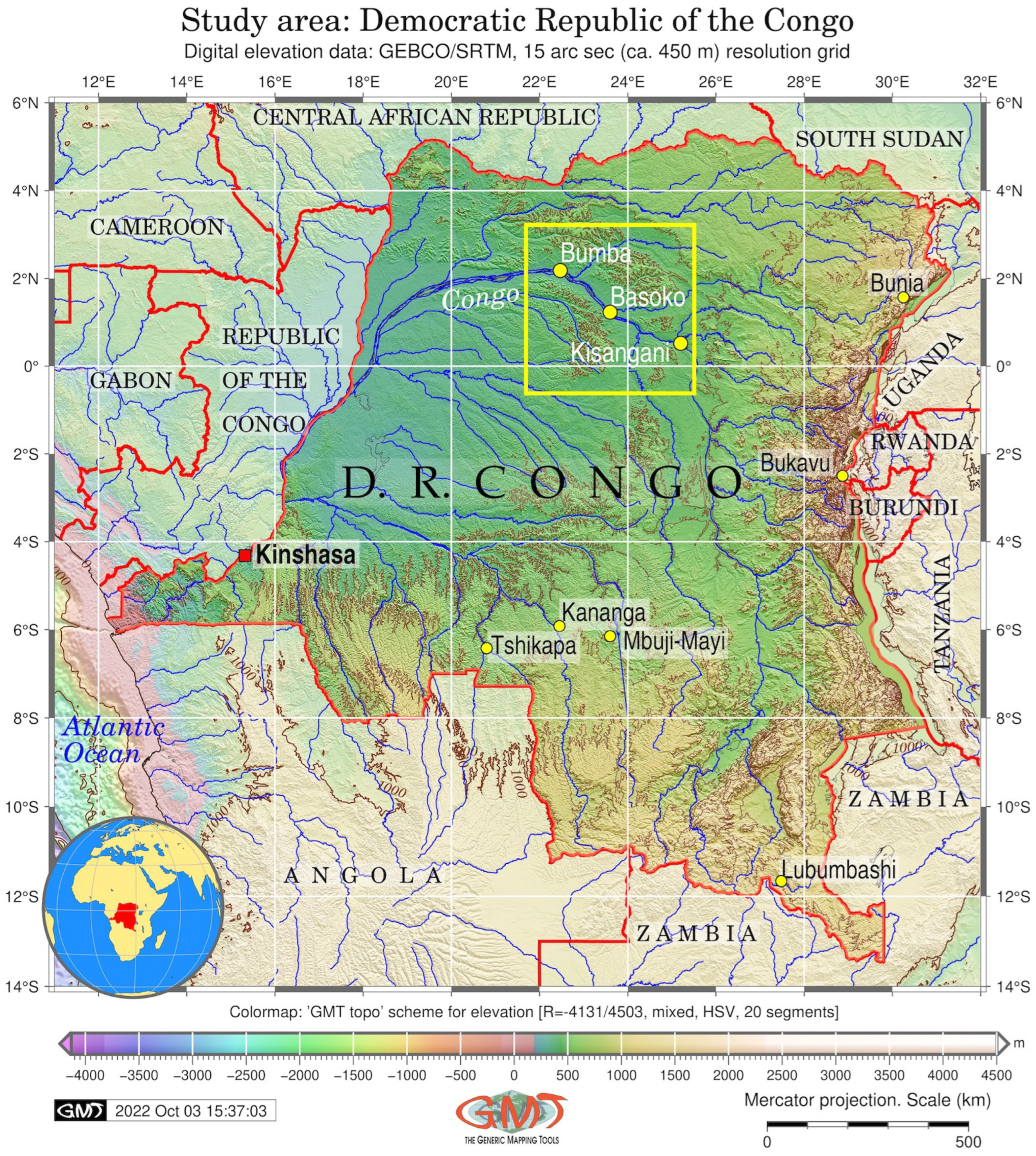
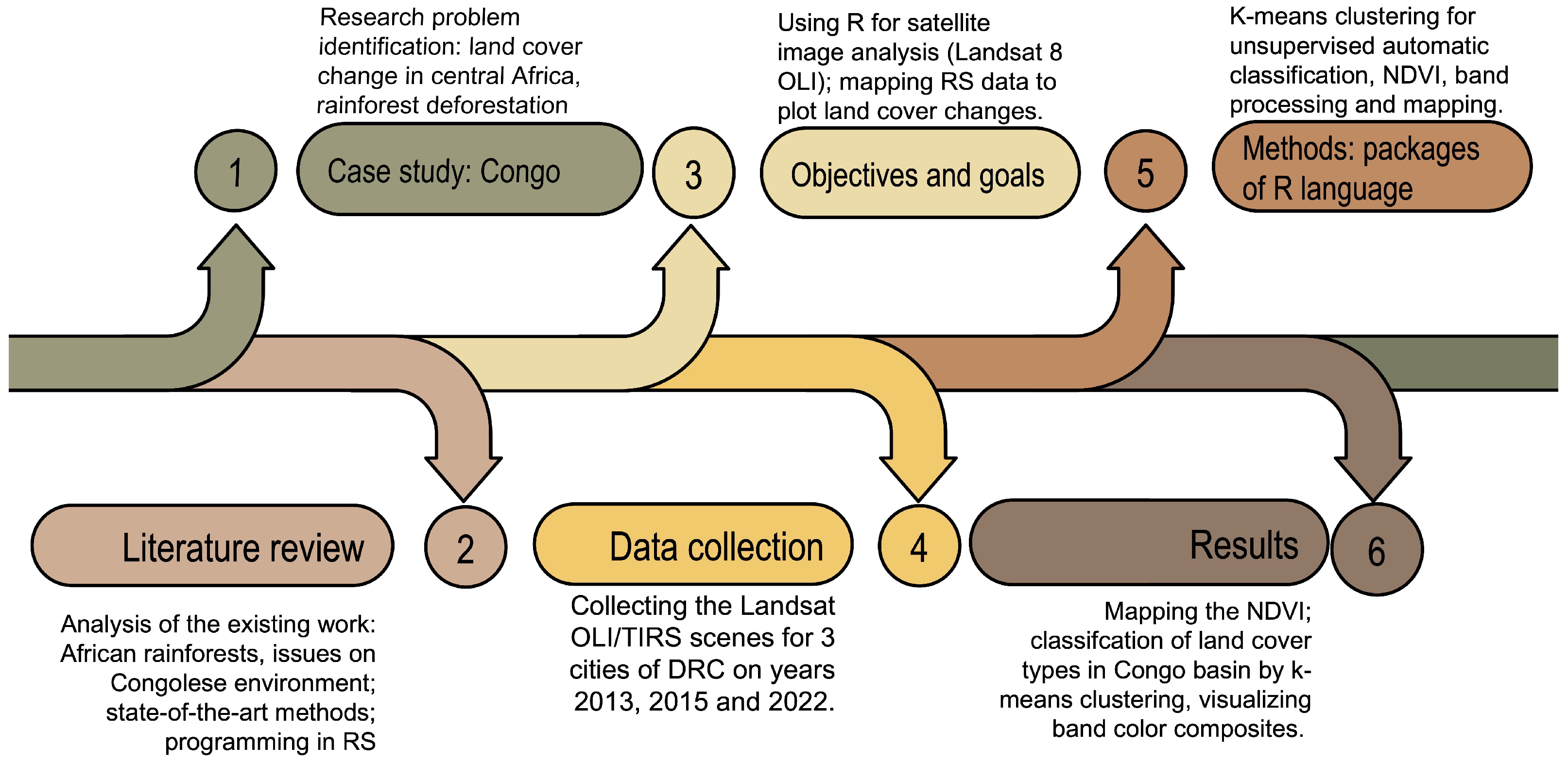
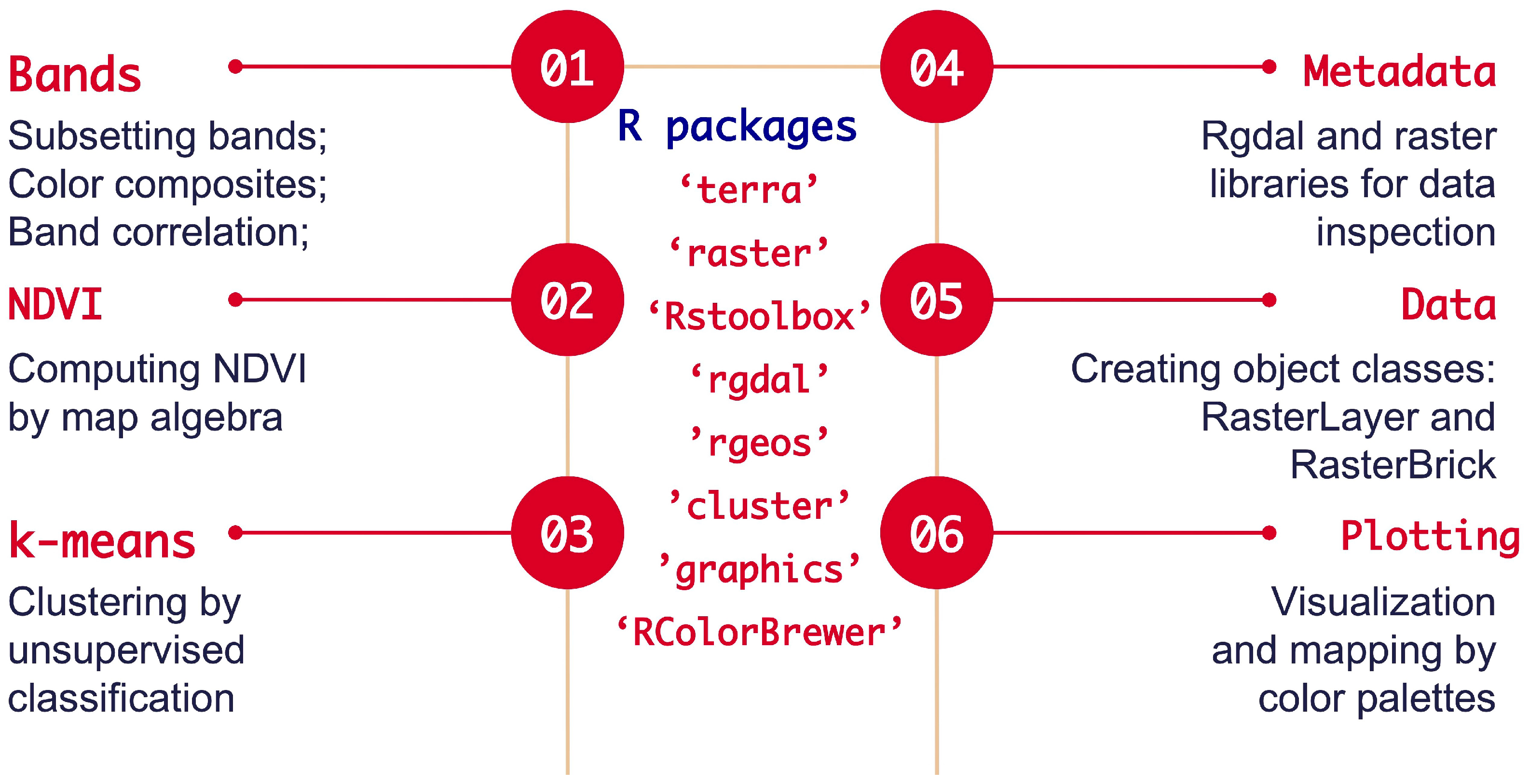
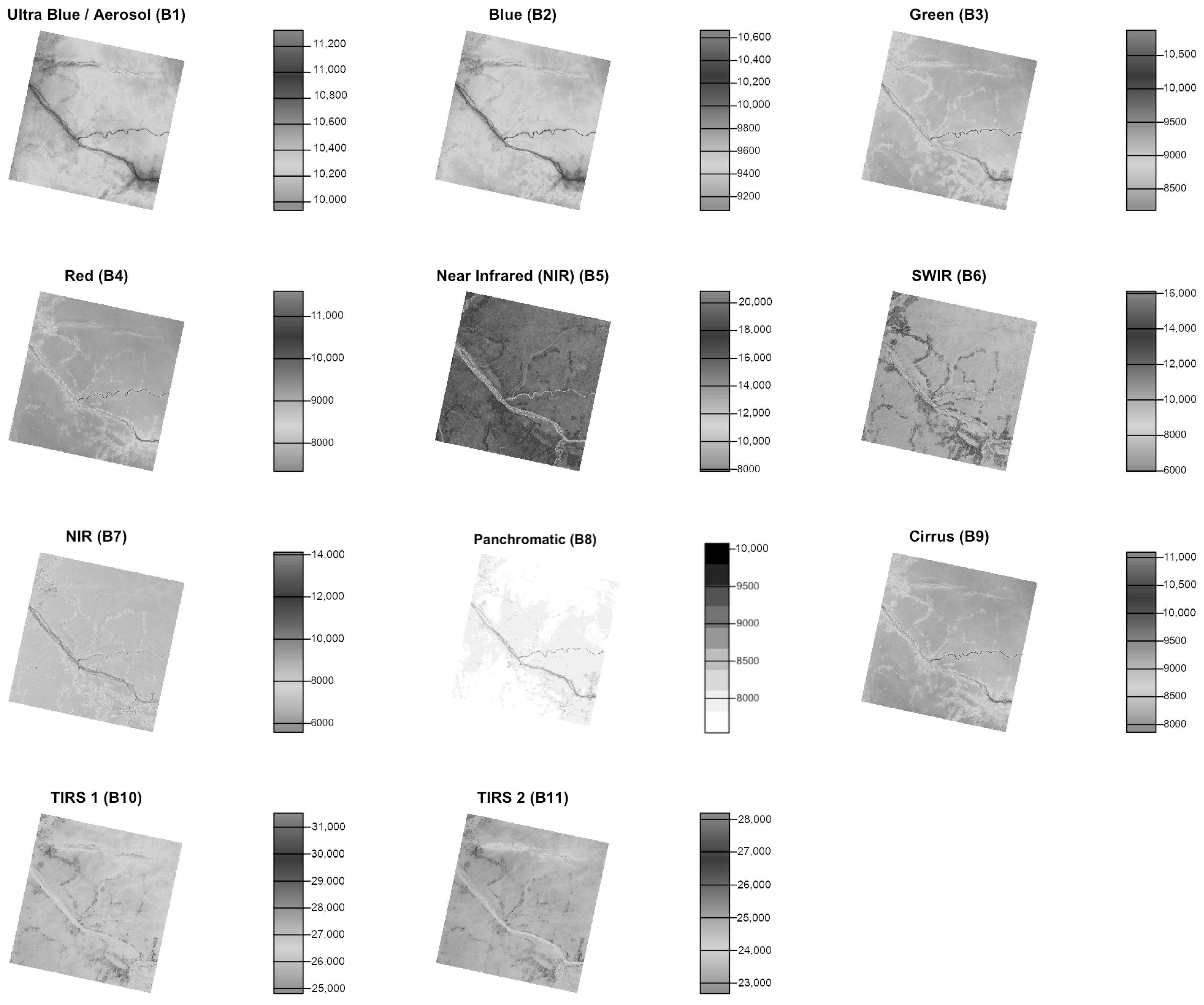
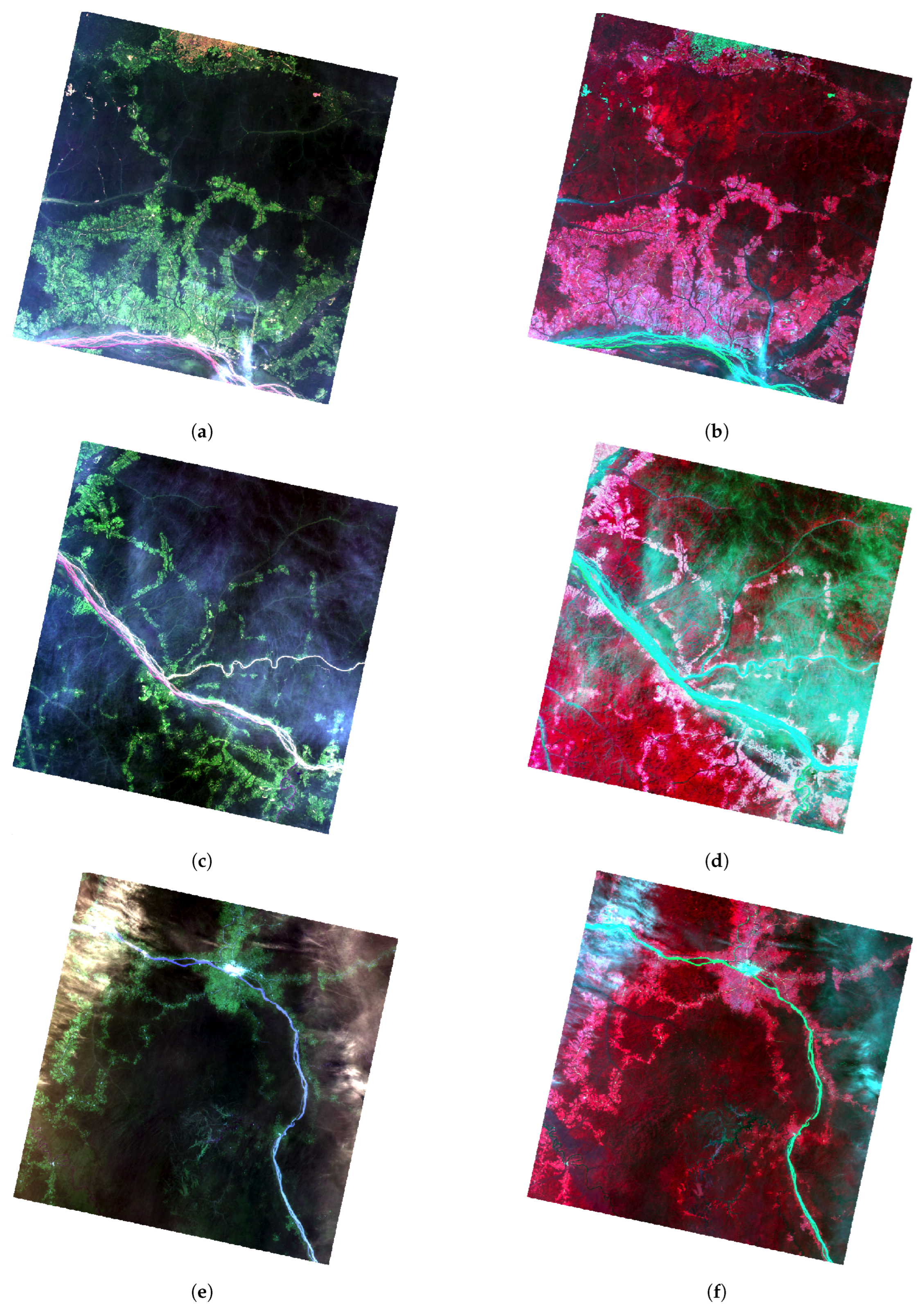
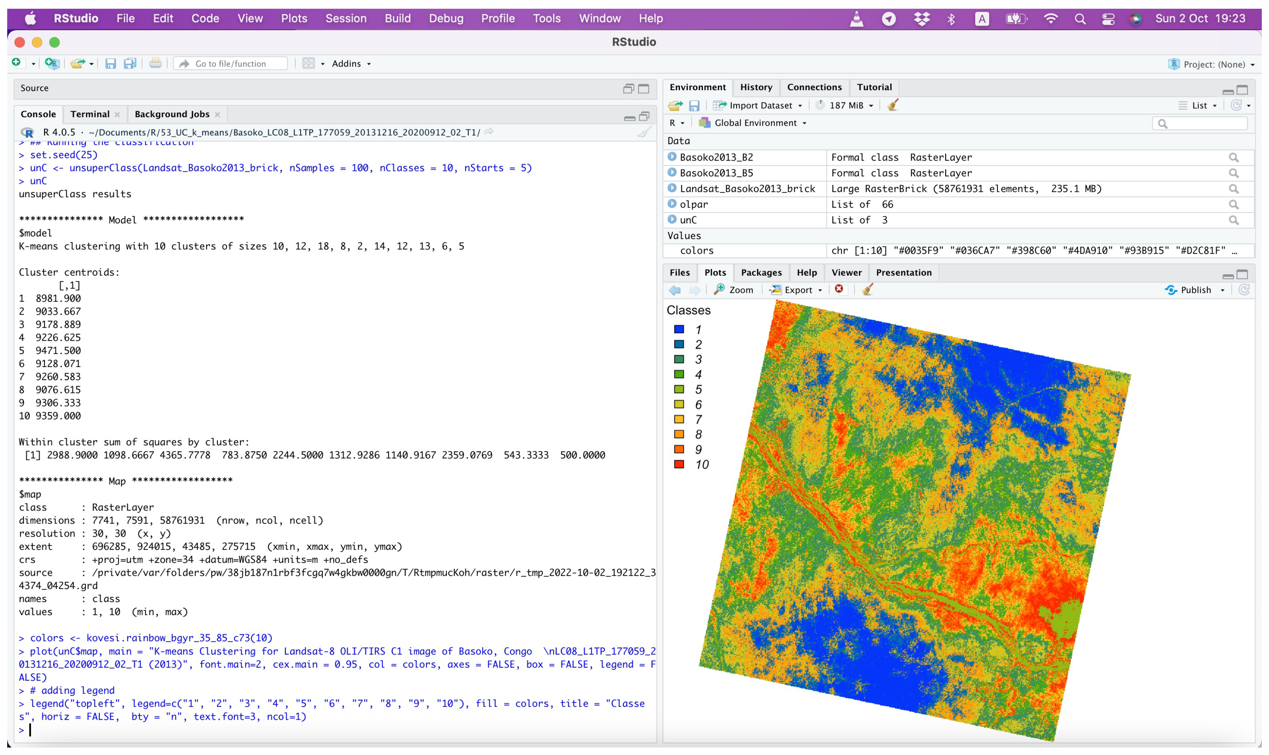
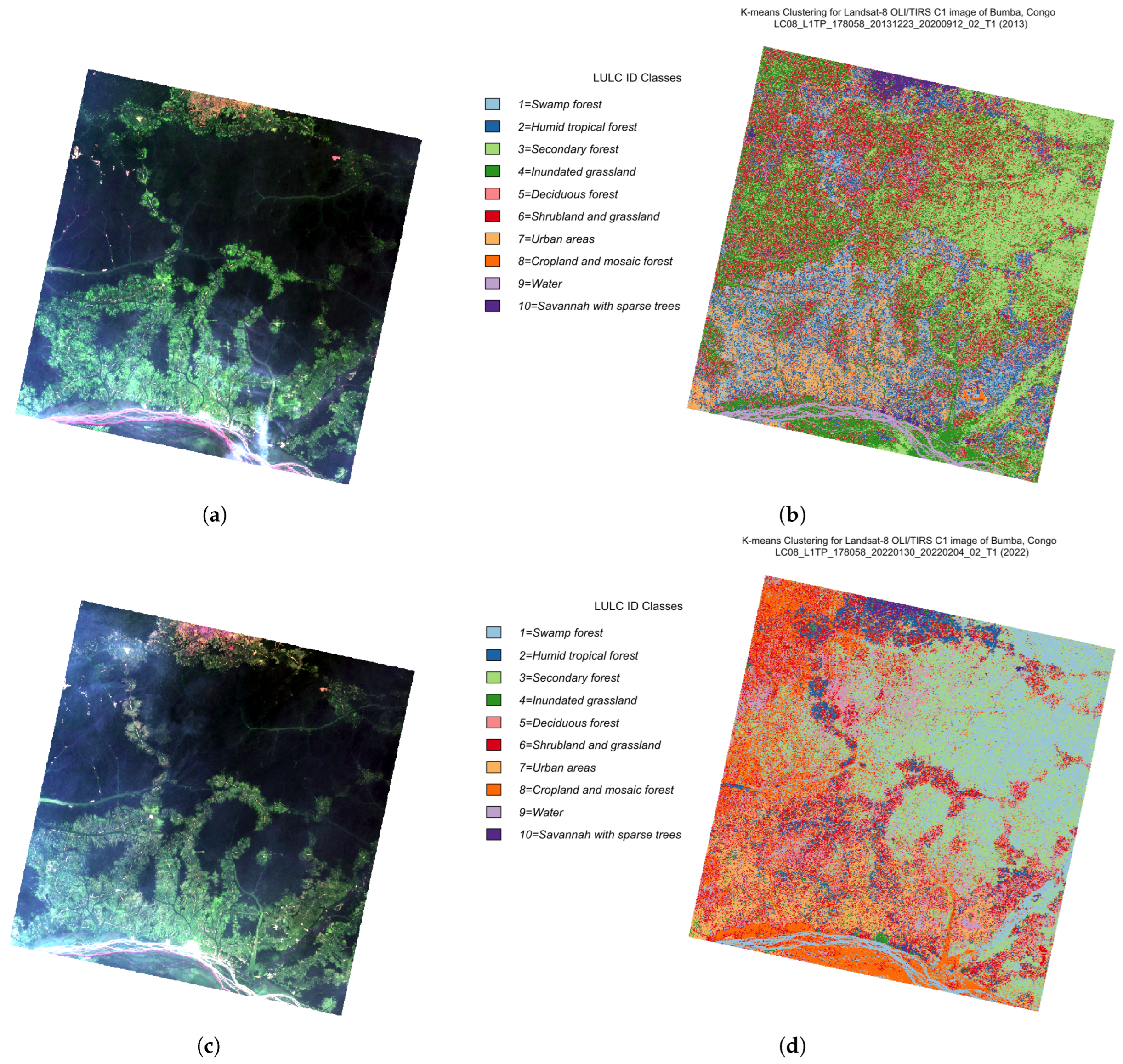
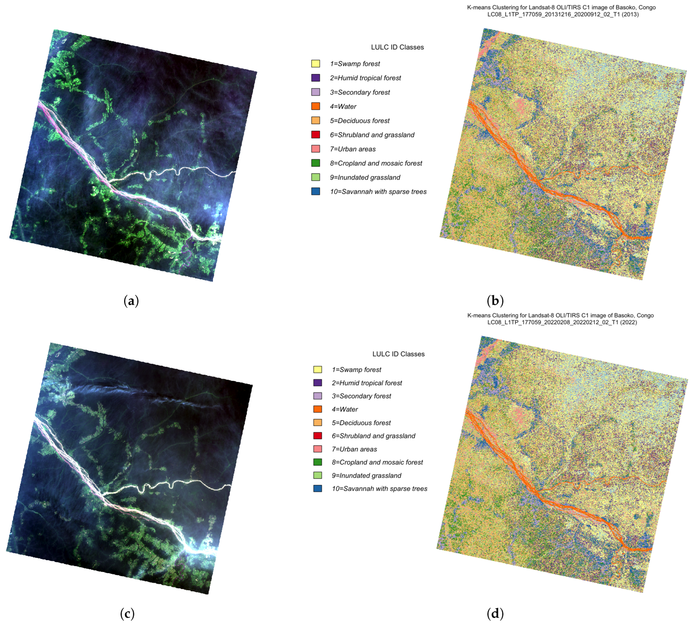
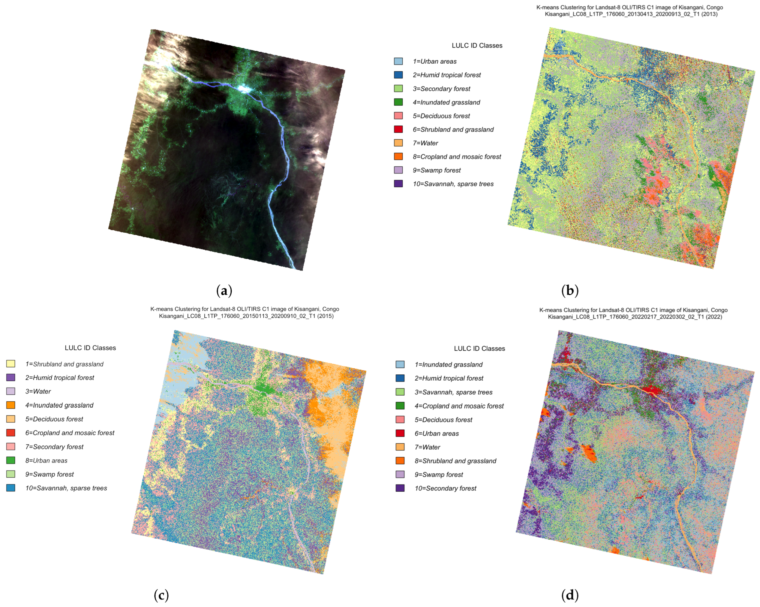
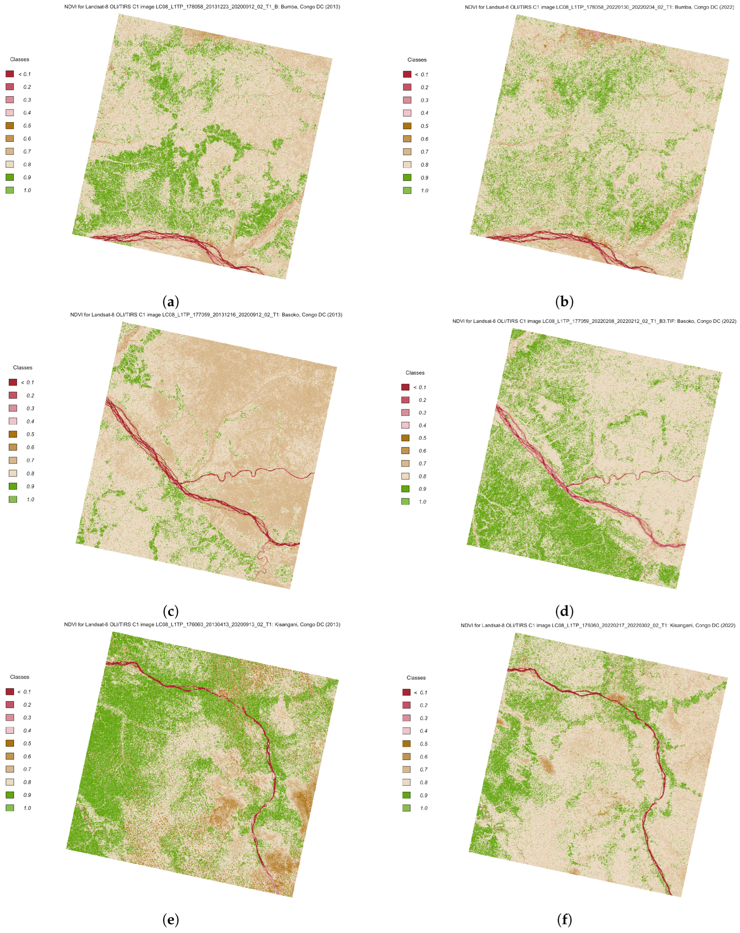
Table 1.
Landsat-8 OLI/TIRS Product ID and Scene ID.
| Region, Year | Landsat Product ID | Landsat Scene ID |
|---|---|---|
| Basoko, 2013 | LC08_L1TP_177059_20131216_20200912_02_T1 | LC81770592013350LGN01 |
| Basoko, 2022 | LC08_L1TP_177059_20220208_20220212_02_T1 | LC81770592022039LGN00 |
| Bumba, 2013 | LC08_L1TP_178058_20131223_20200912_02_T1 | LC81780582013357LGN01 |
| Bumba, 2022 | LC08_L1TP_178058_20220130_20220204_02_T1 | LC81780582022030LGN00 |
| Kisangani, 2013 | LC08_L1TP_176060_20130413_20200913_02_T1 | LC81760602013103LGN02 |
| Kisangani, 2015 | LC08_L1TP_176060_20150113_20200910_02_T1 | LC81760602015013LGN01 |
| Kisangani, 2022 | LC08_L1TP_176060_20220217_20220302_02_T1 | LC81760602022048LGN00 |
Table 2.
Main technical characteristics of the Landsat-8 OLI/TIRS imagery.
| Parameters | Basoko (2013) | Basoko (2022) | Bumba (2013) | Bumba (2022) | Kisangani (2013) | Kisangani (2015) | Kisangani (2022) |
|---|---|---|---|---|---|---|---|
| Date | 16 December 2013 | 8 February 2022 | 23 December 2013 | 30 January 2022 | 13 April 2013 | 13 January 2015 | 17 February 2022 |
| TWRS P. | 177 | 177 | 178 | 178 | 176 | 176 | 176 |
| WRS Row | 59 | 59 | 58 | 58 | 60 | 60 | 60 |
| WRS Path | 177 | 177 | 178 | 178 | 176 | 176 | 176 |
| Cloudiness | 0.00 | 0.00 | 0.04 | 0.00 | 5.85 | 1.36 | 0.48 |
| UTM Zone | 34 | 34 | 34 | 34 | 35 | 35 | 35 |
Abbreviations used in Table 2: SA—sun zzimuth. Date stands for the acquisition date of the scene; GCP Ver.—GCP version; TWRS P.—target WRS path; GCP Mod.—GCP model; GRMSEM—geometric RMSE model.
Publisher’s Note: MDPI stays neutral with regard to jurisdictional claims in published maps and institutional affiliations. |
© 2022 by the authors. Licensee MDPI, Basel, Switzerland. This article is an open access article distributed under the terms and conditions of the Creative Commons Attribution (CC BY) license (https://creativecommons.org/licenses/by/4.0/).
Share and Cite
MDPI and ACS Style
Lemenkova, P.; Debeir, O. R Libraries for Remote Sensing Data Classification by K-Means Clustering and NDVI Computation in Congo River Basin, DRC. Appl. Sci. 2022, 12, 12554. https://doi.org/10.3390/app122412554
AMA Style
Lemenkova P, Debeir O. R Libraries for Remote Sensing Data Classification by K-Means Clustering and NDVI Computation in Congo River Basin, DRC. Applied Sciences. 2022; 12(24):12554. https://doi.org/10.3390/app122412554
Chicago/Turabian StyleLemenkova, Polina, and Olivier Debeir. 2022. "R Libraries for Remote Sensing Data Classification by K-Means Clustering and NDVI Computation in Congo River Basin, DRC" Applied Sciences 12, no. 24: 12554. https://doi.org/10.3390/app122412554
Note that from the first issue of 2016, this journal uses article numbers instead of page numbers. See further details here.