
Common-Mode Driven Synchronous Filtering of the Powerline Interference in ECG


Institute of Biophysics and Biomedical Engineering, Bulgarian Academy of Sciences, Acad. G. Bonchev Str. Bl. 105, 1113 Sofia, Bulgaria
*
Author to whom correspondence should be addressed.
Appl. Sci. 2022, 12(22), 11328; https://doi.org/10.3390/app122211328
Submission received: 18 October 2022
/
Revised: 29 October 2022
/
Accepted: 5 November 2022
/
Published: 8 November 2022
(This article belongs to the Special Issue Recent Advances in Biomedical Image and Signal Processing)
Abstract
:Featured Application
This work presents common-mode driven synchronous filtering (SF) of powerline interference (PLI) by a software demodulator-remodulator concept. SF is shown to be robust against deviations in PLI amplitude, frequency, and phase with calibration and physiologic ECG signals. The presented SF algorithm is generalizable to different biopotential acquisition settings via surface electrodes (electroencephalogram, electromyogram, electrooculogram, etc.) and can benefit many diagnostic and therapeutic medical devices.
Abstract
Powerline interference (PLI) is a major disturbing factor in ground-free biopotential acquisition systems. PLI produces both common-mode and differential input voltages. The first is suppressed by a high common-mode rejection ratio of bioamplifiers. However, the differential PLI component evoked by the imbalance of electrode impedances is amplified together with the diagnostic differential biosignal. Therefore, PLI filtering is always demanded and commonly managed by analog or digital band-rejection filters. In electrocardiography (ECG), PLI filters are not ideal, inducing QRS and ST distortions as a transient reaction to steep slopes, or PLI remains when its amplitude varies and PLI frequency deviates from the notch. This study aims to minimize the filter errors in wide deviation ranges of PLI amplitudes and frequencies, introducing a novel biopotential readout circuit with a software PLI demodulator–remodulator concept for synchronous processing of both differential-mode and common-mode signals. A closed-loop digital synchronous filtering (SF) algorithm is designed to subtract a PLI estimation from the differential-mode input in real time. The PLI estimation branch connected to the SF output includes four stages: (i) prefilter and QRS limiter; (ii) quadrature demodulator of the output PLI using a common-mode driven reference; (iii) two servo loops for low-pass filtering and the integration of in-phase and quadrature errors; (iv) quadrature remodulator for synthesis of the estimated PLI using the common-mode signal as a carrier frequency. A simulation study of artificially generated PLI sinusoids with frequency deviations (48–52 Hz, slew rate 0.01–0.1 Hz/s) and amplitude deviations (root mean square (r.m.s.) 50–1000 μV, slew rate 10–200 μV/s) is conducted for the optimization of SF servo loop settings with artificial signals from the CTS-ECG calibration database (10 s, 1 lead) as well as for the SF algorithm test with 40 low-noise recordings from the Physionet PTB Diagnostic ECG database (10 s, 12 leads) and CTS-ECG analytical database (10 s, 8 leads). The statistical study for the PLI frequencies (48–52 Hz, slew rate ≤ 0.1 Hz/s) and amplitudes (≤1000 μV r.m.s., slew rate ≤ 40 μV/s) show that maximal SF errors do not exceed 15 μV for any record and any lead, which satisfies the standard requirements for a peak ringing noise of < 25 μV. The signal-to-noise ratio improvement reaches 57–60 dB. SF is shown to be robust against phase shifts between differential- and common-mode PLI. Although validated for ECG signals, the presented SF algorithm is generalizable to different biopotential acquisition settings via surface electrodes (electroencephalogram, electromyogram, electrooculogram, etc.) and can benefit many diagnostic and therapeutic medical devices.
1. Introduction
Recording myocardial electrical activity, namely, an electrocardiogram (ECG), through electrodes placed on the human body skin is a standard clinical diagnostic practice for noninvasive screening of the heart status and timely detection of rhythm and conduction disturbances [1,2]. The human body is a volume conductor, which collects interference currents like antennas. The power grid is the major source of interference currents. The capacitance between the body and the ground (neutral wire) is considered to be about 200 pF. The coupling capacitance to the live wire is usually about 2 pF [2,3]. The maximum values of these stray capacitances have been measured up to 4 nF and 5 pF [4,5]. These capacitive couplings conduct a powerline interference (PLI) current of nearly 200 nA that flows through the body to the ground. PLI currents partially pass through the electrodes directed to the signal ground of the amplifier. Therefore, bioamplifiers with a high common-mode rejection ratio (CMRR) are demanded to prevent the voltage drop to the common-mode input impedances. The unshielded leads are a kind of antenna collecting PLI currents. In highly isolated front ends, they pass the electrodes in a direction toward the earth via the body capacitance. Finally, the total amount of PLI currents flowing via electrodes is multiplied by the electrode impedance imbalance, thus producing the differential PLI voltage drop [6]. This is adversely amplified along with the useful ECG signal and then has to be filtered by analog or digital band-rejection filters.
The analog notch filters are the simplest and most routinely applied PLI suppression techniques. Due to their transient response effect, the impulse response has an oscillatory behavior [7], which appears as ringing artifacts in ST segments after sharp QRS transitions [8,9]. Furthermore, they cause attenuation of the signal components in the stop band around the central frequency (50 or 60 Hz), thus potentially distorting diagnostic ECG components. Contemporary biomedical devices contain analog-to-digital converters (ADC) and microcontrollers (MCU) that allow the application of efficient algorithms for digital filtering, combined with artificial intelligence for feature extraction and diagnostic interpretation [10]. The requirements for the ADC resolution and sampling rate are demanding for precise numerical computations, such that 1 µV/LSB with a sampling frequency higher than 1 kHz is a common practice when processing high-resolution ECG signals.
The simplest and most common options for PLI suppression are the low-pass averaging digital comb filters with a first notch at the PLI main harmonic [10]. These are also known as averagers, smoothers, or moving-average, rolling-average, or running-mean filters. In spite of their simple structure and linear phase response, such filters limit the signal bandwidth and can significantly attenuate important frequency components. A repeatable filtration–addition–subtraction approach can partially improve their high-frequency response [11]. While PLI frequency can vary, an adaptive moving-average filter with a variable length could lower the output filter error [12].
More complex are the infinite impulse response (IIR) filters, which have a simple structure but provide a non-linear phase response, and for minimal distortions should have a high Q and slow reaction time [13]. Implementing high Q leads to reduced performance when PLI frequency varies from its nominal value. If the filter does not have a comb response, a multiple notch IIR filtering could cancel the higher PLI harmonics [14]. Common ECG signal distortions are, however, caused by the transient impulse response of high-Q IIR filters, majorly triggered by the QRS complexes as the steepest parts of the ECG signal. The resulting damped oscillations and ringing artifacts in ST segments could be suppressed if the ECG is preliminarily low-pass filtered by a moving-average filter [15].
High-Q finite impulse response (FIR) comb filters benefit from a linear phase response but introduce a large group delay. The concept of averaging several differences between samples shifted in multiple PLI periods could gain a high-Q response at the cost of a large amount of data [16]. Adaptive tunable notch FIR filters could increase the performance when PLI frequency deviates [17].
A smart PLI filtering approach is the subtraction procedure [18,19], which accurately measures the PLI waveform in linear or isoelectric signal segments and subtracts this estimation in non-linear segments. Its advantage for the rejection of all PLI harmonics has been extensively studied for ECG signals; however, it is not applicable to other biosignals without linear segments. The proper operation requires accurate detection of signal linearity, and the sampling rate should be a multiple of the PLI frequency. While this is not the common case, many additional calculations are needed [20]. Novel modifications of the subtraction procedure for high-sampled signals have been recently reported [21].
Adaptive filters are very popular for PLI filtering. They change their characteristics and adapt to the filtered noise [22,23]. Such filters operate like a servo system with negative feedback, which minimizes a given error function while optimizing the filter coefficients and extracting the noise. Usually, these filters minimize the output signal power by minimizing the mean squared error (MSE), and such an approach of iteratively modifying the filter coefficients using the MSE is referred to as a least-mean-square (LMS) algorithm [24,25,26]. Various modifications of a recursive least-squares algorithm [27], block-based time–frequency domain adaptive filters [28], or cascaded multistage adaptive structures [29] present improved efficiency.
Digital lock-in techniques for adaptive PLI extraction have been introduced in [30]. The lock-in techniques are based on a quadrature amplitude demodulation (QAD) used to estimate the in-phase and quadrature PLI components. As soon as the in-phase and quadrature components are found, the PLI is orthogonally synthesized as a sine wave, which is subtracted from the input signal. A QAD frequency estimation scheme could be used to control a notch filter for precise PLI suppression [31].
Frequency domain filtering of PLI is based on Fourier transforms [32,33,34]. The signal is converted from the time into the frequency domain by fast Fourier transform (FFT), and after rejection of noise spectral components it is restored back into the time domain by inverse FFT (IFFT). Such FFT/IFFT filtering takes up a lot of computing resources and is usually implemented in special digital signal processing (DSP) chips or field-programmable gate arrays (FPGA). Similar in complexity is the wavelet decomposition, which transforms the signal into the time–frequency wavelet domain by a set of coefficients and mother wavelets, defining frequency sub-bands. After zeroing wavelet detail coefficients in the noise sub-bands, the signal is reconstructed out of the wavelet domain [35,36].
A common disadvantage of most PLI filters is their reduced efficiency when PLI frequency deviates from the nominal value. Under such conditions, the sampling rate is not a multiple of the PLI frequency, so the latter does not match the filter notch frequency. Other disadvantages are the introduced group delay and the increased complexity, which interferes with their real-time processing application. A recently developed and validated impedance balancing approach overcomes these problems [37]. It syncs to the actual PLI frequency by a dedicated software phase-locked loop (SPLL), which uses the common-mode voltage as a synchronizing reference [38,39]. PLI is canceled by an automatic summation of the differential signal with a part of the common-mode signal in a mixed analog–digital concept. The experimental results in [37] validated the efficiency of synchronous PLI filtering, which has been our main motivation to further explore the potential of digital synchronous PLI filtering with a new biopotential readout circuit design.
This study aims to present a novel PLI filtering approach that surpasses all existing methods. The biosignals are acquired by an original biopotential readout circuit wherein both the common-mode and the differential-mode signals are processed together. The implemented digital signal processing features with an innovative synchronous filtering (SF) concept, based on a digital demodulator–remodulator algorithm for the filtering of the differential-mode signal, wherein the common-mode signal is used as a synchronizing reference. The amplitude of the common-mode signal is stabilized by a tricky open-loop all-digital automatic-gain-control (AGC) stage, making possible the SF operation without a dedicated SPLL. The presented closed-loop SF algorithm is analyzed in detail. The SF approach is validated by an exhaustive test concept, involving clinical and synthesized ECG signals and PLI with variable amplitude and frequency.
2. Materials and Methods
2.1. ECG Databases
2.1.1. CTS-ECG Database
Artificially generated ECG-like signals with well-defined amplitude–time characteristics by mathematical functions were taken from the test atlas of the “Conformance Testing Services For Computerized Electrocardiography”, namely, the CTS-ECG calibration and analytical database [40]. It was originally sampled at 500 Hz in the amplitude range of ±5 mV and various amplitude and interval duration settings of waves similar to P, Q, R, S, or T (heart rate from 60 to 150 bpm, ST amplitudes of ±200 μV, configuration of RS, R, Q, QR, QRS, short RS). A total of 16 files (1 ECG lead) were used in the CTS-ECG calibration dataset, namely, CAL05000, CAL10000, CAL15000, CAL20000, CAL20002, CAL20100, CAL20110, CAL20160, CAL20200, CAL20210, CAL20260, CAL20500, CAL20502, CAL30000, CAL40000, CAL50000. Three files were used from the CTS-ECG analytical database with realistic and different waveforms in 8 ECG leads (I, II, V1-V6), namely, ANE20000, ANE20001, ANE20002. This database has been included in the IEC 60601-2-25:2011 standard [41] for ensuring the optimum performance of the hardware circuits and software programs in reliable diagnostic electrocardiographs, addressing ECG filters and automated amplitude and interval measurement algorithms.
2.1.2. PTB Diagnostic ECG Database
For the test purposes, clinical ECG signals included in the PTB Diagnostic ECG Database [42] from the PhysioNet archive [43] were used. Originally, the database contained 549 conventional 12-lead resting ECGs, which were digitized with a sampling rate of 1000 Hz, resolution of 0.5 μV/LSB, and 16-bit ADC, including healthy controls and various pathologies for myocardial infarctions (MI), arrhythmias, heart blocks, myocardial hypertrophy, etc. Most of the recordings, however, contained noises induced during the primary ECG acquisition stage and, therefore, were unusable for benchmark testing of filters. In such testing, the filter could potentially suppress the genuine noisy components, which would be read as generating distortions. Therefore, before the study, the noise content of the PTB Diagnostic ECG Database was automatically estimated in the low-frequency band (selective for baseline wander) and high-frequency band (selective for powerline and muscle noises), and only low-noise recordings were considered eligible for general benchmark testing of filters. The low-frequency band was estimated at the output of a linear pass-band filter (0.3–0.5 Hz) to not exceed 25 μV in all 12 ECG leads. The high-frequency band was estimated at the output of a linear-slope finite impulse response (FIR) filter (30–48 Hz)—order 182, equiripple (negligible in pass and stop bands)—that does not produce ringing as an effect after steep QRS. The maximal tolerated high-frequency content outside QRS complexes was limited to 12.5 μV in all 12 ECG leads. The eligible best quality records numbered 40, all used in the filter benchmark study, including: s0064lre (diagnosis: anterior MI), s0127lre (inferior MI), s0219lre (inferior MI), s0137lre (antero-septal MI), s0313lre (antero-lateral MI), s0411lre (inferior MI), s0291lre (healthy control), s0292lre (healthy control), s0006_re (diagnosis: n/a), s0154_re (palpitation, coronary heart disease, arterial hypertension), s0301lre (healthy control), s0325lre (healthy control), s0366lre (congenital complete AV block), s0374lre (healthy control), s0490_re (healthy control), s0308lre (healthy control), s0433_re (anterior MI), s0449_re (infero-lateral MI), s0452_re (healthy control), s0455_re (infero-lateral MI), s0458_re (healthy control), s0483_re (healthy control), s0460_re (healthy control), s0462_re (healthy control), s0465_re (healthy control), s0466_re (healthy control), s0471_re (healthy control), s0478_re (healthy control), s0485_re (hypertrophy, arterial hypertension), s0487_re (healthy control), s0491_re (healthy control), s0495_re (inferior MI), s0502_re (healthy control), s0504_re (healthy control), s0529_re (diagnosis: n/a), s0531_re (healthy control), s0533_re (healthy control), s0534_re (healthy control), s0552_re (healthy control), s0546_re (dysrhythmia).
2.2. Biopotential Readout Circuits with Synchronous PLI Filtering
Two simplified biopotential readout circuit concepts are shown in Figure 1. Generally, they consist of an analog front end (AFE), two ADCs, and a digital part embedding the novel SF algorithm. AFE includes at least two amplification channels for the differential- and common-mode input signals and an optional driven reference electrode (DRE) circuit. It is worth noting that DRE is a generalization of the well-known driven-right-leg circuit coming from the standard 12-lead ECG setup where the reference electrode is placed on the right leg [44]. The number of differential channels can be arbitrarily increased. For example, in a 12-lead ECG system, the differential channels are 8 (6 precordial and 2 peripheral leads), but for simplicity only 1 differential channel is shown in Figure 1. The proposed SF algorithm can be embedded in biopotential acquisition configurations with and without DRE. In systems with DRE, the common-mode signal could be taken from the DRE electrode, as shown in Figure 1a. In ground-free systems shown in Figure 1b, the AFE common-mode input impedance should be low enough to provide flowing path for both bias and interference currents and to keep the amplifier inputs within their operating range. Both differential- and common-mode channels have appropriate gain coefficients, namely, Ad and Acm, respectively. They must also have appropriate bandwidths. For example, the diagnostic ECG bandwidth of the differential channel is broad from 0.05 Hz to 150 Hz, while the bandwidth of the common-mode channel could be considerably limited within a span of a few Hertz around the fundamental PLI harmonic. Since the amplitude of the common-mode signal is uncontrollable and can vary along with the input PLI level, the common-mode gain Acm must be controllable too. We have previously proposed such an option by means of a software automatic gain control (SAGC) [45], which could be embedded either as a variable gain amplifier (VGA) in AFE or as a digital multiplier in the digital part. The amplified differential- and common-mode analog signals are digitized by two ADCs, which could be either stand-alone integrated circuits or embedded into the digital processing part. Thus, the SF algorithm can input and synchronously process the samples of both differential- and common-mode signals. Generally, depending on the specific readout circuit design, the digital SF algorithm could be embedded either in a DSP, FPGA, or in the system MCU. For mains-powered medical instrumentation, AFE must be supplied from a medical-grade power supply. AFE provides safe and reliable patient isolation by limiting the safe level of the viable mains currents, usually through optical, magnetic, or wireless signal transmission to the non-isolated part.
2.3. Synchronous Filtering Concept
Synchronous filtering is a widely used technique for carrier recovery and image rejection in radio-frequency signal processing [46]. A simplified diagram of a synchronous filter is shown in Figure 2a. It consists of a core filter enclosed by mixers [47]. Each mixer is a precision multiplier. The first one (M1) is a demodulator, the second one (M2) is a modulator, and the net result of the SF system behaves as an equivalent filter without mixers. Synchronous filtering has the functionality to accomplish some typically difficult tasks for design filters (i.e., very high-frequency, very high-Q band-pass filters) with a relatively simple core filter design [47].
The SF operation can be simply explained with the following example. Let us assume that the reference signal (VREF) is in phase with the input signal (VSIG) and both are sinusoidal waveforms, as written in Equations (1) and (2):
The output of the first mixer M1 is the product of (1) and (2), expressed by (3):
The core filter is usually a low-pass filter (LPF) with a sufficiently low cutoff frequency (f3dB); therefore, it passes the DC component and filters out the AC component with doubled frequency in (3). Thus, the SF output signal becomes:
where the gain G of the SF algorithm is expressed by (5):
When Vr = √2 = 1.414 V, the SF algorithm recovers the input signal VSIG with unity gain. The second mixer M2 is an up-converter and translates the cutoff frequency f3dB of the core filter in two sidebands around the VREF frequency (fref). Thus, the SF filter acts as a band-pass filter with a quality factor Q, given by (6):
It can be deduced from (6) that a very high Q factor can be achieved by configuring the cutoff frequency f3dB and its ratio to fref. SF algorithms have great advantages in carrier extraction and recovery. For example, let us assume that VSIG is disturbed by a spike noise and occasionally a few periods are missing. Due to the large LPF time constant, the filtered carrier (VSF) can be recovered and free of such spike noise disturbance. In order to operate with arbitrary phase differences between VSIG and VREF, an orthogonal SF architecture is conventionally used [48]. It includes two parallel SFs shown in Figure 2a, operating with quadrature reference signals. Their outputs are summed, as shown in Figure 2b. The left mixers M1 and M3 are quadrature demodulators, while the right mixers M2 and M4 are quadrature remodulators, and together all of them perform two frequency conversions. First, the spectrum of the input signal is shifted from the two sidebands around fref to the baseband, i.e., close to DC. After low-pass filtering of the demodulated spectral components, they are shifted again from the baseband to the two sidebands around fref, i.e., the spectrum is restored into the two sidebands, but the bandwidths are limited to fref ± f3dB. Thus, the quadrature SF architecture, employing quadrature demodulator–remodulator (QDR), exhibits a band-pass frequency response.
The QDR architecture was introduced about 70 years ago by Donald Weaver for the generation and detection of single-sideband radio signals [48]. We should point out some important properties of the QDR architecture. First, in case LPF core filters are missing (i.e., bypassed), Equation (7) is valid, resulting in restoration of the input signal at the QDR output by a gain Vr2, which depends neither on the DC nor AC form of VSIG:
Otherwise, in case LPF core filters are present and the input signal is a pure DC offset, then it is converted by the first mixers into sine and cosine waves with a frequency fref. The LPL core filters reduce output amplitudes (Vx) and introduce a phase lag of 90°. Further, in the second mixers, LPF outputs are again multiplied by sine and cosine waves, and their sum produces zero QDR output (VSF in Figure 2b), given the basic trigonometric identity in (8):
Therefore, it is important that LPFs have a minimum phase response, thus introducing a phase lag of 90° in their stop bands. An important effect of the QDR operation is the suppressed input DC offset. In a similar manner, according to the basic trigonometric identity:
the second harmonic, produced by the useful differential signal VSIG from Equation (1) does not generate a third harmonic but can produce only a fundamental harmonic.
While QDR is connected in the negative feedback, its band-pass response is subtracted from the input signal and is converted into a band-stop response for the forward path, thus rejecting the PLI. Such a closed-loop synchronous filter for PLI extraction with QDR in the negative feedback is shown in Figure 3a. QDR estimates the PLI error appearing in the demodulator output signals and automatically changes the amplitude and phase of the synthesized PLI in order to minimize the estimated error. The operation of the closed-loop SF concept from Figure 3a is illustrated in Figure 3b. It can be seen that after settling of the in-phase and quadrature control signals for the remodulator, namely, I and Q, the PLI is canceled. The longest transient processes of I and Q (settling over less than 0.2 s) is normally observed after turning on the filter, hereafter referred to as the start-up time.
The closed-loop architecture must ensure automatic zeroing of the steady-state residual PLI. Therefore, the loop filter must have infinite gain for low frequencies and DC, and low gain for high frequencies, which can ensure a stable response. The digital integrator is the main gain block in servo control. The loop filter must contain at least one integrator. The transfer function of the loop filters LF(z) used in [37] is given by (10):
Equation (10) includes the coefficient ki, two cascaded averagers (one PLI period), and a digital integrator. We can further consider the stability of the closed-loop system in detail by using (10) as an example for LF(z). The two averagers in (10) are optional, and, if omitted, the stability constraints are simplified. Note that the digital integrator behaves as an ideal integrator whose frequency response has an infinite DC gain and roll-off of –20 dB/dec. Thus, its infinite DC gain minimizes the steady-state error within ±1 LSB. The sampling frequency is set up to Fs = 2 kHz and corresponds to an integration time constant τi = 1/Fs = 0.5 ms or to an integrator unity-gain frequency, UGF = 1/(2πτi) = 318 Hz. For stable operation and filtering of the PLI fundamental harmonic, the integrator time constant must be expanded to compensate for the 20 ms group delay of the two averagers. As the outputs of the averagers are divided by the coefficient ki, the UGF of the integrator is shifted to DC, i.e., the time constant of the integrator is incremented. It should be noted that the frequency response of an ideal integrator can be determined from only one point, e.g., its UGF. The integrator roll-off was known and was 1/f or −20 dB/dec. The coefficient ki determines the overall stability of the system. It must be carefully tuned to ensure a stable operation with fast transient response and short start-up time. Considering that the cutoff frequency of the two averagers is much higher than the bandwidth of the closed-loop response, we can neglect the averagers’ transfer function. Thus, (10) could be expressed by means of Fs and the integrator 1/f roll-off, as shown in (11):
The coefficient ki can be regulated by the loop gain (LG) of the QDR servo loop. The loop gain determines the stability of the control system with a negative feedback. In case LG = 1 (0 dB), the crossover frequency settles the loop bandwidth and defines −3 dB cutoff frequency of the closed-loop response (f3dB). Deduced from Figure 3, the SF loop gain is expressed by (12):
Replacing G and kLF in (12) by Equations (5) and (11), LG becomes:
Equation (13) shows that the LG of the SF algorithm is proportional to the squared amplitude of VREF. For a constant closed-loop bandwidth and constant speed of the closed-loop response, the product Vr2ki should keep constant, i.e., when Vr changes, the coefficient ki should change accordingly. For example, when Vr is increased two times, the coefficient ki should be decreased four times to maintain the same stability reserve. Equalizing (13) to unity, the cutoff frequency f3dB of the closed-loop response could be found:
The two averagers have the same −3 dB cutoff frequency (fc = 16 Hz), introducing a 20 ms group delay. If f3dB is much lower than fc, e.g., let us say ten times, it guarantees a stable operation with a phase margin of about 90°. In Equation (14), we could substitute: Vr = 200 LSB, ki = 2−23, Fs = 2 kHz, thus estimating the closed-loop response at f3dB to be about 0.7 Hz. The exact phase margin of the closed-loop response can be calculated taking into account that the two averagers are linear-phase (constant group delay) filters. The group delay of 20 ms corresponds to 360° phase lag at 50 Hz. Thus, the phase lag of the two averagers at 0.7 Hz can be calculated using the rule of three, i.e., the phase lag at 1 Hz is 360°/50 Hz = 7.2°/Hz, and at 0.7 Hz it is 0.7 Hz × 7.2°/Hz ≈ 5°. Thus, taking into account that the integrator has a constant phase lag of 90°, the actual phase margin of the closed-loop system is just 90° − 5° ≈ 85°. The crossover frequency f3dB has a reserve to be increased up to five times and can preserve a stable response within a phase margin of 65°. The loop gain LG(z) is simulated for Vr = 200 LSB, ki = 2−23, and Fs = 2 kHz, and the simulated magnitude and phase responses are shown in Figure 4. These simulations confirm the detailed analysis of the stability of the system.
Replacing f3dB = 0.7 Hz and fref = 50 Hz in Equation (6), the quality factor of the SF algorithm is estimated to be Q = 35.7. Further decrement of ki would lead to a higher Q but also to a slow reaction time. Note that 0.7 Hz corresponds to a time constant of 0.23 s and to a settling time from 10% to 90% of 2.2 × 0.23 s ≈ 0.5 s, which is a reasonable start-up time. Further, the coefficient ki should be selected with a tradeoff between Q and the limited speed of the closed-loop response. For sine wave mixing, as in our case, the two averagers are optional, and if they are not included, the phase margin of the system would always be 90° in a large variation in ki, allowing higher values of ki to be selected. For example, if ki is incremented four times, i.e., ki = 2−21, the Q factor becomes: Q = 35.7/4 ≈ 9.
2.4. Automatic Common-Mode Gain Control
The amplitude of the common-mode voltage VREF (Figure 2) corresponds to the actual PLI level and can vary in a wide range depending on the stray capacitances of the body to the power grid and earth. It depends on the physical position of the body and its proximity to the mains-powered household appliances. Thus, VREF amplitude must be stabilized by AGC to remain independent of the PLI amplitude. A closed-loop software AGC has been previously developed to stabilize the amplitude of the common-mode voltage, used for SPLL synchronization to the line frequency [37,45]. Generally, the gain control element could be implemented either with digitally controlled analog circuits (e.g., multiplying digital-to-analog-converters (DACs), digital potentiometers, analog switches, and opamps in the AFE) or with a digital multiplier in the digital part. The major advantage of the closed-loop AGCs is their ability to minimize some deficiencies of the multiplier transfer function. The accuracy of the digital multiplier depends on the digital word of the multiplicands, i.e., on the ADC resolution. Because of the ideal transfer characteristics of the digital multipliers and detectors, the entire AGC could be implemented in the digital part, and thus to have an all-digital implementation. The simplest AGC has the open-loop architecture shown in Figure 5a. It relies on the ideal transfer characteristic of the digital multiplier. The major advantages of the open-loop AGC are related to the stable control system as well the independent settling time from the input signal level. The settling time is determined only by the settling time of the implemented low-pass filter (LPF) [49].
The open-loop AGC operates as follows. Assuming that VREF has a sinusoidal waveform expressed by (2), the output of the low-pass filter (VLPF) equals the averaged absolute value of VREF. Thus, the AGC output VAGC can be expressed by (15), where VREF is substituted by (2):
From Equation (15), it is clear that the amplitude Vr drops, and the stabilized amplitude depends only on the target value Vtar. The latter should be selected taking into account the introduced π/2 gain. For example, if the stabilized VAGC amplitude is 200 LSB (1 LSB corresponds to 1 µV), Vtar should be preset to 128 LSB. For proper operation of AGC, any VREF offset should be removed with a high-pass pre-filter. An appropriate digital solution is a simple first difference filter (FDF), which removes the offset and passes the PLI fundamental frequency at a unity gain. Its transfer function for a sampling rate of 2 kHz is given by (16):
Just after turning on the system, the LPF output starts from zero, which produces very high values in AGC output VAGC. Therefore, an output limiter is added to truncate the output to ±Vlim, where the limiter threshold is equal to the nominal peak value of VAGC. Thus, at start-up, VAGC begins as a rectangular wave, which automatically converts to a trapezoidal wave, then to a truncated sine wave, and finally when LPF is settled it becomes a pure sine wave, according to the start-up simulations in Figure 5b. It should be noted that the open-loop AGCs are also known as feed-forward AGCs; however, the published architectures require complex computations with logarithmic and exponential functions [50]. The presented open-loop AGC has the advantage of being much simpler. The open-loop AGC architecture is based on the ideal transfer characteristics of the implemented digital blocks, such as digital detectors and multipliers. When a peak detector is used, AGC can operate even without LPF. However, we considered rectification and LPF as a noise-robust pre-processing stage for computation of the averaged absolute value of the signal instead of the simplest design with a single peak detector.
2.5. Optimization of SF Architecture for PLI Suppression in ECG Signals
Although the presented SF principle is fundamental, the SF architecture was further optimized for the specific application for PLI filtering in ECG signals. The implementation and optimization of the digital SF algorithm was performed in Matlab 2020b (MathWorks Inc., Natick, MA, USA) using artificial and clinical ECG signals from CTS-ECG and PTB databases, respectively. The proposed optimal architecture of the SF filter is shown in Figure 6. Both inputs VSIG and VREF were considered at a sampling frequency Fs = 2 kHz, which is higher than the original ECG databases. Therefore, all ECG signals at VSIG input were preliminarily upsampled using the Matlab function resample(). The reference input VREF is originally generated as a sinusoidal wave at 2 kHz sampling rate. The branch for PLI estimation includes a simple FDF band-pass filter with a transfer function (16). FDF has a unity gain response for the PLI frequency. It removes the DC offset and differentiates QRS complexes. Next, QRS limiter is necessary to cut extreme signal amplitudes, such as QRS complexes and high T waves exceeding a certain amplitude threshold. The threshold of the limiter is adaptively defined as follows. The absolute value of the signal at the FDF output is processed in a window of 10 ms (half PL period), and the maximum value is measured. In the next step, the extracted maximal values are averaged in a window of 50 ms in order to remove accidental spike artifacts. Finally, the averaged values are evaluated within a window of 200 ms (chosen to exceed the longest QRS duration). The minimum value is deduced and used as the positive and negative thresholds of the QRS limiter, thus being adapted to the current PLI level. The QRS limiter does not introduce group delay in the loop. It just limits the amplitude and helps to reduce the QRS influence on the demodulated signals fed to the two integrators in the loop filter. The loop filter is simplified and the two averagers are removed. It consists only of an integrator and a stability coefficient ki. If we assume ki = 2−21, the Q factor of the SF filter would be Q ≈ 9, rejecting a bandwidth of ±2.8 Hz around the PLI frequency. The added FDF and QRS limiter do not reduce the stability reserve in the closed loop, as it passes the PLI frequency by approximately zero phase shift.
The used AGC open-loop architecture has already been discussed in Section 2.3. Its stabilized VAGC amplitude was set to 200 μV as an approximation of the geometric mean between the minimal and maximal PLI amplitude in the real ECG signals, (e.g., 50 and 1000 μV, respectively), and thus it ensures symmetrical control range of AGC. LPF was implemented in AGC as a simple one PL period averager. For better filtering, the widow of this averager is adjusted when PL frequency deviates from its nominal value. Although many other LPF architectures can be used, the averager gives the fastest response. While there is no need for linear-phase LPF, the minimum-phase LPFs explained in [13] or cascaded LPFs could also be used for better filtering. It should be noted that the implemented absolute value converter doubles the PLI frequency. Thus, LPF should accurately cancel the second harmonic of PLI, otherwise it would be converted in a third harmonic at the AGC output.
2.6. Estimation of the SF Performance
The inputs of the SF algorithm are simulated as follows: the differential-mode signal VSIG is generated by superposition of an original ECG signal (without noise) and artificially generated PLI sinusoid with predefined amplitude (APLI) and frequency (fPLI), as shown in (17); the common-mode reference input VREF is generated as an artificial sinusoid with a reference amplitude (AREF), frequency (fPLI), and phase shift (φPLI) as defined in (18):
where n denotes the sample number within the duration of the signal with N samples (n = 1, 2, … N). APLI and fPLI can be linearly changing values, starting from a baseline APLI0 and fPLI0 with predefined slew rates, namely, ΔAPLI (μV/s) and ΔfPLI (Hz/s), formally written as:
When ΔAPLI = 0 μV/s or ΔfPLI = 0 Hz/s, the generated PLI sinusoid has a constant baseline amplitude or frequency, respectively.
This simulation study considered ECG and PLI signals with duration of 10 s sampled at Fs = 2 kHz, N = 20,000 samples. The following ranges of PLI parameters were defined:
- PLI with constant amplitude: APLI0 = 50–1000 μV r.m.s. computed over 10 s. The maximal setting was chosen to represent a severe realistic scenario with peak-to-peak PLI amplitude reaching 2800 μV.
- PLI with constant frequency: fPLI = 48–52 Hz, exceeding the standards for maximal mains frequency deviation in the synchronous European grid of 49.8 Hz to 50.2 Hz.
- PLI with linear amplitude change: ΔAPLI = ±(10–200) μV/s. The maximal slew rate was chosen to represent the worst realistic scenario with peak-to-peak PLI amplitude span from 0 to 4000 μV within 10 s.
- PLI with linear frequency change: fPLI = 50 Hz, ΔfPLI = ±(0.01–0.1) Hz/s. The maximal slew rate was chosen to represent the worst realistic scenario for a change in the frequency of 1 Hz over 10 s, e.g., covering a span of 49–50 Hz and 50–51 Hz.
- PLI with phase shift of the reference input VREF: φPLI = 0–360° in Equation (18).
The SF algorithm performance was estimated by means of three benchmark metrics, namely, maximal error (MAXE), root-mean-square error (RMSE), and improvement in the signal-to-noise ratio (SNRimp), as follows:
where the input SNR (SNRin) and output SNR (SNRout) are computed as follows:
MAXE and RMSE are the peak value and the root mean square value of the filter error equal to the difference between the filtered and original ECG signals. MAXE can be considered representative of the ringing noise after QRS complexes, which are typically the steepest ECG waves producing the maximal filter error. Smaller values of MAXE and RMSE imply a better performance of the filter. SNRimp is the improvement in the SNR levels between the input and the output. A higher SNRimp represents a better quality of the filtered ECG.
The statistical analysis considered the three SF performance metrics as non-normal continuous variables and reports their median values, interquartile ranges, and min–max ranges in each lead of ECG recordings in specified databases (Section 2.1) using the software package Statistica 7.0 (StatSoft Inc., Tulsa, OK, USA).
3. Results
3.1. Optimization of SF Algorithm
The optimization of the SF algorithm is focused on the choice of the stability coefficient ki = 2−μ in the loop filter (Figure 6) so that the SF could provide the best performance for different PLI parameters. The optimization process considers a range of scanned values for ki = [2−23, 2−22, 2−21, 2−20, 2−19] in the worst-case scenario, wherein PLI parameters are scaled to the maximal settings in this study with respect to the r.m.s. amplitude (1000 μV), amplitude slew rate (±200 μV/s), and frequency slew rate (0.1 Hz/s). Table 1 summarizes the three optimization strategies, namely, PLI constant (PLI with constant amplitude and frequency), PLI with linear amplitude change, and PLI with linear frequency change. While the three PLI optimization scenarios were applied with the CTS-ECG calibration database (CAL records, 1 lead, 10 s), the input SNR was estimated to be [−7.8 to −8.8 dB] (mean value), [−18 to −3 dB] (min–max range).
The optimization performance of the SF algorithm is shown in Figure 7 with respect to MAXE, RMSE, and SNRimp. The optimal setting can be read for ki = 2−21, seeking for minimization of (MAXE, RMSE) and maximization of (SNRimp) as a conciliation between the three scenarios for PLI parameter change. Higher values of ki > 2−21 are associated with a reduction in the Q factor and to higher errors during steady state, observed as higher errors for PLI with constant amplitude and frequency as well as for PLI with frequency modulation (Figure 7a,c). Lower values of ki < 2−21 are associated with an increased Q factor and a slow adaptation rate to amplitude changes, which therefore leads to higher errors for PLI with amplitude modulation (Figure 7b).
The real operation of the SF algorithm for the denoising of ECG signals with the optimal stability setting (ki = 2−21) is illustrated in Figure 8. It represents the noisy input VSIG, where the artificial ECG signal (CAL20100, heart rate of 60 bpm) is diagnostically unreadable due to the superimposed large PLI amplitude of 1000 μV r.m.s. over 10 s, according to the three PLI parameter settings in Table 1. The filter output VSF contains a denoised ECG waveform with a visually well-distinguishable P, QRS, and T waves, and isoelectric lines in all PLI parameter scenarios. The ECG distortions are estimated by the error of the filter, showing negligible values of RMSE = 1 μV, MAXE = 2 μV for constant PLI (Figure 8a) and RMSE = 1.5 μV, MAXE = 5 μV for the PLI frequency change in the range of 50–51 Hz (Figure 8c). The adaptation of the SF algorithm to the PLI amplitude changes is slower, and the maximal error with extreme slew rates ΔAPLI = 200 μV/s is estimated to be RMSE = 12 μV, MAXE = 30 μV (Figure 8b). The suppression of the output noise component at the SF output is equally effective for constant PLI and the PLI frequency change (SNRimp = 57.3–59.5 dB) and slightly less effective for the PLI amplitude change (SNRimp = 40 dB), as shown in Figure 7.
3.2. Test of SF Algorithm with PTB Diagnostic ECG Database
The SF algorithm (ki = 2−21) was tested with all 12 leads of the low-noise recordings in the PTB Diagnostic ECG database (listed in Section 2.1), which are superimposed with simulated PLI sinusoids in five scenarios for parameter changes (Table 2). A statistical analysis and comment on the results is presented in the respective subsections below.
3.2.1. Test 1: PLI Constant (Amplitude Test)
The design of PLI constant (amplitude test) in Table 2 simulates five different settings of PLI amplitudes (50, 100, 200, 500, and 1000 μV r.m.s.) corresponding to an input SNR of about 15, 10, 5, −5, and −10 dB (median value for 12 ECG leads) as deduced from the detailed statistical distributions in Figure 9. The SF algorithm leads to a considerable improvement in the output SNR to about 75, 70, 65, 55, and 50 dB, respectively, keeping the same level of the coefficient SNRimp = 60 dB for all 12 ECG leads, notably not impacted by lead-specific amplitudes and waveforms.
The statistics of the SF errors in Figure 10 indicate a negligible dependency on the PLI amplitude in the full range (50–1000 μV r.m.s.), measured within a relatively narrow span of median values (min–max ranges) of RMSE = 0.8–1.5 μV (0.2–4 μV) and MAXE = 3–6.5 μV (1.5–12 μV) for all 12 ECG leads. We note that the ECG leads have different maximal errors, which are smallest for leads V1-V6 and largest for lead II (median MAXE elevation of 2 μV), although inter-lead RMSE differences are negligible (<0.3 μV).
3.2.2. Test 2: PLI Constant (Frequency Test)
The design of PLI constant (frequency test) in Table 2 simulates 41 different PLI frequencies in the range of 48–52 Hz and step of 0.1 Hz. In order to study potentially maximal errors induced by different PLI frequencies, we simulated the worst-case scenario in Figure 10, which is highlighted for the extreme PLI amplitude of 1000 μV r.m.s. in lead II (SNRin = −10 dB, shown in Figure 9). According to the statistical distributions in Figure 11, the minimal errors (MAXE, RMSE) and maximal SNRimp are observed for frequencies approaching an integer multiple of the sampling rate to fPLI, equal to 50 Hz (2000/40), 51.28 Hz (2000/39), and 48.78 Hz (2000/41) due to adjusting the processing window of the LPF in the implemented AGC. Nevertheless, the performance span is very narrow within the full frequency range (48–52 Hz), estimated as the median value (min–max range) of RMSE = 2.5–3 μV (1.2–3.9 μV), MAXE = 6.5–8.5 μV (3.6–15 μV), SNRimp = 56.8–59.5 dB.
3.2.3. Test 3: PLI Constant (Common-Mode Phase Test)
The design of PLI constant (common-mode phase test) in Table 2 simulates eight different common-mode phase shifts in the range of 0–360° (step of 45°) introduced to five different PLI frequencies (48–52 Hz, step of 1 Hz). Similarly to the previous test, the maximal effect is reported for the extreme PLI amplitude of 1000 μV r.m.s. added to lead II as the representative lead of the worst case with maximal errors in the comparative study of all 12 leads (Figure 10).
The statistical results in Figure 12 show that MAXE, RMSE, and SNRimp are periodically synchronized to the common-mode phase with a maximal median value span of 1 μV (RMSE), 2 μV (MAXE), and 15 dB (SNRimp) for fPLI = 50 Hz (the exact multiple of the sampling rate where the rounding errors are normally minimal). Nevertheless, considering that other PLI frequencies produce an even smaller span of min–max performance metrics, our general conclusion is that the common-mode phase has a negligible influence on SF algorithm performance. In practice, the common-mode phase could be any and cannot be controlled due to the unknown phase shift in the common-mode channel of AFE; therefore, these results are considered for test purposes but cannot be used as a variable setting for optimization of the SF algorithm performance.
3.2.4. Test 4: PLI Linear Amplitude Change
The test design of PLI linear amplitude change in Table 2 simulates 10 different slew rates of the PLI amplitude ΔAPLI = ±(10, 20, 40, 100, 200 μV/s), where positive and negative signs indicate tests with increasing or decreasing PLI amplitudes over 10 s (50, 100, 200, 500, 1000 μV r.m.s.), respectively. Our preliminary observation of RMSE, MAXE, and SNRimp led to the conclusion that there are not substantial differences between positive and negative sign tests; therefore, Figure 13 reports the statistical evaluation of all the performance metrics combined for ±ΔAPLI.
Figure 13a shows that SF errors gradually increase while increasing the PLI slew rate. The maximal error among the 12 ECG leads is observed for leads II and V1–V3, with median values of RMSE = 1, 2, 4, 8, 14 μV and MAXE = 5, 7, 12, 24, 42 μV for ΔAPLI = ±10, 20, 40, 100, 200 μV/s, respectively. In such test conditions, the maximal error in any lead of any ECG record does not exceed 12, 14, 17, 32, 61 μV, respectively.
Considering that the amplitudes of the test sinusoids were designed with the same r.m.s. values over 10 s as Test 1, i.e., 50, 100, 200, 500, and 1000 μV, the input SNR is the same as the distributions in Figure 9. The improvement in SNR is, however, lower than for Test 1 (by 20 dB), keeping the same coefficient SNRimp = 39.8 dB for all amplitude slew rates and all 12 ECG leads, notably not impacted by lead-specific amplitudes and waveforms, as demonstrated by the ECG example in Figure 14. Here, SF sufficiently filters PLI in the worst-case scenario of ΔAPLI = 200 μV/s so that residual errors and QRS and ST distortions are not visible in the typical ECG visualization plot with the 12 ECG leads. When present, SF error is permanent over the filtering period (keeping a similar trend as in Figure 8b, bottom plot), not deviating more than 50 μV from the original ECG trace, as can be seen in the zoomed-in part of lead I (grid: 200 ms/div, 50 μV/div).
3.2.5. Test 5: PLI linear Frequency Change
The test design of PLI linear frequency change in Table 2 simulates 10 different slew rates of the PLI frequency ΔfPLI = ±(0.01, 0.025, 0.05, 0.075, 0.1 Hz/s), where positive and negative signs indicate tests with an increasing or decreasing PLI frequency from the nominal fPLI = 50 Hz, covering a maximal span of 49–50 Hz and 50–51 Hz over 10 s. Our preliminary observation of RMSE, MAXE, and SNRimp led to the conclusion that there are not substantial differences between positive and negative sign tests; therefore, Figure 15 reports the statistical evaluation of all the performance metrics combined for ±ΔfPLI.
Figure 15a shows that SF errors remain stable regardless of the slew rate of the dynamic PLI frequency change. We note a relatively narrow span of median values (min–max ranges) of RMSE = 1.5–1.8 μV (1.2–4 μV) and MAXE = 6.2–8.1 μV (4.6–14 μV) for all 12 ECG leads. The improvement in SNR is also weakly dependent on the frequency slew rate (Figure 15b), presenting a narrow span SNRimp = 57.2–58.5 dB, which is noted to be in the same range as the constant frequency test (Test 2) in Figure 11. We can therefore conclude that the performance of the SF algorithm is weakly influenced by any kind of PLI frequency change in the range of 48–52 Hz, introducing a maximal error of <15 μV in any ECG lead and any ECG record of the test database. Such error levels are practically invisible as QRS or ST distortions in the filtered 12-lead ECG plot in Figure 16b; although, the ECG signal with the superimposed PLI (ΔfPLI = 0.1 Hz/s and amplitude 1000 μV r.m.s.) is diagnostically unreadable before filtering in Figure 16a. Although the provided y-scaling of leads is adjusted without inter-lead overlap, any output distortions are likely not to be noticed in augmented amplitude scales too.
3.3. Extremity Test of SF Algorithm against Standards
The standards for recording and analyzing diagnostic electrocardiographs [41] require that filters for powerline frequency interference suppression shall not introduce in any lead of the CTS-ECG analytical database (record ANE20000) more than 25 µV peak ringing in ST segments. A key point to note with the ANE20000 waveform is the large S amplitude in V2, which usually triggers high ringing in high-order mains frequency filters. Further, in Table 3 we report the results for the extremity PLI parameters, which fulfil the standards with a MAXE of <25 µV measured in all ECG waves (not limited to ST segments) and three available ANE records (not limited to ANE20000).
In Table 3, we compare the performance of the SF algorithm with two databases (CTS-ECG analytical and PTB Diagnostic ECG) and the extremity settings of the five tests in Table 2. Overall, we observe that SNRimp remains equal for both databases, while output filter errors (MAXE, RMSE) are similar or lower for the CTS-ECG analytical database. We suggest the latter effect occurs due to the artificial nature of ANE waveforms, potentially different from clinical ECG signals and without external noises. Conversely, the PTB Diagnostic ECG records contain a certain amount of intrinsic noise (although limited to the 40 least noisy records), which might be filtered by SF and bias the PLI error to a falsely high estimation.
4. Discussion
The described synchronous filtering approach uses the common-mode signal as a synchronizing reference for demodulation and remodulation of PLI. We make the most of the common-mode signal by extracting the unique information about both the PLI frequency and the level of interference, using this advantage to catch the PLI frequency deviations in the runtime. Nevertheless, the PLI amplitude must be stabilized. The proposed solution is an open-loop AGC, which has a fast response and does not need additional SPLL such as in [37]. The PLI sinusoidal signal is automatically synthesized and is subtracted in an innovative closed-loop digital algorithm. The included integrators in the two servo loops ensure a high DC gain, resulting in a steady-state error of ±1 LSB. The loop filter in QDR is optimized for ECG signals by removing the two averagers and adding an FDF and QRS limiter in the servo loop. The optimized concept gives superior results when PLI amplitude and frequency are constant but also in cases of amplitude and frequency deviations.
The present study offers a major advantage of canceling PLI without distorting the useful differential signal. PLI is removed by summing both the differential- and common-mode signals; thus, in cases where the SF operation is not perfect, residual PLI noise can be introduced, but the trace of the useful ECG signal is preserved. Therefore, the common-mode driven synchronous filtering features a high-Q PLI filtering, where the filter Q factor is adjustable and depends on the closed-loop bandwidth, defined by the coefficient ki and the amplitude of the common-mode voltage VREF. The PLI amplitude in the differential signal does not affect the stability or the bandwidth of the closed-loop system. For a constant stability reserve and constant settling time, the product Vr2ki should remain constant. Thus, Vr amplitude is stabilized by AGC. The simplest AGC suitable for this purpose is an open-loop concept, which has been designed in the methodological background of this study.
Compared to existing PLI filters, the most important advantage of the presented SF algorithm is its ability to follow PLI frequency deviations. Moreover, the approach is easily reconfigurable to the frequencies of the standard powerline energy distribution networks (50 or 60 Hz), as well as to the specific power frequency of some railway systems (16.67 Hz). The PLI frequency and amplitude could be automatically measured by the MCU; thus, the corresponding parameters and coefficients could be automatically adapted, such as averaging windows, coefficients ki in the servo loops, common-mode gain Acm in the AFE, etc. It is worth noting that PLI filtering with a frequency of 16.67 Hz (limits 15.7 and 17.4 Hz) is a very challenging task because one PLI period is approaching the QRS duration, and thus unideal filtering has been shown to disturb the rhythm analysis of normal rhythms and slow ventricular tachycardias in automated external defibrillators (AEDs) [51]. Similarly, in settings where the ECG represents rapid heart rates, it is difficult to filter 50 Hz or 60 Hz without ECG distortions, leading, for example, to slightly reduced rhythm detection performance in AEDs [51] or affected laboratory ECG measurements in humans and animals [52]. The presented approach does not have such problems and is particularly suitable for these applications.
The described SF approach is based on quadrature demodulation, integration (low-pass filtering), and subsequent modulation. This operation performs frequency domain filtering in a relatively simple approach. The classical frequency domain filters are based on FFT followed by inverse IFFT [32,33]. Thus, the time-domain signals are converted to the frequency domain by FFT, multiplied with a dedicated filter function, and then again restored in the time domain by IFFT. FFT/IFFT transforms are complex calculations; their complexity depends on the analysis window and are not suitable for real-time processing in general. In contrast, the SF approach performs frequency domain filtering in a relatively simple way, suitable for real-time operation. Furthermore, the SF approach has the advantage of not introducing a group delay in the processed signal. It automatically adapts the amplitude and phase of the PLI and tracks their variations in time.
It is worth noting that for PLI amplitudes as high as 1000 μV r.m.s., frequencies in the full range (48–52 Hz), and frequency slew rates as high as 0.1 Hz/s, the maximal MAXE error does not exceed 15 μV for any record and any lead, which satisfies the standard requirements for peak ringing noise below 25 μV [41]. With the setup stability coefficient ki = 2−21, the SF filter can operate within the standards for PLI amplitude slew rates up to a 40 μV/s r.m.s. amplitude change. The SF filter does not produce ringing artifacts. ECG distortions of <15 μV are practically invisible to the human eye in standard 12-lead ECG plots (Figure 14 and Figure 16), and they have to be put into serious consideration in automated ECG measurement systems.
The computed output metrics are standard and can be used for direct comparison of the presented SF filter with other published PLI filtering techniques. The comparative study in Table 4 is a survey on published papers for PLI filtering in ECG, including only those with a numerical evaluation of their filter outputs, represented by at least one of the performance metrics (SNRimp, SNRout, MAXE, RMSE, or some equivalent that can be directly recomputed). The list of 18 studies in Table 4 is not reduced to those with statistical summaries in the ECG databases (the approach of this study) but also includes studies with limited experimental tests with one short-duration ECG lead. That none of the research studies used the CTS-ECG analytical database recommended by the standards [41] might be because it is not freely accessible. Therefore, the comparative results of this study are focused only on the clinical ECG records in the PTB Diagnostic database (mean performance among records and leads), and the performance score of SF evaluated with clinical records is worse compared to tests with the artificial signals in the CTS-ECG analytical database (Table 3).
The research in Table 4 finds the most studies on PLI filtering published in the last 10 years, which is evidence of continuous technological interest in signal quality improvement. Table 4 orders the technologies by the types of their methods, including the Savitzky–Golay filter [53]; moving average PLL [12]; notch filters [54,56,58,59,63,64]; adaptive filters [17,28,54,55,56,57,58,59,60,63]; discrete wavelet transforms [56,61,65]; more complex algorithms using an ECG noise-aware dictionary, sparse signal decomposition, and reconstruction [59]; empirical mode decomposition [61]; Kalman filters [61,64]; a hybrid filter with two-sided filtration and multi-iterative approximation techniques [9]; a nonlinear aggregation operator [62]; and artificial neural networks [63,64,65,66]. Among all the studies, only one was found to conduct tests with variable amplitude and frequency [55] and another with variable frequency [54]. Both of them, however, reported up to a 20 dB lower SNRout and SNRimp. The majority of the other studies, regardless of the complexity of their algorithms, also reported a lower SNRimp and/or higher errors compared to this study. We could distinguish the normalized LMS adaptive filters with RMSE equal to 1.5 µV [56] and 5.6 µV [58] which are closest to the RMSE range in this study (0.8–1.5 µV). The studies with the best SNRimp are the moving average PLL [12] (42.2–58.5 dB) and the synchrosqueezing transform with an adaptive filter [60] (47–52 dB), which are, however, slightly lower than this study (57–60 dB) for constant amplitude PLI. Surprisingly, the deep artificial networks and autoencoders [63,64,65,66] present limited SNRout (23–36 dB) and SNRimp (22–36 dB). In conclusion, the SF filter demonstrates excellent performance among state-of-the-art studies, which was confirmed by the statistical evaluation of each of the 12 ECG leads.
5. Conclusions
This paper reports the design and exhaustive testing of an innovative biopotential readout circuit with a common-mode driven synchronous filtering of the PLI in ECG. The presented SF approach, and the one recently published in [37], set up a new standard for recording biosignals, in which the common-mode and the differential-mode signals are processed together. The SF approach applies to both systems with and without DRE. In the systems with DRE, the common-mode signal could be taken from the reference electrode. In order to be applicable for SF, AFE should be equipped with a common-mode amplification channel followed by an ADC. The SF approach was analyzed in detail, and the closed-loop bandwidth and stability considerations were determined. The SF approach is applicable to all permanent biosignals, taken with electrodes from the body surface like ECG, EEG, EMG, EOG, etc., and can benefit all diagnostic and therapeutic medical devices where these signals are in use. The implemented loop filters could be further optimized for different applications using other biosignals like EEG, EMG, EOG, etc. Note that the QRS limiter should be omitted. Moreover, such optimization can also be directed to better results by adding high-pass or band-pass pre-filtering in the common-mode chain of the analog or digital part. Note that increasing the Q factor would further stabilize the PLI amplitude but also reduce performance when the PLI frequency deviates from its nominal value. Fractional band-pass filters have recently been shown to potentially cope with this problem [67].
The developed, implemented, and validated innovative design solutions and concepts are as follows:
- A novel biopotential readout circuit processing both differential-mode and common-mode signals in systems with and without DRE.
- An innovative closed-loop SF algorithm, robust against amplitude and frequency variations in PLI.
- An optimized loop filter for operation with ECG signals.
- A novel QRS limiter with an adaptive threshold, effectively eliminating the QRS influence.
- A tricky all-digital open-loop AGC with a fast response and making possible the SF operation without SPLL.
- A novel, extensively tested, and validated concept using real and synthesized ECG signals and PLI with variable amplitude and frequency.
6. Patents
The common-mode driven synchronous filtering of the powerline interference is currently in the process of being patented in the Bulgarian Patent Office.
Author Contributions
Conceptualization, T.N. and D.D.; methodology, T.N. and D.D.; software, T.N.; validation, T.N. and V.K.; formal analysis, D.D.; investigation, T.N.; resources, V.K.; data curation, T.N. and V.K.; writing—original draft preparation, T.N., D.D. and V.K.; writing—review and editing, D.D. and V.K.; visualization, T.N. and V.K.; supervision, V.K.; project administration, V.K.; funding acquisition, V.K. All authors have read and agreed to the published version of the manuscript.
Funding
This research was funded by the Bulgarian National Science Fund, grant number KП-06-H42/3.
Institutional Review Board Statement
Not applicable.
Informed Consent Statement
Not applicable.
Data Availability Statement
The PTB dataset is publicly available through the PhysioNet website at https://physionet.org/content/ptbdb/1.0.0/, accessed on 18 May 2022. Restrictions apply to the availability of the CTS dataset [40] embedded in the MEDTEQ/WHALETEQ MECG 2.0 software at https://www.whaleteq.com/en/Products/Detail/19/MECG, accessed on 8 June 2022, on which the authors are not permitted to release the digital data.
Acknowledgments
The authors would like to thank Ramun Schmid from Schiller SAS, Switzerland for his valuable advice on the digital filter evaluation.
Conflicts of Interest
The authors declare no conflict of interest.
References
- Reilly, R.; Lee, T. Electrograms (ECG, EEG, EMG, EOG). Technol. Health Care 2010, 18, 443–458. [Google Scholar] [CrossRef] [PubMed]
- Kaniusas, E. Biomedical Signals and Sensors III, Linking Electric Biosignals and Biomedical Sensors; Springer Nature: Berlin/Heidelberg, Germany, 2019. [Google Scholar]
- Neuman, M. Biopotential amplifiers. In Medical Instrumentation: Applications and Design, 5th ed.; Webster, J., Nimunkar, A., Eds.; John Wiley & Sons: New York, NY, USA, 2020; pp. 333–395. [Google Scholar]
- Pallás-Areny, R.; Colominas, J. Simple, fast method for patient body capacitance and power-line electric interference measurement. Med. Biol. Eng. Comput. 1991, 29, 561–563. [Google Scholar] [CrossRef] [PubMed]
- Haberman, M.; Cassino, A.; Spinelli, E. Estimation of stray coupling capacitances in biopotential measurements. Med. Biol. Eng. Comput. 2011, 49, 1067–1071. [Google Scholar] [CrossRef] [PubMed]
- Pallas-Areny, R.; Colominas, J. Differential mode interferences in biopotential amplifiers. In Proceedings of the Images of the Twenty-First Century. Proceedings of the Annual International Engineering in Medicine and Biology Society, Seattle, WA, USA, 9–12 November 1989; pp. 1721–1722. [Google Scholar] [CrossRef]
- De Cheveigné, A.; Nelken, I. Filters: When, Why, and How (Not) to Use Them. Neuron 2019, 102, 280–293. [Google Scholar] [CrossRef] [PubMed] [Green Version]
- Hejjel, L. Suppression of power-line interference by analog notch filtering in the ECG signal for heart rate variability analysis: To do or not to do? Med. Sci. Monit. 2004, 10, MT6-13. [Google Scholar]
- Zhou, X.; Zhang, Y. A hybrid approach to the simultaneous eliminating of power-line interference and associated ringing artifacts in electrocardiograms. BioMed. Eng. OnLine 2013, 12, 42. [Google Scholar] [CrossRef] [Green Version]
- Smith, S. Digital Signal Processing. A Practical Guide for Engineers and Scientists; Elsevier: Newnes, NSW, Australia, 2003; pp. 277–284. [Google Scholar]
- Levkov, C. Fast integer coefficient FIR filters to remove the ac interference and the high-frequency noise. Med. Biol. Eng. Comput. 1989, 27, 330–332. [Google Scholar] [CrossRef]
- Tanji, A.K., Jr.; de Brito, M.; Alves, M.; Garcia, R.; Chen, L.; Ama, N. Improved noise cancelling algorithm for electrocardiogram based on moving average adaptive filter. Electronics 2021, 10, 2366. [Google Scholar] [CrossRef]
- Dobrev, D.; Neycheva, T.; Mudrov, N. High-Q comb filter for mains interference suppression. Annu. J. Electron. 2009, 3, 47–49. [Google Scholar]
- Piskorowski, J. Suppressing harmonic powerline interference using multiple-notch filtering methods with improved transient behavior. Measurement 2012, 45, 1350–1361. [Google Scholar] [CrossRef]
- Kaur, M.; Singh, B. Power line interference reduction in ECG using combination of MA method and IIR notch filter. Int. J. Recent Trends Eng. 2009, 2, 125–129. [Google Scholar]
- Tabakov, S.; Iliev, I.; Krasteva, V. Online digital filter and QRS detector applicable in low resource ECG monitoring systems. Ann. Biomed. Eng. 2008, 36, 1805–1815. [Google Scholar] [CrossRef]
- Verma, A.; Singh, Y. Adaptive tunable notch filter for ECG signal enhancement. Procedia Comput. Sci. 2015, 57, 332–337. [Google Scholar] [CrossRef] [Green Version]
- Daskalov, I.; Dotsinsky, I.; Christov, I. Developments in ECG Acquisition, Preprocessing, Parameter Measurement and Recording. IEEE Eng. Med. Biol. 1998, 17, 50–58. [Google Scholar] [CrossRef]
- Levkov, C.; Mihov, G.; Ivanov, R.; Daskalov, I.; Christov, I.; Dotsinsky, I. Removal of power-line interference from the ECG: A review of the subtraction procedure. Biomed. Eng. Online 2005, 4, 50. [Google Scholar] [CrossRef] [Green Version]
- Mihov, G.; Dotsinsky, I. Power-line interference elimination from ECG in case of non-multiplicity between the sampling rate and the power-line frequency. Biomed. Signal Process. Control 2008, 3, 334–340. [Google Scholar] [CrossRef]
- Dotsinsky, I.; Stoyanov, T.; Mihov, G. Power-line interference removal from high sampled ECG signals using modified version of the subtraction procedure. Int. J. Bioautom. 2020, 24, 381–392. [Google Scholar] [CrossRef]
- Tompkins, W. Biomedical Signal Processing. C-Language Examples and Laboratory Experiments for the IBM PC; Prentice-Hall: Hoboken, NJ, USA, 2006. [Google Scholar]
- Haykin, S. Adaptive Filter Theory; Pearson Education Limited: London, UK, 2014. [Google Scholar]
- Maniruzzaman, M.; Billah, K.; Biswas, U.; Gain, B. Least-mean-square algorithm based adaptive filters for removing power line interference from ECG signal. In Proceedings of the International Conference on Informatics Electronics & Vision, Dhaka, Bangladesh, 18–19 May 2012; pp. 737–740. [Google Scholar] [CrossRef]
- Makwana, G.; Gupta, L. De-noising of Electrocardiogram (ECG) with Adaptive Filter Using MATLAB. In Proceedings of the Fifth International Conference on Communication Systems and Network Technologies, Gwalior, India, 4–6 April 2015; pp. 511–514. [Google Scholar] [CrossRef]
- Ren, A.; Du, Z.; Li, J.; Hu, F.; Yang, X.; Abbas, H. Adaptive interference cancellation of ECG signals. Sensors 2017, 17, 942. [Google Scholar] [CrossRef] [Green Version]
- Chandrakar, C.; Kowar, M.K. Denoising ECG Signals Using Adaptive Filter Algorithm. Int. J. Soft Comput. Eng. 2012, 2, 120–123. [Google Scholar]
- Rahman, M.Z.U.; Karthik, G.V.S.; Fathima, S.Y.; Lay-Ekuakille, A. An efficient cardiac signal enhancement using time–frequency realization of leaky adaptive noise cancelers for remote health monitoring systems. Measurement 2013, 46, 3815–3835. [Google Scholar] [CrossRef]
- Faiz, M.; Kale, I. Removal of multiple artifacts from ECG signal using cascaded multistage adaptive noise cancellers. Array 2022, 14, 100133. [Google Scholar] [CrossRef]
- Dobrev, D.; Neycheva, T.; Mudrov, N. Digital lock-in techniques for adaptive power-line interference extraction. Physiol. Meas. 2008, 29, 803–816. [Google Scholar] [CrossRef] [PubMed] [Green Version]
- Chen, Y.; Lin, P.; Lin, Y. A novel PLI suppression method in ECG by notch filtering with a modulation-based detection and frequency estimation scheme. Biomed. Signal Process. Control 2020, 62, 102150. [Google Scholar] [CrossRef]
- Grandmaison, M.; Belzile, J.; Thibeault, C.; Gagnon, F. Frequency domain filter using an accurate reconfigurable FFT/IFFT core. In Proceedings of the IEEE Workshop on Circuits and Systems, Montreal, QC, Canada, 23 June 2004; pp. 165–168. [Google Scholar] [CrossRef]
- Ferdjallah, M.; Barr, R. Frequency-domain digital filtering techniques for the removal of powerline noise with application to the electrocardiogram. Comput. Biomed. Res. 1990, 23, 473–489. [Google Scholar] [CrossRef]
- Slimane, A.; Zaid, A. Real-time FFT-based notch filter for single-frequency noise cancellation: Application to electrocardiogram signal denoising. J. Med. Signals Sens. 2021, 11, 52–61. [Google Scholar] [CrossRef] [PubMed]
- Zhang, D.; Wang, S.; Li, F.; Wang, J.; Sangaiah, A.; Sheng, V.; Ding, X. An ECG signal de-noising approach based on wavelet energy and sub-band smoothing filter. Appl. Sci. 2019, 9, 4968. [Google Scholar] [CrossRef] [Green Version]
- Oliveira, R.; Duarte, Q.; Abreu, E.; Vieira, J. A wavelet-based method for power-line interference removal in ECG signals. Res. Biomed. Eng. 2018, 34, 73–86. [Google Scholar] [CrossRef]
- Dobrev, D.; Neycheva, T. High-quality biopotential acquisition without a reference electrode: Power-line interference reduction by adaptive impedance balancing in a mixed analog–digital design. Med. Biol. Eng. Comput. 2022, 60, 1801–1814. [Google Scholar] [CrossRef]
- Dobrev, D.; Neycheva, T. Software PLL for power-line interference synchronization: Design, modeling and simulation. Annu. J. Electron. 2014, 8, 58–61. [Google Scholar]
- Dobrev, D.; Neycheva, T. Software PLL for power-line interference synchronization: Implementation and results. Annu. J. Electron. 2015, 9, 18–21. [Google Scholar]
- Zywietz, C. CTS-ECG Test Atlas; Center for Computer Electrocardiography, Biosignal Processing, Medical School: Hannover, Germany, 1999; Available online: https://www.medteq.net/ctscse-database-information (accessed on 8 June 2022).
- IEC 60601-2-25:2011; Medical Electrical Equipment—Part 2-25: Particular Requirements for the Basic Safety and Essential Performance of Electrocardiographs. 2nd ed. International Electrotechnical Commission: Geneva, Switzerland, 2011; pp. 1–196ISBN 978-2-88912-719-1.
- Bousseljot, R.; Kreiseler, D.; Schnabel, A. Nutzung der EKG-signaldatenbank CARDIODAT der PTB über das Internet. Biomed. Tech. 1995, 40, S317. [Google Scholar] [CrossRef]
- Goldberger, A.; Amaral, L.; Glass, L.; Hausdorff, J.; Ivanov, P.; Mark, R.; Stanley, H. PhysioBank PhysioToolkit and PhysioNet: Components of a new research resource for complex physiologic signals. Circulation 2000, 101, e215–e220. [Google Scholar] [CrossRef]
- Winter, B.B.; Webster, J.G. Driven-right-leg circuit design. IEEE Trans. Biomed. Eng. 1983, 30, 62–66. [Google Scholar] [CrossRef]
- Dobrev, D.; Neycheva, T. Software automatic gain control. In Proceedings of the XXIX International Scientific Conference Electronics (ET), Sozopol, Bulgaria, 16–18 September 2020; pp. 1–4. [Google Scholar] [CrossRef]
- Drentea, C. Modern Communications Receiver Design and Technology; Artech House Inc.: Santa Clara, CA, USA, 2010. [Google Scholar]
- Frey, D. Synchronous filtering. IEEE Trans. Circuits Syst. 2006, 53, 1772–1782. [Google Scholar] [CrossRef]
- Weaver, D. A Third Method of Generation and Detection of Single-Sideband Signals. Proc. IRE 1956, 44, 1703–1705. [Google Scholar] [CrossRef]
- Dobrev, D.; Neycheva, T. Open-loop Software Automatic Gain Control: Common-mode Power-line Interference Stabilization During ECG Recording. In Proceedings of the XXXI International Scientific Conference Electronics (ET), Sozopol, Bulgaria, 13–15 September 2022; pp. 1–5. [Google Scholar] [CrossRef]
- Perez, J.; Pueyo, S.; Lopez, B. Automatic Gain Control. Techniques and Architectures for RF Receivers; Springer Nature AG: Berlin/Heidelberg, Germany, 2011. [Google Scholar]
- Jekova, I.; Krasteva, V.; Ménétré, S.; Stoyanov, T.; Christov, I.; Fleischhackl, R.; Schmid, J.-J.; Didon, J.-P. Bench study of the accuracy of a commercial AED arrhythmia analysis algorithm in the presence of electromagnetic interferences. Physiol. Meas. 2009, 30, 695–705. [Google Scholar] [CrossRef]
- Vale-Cardoso, A.; Guimaraes, H. The effect of 50/60 Hz notch filter application on human and rat ECG recordings. Physiol. Meas. 2010, 31, 45–58. [Google Scholar] [CrossRef]
- Chaitanya, M.K.; Sharma, L.D. Electrocardiogram signal filtering using circulant singular spectrum analysis and cascaded Savitzky-Golay filter. Biomed. Signal Process. Control 2022, 75, 103583. [Google Scholar] [CrossRef]
- Martens, S.M.M.; Mischi, M.; Oei, G.; Bergmans, J.W.M. An Improved Adaptive Power Line Interference Canceller for Electrocardiography. IEEE Trans. Biomed. Eng. 2006, 53, 2220–2231. [Google Scholar] [CrossRef] [PubMed]
- Razzaq, N.; Sheikh, S.A.; Salman, M.; Zaidi, T. An Intelligent Adaptive Filter for Elimination of Power Line Interference from High Resolution Electrocardiogram. IEEE Access 2016, 4, 1676–1688. [Google Scholar] [CrossRef]
- Saxena, S.; Jais, R.; Hota, M.K. Removal of Powerline Interference from ECG Signal using FIR, IIR, DWT and NLMS Adaptive Filter. In Proceedings of the 2019 IEEE International Conference on Communication and Signal Processing, Chennai, India, 4–6 April 2019; pp. 12–16. [Google Scholar] [CrossRef]
- Tomasini, M.; Benatti, S.; Milosevic, B.; Farella, E.; Benini, L. Power Line Interference Removal for High-Quality Continuous Biosignal Monitoring With Low-Power Wearable Devices. IEEE Sens. J. 2016, 16, 3887–3895. [Google Scholar] [CrossRef] [Green Version]
- Biswas, U.; Maniruzzaman, M. Removing power line interference from ECG signal using adaptive filter and notch filter. In Proceedings of the IEEE International Conference on Electrical Engineering and Information & Communication Technology, Dhaka, Bangladesh, 10–12 April 2014. [Google Scholar] [CrossRef]
- Satija, U.; Ramkumar, B.; Manikandan, M.S. Noise-aware dictionary-learning-based sparse representation framework for detection and removal of single and combined noises from ECG signal. Healthc. Technol. Lett. 2017, 4, 2–12. [Google Scholar] [CrossRef] [PubMed]
- Kumar, M.S.; Krishnamoorthy, G.; Vaithiyanathan, D. An adaptive denoising approach to powerline interference reduction in ECG recording. Indian J. Eng. Mater. Sci. 2020, 27, 939–951. [Google Scholar] [CrossRef]
- Bodile, R.M.; Talari, V.K.H.R. Removal of Power-Line Interference from ECG Using Decomposition Methodologies and Kalman Filter Framework: A Comparative Study. Traitement Du Signal 2021, 38, 875–881. [Google Scholar] [CrossRef]
- Leski, J.M. Robust nonlinear aggregation operator for ECG powerline interference reduction. Biomed. Signal Process. Control 2021, 69, 102675. [Google Scholar] [CrossRef]
- Mateo, J.; Sanchez, C.; Torres, A.; Cervigon, R.; Rieta, J.J. Neural Network Based Canceller for Powerline Interference in ECG signals. Comput. Cardiol. 2008, 35, 1073–1076. [Google Scholar]
- Qiu, Y.; Huang, K.; Xiao, F.; Shen, H. Power-Line Interference Suppression in Electrocardiogram Using Recurrent Neural Networks. In Proceedings of the 10th International Congress on Image and Signal Processing, BioMedical Engineering and Informatics, Shanghai, China, 14–16 October 2018; pp. 1–6. [Google Scholar] [CrossRef]
- Poungponsri, S.; Yu, X.H. An adaptive filtering approach for electrocardiogram (ECG) signal noise reduction using neural networks. Neurocomputing 2013, 117, 206–213. [Google Scholar] [CrossRef]
- Chatterjee, S.; Thakur, R.S.; Yadav, R.N.; Gupta, L. Sparsity-based modified wavelet de-noising autoencoder for ECG signals. Signal Process. 2022, 198, 108605. [Google Scholar] [CrossRef]
- Neycheva, T.; Dobrev, D. Design of Fractional Filters for Power-line Interference Suppression in ECG Signals. In Proceedings of the XXXI International Scientific Conference Electronics (ET), Sozopol, Bulgaria, 13–15 September 2022; pp. 1–6. [Google Scholar] [CrossRef]
Figure 1.
Biopotential readout circuits for synchronous filtering with (a) and without (b) a driven reference electrode (DRE) module.
Figure 1.
Biopotential readout circuits for synchronous filtering with (a) and without (b) a driven reference electrode (DRE) module.

Figure 2.
Diagram of the synchronous filtering concept: (a) in-phase SF, (b) out-of-phase SF design with a quadrature demodulator–remodulator.
Figure 2.
Diagram of the synchronous filtering concept: (a) in-phase SF, (b) out-of-phase SF design with a quadrature demodulator–remodulator.

Figure 3.
Closed-loop SF with QDR in the negative feedback: (a) SF architecture, (b) example SF operation showing the noisy filter input (top), settling of the in-phase and quadrature control signals for the remodulator after PLI filter start-up (middle trace), and the filter output (bottom trace). The input VSIG denotes the differential ECG channel; VREF denotes the common-mode channel.

Figure 4.
Magnitude and phase response of LG(z) for Fs = 2 kHz, Vr = 200 LSB, and ki = 2−23.

Figure 5.
Open-loop automatic gain control: (a) architecture, (b) start-up simulation.

Figure 6.
Optimized architecture of the closed-loop SF algorithm for PLI filtering.

Figure 7.
Optimization of the stability coefficient ki in the loop filter (Figure 6): Statistical distributions (median; box: 25–75%; whisker: min–max) of MAXE, RMSE, SNRimp computed for 10 s with the CTS-ECG CAL database with added PLI sinusoid according to the three settings in Table 1: (a) PLI constant, (b) PLI linear amplitude change, (c) PLI linear frequency change. The red arrows show the optimal choice of ki = 2−21, seeking for output error minimization and SNRimp maximization as a conciliation between the three scenarios for variation in PLI parameters.


Figure 8.
Performance of the SF algorithm with the optimal setting ki = 2−21 for an ECG example record (CAL20100 from CTS ECG dataset). The filter input (first trace), filter output (second trace), and filter error (third trace) are computed for three PLI settings in Table 1: (a) PLI constant, (b) PLI linear amplitude change, (c) PLI linear frequency change.

Figure 9.
SNR characteristics for PLI constant (amplitude test), computed for 10 s 12-lead ECG from the PTB Diagnostic ECG database and added PLI sinusoid with settings according to Table 2 (Test 1). The boxplots of SNRin, SNTout, SNTimp (median; box: 25–75%; whisker: min–max) for 12 ECG leads are ordered (from left to right): I, II, III, avR, avL, avF, V1, V2, V3, V4, V5, V6.

Figure 10.
SF algorithm errors for PLI constant (amplitude test), computed for 10 s 12-lead ECG from the PTB Diagnostic ECG database and added PLI sinusoid with settings according to Table 2 (Test 1). The boxplots of MAXE and RMSE (median; box: 25–75%; whisker: min–max) for 12 ECG leads are ordered (from left to right): I, II, III, avR, avL, avF, V1, V2, V3, V4, V5, V6. The red arrows indicate the worst case with highest errors MAXE and RMSE found in lead II and APLI = 1000 μV r.m.s.

Figure 11.
SF algorithm performance for PLI constant (frequency test), computed for 10 s with the PTB Diagnostic ECG database (lead II) and added PLI sinusoid with settings according to Table 2 (Test 2). The boxplots present MAXE, RMSE, and SNRimp statistical distributions (median; box: 25–75%; whisker: min–max).

Figure 12.
SF algorithm performance for PLI constant (common-mode phase test), computed for 10 s with the PTB Diagnostic ECG database (lead II) and added PLI sinusoid with settings according to Table 2 (Test 3). The boxplots present MAXE, RMSE, and SNRimp statistical distributions (median; box: 25–75%; whisker: min–max).

Figure 13.
SF algorithm performance for PLI linear amplitude change, computed for 10 s 12-lead ECG from the PTB Diagnostic ECG database and added PLI sinusoid with settings according to Table 2 (Test 4). The boxplots (median; box: 25–75%; whisker: min–max) represent: (a) MAXE and RMSE, (b) SNRimp ordered for 12 ECG leads (from left to right): I, II, III, avR, avL, avF, V1, V2, V3, V4, V5, V6.

Figure 14.
Example of 10 s 12-lead ECG trace (s0546_re.dat from PTB Diagnostic ECG database) shown in a grid (200 ms/div, 500 μV/div): (a) 12-lead ECG superimposed by PLI (50 Hz) with linearly changing amplitude over 10 s at the extreme slew rate (200 μV/s); (b) filtered 12-lead ECG by SF algorithm with 10× zoomed segment of lead I (1 s, 50 μV/div), showing the overlap between original ECG (red) and filtered ECG (green). The y-scaling of 12 ECG leads retains no inter-lead overlap; thus, ECG in (b) is a zoomed-in representation of (a) after filtering of the large PLI component.

Figure 15.
SF algorithm performance for PLI linear frequency change, computed for 10 s 12-lead ECG from the PTB Diagnostic ECG database and added PLI sinusoid with settings according to Table 2 (Test 5). The boxplots (median; box: 25–75%; whisker: min–max) represent: (a) MAXE and RMSE, (b) SNRimp ordered for 12 ECG leads (from left to right): I, II, III, avR, avL, avF, V1, V2, V3, V4, V5, V6.

Figure 16.
Example of 10 s 12-lead ECG trace (s0137lre.dat from PTB Diagnostic ECG database) shown in a grid (200 ms/div, 500 μV/div): (a) 12-lead ECG superimposed by PLI with extreme amplitude (1000 μV r.m.s.) and linearly changing frequency (slew rate = 0.1 Hz/s, range = 50–51 Hz over 10 s); (b) filtered 12-lead ECG by SF algorithm with 10× zoomed segment of lead I (1 s, 50 μV/div), showing the overlap between original ECG (red) and filtered ECG (green). The y-scaling of 12 ECG leads retains no inter-lead overlap; thus, ECG in (b) is a zoomed-in representation of (a) after filtering of the large PLI component.


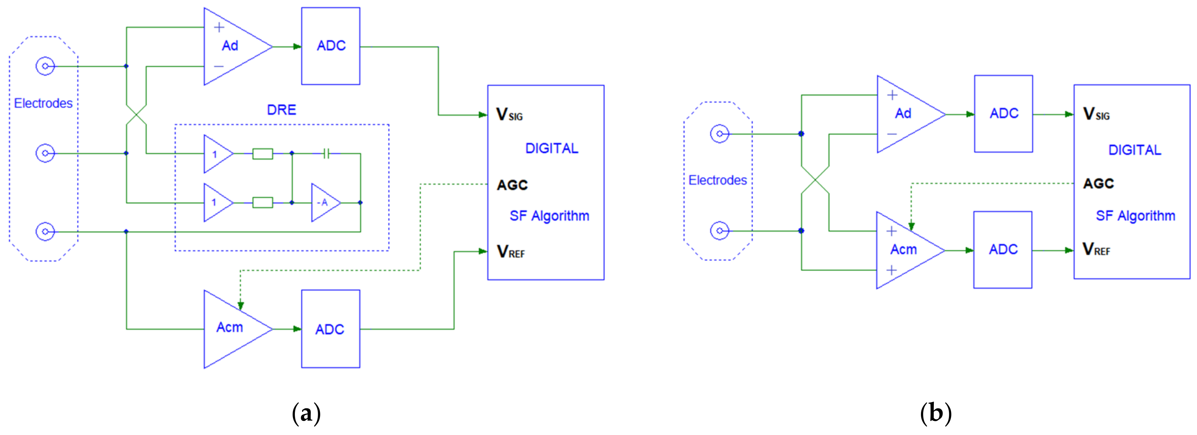
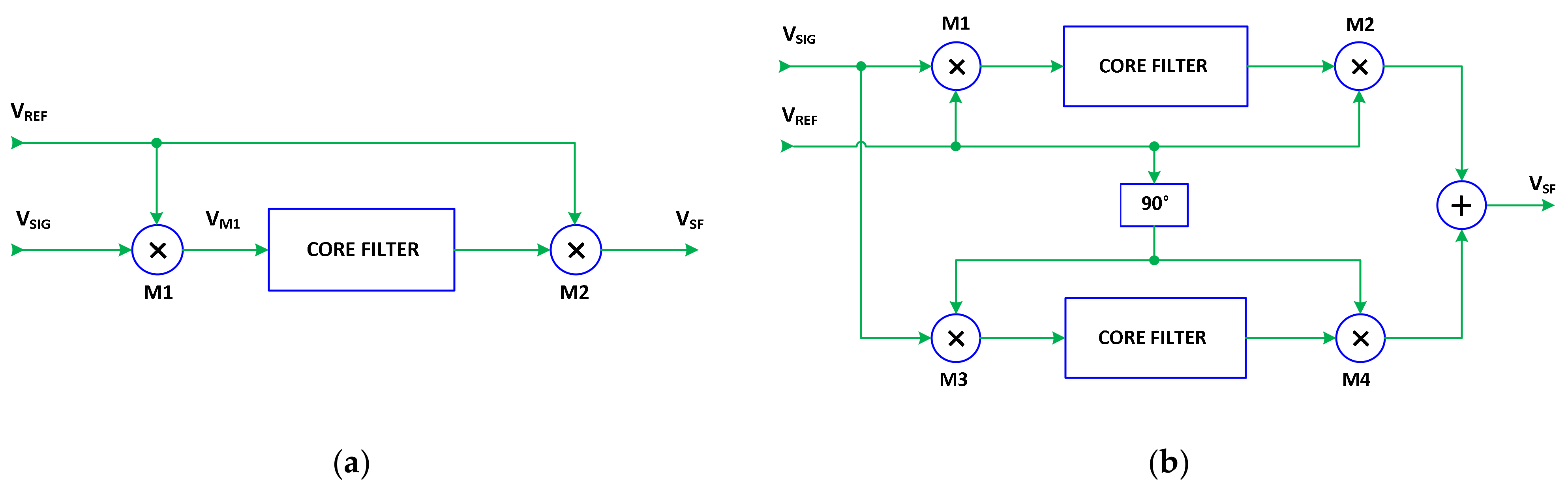
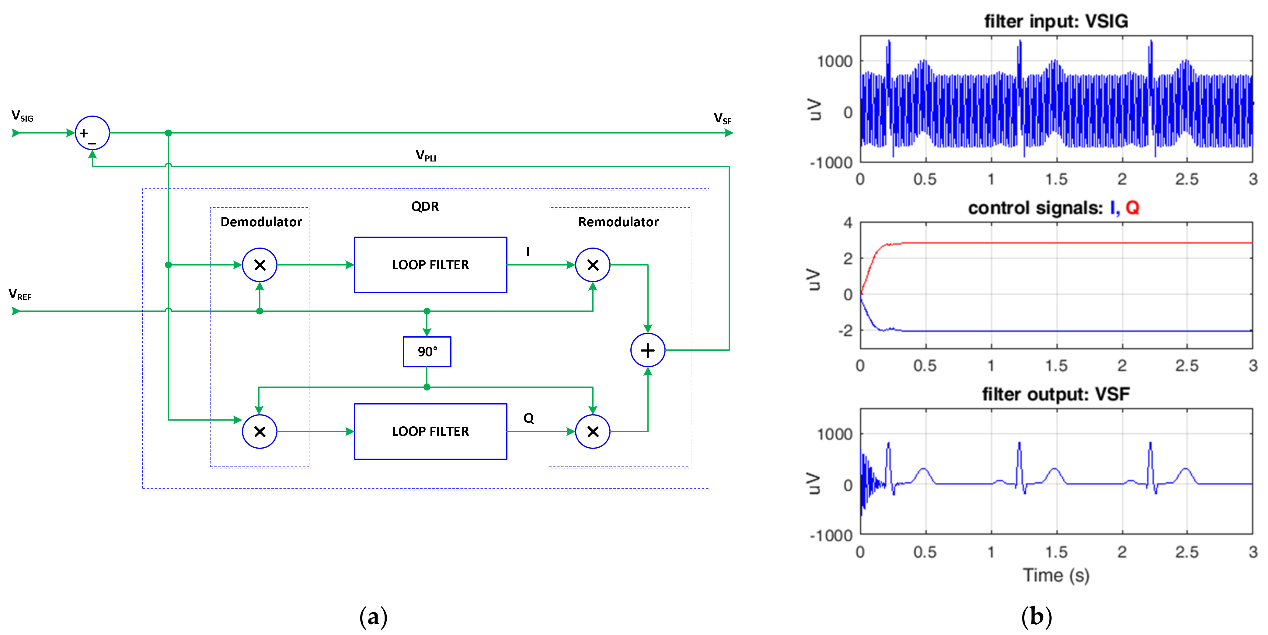
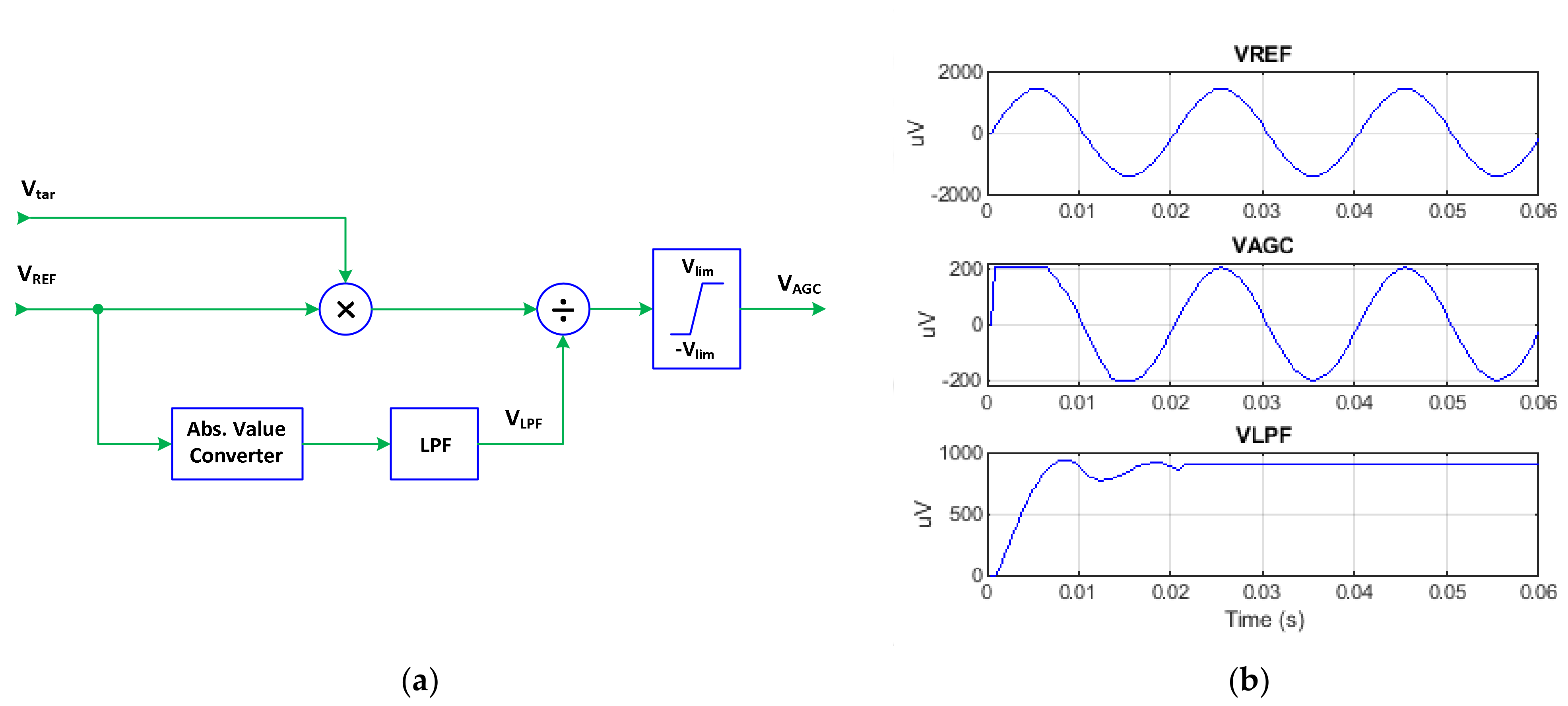
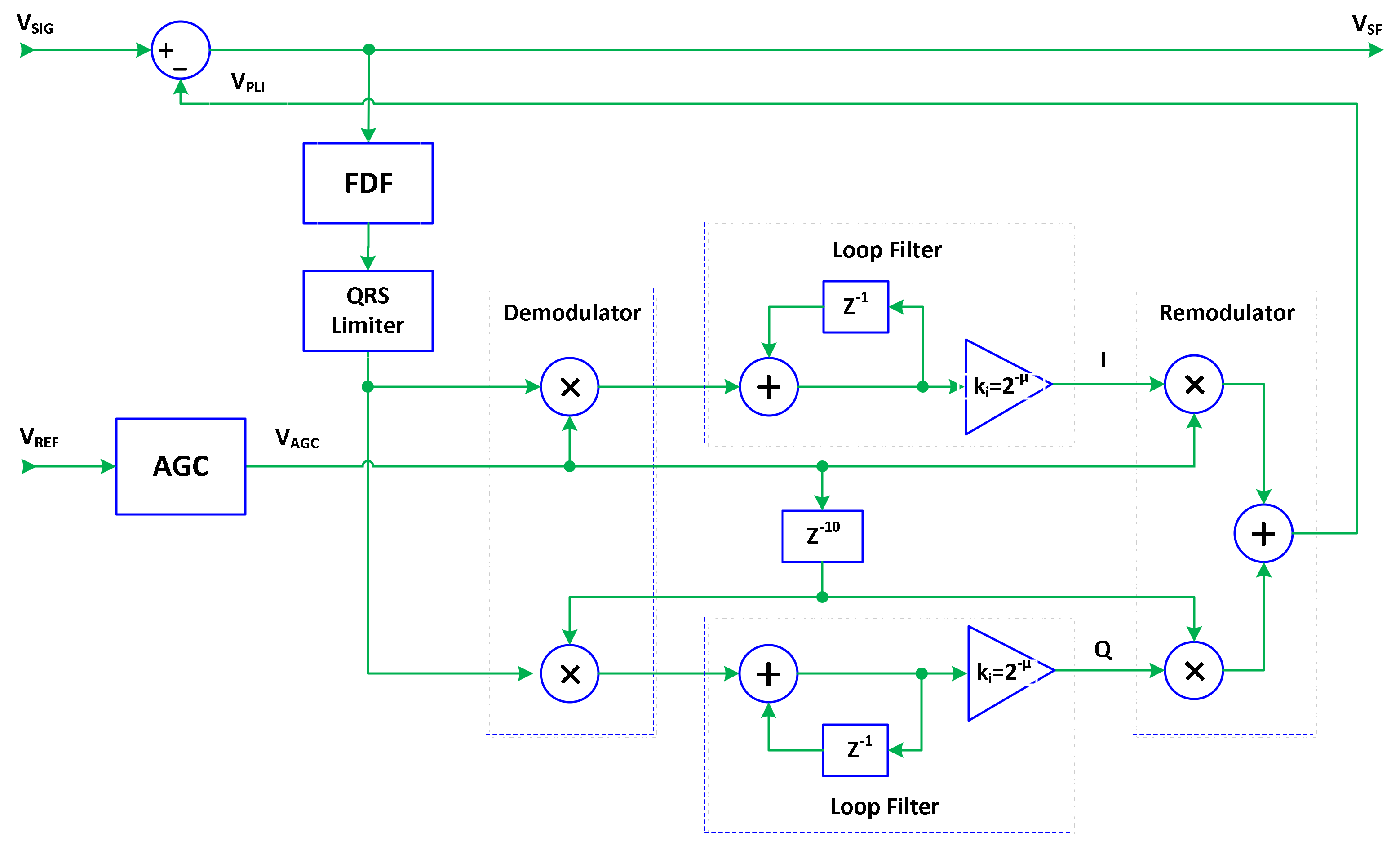
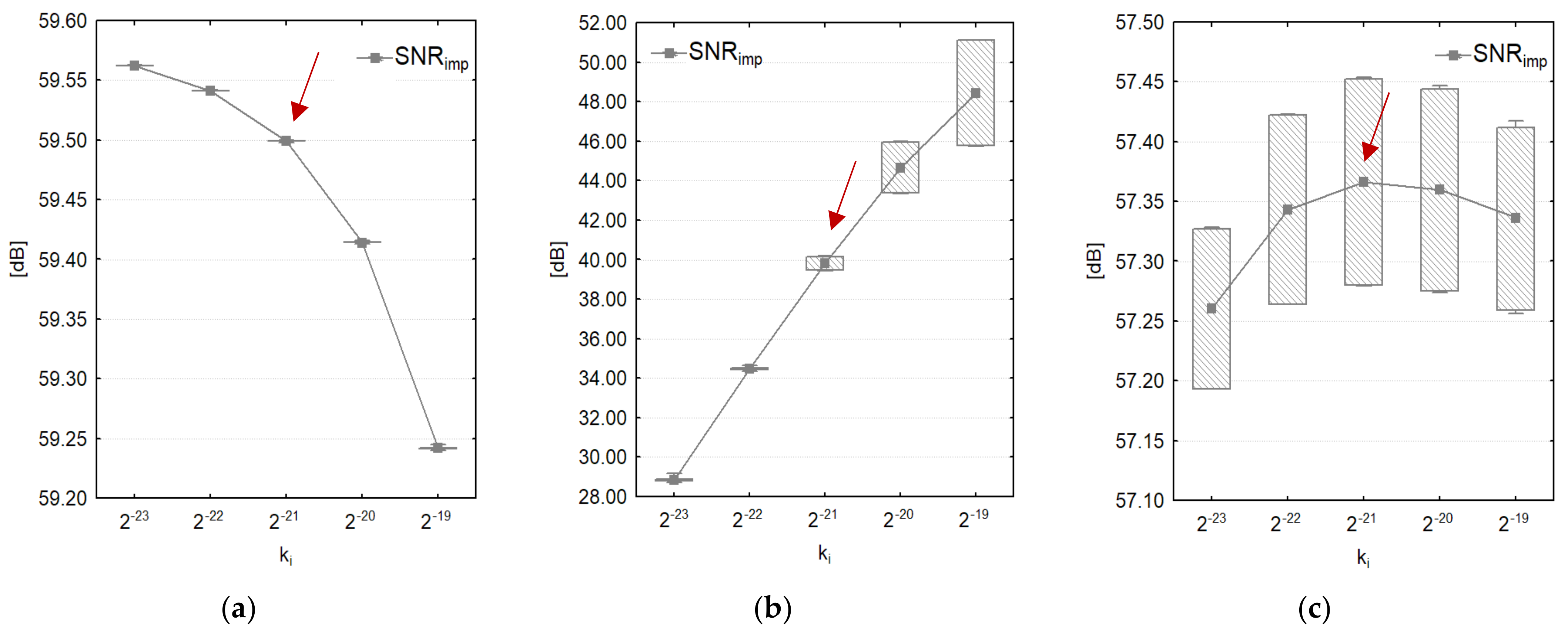
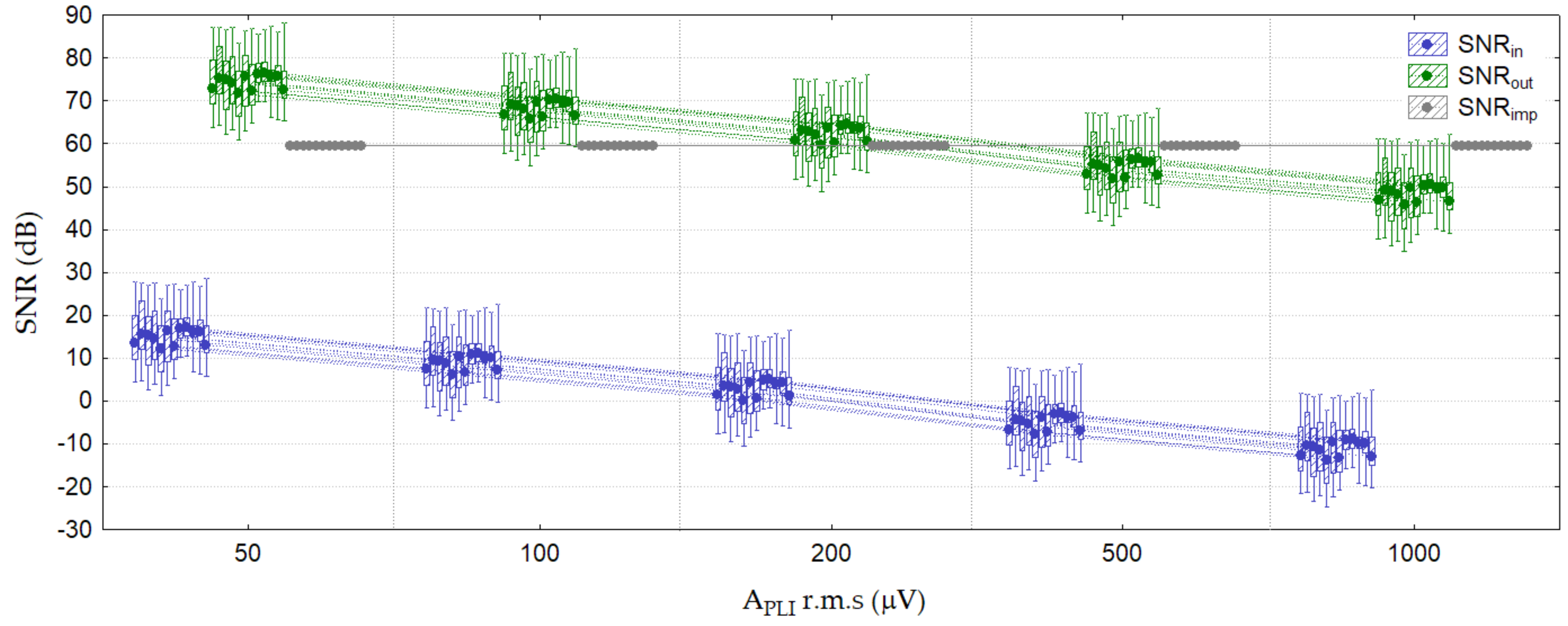
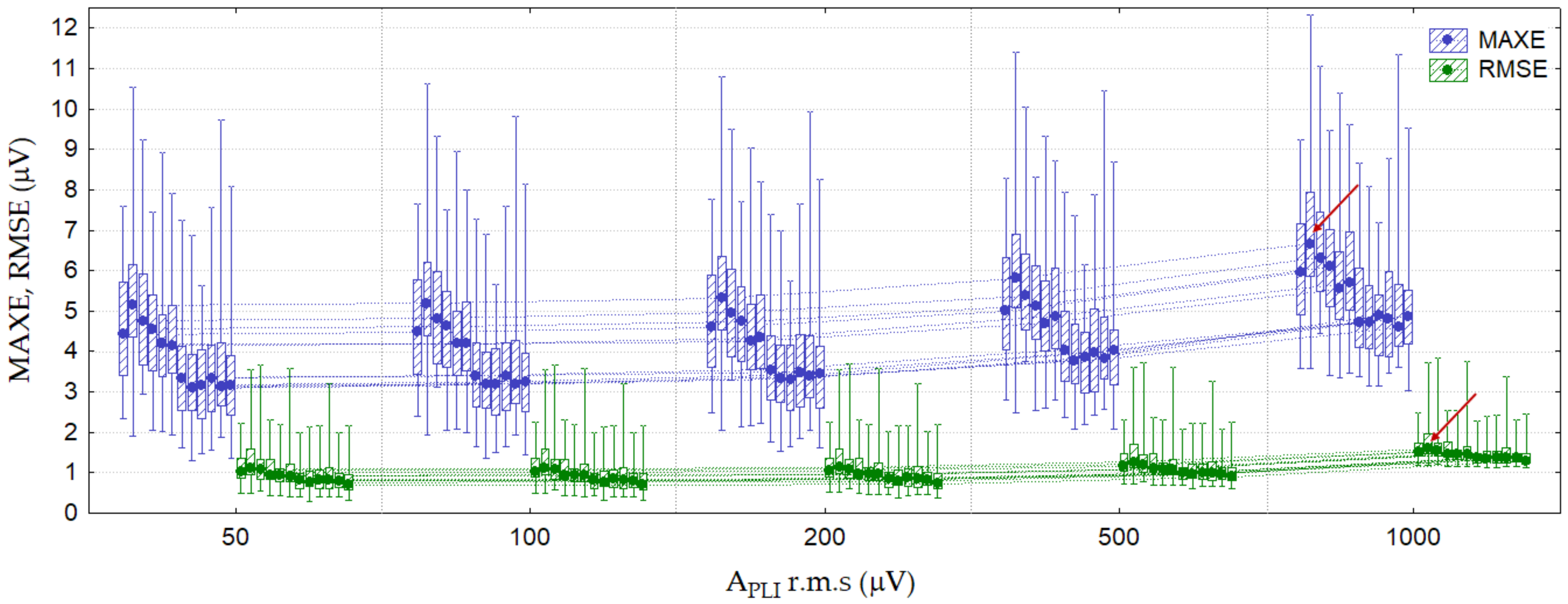
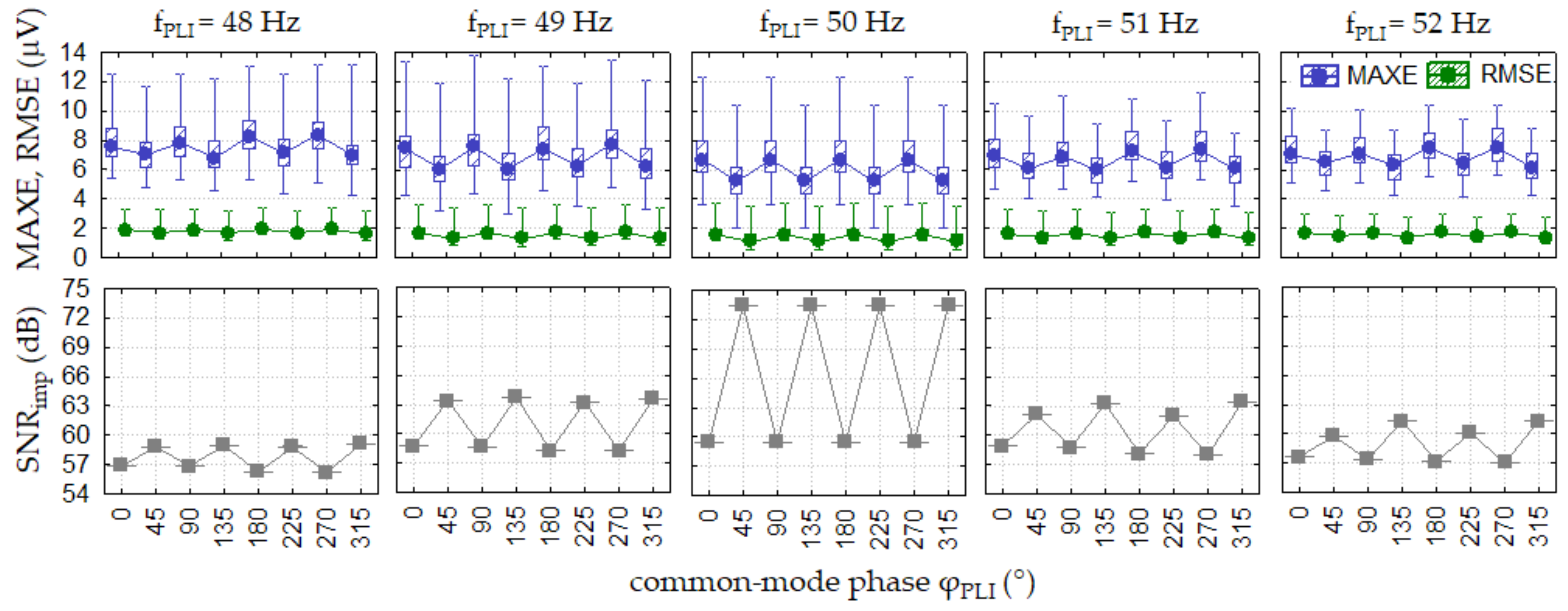
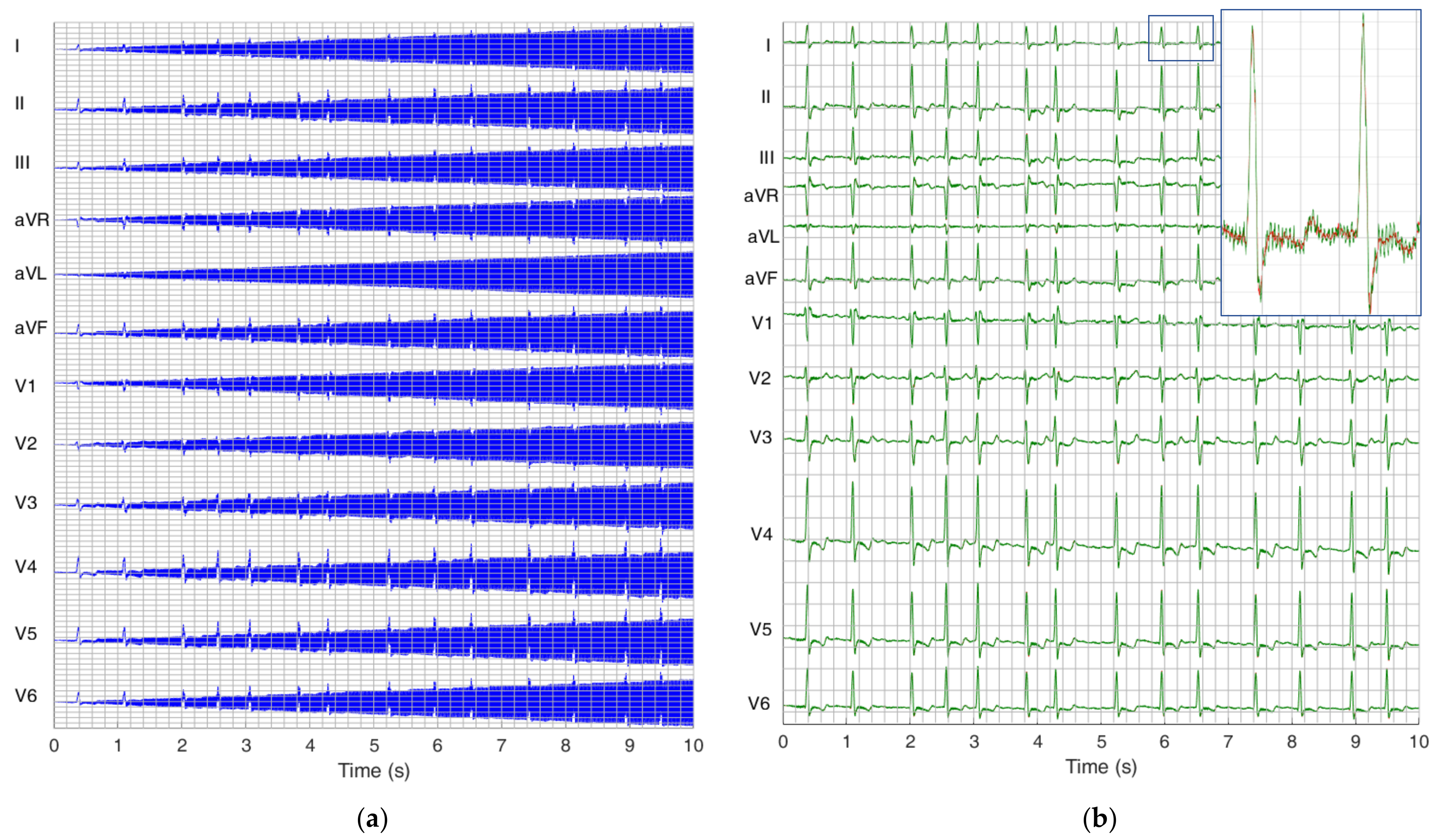
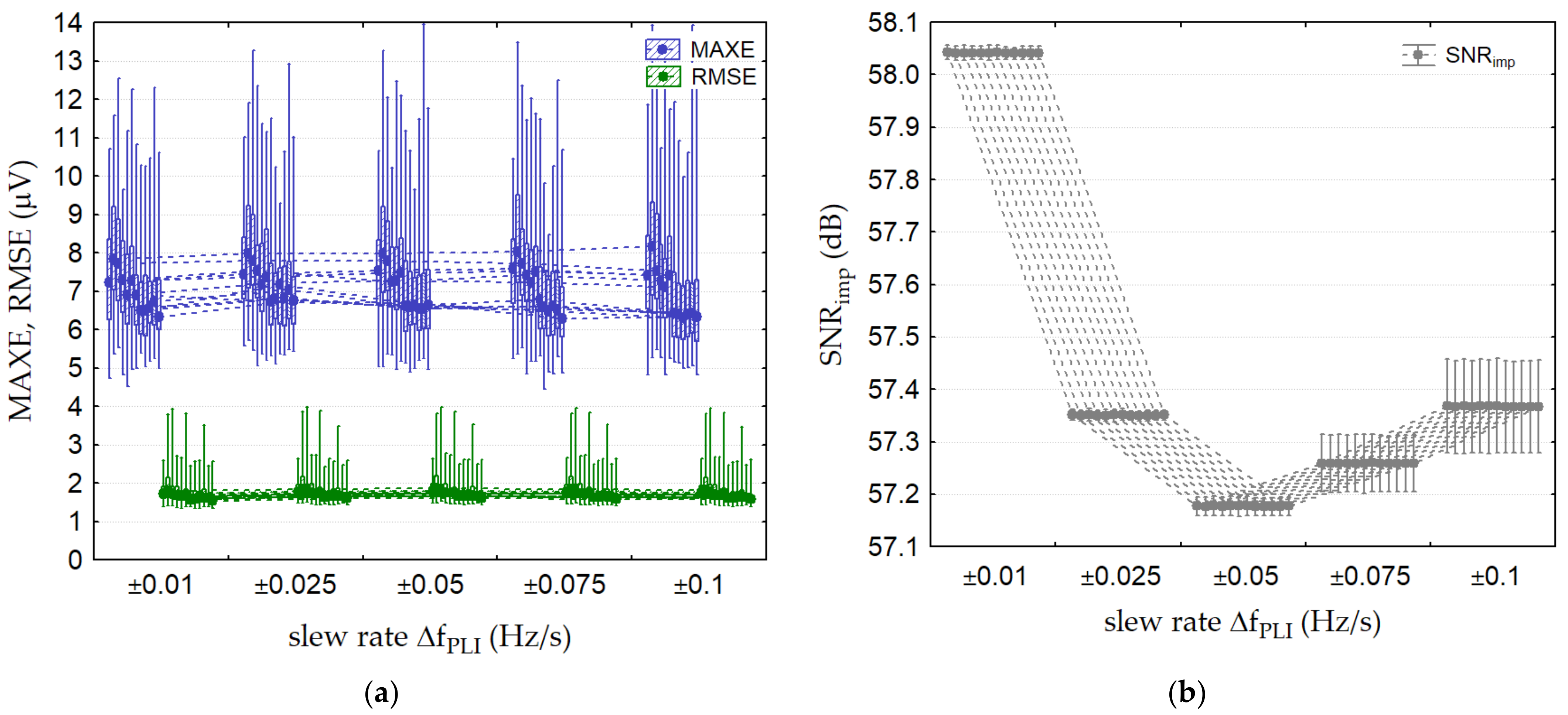
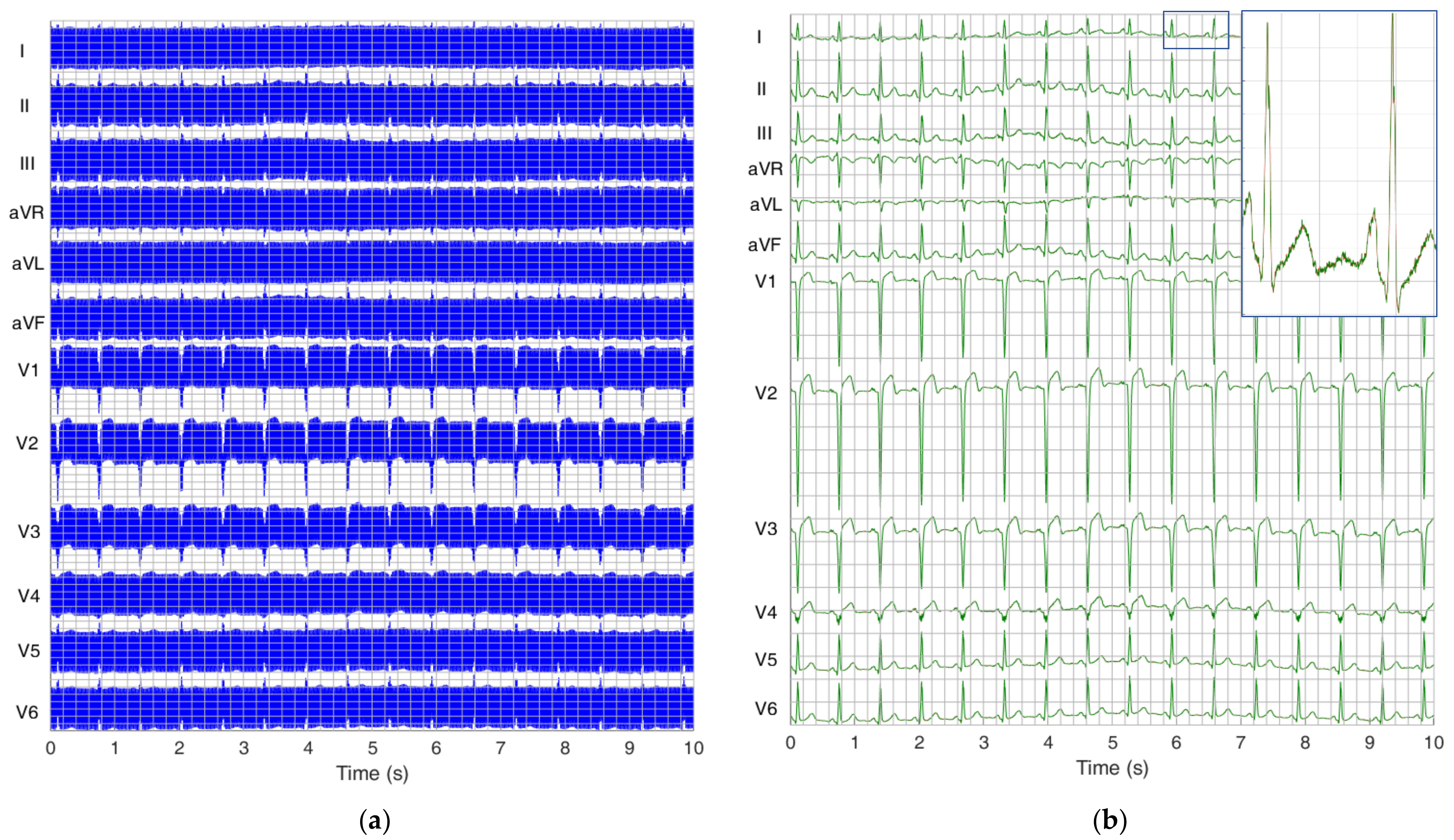
Table 1.
Simulation parameters of PLI with duration of 10 s for 3 optimization scenarios with CTS-ECG calibration database.
Table 1.
Simulation parameters of PLI with duration of 10 s for 3 optimization scenarios with CTS-ECG calibration database.
| PLI Amplitude APLI r.m.s (μV) | PLI Amplitude Slew Rate ΔAPLI (μV/s) | PLI Frequency Range fPLI (Hz) | PLI Frequency Slew Rate ΔfPLI (Hz/s) | |
|---|---|---|---|---|
| PLI constant | 1000 | 0 | 50 | 0 |
| PLI linear amplitude change | 1000 | ±200 | 50 | 0 |
| PLI linear frequency change | 1000 | 0 | 49–51 | ±0.1 |
Table 2.
Simulation parameters of PLI with duration of 10 s for five test scenarios with PTB Diagnostic ECG database.
Table 2.
Simulation parameters of PLI with duration of 10 s for five test scenarios with PTB Diagnostic ECG database.
| PLI Ampl. APLI r.m.s (μV) | PLI Ampl. Slew Rate ΔAPLI (μV/s) | PLI Frequency fPLI (Hz) | PLI Frequency Slew Rate ΔfPLI (Hz/s) | VREF Phase φPLI (°) | ECG Leads | |
|---|---|---|---|---|---|---|
| Test 1: PLI constant (amplitude test) | 50, 100, 200, 500, 1000 | 0 | 50 | 0 | 0 | 12 leads |
| Test 2: PLI constant (frequency test) | 1000 | 0 | (48, 48.1, 48.2, …, 51.8, 51.9, 52) | 0 | 0 | worst lead in Test 1 |
| Test 3: PLI constant (common-mode phase test) | 1000 | 0 | (48, 49, 50, 51, 52) | 0 | (0, 45, 90, 135, 180, 225, 270, 315) | worst lead in Test 1 |
| Test 4: PLI linear amplitude change | (50, 100, 200, 500, 1000) | ±(10, 20, 40, 100, 200) | 50 | 0 | 0 | 12 leads |
| Test 5: PLI linear frequency change | 1000 | 0 | 50 | ±(0.01, 0.025, 0.05, 0.075, 0.1) | 0 | 12 leads |
Table 3.
Extremity PLI parameters for which SF algorithm fulfils the standard for powerline filers in diagnostic electrocardiographs [41]. Maximal SF errors are reported as median value (min–max range) found in lead II (PTB Diagnostic ECG database) and V2 (CTS-ECG analytical database), where denoted with *.
| PTB Diagnostic ECG Database 12 Leads | CTS-ECG Analytical Database 8 Leads | ||||||
|---|---|---|---|---|---|---|---|
| Setting with Maximal Error | MAXE (μV) | RMSE (μV) | SNRimp (dB) | MAXE (μV) | RMSE (μV) | SNRimp (dB) | |
| Test 1: PLI constant (amplitude test) | Lead II, V2 * APLI = 1000 μV r.m.s. fPLI = 50 Hz | 6.7 (3.5–12.5) | 1.5 (1.2–2.8) | (60) | 2.4 (2.3–5.5) | 1.1 (1.1–1.7) | (60) |
| Test 2: PLI constant (frequency test) | Lead II, V2 * APLI = 1000 μV r.m.s. fPLI = 49.3–49.9 Hz | 8.5 (5–15) | 2 (1.2–3.8) | (57–58) | 6.4 (4–8.2) | 1.5 (1.4–2.1) | (57–58) |
| Test 3: PLI constant (common-mode phase test) | Lead II, V2 * APLI = 1000 μV r.m.s. fPLI = 48, 52 Hz | 8 (2.5–14) | 2 (1.8–3.8) | (57–62) | 5 (2.5–8.1) | 1.6 (0.7–2.8) | (57–62) |
| Test 4: PLI linear amplitude change | Lead V2 ΔAPLI = ±40 μV/s fPLI = 50 Hz | 12 (7–17) | 4 (2–7) | (39.8) | 13 (11–14.5) | 5 (2.8–6) | (39.8) |
| Test 5: PLI linear frequency change | Lead II, V2 * APLI = ±1000 μV r.m.s. ΔfPLI = 0.1 Hz/s | 8.2 (5–14) | 1.8 (1.5–4) | (57.3) | 6.5 (4.1–19.8) | 1.5 (1.2–4.2) | (57.3) |
Table 4.
Comparative study with other published papers on PLI filtering in ECG found to provide a comprehensive numerical evaluation of the filer outputs by at least one of the performance metrics calculated in this study. The performances are listed as reported in original articles, representing mean values if several records from a test database were evaluated, otherwise representing a single measurement from one ECG signal.
| Study | Database | Methods | PLI Freq [Hz] | SNRin (dB) | SNRout (dB) | SNRimp (dB) | MAXE (μV) | RMSE (μV) |
|---|---|---|---|---|---|---|---|---|
| This study | DB1 | • Common-mode Driven Synchronous Filtering | 50 | −10–15 | 50–75 | 60 | 3–6.7 | 0.8–1.5 |
| 48 | −5 | 52 | 57 | 7.6 | 1.9 | |||
| 52 | −5 | 53 | 58 | 7.0 | 1.8 | |||
| 50 | −10–15 # | 30–55 | 40 | 1–14 | 5–42 | |||
| 49–51 # | −5 | 52 | 57 | 6.8 | 1.8–2 | |||
| Chaitanya and Sharma (2022) [53] | DB2 | • Four-stage cascaded Savitzky–Golay filter | 50 | −5 | 20.3 | 25.3 | NA | 9.6 |
| 50 | −10 | 16.8 | 26.8 | NA | 14.4 | |||
| Tanji et al. (2021) [12] | 1 ECG record | • Moving average PLL | 60 | −11.6 | 38.9 | 50.6 | 300 | NA |
| 66.7 | −11.6 | 46.9 | 58.5 | 300 | NA | |||
| 50.9 | −11.6 | 30.6 | 42.2 | 500 | NA | |||
| Martens et al. (2006) [54] | 1 ECG record | • Improved adaptive filter | 50 | −20–20 | 36 | 16–56 | NA | NA |
| • Simple adaptive filter | 50 | −20–20 | 19–24 | 4–49 | NA | NA | ||
| • Wide notch filter | 50 | −20–20 | 15 | 5–35 | NA | NA | ||
| • Narrow notch filter | 50 | −20–20 | 23 | 3–53 | NA | NA | ||
| • Improved adaptive filter | 48–52 # | 0 | 37 | 37 | NA | NA | ||
| • Simple adaptive filter | 48–52 # | 0 | 20 | 20 | NA | NA | ||
| • Wide notch filter | 48–52 # | 0 | 15 | 15 | NA | NA | ||
| • Narrow notch filter | 48–52 # | 0 | 11 | 11 | NA | NA | ||
| Rahman et al. (2013) [28] | DB2 | • Leaky block adaptive filter | 50 | NA | NA | 11–31 | NA | NA |
| Razzaq et al. (2016) [55] | 1 ECG record | • State space RLS adaptive filter | 50.38 | 1.4–7.5 | 25–32 | 24 | NA | NA |
| 50.38 | 2.5 # | 28 | 26 | NA | NA | |||
| 50.4–51.8 | 7.5 | 22 | 15 | NA | NA | |||
| Saxena et al. (2019) [56] | DB2 | • Normalized LMS adaptive filter | 50 | NA | 51 | NA | NA | 1.5 |
| • Discrete wavelet transform | 50 | NA | 36 | NA | NA | 8.6 | ||
| • IIR filter (order 8) | 50 | NA | 28 | NA | NA | 19.5 | ||
| • FIR filter (order 50) | 50 | NA | 26 | NA | NA | 25.8 | ||
| Tomasini et al. (2016) [57] | DB1 | • RLS adaptive filter | 50–51 | −20–20 | 35 | 15–55 | NA | NA |
| Verma and Singh (2015) [17] | 1 ECG record | • Adaptive notch FIR filter with tunable notch frequency | 50 | 7–15 | 14–25 | 7–10 | NA | NA |
| Biswas and Maniruzzaman (2014) [58] | DB2 | • Normalized LMS adaptive filter | 50 | NA | 6.3 | NA | NA | 5.6 |
| • RLS adaptive filter | 50 | NA | 6.7 | NA | NA | 8.9 | ||
| • Notch filter | 50 | NA | 6.7 | NA | NA | 7.9 | ||
| Satija et al. (2017) [59] | DB2 | • Notch filter | 50 | NA | 30.1 | NA | 100 | NA |
| • LMS adaptive filter | 50 | NA | 25.3 | NA | 130 | NA | ||
| • Algorithm using ECG noise-aware dictionary, sparse signal decomposition, and reconstruction | 50 | NA | 32.9 | NA | 50 | NA | ||
| Kumar et al. (2020) [60] | DB1, DB2, DB3 | • Synchrosqueezing transform with adaptive filter | 50 | −3 | NA | 48–52 | NA | 8.2–13 |
| 48 | −3 | NA | 47–49 | NA | 3.6–15 | |||
| 52 | −3 | NA | 49–50 | NA | 3.4–12 | |||
| Bodile and Talari (2021) [61] | DB2 | • Discrete wavelet transform | 50 | −10–10 | 6–23 | 13–16 | NA | NA |
| • Empirical mode decomposition | 50 | −10–10 | 20–23 | 23–30 | NA | NA | ||
| • Kalman filter | 50 | −10–10 | 22–23 | 13–22 | NA | NA | ||
| • Kalman backward–forward filter | 50 | −10–10 | 22–23 | 13–33 | NA | NA | ||
| Zhou and Zhang (2013) [9] | DB1 | • Hybrid filter with two-sided filtration and multi-iterative approximation techniques | 50 | 10 | 25.4 | 15.4 | NA | NA |
| Leski (2021) [62] | DB1 | • Nonlinear aggregation operator | 50 | (−5; 0) * | NA | NA | 1.3–35.5 | 1–17.4 |
| Mateo et al. (2008) [63] | DB1, DB2, DB3 | • Notch filter | 48.5–51.5 | NA | NA | 14 | NA | 3.5–42 |
| • Notch adaptive filter | 48.5–51.5 | NA | NA | 15 | NA | 2.1–32 | ||
| • Artificial neural network | 48.5–51.5 | NA | NA | 19 | NA | 1.5–16 | ||
| Qui et al. (2017) [64] | DB2 | • Recurrent neural network | 50 ± 0.1 | 0 | 36 | 36 | NA | NA |
| • Kalman smoother | 50 ± 0.1 | 0 | 32 | 32 | NA | NA | ||
| • IIR notch filter | 50 ± 0.1 | 0 | 23 | 23 | NA | NA | ||
| Poungponsri and Yu (2013) [65] | DB2 | • Wavelet transform and artificial neural network | 60 | 11 | 33 | 22 | NA | NA |
| Chatterjee et al. (2022) [66] | DB2 | • Sparsity-based wavelet denoising neural network autoencoder | 50 | 5 | 27.4 | 22.4 | NA | 16.8 |
LMS: least mean square; RLS: recursive least square; IIR: infinite impulse response; FIR: finite impulse response; PLL: phase-locked loop; NA: no available data in the original paper. DB1: PTB diagnostic database; DB2: MIT-BIH arrhythmia database; DB3: St. Petersburg 12-lead arrhythmia database. # PLI with linearly changing amplitude or frequency. * Results in [62] are reported for peak-to-peak PLI amplitude of 500 µV, corresponding to SNR in range of −5 to 0 dB, according to Figure 9 (PLI amplitude range between 200 and 500 µV r.m.s. estimated with samples from the same ECG database (DB1)).
Publisher’s Note: MDPI stays neutral with regard to jurisdictional claims in published maps and institutional affiliations. |
© 2022 by the authors. Licensee MDPI, Basel, Switzerland. This article is an open access article distributed under the terms and conditions of the Creative Commons Attribution (CC BY) license (https://creativecommons.org/licenses/by/4.0/).
Share and Cite
MDPI and ACS Style
Neycheva, T.; Dobrev, D.; Krasteva, V. Common-Mode Driven Synchronous Filtering of the Powerline Interference in ECG. Appl. Sci. 2022, 12, 11328. https://doi.org/10.3390/app122211328
AMA Style
Neycheva T, Dobrev D, Krasteva V. Common-Mode Driven Synchronous Filtering of the Powerline Interference in ECG. Applied Sciences. 2022; 12(22):11328. https://doi.org/10.3390/app122211328
Chicago/Turabian StyleNeycheva, Tatyana, Dobromir Dobrev, and Vessela Krasteva. 2022. "Common-Mode Driven Synchronous Filtering of the Powerline Interference in ECG" Applied Sciences 12, no. 22: 11328. https://doi.org/10.3390/app122211328
Note that from the first issue of 2016, this journal uses article numbers instead of page numbers. See further details here.