
Estimation and Reliability Research of Post-Earthquake Traffic Travel Time Distribution Based on Floating Car Data
College of Transportation Engineering, Nanjing Tech University, Nanjing 211816, China
*
Authors to whom correspondence should be addressed.
Appl. Sci. 2022, 12(18), 9129; https://doi.org/10.3390/app12189129
Submission received: 17 July 2022
/
Revised: 6 September 2022
/
Accepted: 7 September 2022
/
Published: 11 September 2022
(This article belongs to the Special Issue Seismic Performance Assessment for Structures)
Abstract
:To carry out the estimation and reliability research of post-earthquake traffic travel time, which has the great influence for efficient allocation of relief materials. By analyzing the relationship among floating vehicle trajectory, target path and road network path, the intermediate parameters of converting floating vehicle trajectory data into target path travel time were defined and improved. In addition, the road damage identification method relying on lane detection is applied for evaluating the damage of road after the earthquake through the image information. Then, Bayesian average adaptive kernel density estimation method was used to estimate the distribution of post-earthquake road travel time, and a new formula for calculating the reliability of road travel time after earthquake was proposed. According to the example simulation and analysis, the proposed post-earthquake road travel time distribution estimation and its reliability are verified. The results show that when the threshold value is determined, the travel time of the path before the earthquake is the most dependable, and with the increase in the earthquake damage index, the travel time of this road section becomes increasingly unreliable. However, after the earthquake, the peak probability density of road travel time distribution weakens, and the overall probability shifts to the direction of long time.
1. Introduction
Over the past decades, natural disasters such as floods, tornadoes, earthquakes, volcanic eruptions, and tsunami have caused human society huge property losses and casualties. In the case of an earthquake, once it occurs, in addition to causing surface rupture, it will also produce a series of continuous events such as landslides, landslides, and building collapse, all these impacts will cause serious damage to the highway system [1], seriously affecting the transport of relief supplies and the transfer of casualties, so the reconstruction and optimization of the post-disaster traffic network [2] is very important. With the development of floating car detection technology [3,4], this key issue has become technically feasible, and people have begun to study how to provide travelers with more accurate travel time information, so that they can make wise route selection plans [5]. At the same time, it has become one of the important research directions of disaster prevention and mitigation engineering to analyze the road damage after earthquake and predict the connectivity of traffic network with floating vehicle technology.
Recently, floating car technology has been developed rapidly, focusing on traffic data extraction technology, traffic state estimation, traffic events (traffic congestion) identification. J.L. Ygnace et al. [6] had tested network-based cellular location methods for assessing emergency call management on national roads and highways while estimating travel times on sections of roads on account of vehicles currently equipped with mobile phones. While Wang li et al. [7] studied the calculation method of floating vehicle sample size, improved the calculation model of J.L. Ygnace trade’s floating vehicle sample size, and established the basic theoretical framework for collecting traffic data by floating vehicle method. Schafer et al. [8] proposed a system framework for floating car traffic data extraction, which could realize travel time prediction and optimal route selection by taking taxi as floating car data acquisition carrier. Kerner [9] used high-quality floating car travel time data to detect traffic events on the urban road network. With the rapid development of data processing technology, a new type of extended floating car technology was taken into application, which means more sensors for the floating car. Image recognition equipment, which can identify the road information of the floating car, was widely used because its recognition of signal lights. Messelodi [10] combined intelligent vehicle and floating vehicle technologies and purposed a road condition recognition system derived from image recognition, including the recognition of road signs and pavement.
At present, the research level of travel time calculation gained from floating car data has been improved. According to the travel rules of travelers, Zhang Jian et al. [11] divided the paths into the shortest path, the fastest path, and the preferred path, and suggested three preferred origin destination (OD) travel time prediction methods, believing that this method can significantly improve the prediction accuracy of OD travel time. To solve the problem of real-time floating car data sparse, Zhang Fangli et al. [12] used multi-layer neural network to conduct reinforcement learning on the relationship between feature and travel time of target road section and adjacent road section and obtained the predicted travel time of target road section. The results showed this method can also be used to solve the problem of partial missing of offline data. Zheng Yeqing et al. [13] designed a travel time estimation model gained from road network similarity, which is derived from road attributes such as road length, road analysis, number of lanes, and similarity characteristics such as access degree of each road section and point of interest (POI) intensity. From the perspective of road network similarity, the feasibility of solving real-time data missing is verified. Yilun Wang et al. [14] created a real-time city-wide model to estimate the travel time of any route in the city. Modeling the driving time of different drivers in different sections shows the effectiveness of the method. A deep learn-based travel time estimation model that neighbors for travel time estimation (Nei-TTE) was used for the first time by Qiu Jing et al. [15]. It can effectively simulate the topological information of the surrounding space by using the velocity characteristics and assign an exact start time to each section. Experiments on large-scale real data sets show that the proposed method achieves better estimation results and is obviously superior to existing models. Erik Jenelius et al. [16] proposed a statistical model to estimate the travel time of the urban road network by taking the vehicle track acquired by low-frequency global position system (GPS) probe as the observation value and dividing the model travel time into road segment travel time and intersection delay time. Based on the Spatial Moving Average (SMA) structure, the correlation between travel time on different network links is allowed. Then, the model was applied to the Stockholm network in Sweden. The results showed that road attributes and travel conditions (including recent snowfall) had a significant impact on travel time. There is a significant positive correlation between each stage. Ma et al. [17] studied a generalized Markov chain method, which weighted the travel time distribution of Markov paths according to its probability of occurrence to obtain the probability distribution of travel time. The link travel time distribution depends on current link traffic and can be estimated from historical observations. The algorithm, based on moment generation function, is used to approximate the sum of the travel time distributions of related links to the travel time distributions of Markov paths under traffic conditions. The method is applied to examine a traffic case study using automatic vehicle location data. Shi et al. [18] considered a robust travel time distribution estimation method, using emerging low-frequency floating car data to estimate the mean and variance of travel time, and designed a distribution estimation algorithm to estimate random turn delay. A case study of Wuhan, China, was taken to verify the applicability of this method.
The research of post-earthquake transportation systems abroad in wide-ranging, including post-earthquake road emergency repair, post-earthquake road network reliability and vulnerability analysis, and post-earthquake recovery process. Contreras et al. [19] believed that spatial connectivity is an effective spatial index for monitoring and evaluating the post-earthquake recovery process, which integrates the variables of distance, travel time, and quality of public transport service after assuming the relationship between the connectivity of the urban center and the location of the new resettlement sites assigned to the homeless during the recovery process. Khademi et al. [20] found out the areas along with the quake route which were most likely to be disrupted by earthquakes. Akbari et al. [21] studied the planning of post-earthquake emergency repair, especially the re-opening of damaged roads, and produced an accurate algorithm of mixed integer programming (MIP). By clustering trips with the same starting point in a specific time interval, Fang et al. [22] developed a temporal graph neural network with heterogeneous features (TGCNHF) with heterogeneous characteristics, thereby introducing network trip risk (NTR) to evaluate the reliability of this region.
There were relatively few studies on the reliability of post-earthquake travel time. Zhang et al. [23] creatively extracted spatial-temporal traffic features by using gray level co-occurrence matrix (GLCM) and introduced them into the pattern matching method of travel time. Different from previous methods, this method used large-scale spatial-temporal traffic patterns to predict multi-step travel time. Shen Xiaobing et al. [24] constructed the graphic evaluation, reviewed technique (GERT) reliability model for the arrival time of emergency rescue and proposed the GERTS simulation algorithm based on the analysis of post-earthquake roadblock risk probability, travel time fluctuation and path choice preference. Hou Benwei et al. [25] studied the reliability of traffic travel time after an earthquake, used Monte Carlo simulation method to simulate the connectivity of road network after an earthquake. This method could predict the reliability of traffic travel time after an earthquake on this basis, emphasized the impact of building collapse on the reliability of road travel time. Zhang Yuhong et al. [26] constructed a weighted network model of urban bus based on Space L method considering trip time reliability and took network connectivity rate and network trip time reliability as metrics to study the survivability of urban bus network. Xue Xiaojiao et al. [27] analyzed the relationship among path, OD pair, road network trip and road network trip time reliability under emergency conditions and established a VISSIM simulation model. The results showed that with the decrease in emergency events, road network trip time reliability would also decline.
Until now, the research on floating vehicle data processing and probability distribution estimation of travel time under normal traffic remains immature, the research on post-earthquake emergency rescue stage is still basically blank. Hence, combining the estimation method of the probability distribution of travel time with the existing research results of earthquake road vulnerability, and gives the estimation method of the probability distribution of post-earthquake travel time, which is great significance to improve the ability of disaster prevention and mitigation of transportation system. This research gives an index to quantify the reliability of road travel time, namely degree of travel time reliability. In combination with road earthquake damage factors, the authors use Bayesian Adaptive Kernel Density Estimation method to improve the weighting coefficient of the probability density function of road travel time after an earthquake. To obtain a formula for calculating degree of travel time reliability which can be used for relevant departments to judge the reliability of road networks, this paper also provides effective basis for improving the speed of material transportation and emergency rescue.
2. Data Processing and Track Information Extraction of Floating Vehicle
2.1. Floating Car Data Characteristics and Preprocessing
The floating car data used in this paper are mainly longitude, latitude and time, and its data format and examples are as follows:
Taxi ID, latitude, longitude, passenger carrying state, time point, [speed];
1, 30.4996330000,103.9771760000,1,2014/08/03 06:01:22, [65.1];
1, 30.4936580000,104.0036220000,1,2014/08/03 06:02:22, [64.8];
2, 30.6319760000,104.0384040000,0,2014/08/03 06:01:13, [66.5].
The data uploaded by emergency rescue vehicles after the earthquake is also a form of floating vehicle data. Therefore, it is necessary to study the information extraction method from the data characteristics and error analysis of general floating vehicles.
(1) Data cleaning
In view of the small amount of data from 00:00:00 to 05:59:59 at night, and the travel time prediction in this period is of no practical significance, this paper excluded the data in this period. If the same vehicle stays for more than 5 min, the recorded data will also be removed. In addition, obvious outliers caused by data transmission need to be eliminated, such as missing part of data or records of longitude and latitude deviating too far from the road section.
(2) Data filling
Using fuzzy C- means (FCM) algorithm to fill the missing data of floating car [28]. At the same time, the FCM clustering as Algorithm 1, the filling process is summarized in the following steps:
| Algorithm 1. FCM algorithm. |
| Begin Setting template function precision ε, fuzzy index m and maximum iteration number Tm. Initializing a fuzzy clustering center zi. Repeat Update the fuzzy partition matrix U = {μij} and the cluster center z = {ZC}. t ← t + 1 Until (|J(t) − J(t − 1)| < ε OR c > Tm) The result of pixel classification is obtained from the obtained U = {μij}. Make use of cluster center zi to fill the vacancy. End |
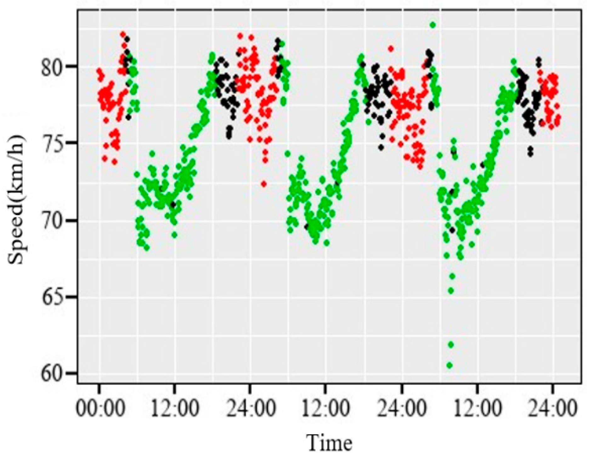
The clustering results of floating car data collected from The Second Ring Road of Chengdu from 3 August to 5 August 2014, based on FCM clustering algorithm, are shown in Figure 1. Table 1 shows the velocity values of different clustering centers obtained according to FCM clustering algorithm; the missing data can be directly replaced by the cluster center value in the table. According to the results in these, vehicle speeds are concentrated in the range of 67.5~82.5, and the speed center value of different clusters is around 75.
2.2. Definition of Basic Parameters of Floating Car Method
(1) The coverage of the target path to the road
Section path is defined as an acyclic directed path π = (ks, k′, …, k′′, ke), and os is defined as the distance from the starting point of the road section ks to the starting point of the route; oe is the distance from the start of the section ke to the end of the route. For a road section k, if the length covered by the path π on the road section k is ak, then:
According to Formula (1) [29], the coverage degree αk of the route to the road section k can be calculated by comparing the covered length ak with the total length lk of this road section, and the calculation formula is αk = ak/lk.
(2) The coverage of the floating car track road section
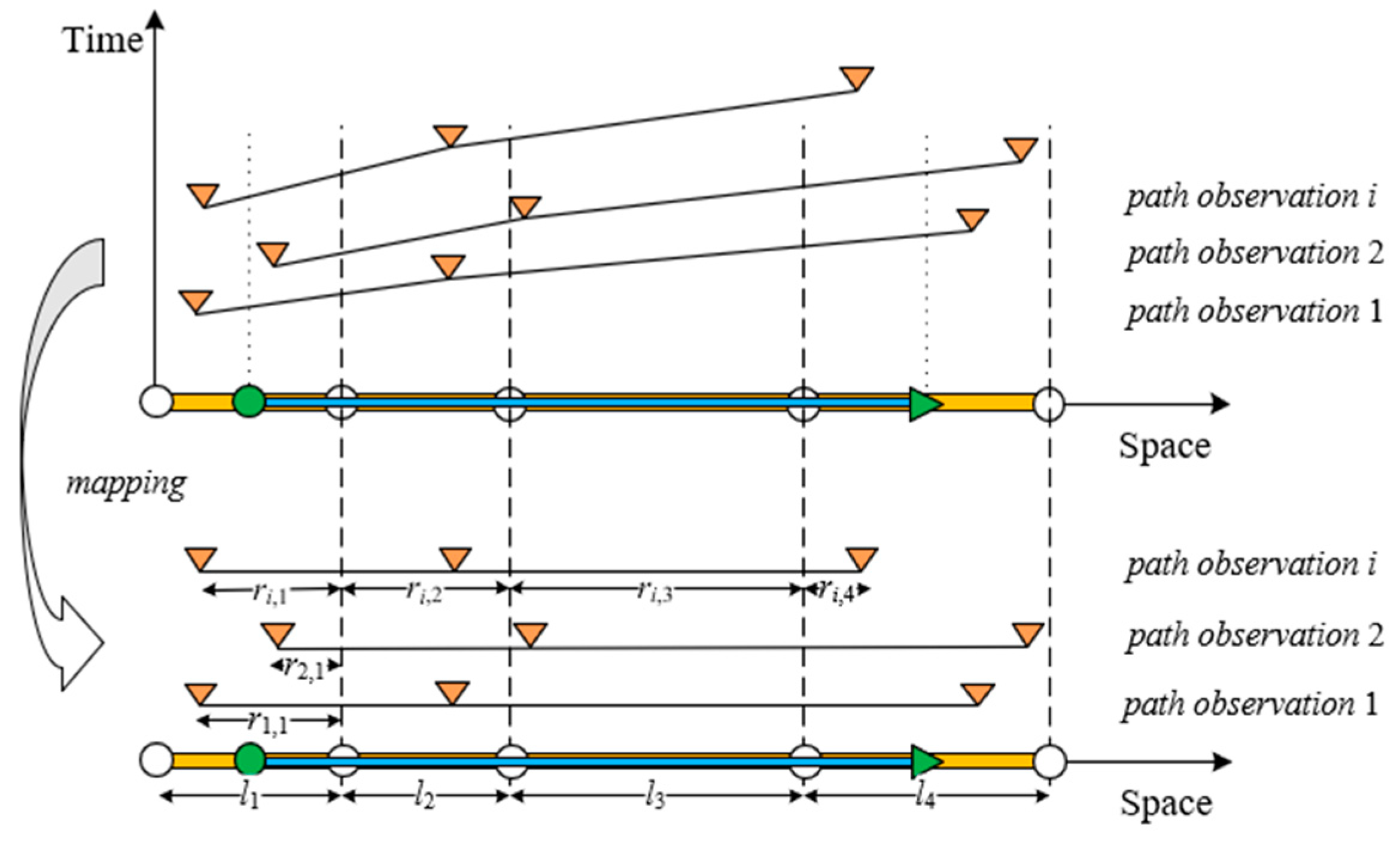
It is assumed that for the road section k where the i-th observation point is located, the length covered by the floating car track is expressed as rik. Then:
According to Formula (2) [29], the coverage degree ρik of the floating car track to the road section k can be expressed as ρik = rik/lk.
(3) The coverage of the floating car track on a single road section to the target path
For the road section k, the coincidence ratio of the trajectory of the floating car and the target path is expressed as βik = min {αk, ρik}.
As can be seen from Figure 2, the object of this study contains three lines: the trajectory of the floating car, the road network path composed of road network nodes and the target path to be calculated. In practice it is almost impossible for these three lines to coincide with each other.
2.3. Information Extraction of Trajectory Data
(1) Track extraction
Step1: cluster tracks with similar trips together to observe the tracks of one group.
Step2: select the track data set covering the target path from the above group, then each track i observation includes a series of interval observations (i1, …, in) composed of GPS data points of floating cars, and the total track length is Li.
(2) The trajectory of the floating car is scaled to the coverage path
Convert the trajectory of the floating car with the covered path as shown in Figure 3, and the conversion factor is ( is the pre-calculated travel time of the road section k).
Map the travel time in the free flow state to the travel time when the floating car passes in equal proportion, including:
where:
τ′i is the travel time of the covered path.
τi is the trajectory travel time of the floating car.
For the i-th observation track:
(3) Zoom the overlay path to the target path
The travel time of the target can be expressed as:
where
ηi is the scaling factor.
ηi is taken as:
(4) Time stamp estimation of access path
Keep the travel time between the first detection point (time stamp si) of the floating car GPS track and the first road network node inside the target path, then:
where:
p′ is the path of the floating car to the first road network node in the target path interval.
The estimated travel time when the starting point of the whole path reaches the first node is:
where:
π′ is the path from the starting point of the path to the first road network node in the target path interval. The path entry timestamp s′i can be estimated as:
3. Estimation and Reliability Calculation of Road Travel Time Distribution after Earthquake
3.1. Road Vulnerability Analysis
Seven factors affecting the seismic performance of roads [30] are: earthquake magnitude, subgrade soil type, site type, foundation failure, subgrade failure, subgrade height difference, and fortification intensity. According to the quantified values of numerous factors affecting road earthquake damage, the curve of road earthquake damage degree after earthquake can be given:
where:
ind is the seismic damage index of a certain test.
θ3 is a normal number, which is the average seismic. is the average earthquake damage index:
where:
Xj is the quantitative value of each influence factor.
In practical application, it is difficult to complete the basic data of the road. Therefore, the damage level of pavement can be judged directly according to the description of quantized value by image recognition technology.
3.2. Impact Factors of Earthquake Damage of Path Travel Time
3.2.1. Evaluation of Road Accessibility after Earthquake
After the earthquake, the accessibility probability Pt of the road is expressed as exponential distribution:
Among them, the value of θ is:
Among them, indk ϵ (0,1] is the seismic damage index of road section k, and is the ideal capacity of road section k under normal conditions, in pcu/h/lane.
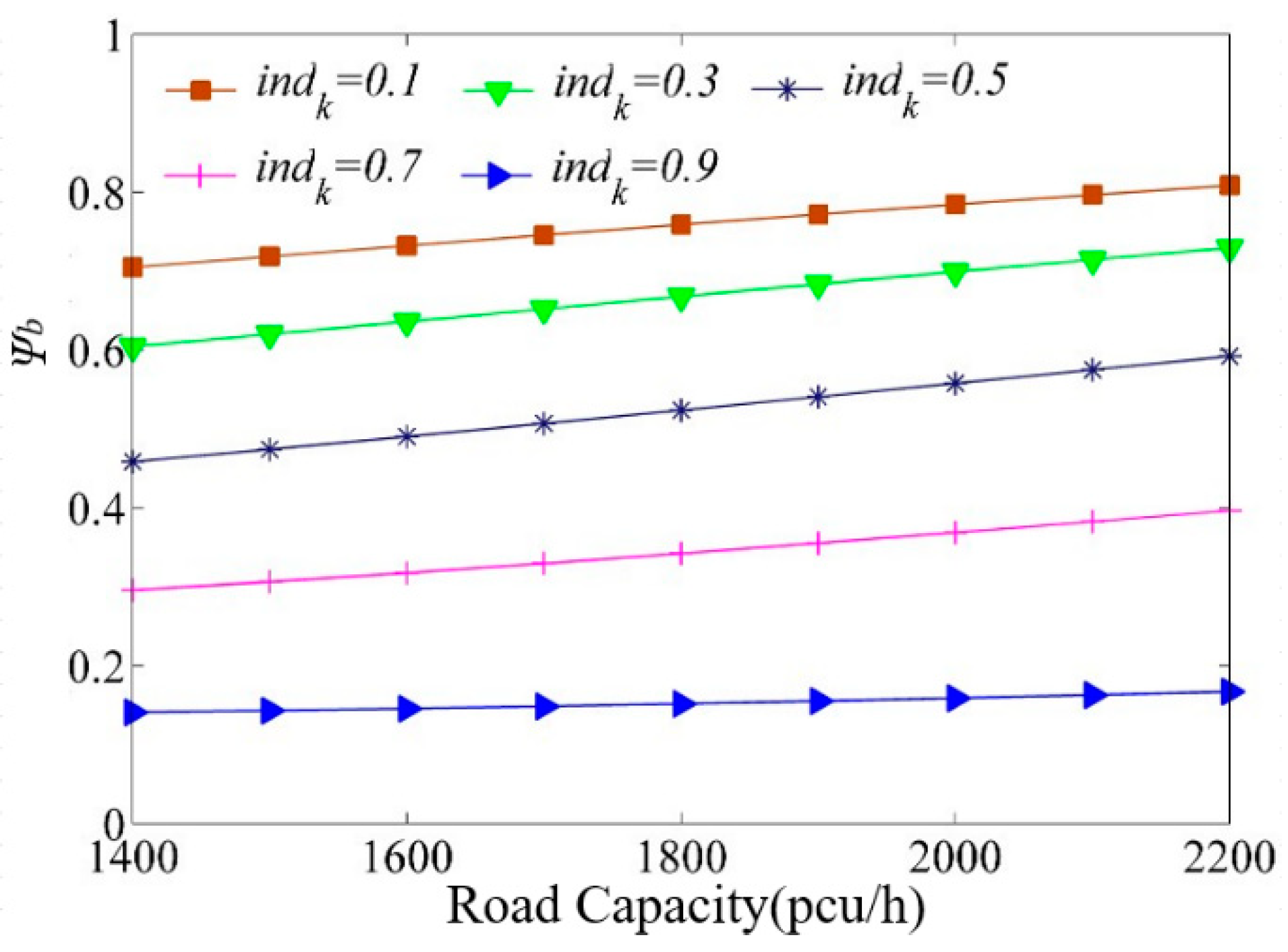
Under the premise of a certain normal traffic capacity, the Q3 values of post-earthquake road sections under different earthquake damage indexes are shown in Figure 3.
Find the 3/4 quantile of post-earthquake capacity C by the distribution function defined by Formula (12):
The traffic Q3 values of sections with different traffic capacity after the earthquake are given in Formula (14). At the same time, the road capacity is analyzed, respectively, from the normal and post-earthquake conditions. The results of the above two examples show that the exponential distribution model is reasonable. According to Figure 3a, when the earthquake damage index increases, the road capacity gradually decreases. According to Figure 3b, under the same earthquake damage index, the greater the basic road capacity of a road, the higher the road capacity is.
3.2.2. Calculation of Earthquake Damage Influencing Factors
The speed V(c) under the ideal capacity of any road is obtained by fitting method. The fitting result is:
Type c is the ideal capacity of the road section (pcu/h/lane).
For a certain road section k, the error between the theoretical travel time after the earthquake and the normal travel time is expressed as:
where:
lk is the length of the road section.
V(·) is the recommended speed value corresponding to the ideal capacity, Q3 is given by Formula (14).
is the road capacity under normal conditions.
Assuming that V() < V(Q3) is constant, after finishing, the Formula (16) is obtained:
Transform Equation (16), and define the seismic impact factor that changes in the interval (0,1) as :
The Formula (18) is substituted into the Formula (17) to obtain:
where:
θ2 is a control parameter greater than zero, θ2 is s/m, and it is obtained by substituting V (·) and Q3 (·).
Figure 4 shows the curves corresponding to different earthquake damage indexes ind under a given θ = 0.3.
3.2.3. Weight of Observation Values
After the ‘Section 2.3 Information extraction from trajectory data’ is completed, the travel time of the path is assigned a weighting coefficient for each observation. This has two advantages: firstly, it can reflect the representability of the observations related to the target path, secondly, it corrects the errors caused by the uneven coverage of the data collected by the floating car.
The Figure 5 and Figure 6 shows the establishment process about the estimation model of traffic travel time by post-earthquake.
After the earthquake, the trajectory of a floating car passing through the target path was obtained (Prb1, Prb2, …, Prb8), the acquired image was recognized, and the earthquake damage influence factors , , …, , the seismic damage influence factor of this trajectory can be obtained.
The weight of observation values is the combination of the influence factor vi of path incomplete coverage, the influence factor λi of road ergodic non-uniformity and the factor of earthquake damage influence, then .
(1) The path incomplete coverage influences factor vi
The influence factor vi of path incomplete coverage is expressed as:
where:
θ1 is a normal number which can influence the degree of change in the incomplete coverage weight of the path.
is distribution factor.
is scaling factor.
(2) Road ergodic non-uniformity factor λi
Assuming that Nk is the observation times for road section k, then:
where [*] is a Gaussian rounding function.
The influence of uneven traversal of the sample road section due to λi can be expressed as:
(3) Earthquake damage influence factor .
The earthquake damage influence factor can be obtained by seismic influence factor in each observation point.
3.2.4. Statistical Eigenvalue Calculation
(1) Central moment calculation
Average value of target travel time:
where:
ωi is the weighted value of travel time of the i-th trajectory observation.
Ti is the travel time observation value converted by the i-th trajectory observation.
The central moment is expressed as:
(2) Percentile calculation
Step1: arranging all observed values Ti from small to large.
Step2: find the [np/100th] number ([*] is the upward rounding operation).
Step3: the [np/100th] number is the p-th quantile.
(3) Estimation of probability density function
In this paper, the latest Bayesian mean adaptive density estimation method (ADEBA) is used [31]. Compared with the previous adaptive probability density estimation method, two parameters ξ and ζ are added, which makes the change in bandwidth H in the kernel density method more consistent with objective laws. Therefore, the travel time probability density function of the target path can be expressed as:
where:
K is the Gaussian kernel function.
In addition, the bandwidth hi is:
where:
ξ and ζ are parameters, which are obtained by grid search.
ωi is the weighted value of travel time of the i-th trajectory observation.
is a prior preliminary estimate of p(x).
3.3. Estimation of Travel Time Distribution after Earthquake
The probability density of the travel time distribution of a path after the earthquake is estimated by the kernel density method. According to Formula (27), the travel time distribution function of the path after the earthquake is:
Calculation of travel time reliability after earthquake.
where:
R is the reliability of travel time.
t is the actual travel time.
t~T, is expected value of Tr and m is the delay time that travelers can endure.
Because of the uncertainty of m, it is taken directly.
where:
Tc is the threshold value, which generally takes the mean value , 1.1 or other fixed value.
4. Analysis of Examples
4.1. Data Acquisition
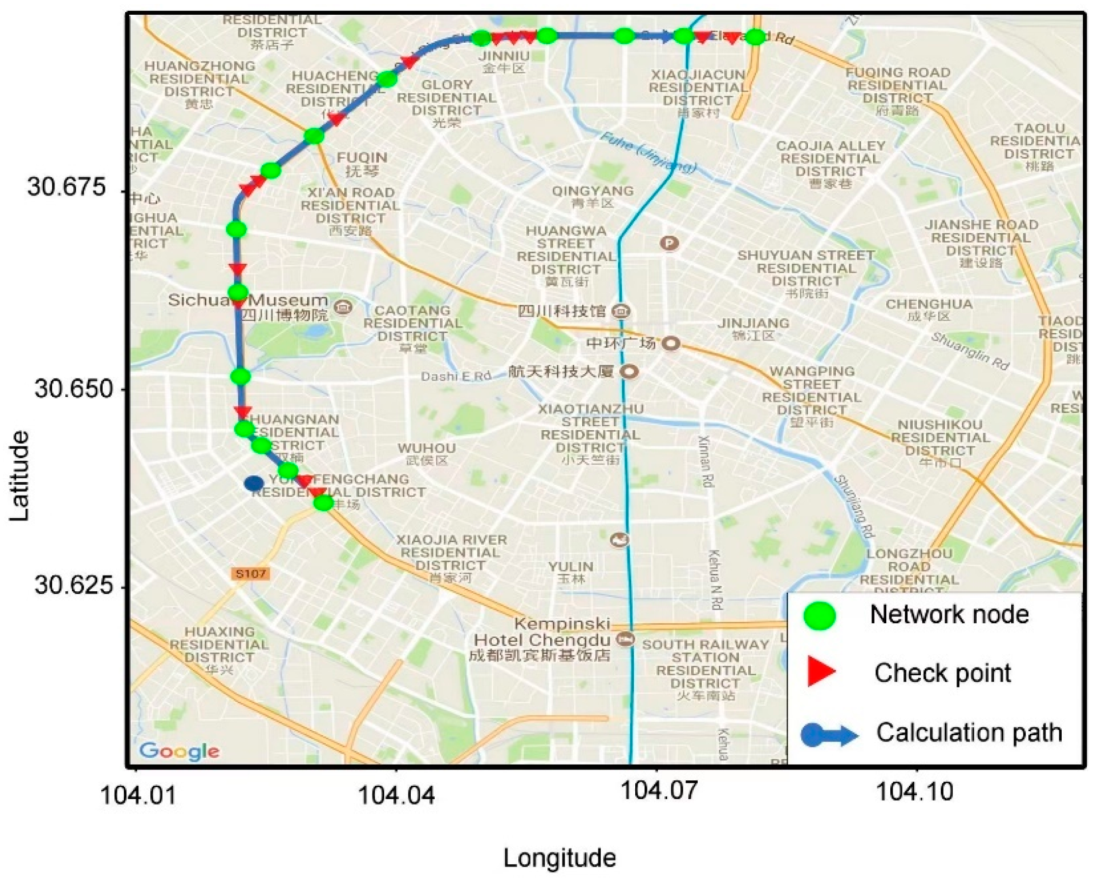
In this paper, a section of the second ring road in Chengdu is selected as the target path. It is 10.5 km long, with a speed limit of 80 km/h and four lanes in both directions, which is one of the main roads in Chengdu. The geographical location of the path is shown in Figure 7.
The authors collected the track records of taxis in Chengdu from 3 August 2014 to 16 August 2014. After data cleaning, abnormal records and duplicate records were removed, and the data during the period from 06:00:00 to 23:59:59 were retained as the floating car data set under normal conditions. VISSIM software was used for simulation to obtain the post-earthquake floating car data set by combining the traffic flow information of this section under normal conditions. Hence, the travel time simulation value of the post-earthquake floating car trajectory was obtained, as shown in Table 2, Table 3 and Table 4. To test the impact of earthquake damage on the reliability of path travel time, this paper assumes that the earthquake damage can be divided into three types: basically intact, medium damage, and destroy, the earthquake damage index is 0.1, 0.5, and 0.9, respectively.
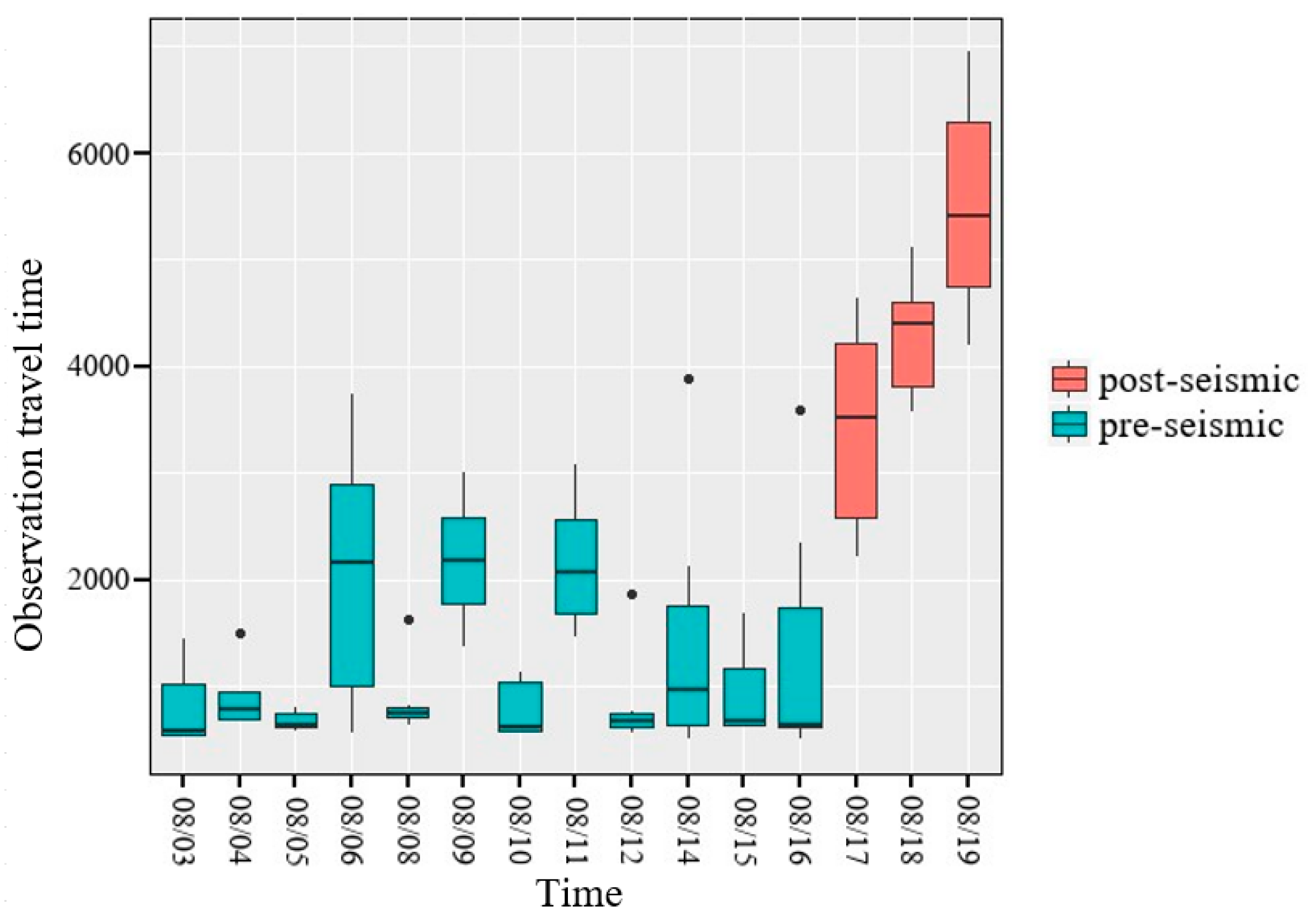
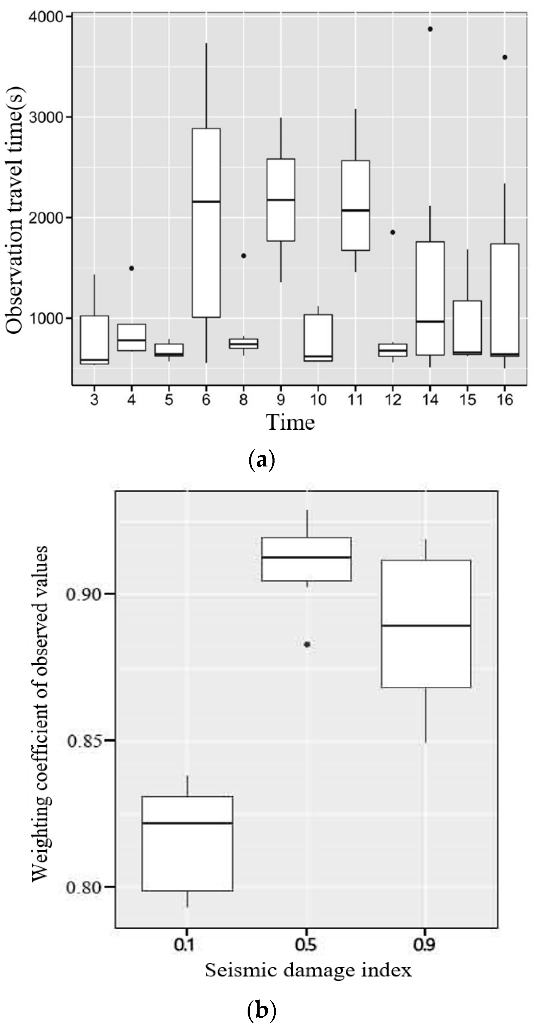
VISSIM software was used to simulate the float track travel time after the earthquake (see Appendix A for float track data set), propose and select the data, obtain float data from 7:00:00 to 9:00:00 and corresponding float track number, and calculate the travel time, as shown in Figure 8.
As can be seen from Figure 8, before the earthquake, the average observed values of floating vehicle track were mostly distributed below 1000 s (approximately equal to 17 min), and 2000 s (approximately equal to 34 min) occurred in some congestion dates. Most of the observed values of the floating vehicle track after the earthquake are distributed in about 4000 s (approximately equal to 67 min), which is basically consistent with that of the actual situation.
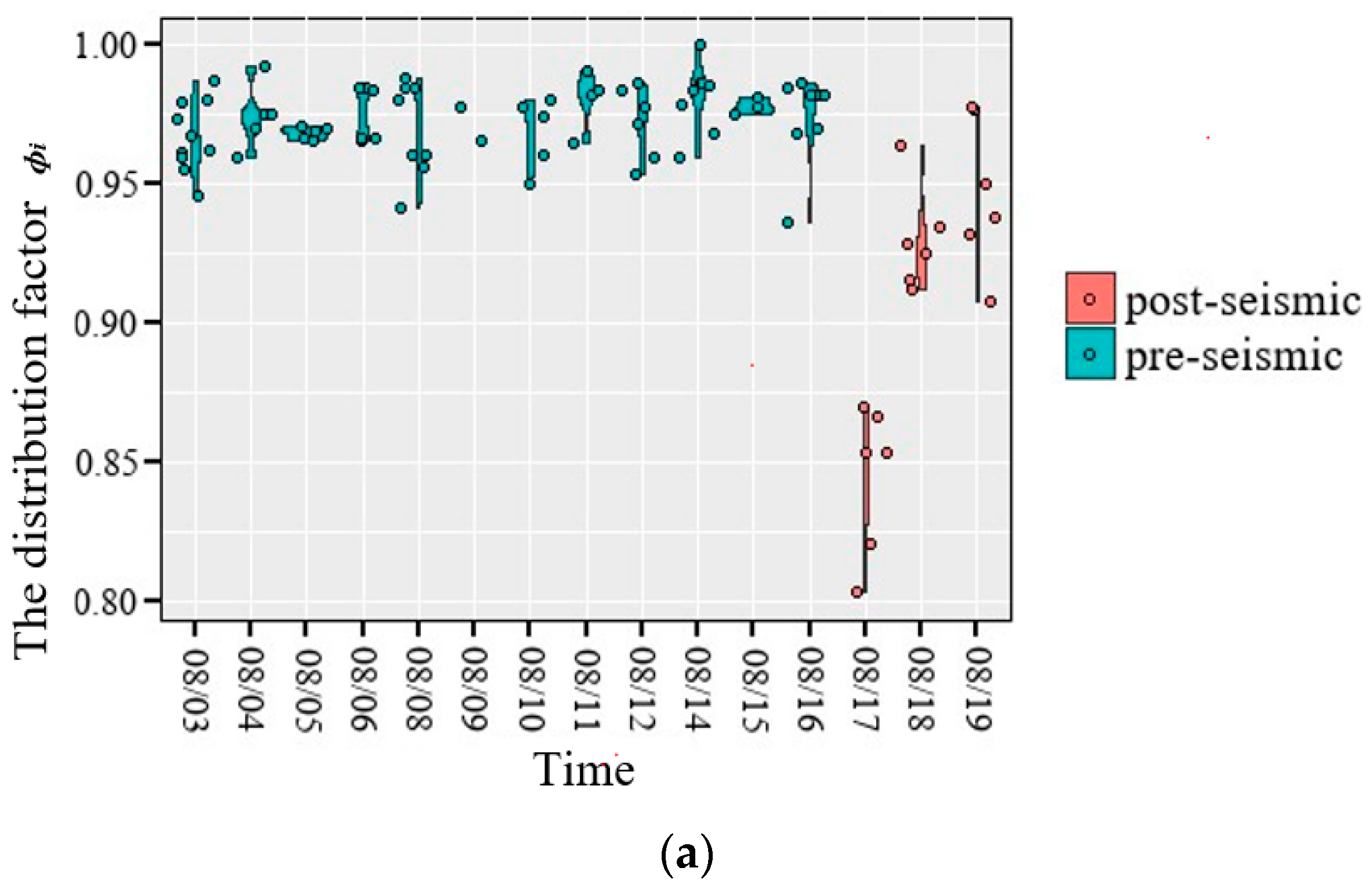
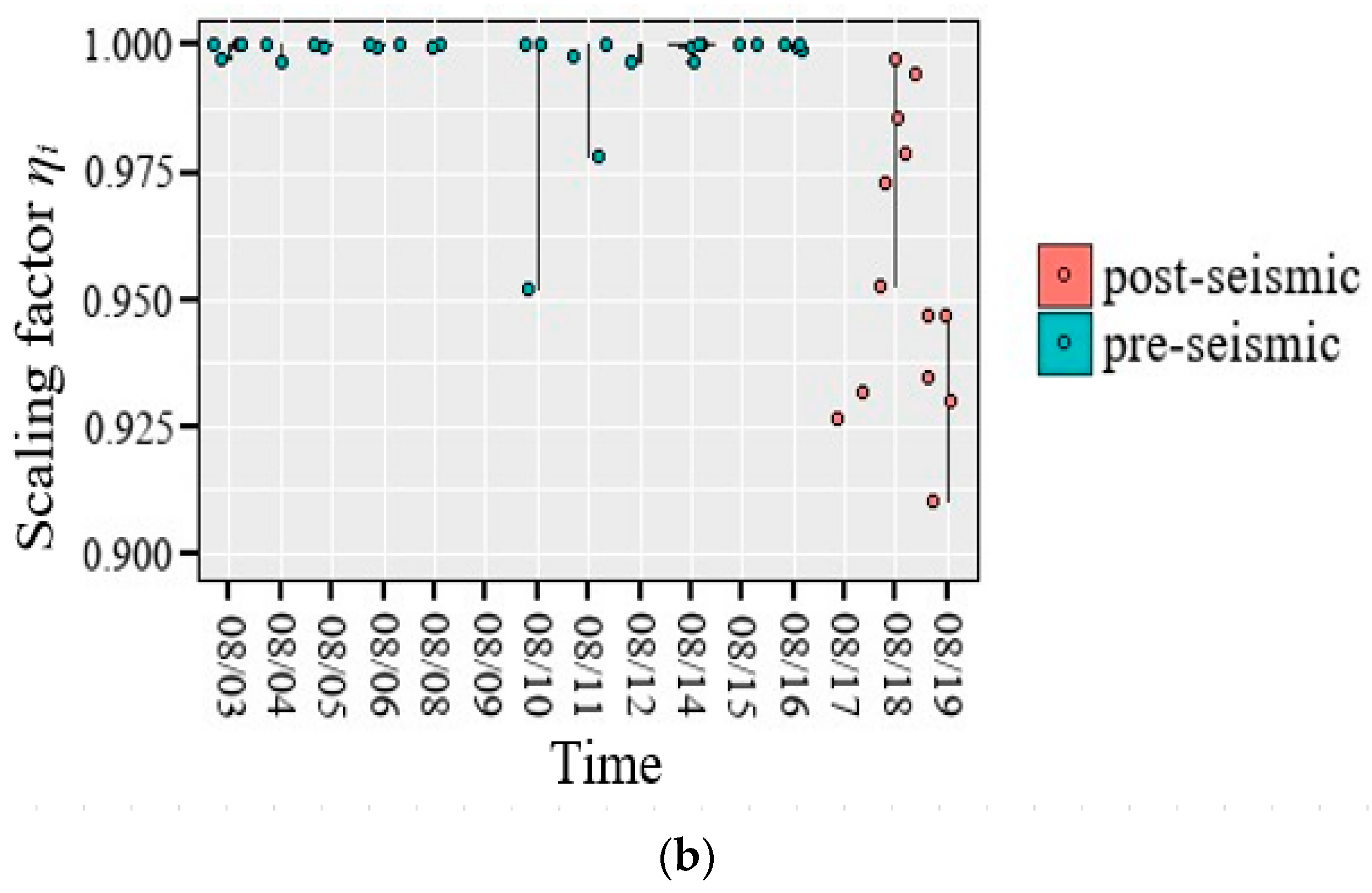
4.2. Calculation of Distribution Factor and Scaling Factor
4.3. Weight Calculation
The function of weights is to describe the influence degree of several factors on the final path travel time distribution, which can reduce the errors caused by incomplete path coverage and uneven path traversal. The results of weighting coefficient ω are shown in Figure 11.
As can be seen from Figure 11a, due to the random distribution of float data overall, the weighting coefficient of float observation value under normal circumstances before the earthquake is evenly distributed, concentrated between 0.190 and 0.1975. It is not difficult to see from Figure 11b that, under the same condition of floating vehicle track, the weight coefficient of the observed value after the earthquake increases significantly compared with that before the earthquake, and different earthquake damage indexes have a great influence on the weight coefficient of the observed value. When the earthquake damage index is 0.1, the weight coefficient of the observed value is distributed between 0.790 and 0.832, and the median is 0.820, showing a left-biased distribution. When the damage index reached 0.9, the weighted coefficient of the observed values ranged from 0.870 to 0.910, with a median of 0.889, showing a right-skewed distribution. When the earthquake damage index was 0.5, the data were more concentrated and distributed between 0.905 and 0.920 with a median of 0.913, presenting a normal distribution. The interquartile interval IQR represents Q3-Q1, and the points in the figure are mild outliers, between Q3+1.5IQR and Q3+3IQR, or between Q1-3IQR and Q1-1.5IQR. In general, the greater the earthquake damage index, the greater the weighted coefficient of observed values.
4.4. Estimation of Probability Density Function
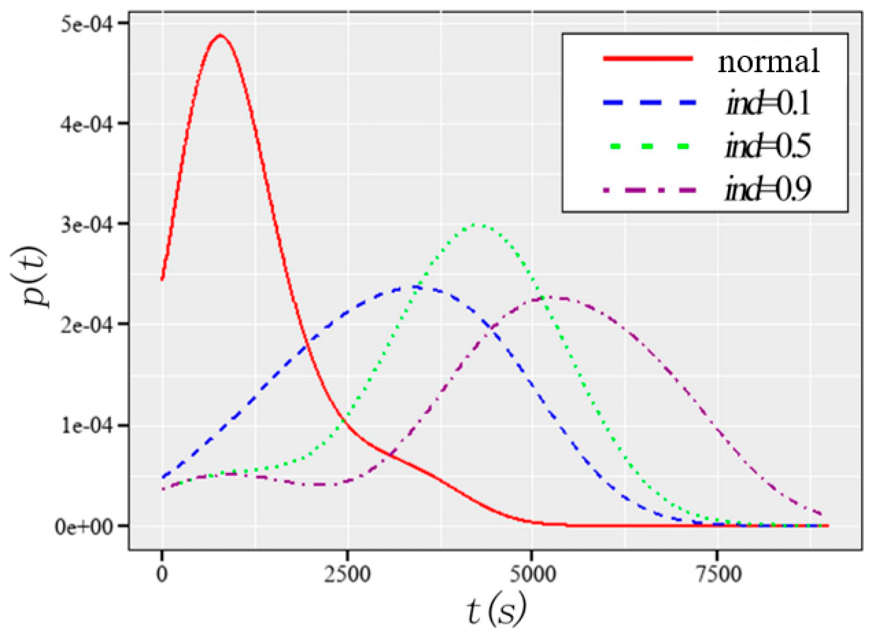
For the estimation of the probability density function of travel time, the results are shown in Figure 12.
From Figure 12, it can be found that the overall probability of wave peak weakening after the earthquake shifts to the direction of long travel time. the pre-earthquake curve reaches its peak at about 1155 s of observation time, namely the probability of 47.6 × 10⁻³, when the earthquake damage index is 0.1, the pre-earthquake curve reaches its peak at about 4652 s of observation time, namely the probability of 44.3 × 10⁻³, the pre-earthquake curve reaches its peak at about 4436 s of observation time. The peak value of the wave is 30.1 × 10⁻³. The peak of the pre-earthquake curve was reached at about 5368 s, and the peak value was 23.2 × 10⁻³ This phenomenon becomes increasingly obvious with the increase in earthquake damage index, which is consistent with the results of qualitative analysis.
4.5. Path Travel Time Reliability Analysis
Table 5 shows the reliability analysis results under different fixed values of path travel time.
It can be seen from the data in Table 5, in the case of a threshold to determine, before the highest path travel time reliability, when the threshold value is 6000, the seismic travel time reliability of road reached 98%, and with the seismic damage index increases, the road travel time is becoming more and more unreliable, when the threshold is 1800, seismic damage index of 0.9, the travel time reliability of this section is only 11%.
5. Conclusions and Discussion
This paper proposes a new method for calculating the travel time reliability after the earthquake based on the analysis and feature processing of the traffic data collected by the floating vehicle. Firstly, this paper defines the relevant intermediate parameters to help convert the travel trajectory of the floating vehicle into the travel time of the target path. Secondly, the impact factors of road earthquake damage are obtained after the image recognition. Besides, Bayesian average adaptive kernel density estimation method are taken many measured trajectories generated by the floating vehicle segments as the data set. Finally, the kernel density estimation method is used to weight the observed values, and the calculation formula of travel time reliability is obtained. Especially, the influence formula of the earthquake on the path travel time distribution is given. The disaster factors which is first applicated in the estimation of the travel time distribution in the research. A complete reliability calculation model of the path travel time after the earthquake is established, which can be used for relevant departments to judge the reliability of road networks and provide effective basis for improving the speed of material transportation and emergency rescue.
(1) According to the track data (time stamp, crossing ratio, coverage area, etc.) of rescue vehicles and the field data analysis, the image recognition technology was used to estimate the earthquake damage condition of the field road, and the calculation formula of the travel time reliability was established based on the estimation of the post-earthquake road travel time distribution. The results show that the Bayesian mean adaptive kernel density estimation method can better estimate the post-earthquake traffic travel time. As for the earthquake damage factor, a new calculation formula is given to judge the influence degree of the earthquake damage factor on the road capacity under different earthquake damage index of 0.9, the travel time reliability of this section is only 11%.
(2) After testing, the authors found that, when the threshold was determined, before the path travel time reliability reached the highest, when the threshold was 6000, the road travel time reliability reached 98%, and with the increase in the earthquake damage index, the road travel time became more and more unreliable. When the threshold was 1800, the earthquake damage.
(3) Earthquake disaster factors are included in the estimation of travel time distribution in this paper, but other factors, such as the improvement of road network traffic conditions brought by road repair and temporary traffic control, also affect the accuracy of the estimation of travel time distribution after earthquake, which need further analysis and research.
(4) The travel time reliability is calculated by using the floating vehicle data and VISSIM simulation data to evaluate the road travel time reliability after the earthquake. However, there is no measured value to compare and explain, to highlight the advantages of this method. Therefore, we will consider the comparison and analysis with other recent methods in the follow-up research to verify the results of the proposed mechanism.
Author Contributions
Data curation, S.W.; Funding acquisition, Y.L.; Investigation, M.L.; Methodology, Y.L. and S.W.; Supervision, M.L.; Validation, X.Z.; Writing—original draft, Y.L.; Writing—review and editing, X.Z. All authors have read and agreed to the published version of the manuscript.
Funding
This research was funded by the National Natural Science Foundation Project of China (Grant No. 51878349).
Institutional Review Board Statement
Not applicable.
Informed Consent Statement
Not applicable.
Data Availability Statement
The data presented in this study are available on request from the corresponding author.
Acknowledgments
The authors are grateful, and thank all those who helped to improve this paper during the research, such as Y.D.’s conceptualization and formal analysis.
Conflicts of Interest
The authors declare no conflict of interest.
Appendix A
Appendix A.1. Main Symbol Table

Table A1.
Main symbol table.
| Symbol | Meaning |
|---|---|
| aik | Coverage length of path section k |
| rik | The length of the floating track to the road section k |
| lk | The length of the road section k |
| αik | Coverage degree of path section k |
| ρik | Coverage degree of floating track on road section k |
| βik | The coverage degree of overlapping path to road section k is the minimum value of αik and ρik. |
| τi | Travel time of the i-th trajectory observation |
| Τ′i | Under the i-th trajectory observation, the calculated travel time of the coincident path |
| Distribution factor under the i-th trajectory observation | |
| ηi | Scaling factor under i-th trajectory observation |
| Ti | Estimated travel time of target path under the i-th trajectory observation |
| t0 ik | Estimated travel time of road section k under the i-th trajectory observation |
| s′i | The estimated time point of the floating car’s entry path under the i-th trajectory observation |
| ωi | Weighting coefficient of observation value under the i-th trajectory observation |
| vi | Influencing factors of incomplete path coverage under the i-th trajectory observation |
| λi | Influencing factors of road ergodic non-uniformity under i-th Trajectory Observation |
| p(t) | Probability density of path travel time distribution in normal state |
| ppost(t) | Probability density of path travel time distribution after earthquake |
Appendix A.2. The Number Code
Box A1. Data screening (R).
#--- First screening 1: through the latitude and longitude range
#y1,y2=[30.643967469460215 30.697711341849764],
#x1.x2=[104.01778221130371,104.07983779907227]
GetFangkuang <- function(allFCDdata_9_10am){
allFCDdata_loglat <- subset(allFCDdata_9_10am, allFCDdata_9_10am$V3>=104.01779& allFCDdata_9_10am$V3<=104.09984&allFCDdata_9_10am$V2>=30.61397& allFCDdata_9_10am$V2<=30.69772,row.names=FALSE)
return(allFCDdata_loglat)
}
#--- Initial screening 2: screening by time interval ---
GetByTimeSection <- function(allFCDdata){
allFCDdata_9_10am <-
subset(allFCDdata,(as.POSIXlt(allFCDdata$V5))$hour>=7&(as.POSIXlt(allFCDdata$V5))$hour<9,row.names=FALSE)⋯⋯# Select the specified data dd, note: the row number is saved after filtering!
return(allFCDdata_9_10am)
}
#--- To determine whether the trajectory passes through the area of the origin and destination (1: passed; 0: Do not pass.) ---
# Input: PointsLonLats---- continuous latitude and longitude points
isQiZhongdian <- function(PointsLonLats){
library(sp)
flag <- 0
isInQidian<- point.in.polygon(PointsLonLats[,1],PointsLonLats[,2],PGON_QIDIAN[,1],PGON_QIDIAN[,2])
isInZhongdian<- point.in.polygon(PointsLonLats[,1],PointsLonLats[,2],PGON_ZHONGDIAN[,1],PGON_ZHONGDIAN[,2])
if(sum(isInQidian)>0 && sum(isInZhongdian)>0){
flag <- 1
}
return(as.logical(flag))
}
#--- Just randomly drop some points from all the trajectories
LinesAfterMonteC <- function(FCDdata){
Ids <- levels(factor(FCDdata$V1))
i_longlineid <- 0
afterlines <- matrix(0, 1, 5)
# Go through each trajectory
for (id in as.numeric(Ids)) {
origin_line <- FCDdata[FCDdata$V1== id,]
if(nrow(origin_line)<4){
next
}
after_line <- aLineAfterMonteC(origin_line)
print(after_line)
afterlines <- rbind(afterlines,as.matrix(after_line))
}
return(afterlines[-1,])# The first row is 0
}
#--------------- Data screening, final judgment -------------
# Input: FCDdata-- floating vehicle trajectory data
# Output: filtered trajectory data
LinesAfterFilter <- function(FCDdata){
library(sp)
Ids <- levels(factor(FCDdata$V1))
i_longlineid <- 0
llineid <- matrix()
# Go through each trajectory
for (id in as.numeric(Ids)) {
tmp_line <- FCDdata[FCDdata$V1== id,]
if(nrow(tmp_line)<3){
next
}
#Assemble LonlatPoints
LonlatPoints<- as.matrix(tmp_line[,3:2])
# Whether through the start and end
isQZ <- isQiZhongdian(LonlatPoints)
# If there is no jump, any distance between two consecutive points less than 2km is true
isApt <- isNoAbrupt(LonlatPoints,1)
# Whether it is long enough, above the threshold is true
isLog<- isLong(LonlatPoints,0)
# Is it from low latitude to high latitude (is the direction, right?)
isDrt <- isDirection(LonlatPoints)
# The above conditions must be met
# Browser[]
if (isLog && isApt && isQZ && isDrt)
{
i_longlineid <- i_longlineid+1
llineid[i_longlineid] <- id
}
}
return(llineid)
References
- Chang, S.E.; Nojima, N. Measuring post-disaster transportation system performance: The 1995 Kobe earthquake in comparative perspective. Transp. Res. Part A Policy Pract. 2001, 35, 475–494. [Google Scholar] [CrossRef]
- El-Anwar, O.; Ye, J.; Orabi, W. Efficient Optimization of Post-Disaster Reconstruction of Transportation Networks. J. Comput. Civ. Eng. 2016, 30, 0887–3801. [Google Scholar] [CrossRef]
- Naranjo, J.E.; Alonso, F.J.; Serradilla, F.; Zato, J.G. Floating Car Data Augmentation Based on Infrastructure Sensors and Neural Networks. IEEE Trans. Intell. Transp. Syst. 2012, 13, 107–114. [Google Scholar] [CrossRef]
- Kong, X.J.; Xia, F.; Ning, Z.; Rahim, A.; Cai, Y.; Gao, Z.; Ma, J. Mobility Dataset Generation for Vehicular Social Networks Based on Floating Car Data. In IEEE Transactions on Vehicular Technology; IEEE: Piscataway, NJ, USA, 2018; Volume 67, pp. 3874–3886. [Google Scholar]
- Shi, Q.; Abdel-Aty, M. Big data applications in real-time traffic operation and safety monitoring and improvement on urban expressways. Transp. Res. Part C Emerg. Technol. 2015, 58, 380–394. [Google Scholar] [CrossRef]
- Ygnace, J.L.; Drane, C. Cellular telecommunication and transportation convergence: A case study of a research conducted in California and in France on cellular positioning techniques and transportation issues. In Proceedings of the 2001 IEEE Intelligent Transportation Systems, Oakland, CA, USA, 25–29 August 2001. [Google Scholar]
- Wang, L.; Wang, C.; Zhang, H.; Fan, Y. Research on Urban Dynamic Traffic Information Collection and Processing Method Based on Floating Car. In Proceedings of the First China Intelligent Transportation Annual Conference, Shanghai, China, June 2005. [Google Scholar]
- Schäfer, R.P.; Thiessenhusen, K.U.; Brockfeld, E.; Wagner, P. A traffic information system by means of real-time floating-car data. In Proceedings of the ITS World Congress. DLR, Chicago, IL, USA, 11–14 October 2002. [Google Scholar]
- Kerner, B.S.; Demir, C.; Herrtwich, R.G.; Klenov, S.L.; Rehborn, H.; Aleksic, M.; Haug, A. Traffic state detection with floating car data in road networks. In Proceedings of the 2005 IEEE Intelligent Transportation Systems, Vienna, Austria, 16 September 2005. [Google Scholar]
- Messelodi, S.; Modena, C.M.; Zanin, M.; De Natale, F.G.; Granelli, F.; Betterle, E.; Guarise, A. Intelligent extended floating car data collection. Expert Syst. Appl. 2009, 36, 4213–4227. [Google Scholar] [CrossRef]
- Jian, S.; Ying, Z.; Chun, Z. OD travel time prediction method based on driver’s route choice preference. J. Traffic Transp. Eng. 2016, 16, 143–149. [Google Scholar]
- Zhang, F.; Zhu, X.; Guo, W.; Hu, T. Sparse Link Travel Time Estimation Using Big Data of Floating Car. Geomat. Inf. Sci. Wuhan Univ. 2017, 42, 56–62. [Google Scholar]
- Zheng, Y.; Zhu, X.; Zhang, F.; Guo, W.; Zhang, D.; Zeng, C. Road Travel Time Estimation Based on Road Network Similarity. Appl. Res. Comput. 2018, 35, 1681–1685. [Google Scholar]
- Wang, Y.; Zheng, Y.; Xue, Y. Travel Time Estimation of a Path using Sparse Trajectories. In Proceedings of the 20th ACM SIGKDD International Conference on Knowledge Discovery and Data Mining (KDD), New York, NY, USA, 24–27 August 2014. [Google Scholar]
- Qiu, J.; Du, L.; Zhang, D.; Su, S.; Tian, Z. Nei-TTE: Intelligent Traffic Time Estimation Based on Fine-Grained Time Derivation of Road Segments for Smart City. In IEEE Transactions on Industrial Informatics; IEEE: Piscataway, NJ, USA, 2020; Volume 16, pp. 2659–2666. [Google Scholar]
- Jenelius, E.; Koutsopoulos, H.N. Travel time estimation for urban road networks using low frequency probe vehicle data. Transp. Res. Part B-Methodol. 2013, 53, 64–81. [Google Scholar] [CrossRef]
- Ma, Z.; Koutsopoulos, H.N.; Ferreira, L.; Mesbah, M. Estimation of trip travel time distribution using a generalized Markov chain approach. Transp. Res. Part C 2017, 71, 1–21. [Google Scholar] [CrossRef]
- Shi, C.; Chen, B.Y.; Li, Q. Estimation of Travel Time Distributions in Urban Road Networks Using Low-Frequency Floating Car Data. ISPRS Int. J. Geo-Inf. 2017, 6, 253. [Google Scholar] [CrossRef]
- Contreras, D.; Blaschke, T.; Kienberger, S.; Zeil, P. Spatial connectivity as a recovery process indicator: The L’Aquila earthquake. Technol. Forecast. Soc. Chang. 2013, 80, 1782–1803. [Google Scholar] [CrossRef]
- Khademi, N.; Balaei, B.; Shahri, M.; Mirzaei, M.; Sarrafi, B.; Zahabiun, M.; Mohaymany, A.S. Transportation network vulnerability analysis for the case of a catastrophic earthquake. Int. J. Disaster Risk Reduct. 2015, 12, 234–254. [Google Scholar] [CrossRef]
- Akbari, V.; Salman, F.S. Multi-vehicle synchronized arc routing problem to restore post-disaster network connectivity. Eur. J. Oper. Res. 2017, 257, 625–640. [Google Scholar] [CrossRef]
- Fang, K.; Fan, J.; Yu, B. A trip-based network travel risk: Definition and prediction. Ann. Oper. Res. 2022. [Google Scholar] [CrossRef]
- Zhang, Z.; Wang, Y.; Chen, P.; He, Z.; Yu, G. Probe data-driven travel time forecasting for urban expressways by matching similar spatiotemporal traffic patterns. Transp. Res. Part C Emerg. Technol. 2017, 85, 476–493. [Google Scholar] [CrossRef]
- Shen, X.; Yang, B. Reliability prediction model of arrival time of road emergency rescue after earthquake. Value Eng. 2016, 35, 184–186. [Google Scholar]
- Hou, B.; Li, X.; Han, Q.; Liu, A.; Lan, R. Connectivity and Travel Time Analysis of Highway Network after Earthquake Based on Monte Carlo Simulation. China J. Highw. Transp. 2017, 30, 287–296. [Google Scholar]
- Fan, J.; Wu, C. New Interpretation and Application of Membership Degree in FCM Algorithm. Acta Electron. Sin. 2004, 350–352. [Google Scholar]
- Xue, X.; Yang, H.; Ren, N. Travel Time Reliability of Regional Road Network under Emergency Conditions. J. Transp. Inf. Saf. 2019, 37, 25–32. [Google Scholar]
- Zhang, Y.; Yin, X.; Mo, Y.; Lin, Y. Research on Survivability of Urban Bus Network Considering Trip Time Reliability. Appl. Res. Comput. 2020, 37, 34–36+40. [Google Scholar]
- Rahmani, M.; Jenelius, E.; Koutsopoulos, H.N. Non-parametric estimation of route travel time distributions from low-frequency floating car data. Transp. Res. Part C Emerg. Technol. 2015, 58, 343–362. [Google Scholar] [CrossRef]
- Li, Y. Model and Method of Earthquake Emergency Decision of Transportation System; Institute of Engineering Mechanics, China Earthquake Administration: Harbin, China, 2014.
- Bäcklin, C.L.; Andersson, C.; Gustafsson, M.G. Self-tuning density estimation based on Bayesian averaging of adaptive kernel density estimations yields state-of-the-art performance. Pattern Recognit. 2018, 78, 133–143. [Google Scholar] [CrossRef]
Figure 1.
FCM clustering results.

Figure 2.
Floating cars trace, network route and target route: (a) Definition of parameters r and a; (b) The relationship among floating vehicle trajectory, road network path, target path and coverage path.
Figure 2.
Floating cars trace, network route and target route: (a) Definition of parameters r and a; (b) The relationship among floating vehicle trajectory, road network path, target path and coverage path.

Figure 3.
Distribution of traffic capacity c after earthquake.

Figure 4.
Calculation of seismic damage influence factor .

Figure 5.
Road network itinerary.

Figure 6.
Mapping process of trace observation.

Figure 7.
Selected route (clockwise direction).

Figure 8.
Travel time obtained from observation data of floating car.

Figure 9.
Distribution factor and scaling factor corresponding to each trajectory observation: (a) Distribution factor; (b) Scaling factor.
Figure 9.
Distribution factor and scaling factor corresponding to each trajectory observation: (a) Distribution factor; (b) Scaling factor.


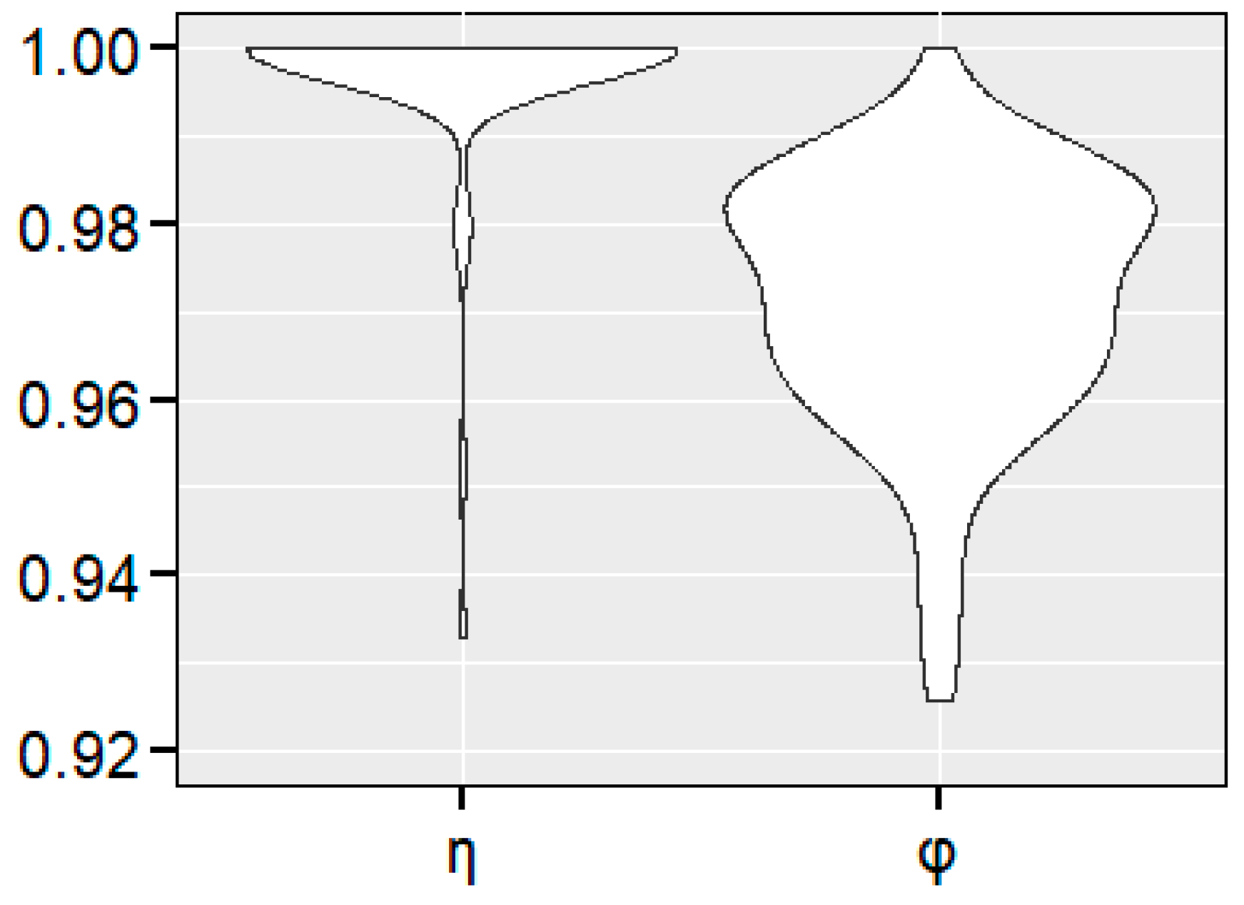
Figure 10.
Distribution factor and scaling factor dispersion of the whole data set.

Figure 11.
Dispersion of weighting coefficients ω: (a) Dispersion of weighting coefficients of normal observation values before earthquakes; (b) Dispersion of weighting coefficients of post-earthquake observation values.
Figure 11.
Dispersion of weighting coefficients ω: (a) Dispersion of weighting coefficients of normal observation values before earthquakes; (b) Dispersion of weighting coefficients of post-earthquake observation values.

Figure 12.
Probability density of path travel time before and after earthquake.

Table 1.
Average velocity value of cluster center.
| Category | Mean Velocity |
|---|---|
| green | 72.556 |
| carmine | 77.182 |
| red | 77.616 |
Table 2.
The simulated FCD set (ind = 0.1).
| Vehicle ID | Start Time of Floating Car Track | End Time of Floating Car Track | The Trajectory Observation Travel Time is Ti/Second | Average Earthquake Damage Index ind |
|---|---|---|---|---|
| 2801 | 17 August 2014 07:41 | 17 August 2014 8:55 | 4429 | 0.1 |
| 2802 | 17 August 2014 08:04 | 17 August 2014 8:41 | 2210 | 0.1 |
| 2803 | 17 August 2014 08:00 | 17 August 2014 9:00 | 3601 | 0.1 |
| 2804 | 17 August 2014 07:43 | 17 August 2014 8:39 | 3412 | 0.1 |
| 2805 | 17 August 2014 08:51 | 17 August 2014 9:29 | 2289 | 0.1 |
| 2806 | 17 August 2014 07:36 | 17 August 2014 8:53 | 4630 | 0.1 |
Table 3.
The simulated FCD set (ind = 0.5).
| Vehicle ID | Start time of Floating Car track | End Time of Floating Car Track | The Trajectory Observation Travel Time is Ti/Second | Average Earthquake Damage Index ind |
|---|---|---|---|---|
| 2807 | 18 August 2014 7:00 | 18 August 2014 8:17 | 4635 | 0.5 |
| 2808 | 18 August 2014 7:05 | 18 August 2014 8:16 | 4268 | 0.5 |
| 2809 | 18 August 2014 7:10 | 18 August 2014 8:25 | 4515 | 0.5 |
| 2810 | 18 August 2014 7:15 | 18 August 2014 8:14 | 3564 | 0.5 |
| 2811 | 18 August 2014 7:20 | 18 August 2014 8:45 | 5113 | 0.5 |
| 2812 | 18 August 2014 7:25 | 18 August 2014 8:26 | 3653 | 0.5 |
Table 4.
The simulated FCD set (ind = 0.9).
| Vehicle ID | Start Time of Floating Car Track | End Time of Floating Car Track | The Trajectory Observation Travel Time is Ti/Second | Average Earthquake Damage Index ind |
|---|---|---|---|---|
| 2813 | 19 August 2014 7:00 | 19 August 2014 8:55 | 6943 | 0.9 |
| 2814 | 19 August 2014 7:05 | 19 August 2014 8:14 | 4198 | 0.9 |
| 2815 | 19 August 2014 7:10 | 19 August 2014 8:58 | 6520 | 0.9 |
| 2816 | 19 August 2014 7:15 | 19 August 2014 8:31 | 4592 | 0.9 |
| 2817 | 19 August 2014 7:20 | 19 August 2014 8:47 | 5222 | 0.9 |
| 2818 | 19 August 2014 7:25 | 19 August 2014 8:58 | 5606 | 0.9 |
Table 5.
Path Travel Time Reliability under Different Threshold.
| Tc (s) | Before the Earthquake (%) | Ind = 0.1 (%) | ind = 0.5 (%) | ind = 0.9 (%) |
|---|---|---|---|---|
| 1800 | 44 | 25 | 16 | 11 |
| 3000 | 92 | 63 | 51 | 47 |
| 6000 | 98 | 97 | 82 | 58 |
Publisher’s Note: MDPI stays neutral with regard to jurisdictional claims in published maps and institutional affiliations. |
© 2022 by the authors. Licensee MDPI, Basel, Switzerland. This article is an open access article distributed under the terms and conditions of the Creative Commons Attribution (CC BY) license (https://creativecommons.org/licenses/by/4.0/).
Share and Cite
MDPI and ACS Style
Li, Y.; Wang, S.; Zhang, X.; Lv, M. Estimation and Reliability Research of Post-Earthquake Traffic Travel Time Distribution Based on Floating Car Data. Appl. Sci. 2022, 12, 9129. https://doi.org/10.3390/app12189129
AMA Style
Li Y, Wang S, Zhang X, Lv M. Estimation and Reliability Research of Post-Earthquake Traffic Travel Time Distribution Based on Floating Car Data. Applied Sciences. 2022; 12(18):9129. https://doi.org/10.3390/app12189129
Chicago/Turabian StyleLi, Yongyi, Shiqi Wang, Xiaorui Zhang, and Mengxing Lv. 2022. "Estimation and Reliability Research of Post-Earthquake Traffic Travel Time Distribution Based on Floating Car Data" Applied Sciences 12, no. 18: 9129. https://doi.org/10.3390/app12189129
Note that from the first issue of 2016, this journal uses article numbers instead of page numbers. See further details here.