
Deep Transfer Learning-Based Fault Diagnosis Using Wavelet Transform for Limited Data


1
Defense & Safety ICT Research Department, Electronics and Telecommunications Research Institute, Daejeon 34129, Korea
2
Department of Information Engineering, Computer Science and Mathematics, University of L’Aquila, 67100 L’Aquila, Italy
3
Dental Clinic Center, Kyungpook National University, Daegu 41940, Korea
4
Department of Radio and Information Communications Engineering, Chungnam National University, Daejeon 34134, Korea
*
Author to whom correspondence should be addressed.
Appl. Sci. 2022, 12(15), 7450; https://doi.org/10.3390/app12157450
Submission received: 5 July 2022
/
Revised: 21 July 2022
/
Accepted: 22 July 2022
/
Published: 25 July 2022
Abstract
:Although various deep learning techniques have been proposed to diagnose industrial faults, it is still challenging to obtain sufficient training samples to build the fault diagnosis model in practice. This paper presents a framework that combines wavelet transformation and transfer learning (TL) for fault diagnosis with limited target samples. The wavelet transform converts a time-series sample to a time-frequency representative image based on the extracted hidden time and frequency features of various faults. On the other hand, the TL technique leverages the existing neural networks, called GoogLeNet, which were trained using a sufficient source data set for different target tasks. Since the data distributions between the source and the target domains are considerably different in industrial practice, we partially retrain the pre-trained model of the source domain using intermediate samples that are conceptually related to the target domain. We use a reciprocating pump model to generate various combinations of faults with different severity levels and evaluate the effectiveness of the proposed method. The results show that the proposed method provides higher diagnostic accuracy than the support vector machine and the convolutional neural network under wide variations in the training data size and the fault severity. In particular, we show that the severity level of the fault condition heavily affects the diagnostic performance.
1. Introduction
Fault diagnosis is a crucial component of modern industrial systems since early and accurate fault diagnosis not only ensures operational reliability and safety but also reduces maintenance costs [1,2,3]. Recently, the research on data-driven fault diagnostics has grown and developed considerably, thanks to the vast amount of data obtained from the Industrial Internet of Things [4,5]. In particular, the deep learning-based diagnosis technique is one of the most promising and powerful tools for detecting and diagnosing various industrial faults since it automatically learns the hidden features from historical data [4,6].
However, training a deep learning-based fault diagnosis model from scratch is computationally expensive and requires substantial amounts of training data to have a sufficient generalization capacity [7,8,9]. In most practical industrial scenarios, the training data are strictly limited, and the generation of realistic training samples is not always feasible, since some critical components of the machines are not allowed to operate even with minor faults. Furthermore, collecting large labeled data is a time-consuming and labor-intensive procedure [10].
On the other hand, transfer learning (TL) is a fundamental deep learning technique that allows reuse of the trained model, learned from the source domain, with different target domains [7]. Specfically, TL can provide a good performance by overcoming the limited training data of the fault diagnosis [11]. However, leveraging the existing model, trained on large source data to the target domain, is still challenging since the source and target domains are conceptually different tasks in most industrial scenarios. The data distribution of the industrial target domain can be significantly different from one of the well-known existing image classifications of the source domain, such as ImageNet.
This paper combines wavelet transform and TL to diagnose the industrial faults using limited target samples. The main contributions of the paper are as follows:
- We adopt a pre-trained model, GoogLeNet, to classify industrial faults where the wavelet transformation converts one-dimensional time-series data into two-dimensional images of the time and frequency domains as the input. To deal with the constraints of the limited target samples, we first partially retrain the pre-trained model using the intermediate data that are conceptually related to the target domain, but less expensive, to collect the samples. We then retrain this relatively small portion of the pre-trained intermediate model using the target data.
- We extensively evaluate the effectiveness of the proposed method and compare it with the state of the art. We use a Simulink model of a triplex reciprocating pump with different fault combinations and severity levels. The proposed method improves the generalization capability to classify the fault types while reducing the dependency on the training data of the source domain. In particular, we show the critical impact of the severity level on the fault classification accuracy.
The remainder of the paper is organized as follows. Section 2 discusses the related works. Section 3 details the proposed method combining wavelet transform and TL. Section 4 presents the experimental data set and the state-of-the-art methods for a comparative analysis. Section 5 evaluates the performance of the proposed method through an extensive set of experiments. Finally, Section 6 summarizes the overall contributions and discusses the future direction of the research.
2. Related Works
Due to the significant advantage of automatic feature extraction, various deep learning models, such as auto-encoder [10], the Recurrent Neural Network (RNN) [12], and the Convolutional Neural Network (CNN) [13,14], have been investigated for fault detection and diagnosis problems. Janssens et al. [13] adopted a CNN model to automatically extract features and enable classification of the bearing fault. However, various operating conditions of industrial environments seriously degrade the effectiveness of the deep learning-based fault detection and diagnosis method [1,3]. Zhang et al. [14] integrated a CNN model with training interference and varying kernel dropout using the raw time-series signal as the input. The data augmentation further improves the classification accuracy of the extended CNN model under various operating conditions. Azamfar et al. [15] developed a two-dimensional CNN model, which uses the frequency spectrum obtained from multiple sensors as the input for the bearing fault diagnosis.
Most deep learning models need a large amount of training data in order to train [7,8]. However, faulty industrial data are costly to collect because crucial components or equipment in manufacturing systems are not permitted to operate in faulty states. Further, the distribution of sensor measurements, even for the same equipment, varies depending on the operating conditions. Moreover, conventional augmentation methods make generating realistic training samples difficult due to the complex non-linear operations of industrial machines [16].
As one of the most promising techniques, TL leverages the rich capability of the source domain to facilitate the industrial target model using the fine-tuning or adaptation for the fault detection and diagnosis problem [17]. Xie et al. [9] proposed a fusion method for bearing fault classification without having a strong knowledge of feature engineering or the large training samples of deep learning models. The XGBoost classifier is trained with two types of features, namely, predetermined empirical features and adaptive features provided by LiftingNet. LiftingNet adaptively extracts the hidden features for the target task that depend on noise and working conditions. To enhance the sparsity and the adaptive feature’s learning of limited data, Li et al. [10] adopted the parameter TF to construct their model of the multiple stacked non-negativity constraint sparse autoencoders for the rolling bearing fault diagnosis. Zhang et al. [18] developed a few-shot learning method in which the pre-trained Siamese neural network is extended with wide first-layer kernels to conduct the rolling bearing fault diagnosis. Sauf et al. [19] proposed a sparse autoencoder-based fault diagnosis method in which the particle swarm optimization method provides the optimal hyperparameters of the architecture. Kurtogram images are used to train the proposed model to implement fault diagnosis.
However, the TL model may only provide a low prediction accuracy of the target domain due to the significant domain discrepancy between the source and target domains in practical fault diagnosis scenarios. In our work, we introduce the intermediate domain, which is conceptually similar to the target domain, to partially retrain the pre-trained network model. Moreover, the wavelet transform provides the frequency spectrum characteristics of the time-varying measurements. Further, we extensively evaluate the effectiveness of the proposed method using various fault combinations and severity levels of the complex reciprocating pump model, while most existing studies use relatively simple bearing faults.
3. Wavelet-Based Deep Transfer Learning
This section presents the framework based on the wavelet transform and the TL model.
3.1. Overall Framework
This section proposes a wavelet-based deep TL method to address the fault diagnosis problem using limited target samples. Figure 1 presents the proposed framework consisting of the pre-trained GoogLeNet, which uses the source data, and the partial retraining of the same pre-trained model, which uses the intermediate data and the target data. The continuous wavelet transform (CWT) constructs the time and frequency characteristics of the time-series signal and generates the image of the intermediate and target data.
The major components of the proposed framework are as follows:
- Pre-trained model: We use the GoogLeNet trained on the ImageNet data set to classify 1000 categories of the typical images [20]. GoogLeNet is a 22-layer CNN, a variant of the inception network developed at Google for image classification and object detection.
- Training on the intermediate domain: The CWT converts the time-series signals of the intermediate domain to the wavelet images capturing the time and frequency characteristics. The intermediate network has nearly the same architecture as the pre-trained model of the source domain. Some subsequent parameters of the network are updated using the intermediate samples, while we reduce the amount of learning parameters to avoid overfitting by fixing most of the parameters of the preceding layers. Once the network is trained, it is used as the general fault diagnosis model to input the wavelet images.
- Training on the target domain: Similarly, CWT converts the time-series signals of the target domain to the wavelet images in terms of the time and frequency domains. The limited wavelet images of the target domain are passed to the intermediate network to fine-tune a few subsequent layers of the network for the fault diagnosis of the target domain.
- Fault diagnosis stage: The target network is eventually utilized to classify various fault types based on the extracted feature information of the wavelet images.
3.2. Wavelet Transformation
Various faults deteriorate the power spectrum characteristic of the signal in the temporal period rather than the stationary behavior [21]. Thus, it is necessary to jointly investigate the signal characteristics of the time and frequency domains.
The CWT separates the signal into several frequency components, and each component is then evaluated by the appropriate scale [22,23]. It efficiently analyzes the abrupt transient behavior of industrial signals with rapidly changing frequencies over the slowly varying behavior [24]. Similar to the Fourier transform, the CWT essentially measures the similarity between a signal and a basis function called a wavelet, [23]. By integrating the scaling parameter a and the translating parameter b, a continuous wavelet function is obtained
The CWT is basically defined as the inner product between the signal and the wavelet function , namely,
where is the complex conjugate of , and is the inner product [23]. Each coefficient is multiplied by the correctly scaled and shifted wavelet to produce the constituent wavelets of the signal.
By varying the values of the scales a and the positions b, we obtain the CWT coefficients as a function of two variables from the time-series signals with a size of , as shown in Figure 1. The abrupt transitions are separable from smoother signal features since these result in large absolute values of the wavelet coefficients.
Finding the optimal size of the image depends upon the capacity of the original signal and the computational complexity. While the computational complexity is generally proportional to N, decreasing the value of N incurs a significant loss of the features. In this paper, we set and scale it to as the input image for the pre-trained GoogLeNet [20].
3.3. Deep Transfer Learning
In Figure 1, TL is used to classify the wavelet image obtained by CWT for which only limited target samples are available for the fault diagnosis. We denote the large-scale labeled fault data of the source domain as in which and are the source sample within a specific feature space and the corresponding label of the label space , respectively. On the other hand, the target domain contains a small, labeled sample set in which and are the target sample and the corresponding label, respectively. For instance, we consider the ImageNet data as the source domain and the wavelet images of the faulty data as the target domain.
Due to the domain discrepancy, the probability distribution of the source domain and that of the target domain are considerably different, . Since the number of target data is strictly limited, it does not capture the essential features of various fault types. Moreover, the label spaces of the machine health conditions are considerably different from the general image detection and recognition of the source domain. Thus, the source network model requires sophisticated tuning procedures to apply to the target domain.
On the other hand, some data sets, such as bearing faults, are publicly available even though they may not be directly related to the target domain [25]. Moreover, we could simulate various fault scenarios of industrial machines to collect the measurements [1]. We define this data, relevant to the target domain, as the intermediate domain. We denote the intermediate data as where and are the intermediate sample and the corresponding label, respectively. Considering the domain discrepancy, the probability distribution of the intermediate domain is assumed to be closer to that of the target distribution than that of the source distribution , where M denotes the similarity between probability distributions, such as the Bhattacharyya distance [26]. The number of the intermediate data is assumed to be greater than that of the target data, .
In Figure 1, the pre-trained GoogLeNet is partially retrained using the new set of wavelet images of the intermediate domain to obtain the intermediate network model. The earlier layers extract the common features of images, such as blobs, edges, and colors, while the later layers concentrate on more explicit features to classify data sets. Thus, the parameters of the few later layers of the network are only updated using the intermediate samples as the training data set. Moreover, we set the learning rates of several initial layers of the pre-trained network model to zero. By doing this, the learning speed improves, since the gradients of the fixed layers do not need to be computed. In GoogLeNet in Figure 2, we freeze the first 14 layers, including the inception (4c), while we retrain the rest of the layers from the inception (4d) module. To prevent overfitting, we add the dropout layer after the last average pooling layer of the network. The dropout layer randomly assigns the input component to zero with a certain probability. The last fully connected layer is customized to the intermediate domain.
The network parameters of the intermediate model are then transferred to the target domain. The wavelet images of the target domain are used to train the network layers. We use almost the same architecture as that of the intermediate network, except for the last classification layer and the number of fixed layers. The number of filters of the last fully connected layer equals the size of the classes of the target domain. Furthermore, fixing earlier layers prevents overfitting due to the strictly limited target samples. Thus, we increase the number of fixed layers to the first 17 layers, including the inception (4e) module. In the training process, we set the size of the batch sample to 1280 and the number of epochs to 3000. We use the Adam optimizer [27], the first-order gradient-based optimization algorithm of the stochastic objective functions, based on adaptive estimates of the lower-order moments, with a learning rate of . The model training and testing are performed on the computer with the Intel Xeon Platinum 8270 processor and the Nvidia RTX A6000 GPU.
4. Evaluation Setup
This section details the experimental data sets and the state-of-the-art methods of fault diagnosis for the comparative analysis.
4.1. Fault Data
We consider the sufficient samples of the bearing fault data as the intermediate domain, and the limited samples of the pump model are used as the target domain. We use the triplex reciprocating pump model of the Simulink since it allows us to run different fault combinations and severity levels with detailed working conditions [28]. We refer to the detailed description of the bearing fault data of the intermediate domain in [25].
This section describes the experimental data generated using the reciprocating pump model to evaluate the effectiveness and feasibility of the proposed method under limited target data [28]. The triplex reciprocating pump consists of the pump housing, crank, and plungers. The pump model is configured to generate three common types of faults, namely, cylinder leaks, blocked inlet, and increased bearing friction. Thus, the number of possible fault types is eight, including one healthy state without any faults, three of a single fault, three combinations of two faults, and one with three simultaneous faults. Table 1 describes the details of these eight classes, labeled as of the target domain used in this study. Due to the noise of the model, we obtain different simulation outputs even with the same fault parameters. Each sample of the pump model comprises 1201 output flow data values at the sampling rate of 1000 Hz.
We consider different severity ranges of cylinder leaks , blocked inlet , and bearing friction based on the specifications of the pump model. Each range of the fault types is divided into nine severity levels. We set as the healthy state . We obtain 400 samples for the given fault type and the severity level. Thus, the total number of samples per fault types is equal to where 9 corresponds to the number of severity levels of each fault type. We also generate the equal number of samples as the healthy state .
The data sets are split into the ratio of as training, validation, and testing sets. We randomly shuffle and select the samples of each class to build each data set. We vary the ratio of the training data set in order to evaluate the impact of the size of the training data.
4.2. Comparison
As a comparison with the TL-based fault diagnosis method, we apply two common classification models, SVM and CNN, for our fault diagnosis problems. We refer to our approach as CNN–TL to distinguish the CNN model trained from scratch.
- SVM: A machine learning technique known as SVM relies on the structural risk minimization problem [29]. It can perform well in a high-dimensional non-linear problem with limited samples. Various signal processing techniques for the time and frequency domains are adopted to manually extract the features of the signals. We use various statistical metrics of the time domain analysis, including mean, standard deviation, root mean square, kurtosis, maximum-to-minimum difference, and signal median absolute deviation. Furthermore, the spectral analysis extracts useful features for predicting faults, such as bearings, gears, and engines [21]. We consider the cumulative powers in the low-frequency range of 10–20 , mid-frequency range of 40–60 , and high-frequency range above 100 , as well as the frequency of the peak magnitude and spectral kurtosis peak. Note that spectrum condition indicators of various frequency ranges are based on the expected harmonics due to the specifications of the triplex reciprocating pump model, as we will discuss in Section 5.
- CNN: Figure 3 depicts the structure and the configuration of the CNN, consisting of 18 layers. The hidden layer mainly consists of the convolutional layer, the batch normalization layer, the activation layer, the sub-sampling layer, and the dropout layer. We adopt the rectified linear units (ReLUs) as an activation function to improve the training time. The output of the convolutional layer is fed to the max pooling of the sub-sampling layer. The softmax function is applied to the output of the last fully connected layer and returns the distribution of eight class labels corresponding to the fault types. The classification accuracy of the CNN considerably depends on the configuration parameters, including input image size, activation function, filter size, sampling method, and iteration number. The network parameter optimization method is adopted to optimize the configuration parameters for the classification accuracy [30].
5. Performance Evaluation
In this section, we first analyze the characteristics of the signals of the triplex reciprocating pump model in the time and frequency domains. We then evaluate the fault diagnosis performance of our proposed method.
5.1. Fault Data Analysis
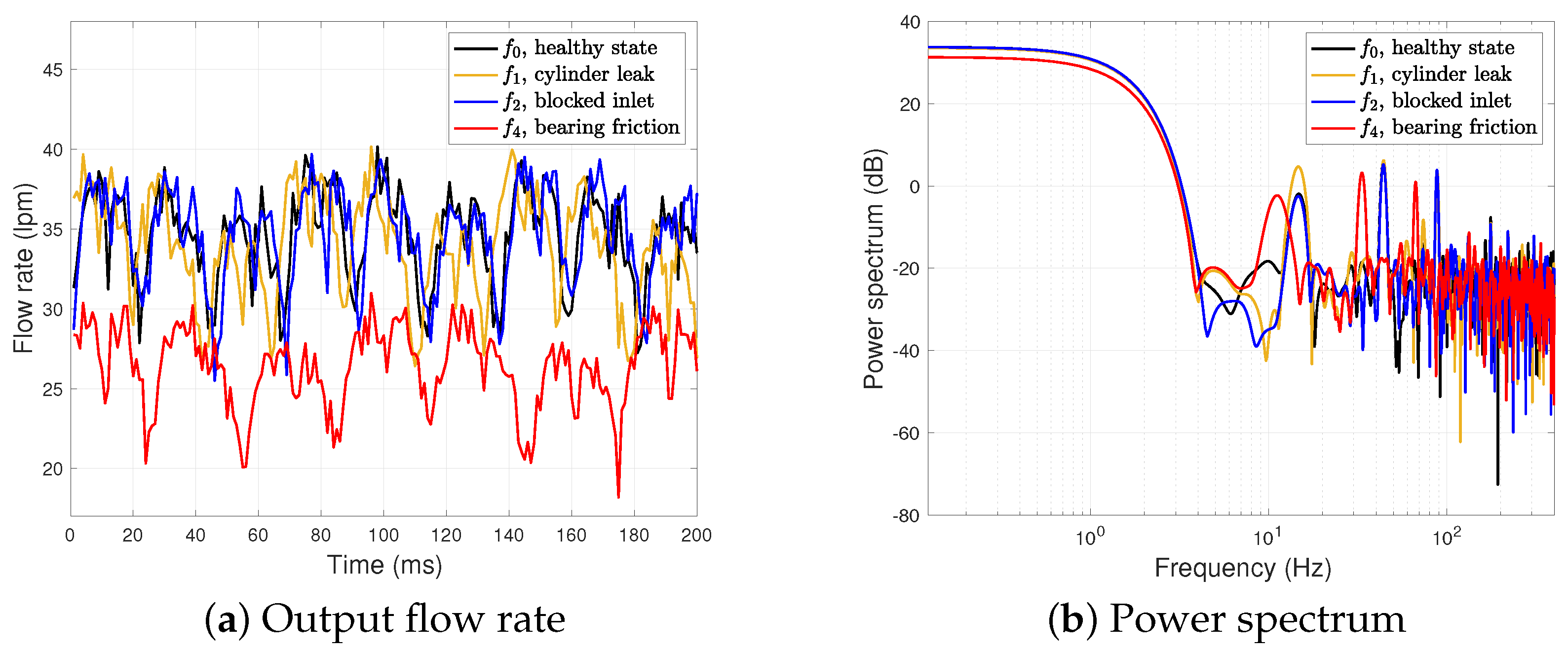
Figure 4 depicts the output flow rate and the power spectrum of the healthy state and three different types of a single fault, and , as shown in Table 1. The faults and correspond to the single fault type due to cylinder leak, blocked inlet, and increased bearing friction, respectively. Note that the unit of the volumetric flow rate is the liters per minute (lpm). We set the severity level for all faults.
In Figure 4a, the overall shapes of the output flow rates are similar between and , while the bearing friction fault heavily decreases the output flow rate. Thus, the time domain analysis of the industrial signals is not enough to characterize each fault type.
Some of the effects of different fault types are more noticeable in the spectrum analysis of the frequency domain, as shown in Figure 4b. The power spectrum includes several resonant peaks. In particular, since the triplex pump model has three cylinders, it inherently has peaks at , or , as well as harmonics at multiples of where corresponds to the inverse of the pump motor speed, . The faults of and have three peaks at and while has three slightly shifted peaks. The power spectrum value of at is higher than those of and . Thus, it shows that the characteristics of both time and frequency domains are critical for classifying the fault types. However, it is still not trivial to distinguish and even in the power spectrum.
Next, we analyze how the severity level of the fault condition affects the signal in both the time and frequency domains. Figure 5 presents the output flow rate and the power spectrum of the healthy state and the blocked inlet fault with different severity levels . We also report two output flow rates of the healthy state due to different noise realizations.
In Figure 5a, two outputs of and three outputs of with different severity levels are very similar in the time domain. On the other hand, Figure 5b shows that the high severity level affects the characteristics of the power spectrum. The blocked inlet fault with the severe condition results in several peaks at a high frequency of greater than . Furthermore, it also increases the power by around . However, the minor fault conditions with still have a power spectrum similar to that of the healthy state , making the fault diagnosis difficult. Note that the simulation parameter related to the blocked inlet with is , closer to the threshold of the healthy state, which is . Thus, we observe that the severity level could affect the fault classification performance even with the same fault type.
To further illustrate the time and frequency characteristics of different faults, we show the wavelet images of various fault types with a fixed severity level of in Figure 6. Remember that the CWT technique converts the time-series signals into time-frequency images. We note that the wavelet of the same fault type could be different due to the different realization of the noise.
Three horizontal narrow stripes of and correspond to three peaks of the power spectrum around 15.8 , 47.4 , and 2 × 47.4 , which are comparable to Figure 4. We also observe that the lower stripe of around is relatively stronger than those of and . Moreover, two horizontal stripes of are slightly lower than those of and , which are consistent with Figure 4. Thus, the wavelet efficiently captures the characteristics of both the time and frequency domains.
Let us consider the wavelet images of and where these faults are related to the bearing friction fault , as described in Table 1. The combined fault between the blocked inlet and bearing friction, , is hard to differentiate from the single bearing friction fault due to its minor effect on the blocked inlet. However, the cylinder leak heavily affects the overall wavelet images of and . Thus, the effect of the fault combination is not always obvious due to complex interactions between the different faults.
5.2. Diagnosis Performance Analysis
Figure 7 shows the confusion matrices of three classification models, namely, SVM, the CNN, and CNN–TL with . It summarizes the fault diagnosis results of each fault type, including the healthy state and faulty states . We set the severity level as the fault condition of each fault type. The longitudinal and transverse axes present the true and predicted labels, respectively. The diagonal entries indicate the number of correctly predicted fault types, while the off-diagonal entries are the number of incorrectly predicted fault types. A normalized row value (resp. normalized column value) shows the percentages of correctly and incorrectly classified observations for each true class (resp. each predicted label). Overall, the classification accuracy of the CNN–TL is , which is higher than and of SVM and the CNN, respectively.
One interesting observation is that the confusion matrix has the form of the tridiagonal matrix, and the off-diagonal entries are not fully spread. It means most classification errors tend to be more pairwise than independent random errors. Let us first consider the healthy state and the blocked inlet fault . In the confusion matrix, some faults between and using SVM are incorrectly classified, while the corresponding errors are very low for the CNN and CNN–TL. In Figure 4, we have shown that the healthy state and the blocked inlet fault have similar characteristics in both the time and frequency domains. However, both the CNN and CNN–TL models efficiently handle the classification between and .
Now, we consider the pair of for which most errors of both and are isolated from other fault types. SVM erroneously classifies the cylinder leak fault to the combined cylinder leak and blocked inlet fault when the effect of the blocked inlet is not severe. We also observe similar classification errors of to for the SVM model. Remember that we observe similar wavelet images between and in terms of the positions and the number of horizontal stripes in Figure 6. Both the CNN and CNN–TL reduce the classification errors of to , while the CNN model still has the low classification accuracy of due to the large number of classification errors of , similar to that of SVM. Thus, the classification errors are asymmetric even in the same pair of for the CNN and CNN–TL.
One of the major classification errors is related to the bearing friction fault , namely, and . These pairwise errors are separated from since the corresponding part of the confusion matrix has the form of a block matrix. The two dominant pairs of classification errors are and . The cylinder leak fault makes a noticeable difference between these two pairs, as shown in Figure 6. The classification errors in each pair of and considerably depend on the severity level of the blocked inlet. The CNN–TL still performs better than other models for these pairs. The average accuracy related to of SVM, the CNN, and CNN–TL are and , respectively.
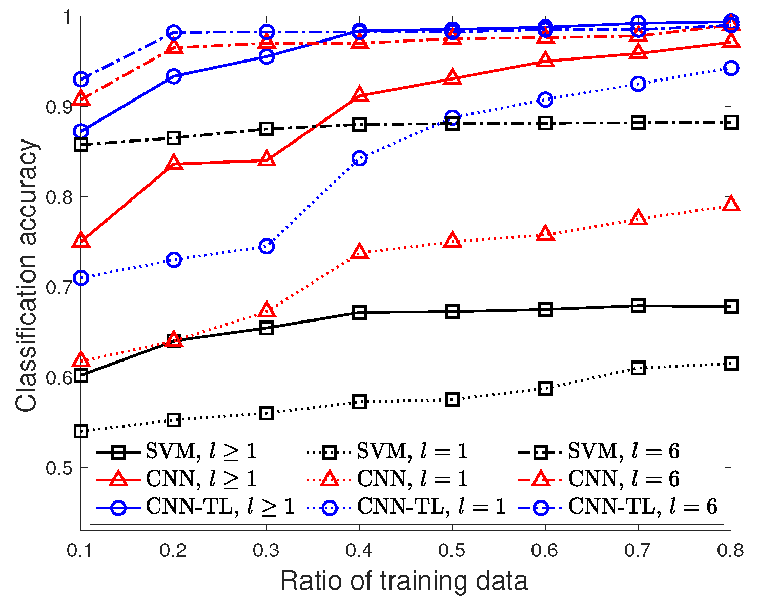
Next, we investigate the performances of the three classification models when limited samples with different severity levels are adopted to train the network. Thus, the ratio of training target samples varies from to . Note that we fix the ratio of the validation and testing data set as . Figure 8 shows the classification accuracy of SVM, the CNN, and CNN–TL with different severity levels as a function of various ratios of training data. The fault condition of is the general scenario in which each fault type contains various samples with different severity levels, while shows how the different severity levels affect the overall classification accuracy.
Let us first consider the general fault condition of with the mixed severity levels in each fault type. Overall, the classification accuracy of all models improves as the number of training samples increases. While both the CNN and CNN–TL improve the classification accuracy by adding more training data, the classification accuracy of SVM is low, around , even with the large training data. SVM’s performance is fundamentally limited due to the manual feature extraction.
Both the CNN and CNN–TL have a good classification accuracy of greater than when they have sufficient training samples: and , respectively. However, under the strictly limited training samples of , the corresponding classification accuracy of the CNN is significantly degraded to , while that of the CNN–TL is still around . The gap between the CNN and CNN–TL increases as the number of training data decreases. The classification accuracy of CNN–TL gradually tends to increase with the addition of more training data, while that of the CNN certainly improves for . When the training sample is insufficient to train the CNN model, it leads to poor performance due to overfitting. The classification accuracy of the CNN–TL is at , which is close to that of the one using the maximum training data . We note that the average training time of CNN–TL (resp. CNN) increases from to (resp. from to ) with the addition of more training data .
Different severity levels, , significantly affect the classification accuracy. For the severe fault condition of , the classification accuracy of the three classification models is greater than , even with the small training samples . However, when the fault becomes minor, , the performances of the different models varies considerably depending on the training data. CNN–TL still provides a classification accuracy of , while the CNN has a low accuracy of for the small training samples . The fault diagnosis with a low severity level is crucial to achieving early fault detection since the impact of the fault is naturally worse due to the fault’s propagation over time. This shows the effectiveness of CNN–TL when the training data of the CNN is not enough to learn the hidden features of the minor fault condition.
To investigate the impact of the severity level, Figure 9 presents the classification accuracy of the three classification models with different ratios of the training data as a function of the various severity levels . Generally, the classification accuracy of the three classification models improves as the fault condition becomes severe due to its significant impacts on the time and frequency domains.
The three classification models perform well for the severe fault condition , while the accuracy trends are considerably different as the fault condition becomes minor. CNN–TL provides better classification accuracy than the other two models for all of the considered ranges of severity levels. Specifically, the worst fifth percentiles of the classification accuracy of SVM, the CNN, and CNN–TL with (resp. ) are , and (rep. ), respectively. Thus, CNN–TL shows a significant benefit when predicting the fault type, even if the fault condition is minor.
Another interesting observation is that adding more training samples does not considerably improve the classification accuracy of SVM, while it still improves the performance of the CNN. The classification accuracy of the CNN is closer to that of SVM for when the training data is small . On the other hand, CNN–TL achieves a high accuracy of greater than for , even with the strictly limited samples .
One of the fundamental issues of the deep learning-based fault diagnosis is the heavy demand of the training data to meet certain classification accuracy, since the amount of training data substantially impact the classification performance. Figure 10 presents the required number of training data with the different accuracy demands of the three classification models as a function of various severity levels . Given the severity level, we compute the required number of training data based on all of the considered ratios of the training data. We set low accuracy demands for SVM since the high classification accuracy is not achievable even with sufficient training data.
Overall, the required training samples decrease as the fault condition becomes severe for the three classification models. As a key insight, the proposed CNN–TL requires fewer training samples, and therefore less training time, to meet a certain accuracy demand compared to other models. In particular, the required number of training samples of the CNN is considerably large as the accuracy demand becomes more strict. CNN–TL requires numerous training samples for the minor fault condition , while the CNN does not even meet the accuracy demands of , even when using all available training samples . SVM fails to meet the demands of for . CNN–TL provides early fault detection at the cost of more training data. However, the number of training samples is still less than that of the CNN model.
6. Conclusions
This paper combines the wavelet transform and TL to diagnose industrial faults using limited target samples. The wavelet transform converts a one-dimensional time-series sample into a two-dimensional time-frequency image by extracting the hidden time and frequency domain characteristics of various faults as the input data to enhance the feature learning ability. To deal with limited target samples and the domain discrepancy between the source and target domains, we adopt the TL framework where we partially retrain the pre-trained model of the source domain using the intermediate samples that are conceptually similar to the target domain but less expensive to collect. We use a Simulink model of a triplex reciprocating pump with various fault combinations and severity levels to evaluate the performance of the proposed method. The proposed fault diagnosis method precisely classifies different single fault types and achieves the highest classification accuracy among SVM and the CNN. In particular, the classification accuracy improves as the fault condition becomes severe due to its significant impacts on the time and frequency domains. On the other hand, the results show that the combined faults are challenging to detect due to the complex interactions between the different faults and severity levels. Furthermore, the required number of training samples required to meet the accuracy demands of the proposed CNN–TL is lower than those required for SVM and the CNN.
We plan to develop the optimization technique to decide the retraining portion of the TL model based on the similarity between the intermediate and target domains and the number of available intermediate samples to improve the classification accuracy and computational efficiency.
Author Contributions
Conceptualization, J.B. and P.P.; Formal analysis, P.P.; Investigation, H.S. and P.P.; Methodology, J.B. and P.D.M.; Software, P.P.; Validation, P.D.M.; Writing—original draft, P.P.; Writing—review & editing, J.B., P.D.M. and H.S. All authors have read and agreed to the published version of the manuscript.
Funding
This work was supported by the research fund of Chungnam National University.
Institutional Review Board Statement
Not applicable.
Informed Consent Statement
Not applicable.
Data Availability Statement
Not applicable.
Conflicts of Interest
The authors declare no conflict of interest.
References
- Rai, A.; Kim, J.M. A novel health indicator based on information theory features for assessing rotating machinery performance degradation. IEEE Trans. Instrum. Meas. 2020, 69, 6982–6994. [Google Scholar] [CrossRef]
- Chen, J.; Li, Z.; Pan, J.; Chen, G.; Zi, Y.; Yuan, J.; Chen, B.; He, Z. Wavelet transform based on inner product in fault diagnosis of rotating machinery: A review. Mech. Syst. Signal Process. 2016, 70–71, 1–35. [Google Scholar] [CrossRef]
- Cerrada, M.; Snchez, R.V.; Li, C.; Pacheco, F.; Cabrera, D.; Valente de Oliveira, J.; Vsquez, R.E. A review on data-driven fault severity assessment in rolling bearings. Mech. Syst. Signal Process. 2018, 99, 169–196. [Google Scholar] [CrossRef]
- Khan, S.; Yairi, T. A review on the application of deep learning in system health management. Mech. Syst. Signal Process. 2018, 107, 241–265. [Google Scholar] [CrossRef]
- Park, P.; Ergen, S.C.; Fischione, C.; Lu, C.; Johansson, K.H. Wireless network design for control systems: A survey. IEEE Commun. Surv. Tutor. 2018, 20, 978–1013. [Google Scholar] [CrossRef]
- Liu, R.; Yang, B.; Zio, E.; Chen, X. Artificial intelligence for fault diagnosis of rotating machinery: A review. Mech. Syst. Signal Process. 2018, 108, 33–47. [Google Scholar] [CrossRef]
- Liu, J.; Ren, Y. A general transfer framework based on industrial process fault diagnosis under small samples. IEEE Trans. Ind. Inform. 2021, 17, 6073–6083. [Google Scholar] [CrossRef]
- Zhang, T.; Chen, J.; Xie, J.; Pan, T. SASLN: Signals augmented self-taught learning networks for mechanical fault diagnosis under small sample condition. IEEE Trans. Instrum. Meas. 2021, 70, 1–11. [Google Scholar] [CrossRef]
- Xie, J.; Li, Z.; Zhou, Z.; Liu, S. A novel bearing fault classification method based on XGBoost: The fusion of deep learning-based features and empirical features. IEEE Trans. Instrum. Meas. 2021, 70, 1–9. [Google Scholar] [CrossRef]
- Li, X.; Jiang, H.; Zhao, K.; Wang, R. A deep transfer nonnegativity-constraint sparse autoencoder for rolling bearing fault diagnosis with few labeled data. IEEE Access 2019, 7, 91216–91224. [Google Scholar] [CrossRef]
- Cao, P.; Zhang, S.; Tang, J. Preprocessing-free gear fault diagnosis using small datasets with deep convolutional neural network-based transfer learning. IEEE Access 2018, 6, 26241–26253. [Google Scholar] [CrossRef]
- An, Z.; Li, S.; Wang, J.; Jiang, X. A novel bearing intelligent fault diagnosis framework under time-varying working conditions using recurrent neural network. ISA Trans. 2020, 100, 155170. [Google Scholar] [CrossRef]
- Janssens, O.; Slavkovikj, V.; Vervisch, B.; Stockman, K.; Loccufier, M.; Verstockt, S.; Van de Walle, R.; Van Hoecke, S. Convolutional neural network based fault detection for rotating machinery. J. Sound Vib. 2016, 377, 331–345. [Google Scholar] [CrossRef]
- Zhang, W.; Li, C.; Peng, G.; Chen, Y.; Zhang, Z. A deep convolutional neural network with new training methods for bearing fault diagnosis under noisy environment and different working load. Mech. Syst. Signal Process. 2018, 100, 439–453. [Google Scholar] [CrossRef]
- Azamfar, M.; Singh, J.; Bravo-Imaz, I.; Lee, J. Multisensor data fusion for gearbox fault diagnosis using 2-d convolutional neural network and motor current signature analysis. Mech. Syst. Signal Process. 2020, 144, 106861. [Google Scholar] [CrossRef]
- Lv, H.; Chen, J.; Zhang, T.; Hou, R.; Pan, T.; Zhou, Z. SDA: Regularization with cut-flip and mix-normal for machinery fault diagnosis under small dataset. ISA Trans. 2021, 111, 337–349. [Google Scholar] [CrossRef]
- Yosinski, J.; Clune, J.; Bengio, Y.; Lipson, H. How transferable are features in deep neural networks? In Proceedings of the International Conference on Neural Information Processing Systems, Montreal, BC, Canada, 8–13 December 2014; pp. 3320–3328. [Google Scholar]
- Zhang, A.; Li, S.; Cui, Y.; Yang, W.; Dong, R.; Hu, J. Limited data rolling bearing fault diagnosis with few-shot learning. IEEE Access 2019, 7, 110895–110904. [Google Scholar] [CrossRef]
- Saufi, S.R.; Ahmad, Z.A.B.; Leong, M.S.; Lim, M.H. Gearbox fault diagnosis using a deep learning model with limited data sample. IEEE Trans. Ind. Inform. 2020, 16, 6263–6271. [Google Scholar] [CrossRef]
- Szegedy, C.; Liu, W.; Jia, Y.; Sermanet, P.; Reed, S.; Anguelov, D.; Erhan, D.; Vanhoucke, V.; Rabinovich, A. Going deeper with convolutions. In Proceedings of the IEEE Conference on Computer Vision and Pattern Recognition, Boston, MA, USA, 7–12 June 2015; pp. 1–9. [Google Scholar]
- Park, P.; Marco, P.D.; Shin, H.; Bang, J. Fault Detection and Diagnosis Using Combined Autoencoder and Long Short-Term Memory Network. Sensors 2019, 19, 4612. [Google Scholar] [CrossRef] [Green Version]
- Abdelgayed, T.S.; Morsi, W.G.; Sidhu, T.S. A new approach for fault classification in microgrids using optimal wavelet functions matching pursuit. IEEE Trans. Smart Grid. 2018, 9, 4838–4846. [Google Scholar] [CrossRef]
- Tran, M.Q.; Liu, M.K.; Tran, Q.V.; Nguyen, T.K. Effective fault diagnosis based on wavelet and convolutional attention neural network for induction motors. IEEE Trans. Instrum. Meas. 2022, 71, 1–13. [Google Scholar] [CrossRef]
- Abdeljaber, O.; Avci, O.; Kiranyaz, M.S.; Boashash, B.; Sodano, H.; Inman, D.J. 1-d CNNs for structural damage detection: Verification on a structural health monitoring benchmark data. Neurocomputing 2018, 275, 1308–1317. [Google Scholar] [CrossRef]
- Bechhoefer, E. Rolling Element Bearing Fault Diagnosis Data. Mathworks Inc., 2018. Available online: https://github.com/mathworks/RollingElementBearingFaultDiagnosis-Data (accessed on 21 July 2022).
- Zhou, S.; Chellappa, R. From sample similarity to ensemble similarity: Probabilistic distance measures in reproducing kernel hilbert space. IEEE Trans. Pattern Anal. Mach. Intell. 2006, 28, 917–929. [Google Scholar] [CrossRef]
- Kingma, P.; Ba, J. Adam: A Method for Stochastic Optimization. In Proceedings of the International Conference on Learning Representations, San Diego, CA, USA, 7–9 May 2015; pp. 1–6. [Google Scholar]
- Miller, S. Triplex Pump with Faults. Mathworks Inc., 2020. Available online: https://github.com/mathworks/Simscape-Triplex-Pump (accessed on 21 July 2022).
- Wang, S.S.; Chern, A.; Tsao, Y.; Hung, J.W.; Lu, X.; Lai, Y.H.; Su, B. Wavelet speech enhancement based on nonnegative matrix factorization. IEEE Signal Process. Lett. 2016, 23, 1101–1105. [Google Scholar] [CrossRef] [Green Version]
- Snoek, J.; Larochelle, H.; Adams, R.P. Practical Bayesian Optimization of Machine Learning Algorithms. In Proceedings of the International Conference on Neural Information Processing Systems, Lake Tahoe, NV, USA, 3–8 December 2012; pp. 2951–2959. [Google Scholar]
Figure 1.
Proposed framework of fault diagnosis using limited target samples.

Figure 2.
GoogLeNet architecture. Conv and FC denote the convolutional layer and the fully-connected layer while MaxPool and AveragePool are the max pooling layer and average pooling layer, respectively; means the filter size of the convolutional layer or the pooling size of the pooling layer, respectively. We add the dropout layer after the last average pooling layer.

Figure 3.
Designed CNN architecture trained from scratch: means c filters with the size of .

Figure 4.
Output flow rate and power spectrum of .

Figure 5.
Output flow rate and power spectrum of and with different severity levels, .

Figure 6.
Wavelet images of different fault types, .

Figure 7.
Confusion matrix of SVM (a), the CNN (b), and CNN–TL with various fault types, (c).

Figure 8.
Classification accuracy of SVM, the CNN, and CNN–TL with different ratios of the training data, .
Figure 8.
Classification accuracy of SVM, the CNN, and CNN–TL with different ratios of the training data, .

Figure 9.
Classification accuracy of SVM, the CNN, and CNN–TL with different severity labels, .

Figure 10.
Required number of training samples of SVM, the CNN, and CNN–TL with different severity labels, .
Figure 10.
Required number of training samples of SVM, the CNN, and CNN–TL with different severity labels, .


Table 1.
Description of 8 different classes of the triplex reciprocating pump model.
| Label | Classes | Number of Samples | Number of Samples |
|---|---|---|---|
| per Severity Level | |||
| healthy state | 3600 | − | |
| cylinder leak | 3600 | 400 | |
| blocked inlet | 3600 | 400 | |
| cylinder leak and blocked inlet | 3600 | 400 | |
| bearing friction | 3600 | 400 | |
| cylinder leak and bearing friction | 3600 | 400 | |
| blocked inlet and bearing friction | 3600 | 400 | |
| cylinder leak and blocked inlet and bearing friction | 3600 | 400 |
Publisher’s Note: MDPI stays neutral with regard to jurisdictional claims in published maps and institutional affiliations. |
© 2022 by the authors. Licensee MDPI, Basel, Switzerland. This article is an open access article distributed under the terms and conditions of the Creative Commons Attribution (CC BY) license (https://creativecommons.org/licenses/by/4.0/).
Share and Cite
MDPI and ACS Style
Bang, J.; Di Marco, P.; Shin, H.; Park, P. Deep Transfer Learning-Based Fault Diagnosis Using Wavelet Transform for Limited Data. Appl. Sci. 2022, 12, 7450. https://doi.org/10.3390/app12157450
AMA Style
Bang J, Di Marco P, Shin H, Park P. Deep Transfer Learning-Based Fault Diagnosis Using Wavelet Transform for Limited Data. Applied Sciences. 2022; 12(15):7450. https://doi.org/10.3390/app12157450
Chicago/Turabian StyleBang, Junseong, Piergiuseppe Di Marco, Hyejeon Shin, and Pangun Park. 2022. "Deep Transfer Learning-Based Fault Diagnosis Using Wavelet Transform for Limited Data" Applied Sciences 12, no. 15: 7450. https://doi.org/10.3390/app12157450
Note that from the first issue of 2016, this journal uses article numbers instead of page numbers. See further details here.