
Two-Layer Matrix Factorization and Multi-Layer Perceptron for Online Service Recommendation


1
School of Computer Science and Engineering, Ningbo University of Technology, Ningbo 315211, China
2
College of Computer Science, Nanjing University of Posts and Telecommunications, Nanjing 210046, China
3
Southwest Institute of Electronic Technology, Chengdu 610036, China
4
College of Computer Science, Tsinghua University, Beijing 100084, China
5
School of Computing and Information Technology, University of Wollongong, Wollongong, NSW 2522, Australia
*
Author to whom correspondence should be addressed.
Appl. Sci. 2022, 12(15), 7369; https://doi.org/10.3390/app12157369
Submission received: 19 May 2022
/
Revised: 17 July 2022
/
Accepted: 18 July 2022
/
Published: 22 July 2022
Abstract
:Service recommendation is key to improving users’ online experience. The development of the Internet has accelerated the creation of many services, and whether users can obtain good experiences among the massive number of services mainly depends on the quality of service recommendation. It is commonly believed that deep learning has excellent nonlinear fitting ability in capturing the complex interactions between users and items. The advantage in learning intricacy relationships enables deep learning to become an important technology for present service recommendation. Recently, it is noticed that linear models can perform almost as well as the state-of-the-art deep learning models, suggesting that capturing linear relationships between users and items is also very important for recommender systems. Therefore, numerous deep learning systems combined with linear models have been proposed. However, existing models are incapable of considering the size of the embedding. When the embedding dimension is too large, it leads to overfitting and thus influences the model’s ability to capture linear relationships. In this paper, a neural network based on two-layer matrix factorization and multi-layer perceptron—Two-layer Matrix factorization and Multi-layer perceptron Neural Network (TMMNN)—is proposed. To solve the problem of overfitting caused by an oversized embedding dimension, multi-size embedding technology has been integrated into the model. Matrix factorization and the multi-layer perceptron are placed in the upper and lower layers respectively, and they both receive embedding vectors dynamically adjusted for dimensions. In the upper layer, the matrix factorization is responsible for receiving the embedding of users and items, capturing linear relationships, and then yielding the generated new vectors as input to the multi-layer perceptron in the lower layer. Compared to other previously proposed models, the experimental results on the standard datasets MovieLens 20M and MovieLens Latest show that the TMMNN model is evidently better in terms of prediction accuracy.
1. Introduction
In recent years, the scale of the Internet has continued to expand, and the online service industry has developed rapidly. Users are often faced with a massive number of services in the network. Thus, how to accurately push services based on users’ historical interaction information with items has become a hot research topic. The development of service recommendation is crucial to improving user experience. Lately, many researchers have established a variety of models to capture linear and nonlinear relationships between users and items to predict user preferences for network services.
By means of the powerful nonlinear fitting and feature learning capabilities, deep learning could capture the implicit interactions between users and services in recommendation tasks to improve recommendation accuracy [1]. In the meantime, the Wide and Deep model [2] introduced a wide linear model when training deep neural networks. It is difficult for the neural network to learn the sparse and high-order query matrix at the bottom, resulting in poor feedback from the recommendation system in the occurrence of this special situation [2,3]. Therefore, the linear model can be used for auxiliary processing to capture linear relationships and to improve the memory ability of the overall model. The Deep and Cross Network (DCN) [3] obtains the weight of the cross term by product, and the feature parameters are linearly combined to filter meaningless prediction information. Both models add a linear module to capture linear relationships between users and items, which improves the prediction accuracy. Their success indicates that the capture of linear relationships of the model also has an important impact on the recommendation accuracy.
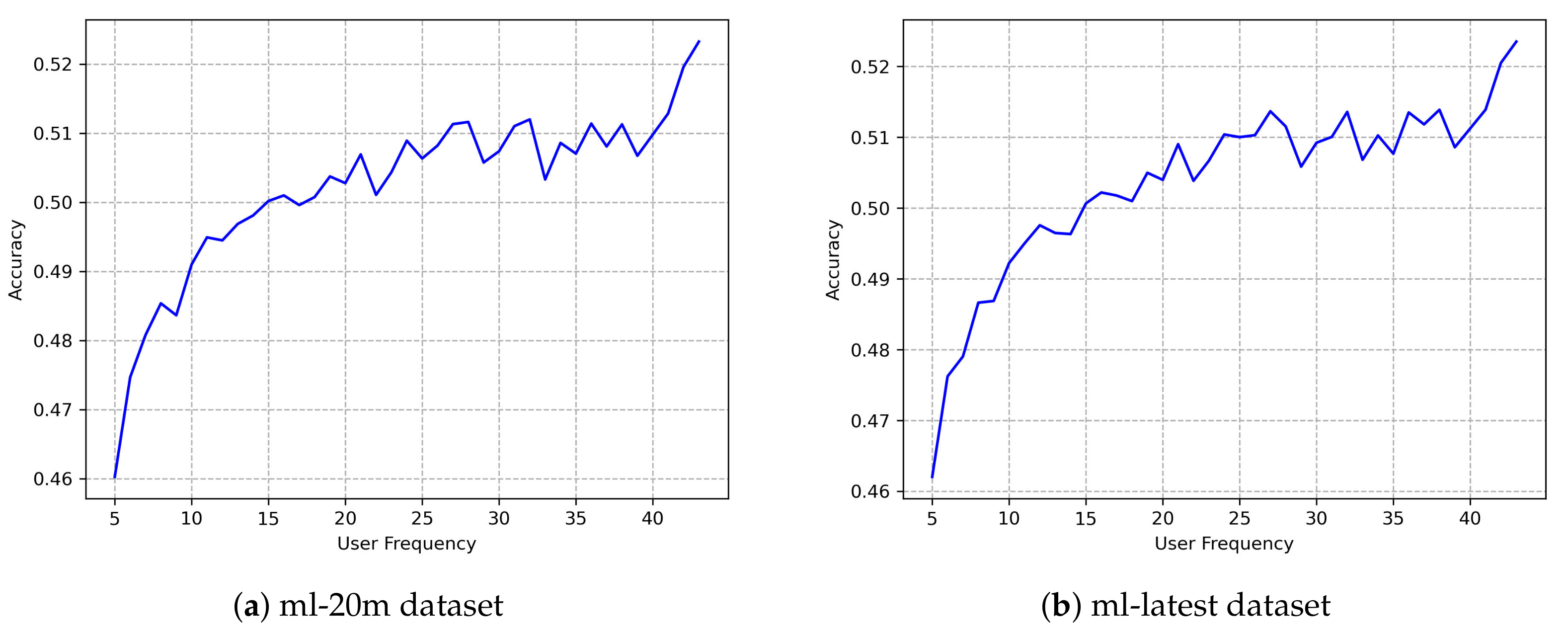
However, although the recommendation accuracy is relatively high when dealing with large datasets, the overfitting phenomenon happens when deep learning models are capturing linear relationships between users and items with reduced dataset sizes [4,5]. Figure 1 shows the prediction accuracy of the Embedding Size Adjustment Policy Network (ESAPN) [4] for users with different frequencies, where the ordinate represents the model’s prediction accuracy and the abscissa represents the user’s frequency. This model is selected as the comparison target in the following section, so the experimental acquisition process of the data in the figure will be introduced later. The model dynamically adjusts the embedding size for user–item feature pairs according to frequency, trying to address the problem of overfitting caused by high-dimensional embedding when dealing with low-frequency datasets. However, it can be found in the figure that a low frequency of user–item interactions corresponds to a lower prediction accuracy in the model, and there still exists a certain degree of overfitting. The reason for this phenomenon is that the deep learning model contains a large number of parameters and requires large amounts of data for training to learn a linear function [6,7]. Low user–item frequency makes it difficult for the model to capture linear relationships between users and items and in turn affects the prediction accuracy. It further illustrates that the linear relationship of the model has a significant impact on the recommendation accuracy. Therefore, in addition to the method of dynamically changing the embedding dimension proposed by the ESAPN model, the overfitting phenomenon can be further alleviated by strengthening the capture of linear relationships, thus improving the prediction accuracy of the model as a whole.
Linear capture technology can improve the performance of deep learning models in capturing linear relationships. Guo et al. [8] designed a neural network model based on a Factorization Machine (FM), in which a multi-layer perceptron was introduced to capture the implicit higher-order interactions between features. In this model, FM was used to capture the second-order linear interactions between feature domains, which improved the overall effect of the model. Since capturing higher-order linear interactions requires a large number of parameters, Wang et al., inspired by residual network [9], proposed a Deep and Cross Network (DCN) model [3], in which a multi-layer perceptron was used to capture implicit higher-order interactions between features. Meanwhile, they used the cross network to capture higher-order linear interactions, improving the linear capture capability of the model. Cheng et al. [2] proposed the Wide and Deep model, which applies the multi-layer perceptron to learn deeper user–item information to recommend more diverse items and uses linear functions to capture the linear relationships between users and items, so as to recommend more related items.
However, these works were all relying on fixed embedding vectors. They did not incorporate multi-dimensional embedding into the model and still used high-dimensional embeddings for low-frequency data. It would make the model prone to overfitting for low-frequency users, thus preventing the model from capturing linear user–item relationships.
In summary, in order to better solve the phenomenon of low frequency data overfitting, to allow the deep learning model to capture linear relationships, and to address defects such as being incapable of integrating the multi-dimensional embedding, this paper proposes the Two-layer Matrix Factorization and Multi-layer Perception Neural Network (TMMNN). In our model, the dimension of the embedding vectors is adjusted according to the data frequency in the adjustment layer to form multi-dimensional embedding vectors. Matrix factorization is introduced as a linear model that linearly combines the latent features of the input data. The neural network of the multilayer perceptron is used to perform in-depth learning of low-dimensional dense embedding vectors and to generalize the unknown features in a low-dimensional way to improve the generalization characteristics of the model. Hence, this model can receive embeddings of different dimensions and capture nonlinear interactions between users and items through the powerful nonlinear fitting ability of the multi-layer perceptron. Moreover, the model can use the linear function of matrix factorization to capture linear user–item relationships.
Compared with the ESAPN model, the advantage of our model lies in the introduction of a linear capture technique—matrix factorization, which is applied especially to capture linear relationships. Our model combines matrix factorization with the dynamic dimension adjustment technology of an embedding vector. Thus, the problem of overfitting in the low-frequency data area can be further solved, and the model’s recommendation efficiency with middle- and high-frequency data can be improved at the same time. Compared with models such as DCN and Wide and Deep, our model has some advantages as well. In our model, the embedding dynamic adjustment technology is introduced, which can dynamically process the input data with changing frequency. This technology is conducive to the capture of linear relationships, and can optimize the memory while improving the recommendation performance of the model for low-frequency data.
In this paper, Section 2 reviews the related research work; Section 3 details the structure and implementation of the TMMNN model; Section 4 discusses the experimental design of the TMMNN model on two evaluation indicators, together with the analysis and discussion of the experimental results; and Section 5 gives the conclusions and future work.
2. Related Work
Capturing linear relationships between users and items is important to the performance of recommender system models [10,11,12]. Traditional matrix factorization techniques can capture the first-order linear relationships using self interaction functions. However, in practical situations, there often exits second-order or higher-order linear relationships between users and items. Rendle et al. [13] proposed a model using Factorization Machine (FM) to capture the first-order and second-order linear relationships between users and items; thus, the model’s ability to capture linear relationships has been improved. Juan et al. [14] found that different feature domains of users and items exhibit heterogeneity when interacting, which hinders the linear capture ability of the model. Therefore they proposed the Field-Aware Factorization Machines (FFMs) model, which stores several embeddings for one feature field. The corresponding embeddings are selected according to interacting objects in the feature domain, which improves the effect of the model. However, it is not enough to rely solely on linear features to output recommender system feedback. The categories of data input to the recommender system are diverse and discrete, forming a huge sparse matrix [3]. New methods are needed to jointly capture the linear and nonlinear features of the data space.
In recent years, because of powerful nonlinear fitting and feature representation capabilities, deep learning has been gradually introduced into recommender systems [15,16]. It is not enough to rely only on nonlinear relationship mining, so many scholars have tried to combine deep learning with linear models. In order to enable the model to capture high-order linear interactions, Wang et al. [3] proposed the Deep Cross Network (DCN) model, which uses a multi-layer perceptron to capture the higher-order implicit interactions between features. The higher-order linear interactions are captured by repeatedly sending the original embedding vectors into the cross network for calculation, which can effectively reduce the model parameters and achieve a high accuracy rate. Cheng et al. [2] proposed the Wide and Deep model, which uses a multi-layer perceptron to learn deeper user information to recommend more diverse items. However, due to limited interactions between users and items, large amounts of irrelevant items were recommended by the model. In that case, a linear model was introduced to capture the linear relationships, so that more related items could be recommended, and the overall accuracy of the model improved. Since the pure DNN network cannot capture the relationships between different feature fields, Qu et al. [17] proposed the Product-base Neural Network (PNN) model, which is the first model using the embedding technology to convert the high-dimensional input into a low-dimensional dense embedding, and then input it into the product layer to capture the interactions between different features of the input data, extract their linear and nonlinear interactions, and finally input them into the subsequent multi-layer perceptron for further extraction of the higher-order interactions.
To summarize, since deep learning contains a large number of parameters, a large amount of training is required to learn any interaction function, which makes it difficult for models to capture linear relationships between users and items with only deep learning. Consequently, overfitting easily occur in the low-frequency data region. When the user’s historical evaluation information is not enough, it is difficult for the recommendation system to accurately grasp the user’s preferences. At the same time, although the above-mentioned DCN, DNN, and other models introduce linear models to make up for the insufficiency of deep learning, they cannot dynamically adjust the dimensions of their embedding vectors. Using high-dimensional embedding in scenarios with small data volumes is still prone to overfitting, which hinders the capture of linear relationships.
There have been many studies combining dynamic embedding vectors with deep learning. The DARTS model [18] proposed by Liu et al. uses a soft selection embedding vector dimension search technique. The AutoEmb model [19] proposed by Zhao et al. is improved on the basis of DARTS. The final embedding dimension is determined by the weighted sum of six fixed-size embedded vectors, and the weight is determined by the frequency of user–item interactions. The ESAPN model [4] uses the hard selection method to realize the embedding vector dimension search technology, which is a further improvement of the above two models. However, these models focus on dynamic embedding, ignoring the capture of linear relationships, and do not employ additional linear models to compensate for the insufficiency of deep learning in low-frequency data regions.
Therefore, it is necessary to construct a new model to strengthen the capture of linear relationships while capturing nonlinear relationships, which introduces dynamic embedding technology to improve the overall accuracy of the recommender system at the same time. In this paper, we propose the TMMNN model based on the ESPAN model. In order to solve the problem of high-dimensional embedding of low-frequency data in deep learning, a method of dynamically adjusting the dimensions of the embedding vectors is used in the model. In order to strengthen the capture of linear relationships between users and items, the matrix factorization method is used in the model, which has the advantages of feeding back implicit information, reacting time effects, etc. [10]. To capture the nonlinear relationships, a multi-layer perceptron is used in the model for in-depth learning.
3. The TMMNN
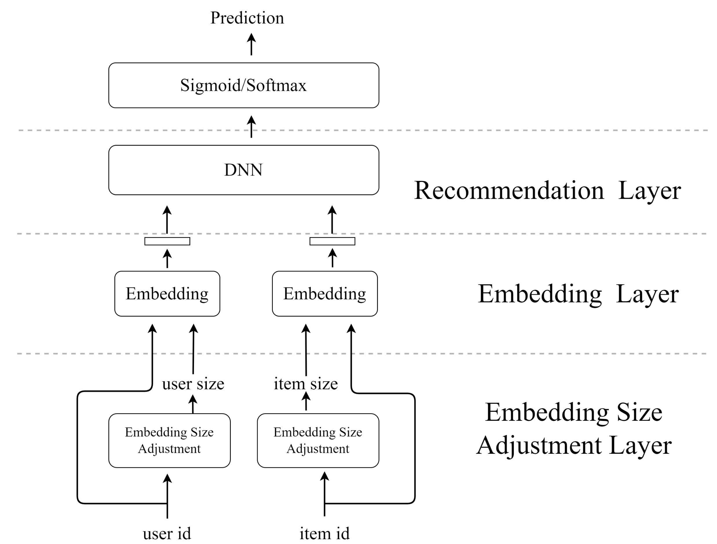
The overall structure of the neural network model, based on two-layer matrix factorization and a multi-layer perceptron, is shown in Figure 2, which consists of three layers: the embedding size adjustment layer, the embedding layer, and the recommendation layer. First, in the TMMNN model, for a given sample label pair, the embedding dimension adjustment layer adjusts the embedding dimensions of users and items, and outputs the adjusted sizes; then, the embedding layer will receive user and item numbers, together with the embedding vector dimensions, and output the corresponding embedding vectors; finally, the embeddings output by the embedding layer are sent to the recommendation layer, and the prediction result is obtained after the calculation by matrix factorization and multi-layer perceptron. The details of each layer will be described in the following sections.
3.1. Embedding Size Adjustment Layer
The embedding size adjustment layer saves the current embedding size and user–item frequency. When receiving a user or item, this layer converts the occurrence frequency of the user or item and the current embedding dimension into the embedding vector and one-hot encoding, respectively. Then, the layer concatenates them and feeds them into the multi-layer perceptron. Through the softmax activation function, the adjustment strategy, i.e., whether the embedding vector is expanded or maintained, is confirmed. Finally, the layer sets the dimension size of the embedding vector as the output. The process is described in detail below.
First, define the state , which contains the user and item occurrence frequency f and the current embedding dimension e. The embedding adjustment layer determines how to adjust the embedding vector size of users and items through the two most basic pieces of information: f and e. Then, it should be noted that the model contains two embedding dimension adjustment layers with the same structure for users and items, respectively. For brevity, in the following part, we take the user’s embedding dimension adjustment layer as an example for introduction.
In order to determine the user’s current state, the embedding dimension adjustment layer needs to obtain the user’s appearance frequency and the current user’s embedding dimension. Considering that the network cannot directly handle integer values, the user frequency f of integer values needs to be converted into the embedding , and the current user embedding size e needs to be converted into a one-hot encoding with dimension n, where n represents the number of candidate embedding size. By concatenating the two elements mentioned above, the embedding z is obtained from the specific equation, which is shown in Equation (1):
In order to determine adjustment policy, the embedding dimension adjustment layer needs to analyze the current user state. Therefore, the spliced embedding z is sent to the multi-layer perceptron for calculation, and finally, the adjustment policy is obtained with the softmax activation function. There are two adjustment options: enlarge or keep it unchanged. Enlarging means that the user’s embedding dimension needs to be expanded from to , while keeping it unchanged means maintaining the user’s current embedding dimension.
3.2. Embedding Layer
The embedding layer consists of two parts, namely, the embedding table and the linear transformation layer. For the conciseness of description, the following introduction is mainly from the perspective of the user’s embedding vector. First, given a user id and user embedding dimension d, the embedding layer will obtain the corresponding user embedding e from the embedding table according to the user embedding dimension d. Then, the layer will send the vector e to the linear transformation layer. The output is a normalized embedding. The process is described in detail as below.
Suppose the user embedding has n candidate dimensions . Suppose there is a user u, and the user embedding e with dimension d is obtained through the embedding adjustment layer and the embedding table. Since the size of the embedding received by the recommendation layer is fixed, the embedding layer needs to send e into the linear transformation layer to obtain an embedding with uniform size. The specific process of linear transformation is shown in Equation (2):
refers to the embedding vector of the n layer. and refers to the transition of trainable weight and bias parameters from n to layers, respectively.
3.3. Recommendation Layer
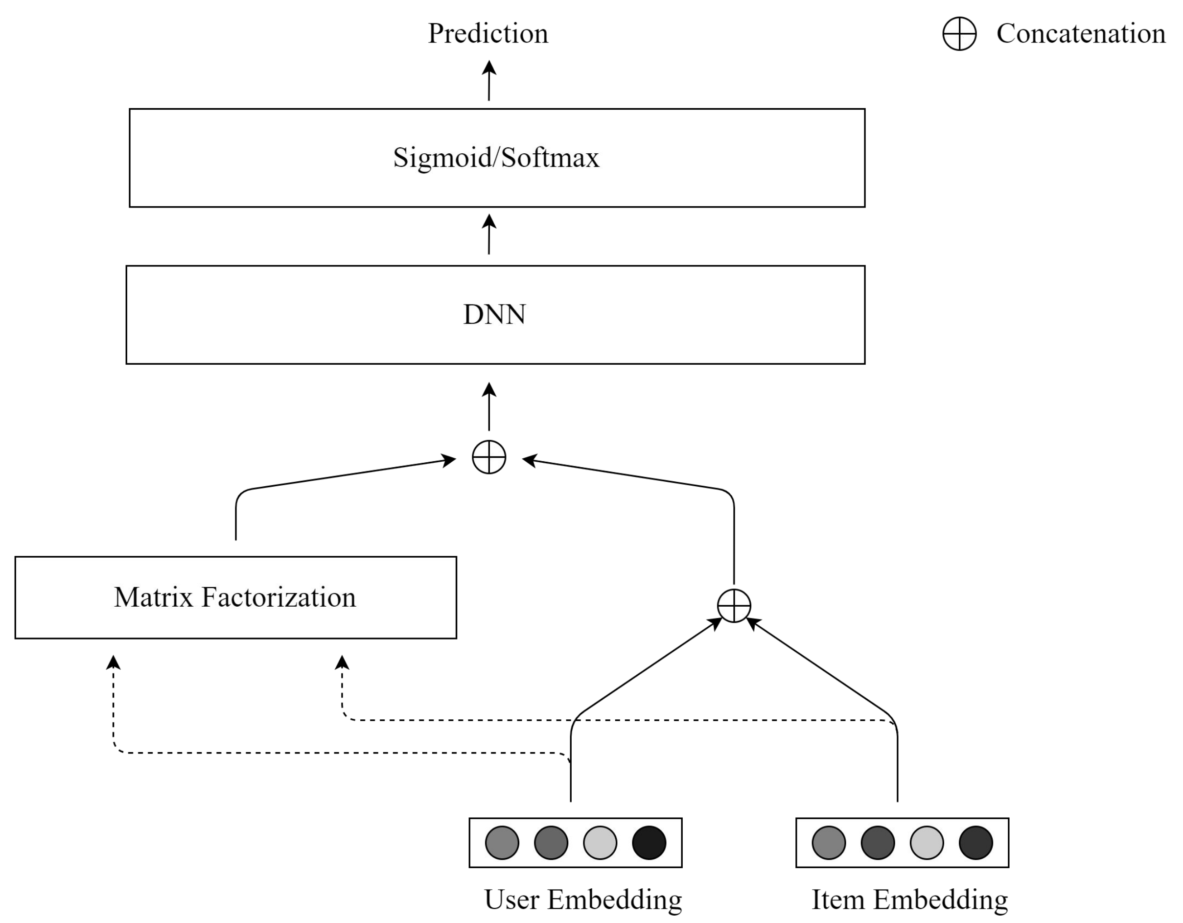
As shown in Figure 3, the recommendation layer consists of two parts: matrix factorization and a multi-layer perceptron. Starting from the bottom of the structure in Figure 3, this layer is fed with the user and item embedding vectors. These two types of embedding vectors can be decomposed in the feature cross layer along the left path. They can be directly spliced along the right path as well. Finally, the results of the above two paths are spliced, and the final prediction is obtained after judgment by the activation function.
In the traditional methods, the model will send embeddings with different dimensions for the matrix factorization and the multi-layer perceptron [20]. However, in the scenario of multi-dimensional embedding, it is difficult for the model to adjust the embedding dimensions for the two components separately, so in this paper, we use two-layer matrix factorization and a multi-layer perceptron to integrate multi-dimensional embedding technology into the model. First, the recommendation layer receives normalized embedding from the user and item embedding layers, labeled and , respectively. Then, our model feeds these two normalized embeddings into matrix factorization to obtain the vector according to Equation (3):
is the weight of the corresponding position, and ⊙ is the bit-wise multiplication. Then, in order to retain the original features of users and items, the embedding is spliced with the embedding and of users and items, and sent to the multi-layer perceptron. The specific process is shown in Equation (4):
⊕ is the connection operation, represents the activation function, and and are trainable weight and bias parameters, respectively. The of the last layer will be fed into the activation function, and the activation function will be selected according to different tasks. For the binary classification tasks and multi-classification tasks introduced in the following section, the model applies the Sigmoid function and the Softmax function, respectively.
4. Experiments
4.1. Datasets
Our model will be tested on two classical benchmark datasets. One of the datasets is the MoveLens 20M Dataset [21], which has a high user–item interaction frequency and thus can test the model’s recommendation accuracy for medium- and high-frequency data. The other dataset is the MovieLens Latest Datasets, which contains more low-frequency user–item interaction data. This dataset can better test the model’s recommendation accuracy for low-frequency data. Next, we will introduce these two datasets:
MovieLens 20M Dataset (ml-20m) [21]: A movie rating dataset collected from the personalized movie recommendation website MovieLens4. The dataset contains 20 million 5-star ratings and 465,000 free-text tags applied to 27,278 movies provided by 138,493 users. These users are randomly selected to ensure every selected user has rated at least 20 movies.
MovieLens Latest Datasets (ml-latest) [21]: A newly released movie rating dataset collected from the same website. The dataset contains 27 million 5-star ratings and 1.1 million tags applied to 58,098 movies from 283,228 users. In this dataset, the users are also randomly selected, and each selected users has rated at least least one movie.
In order to prove our model’s effectiveness, we purposefully divided the above datasets into different sizes, so that the multi-layer perceptron could not learn a linear function due to the lack of training data. Therefore, the model gives full play to the role of matrix factorization to capture the linear relationships to verify the effectiveness of our method.
4.2. Parameters
We set 6 candidate embeddings with dimensions for users and items. We use Adam [22] to optimize the policy network and recommendation model with learning rates set to 0.0001 and 0.003, respectively. The number of dimensions of the fixed embedding is 8. The whole framework is trained on mini-batches with a size of 500. The number of layers of the multi-layer perceptron is set to 1.
We split the dataset into five different sizes, which are 25%, 37.5%, 50%, 62.5%, and 75% of the original size, respectively. Our purpose is to test the influence of dataset size on the prediction results of the model. The smaller the size of the dataset, the greater the ability of the matrix factorization to capture linear relationships, allowing us to examine the overall inhibition degree of the model to the phenomenon of overfitting. This paper only uses two datasets for testing and analysis. However, since the two datasets are divided into different scales during our tests, the impact of our model on prediction results in various situations is essentially considered. The workload in the following testing and evaluation sections is relatively sufficient.
4.3. Tasks and Evaluation Metrics
We evaluated the baselines and our model on a binary classification task and a multi-class classification task.
Binary Classification Task: We transformed the 5-star ratings to binary labels, where ratings of 4 and 5 are viewed as positive while the rest are viewed as negative, and demanded the recommendation model to predict the correct label. We used predictive probability 0.5 as the threshold to assign the label. We measured the performance of the models by the classification accuracy and the mean squared error (MSE) loss. Classification accuracy was acquired by calculating the percentage of the correct prediction number to the total prediction number. The MSE loss can be represented by Equation (5):
Here, is used to parameterize the deep recommendation model. Suppose N pairs of the input user–item data can be represented by ; then, represents the corresponding ground truth label, whose value can be 0 or 1. represents the probability of label to be 1, which is predicted by the recommendation model.
Multi-Classification Task: We viewed the 5-star ratings as 5 classes and made the model predict the correct ratings. In this task, we evaluated the model according to the classification accuracy and the cross-entropy (CE) loss. The calculation method of the classification accuracy is the same as that described in the Binary Task section, and the CE loss value can be represented by Equation (6):
where N represents the mini-batch data’s size, and M represents the number of data classes. represents the ground truth label which shows whether one pair of the data belongs to class m. Similar to , shows the probability that the data belong to class m.
The test difficulty of the binary classification task is relatively small, and the tolerance for the prediction error of the model is relatively large. During this task, the prediction accuracy of the model for a single evaluation is investigated. The multi-classification task requires our model to capture the implicit relationships in user–item interactions, and the capture of nonlinear and linear relationships is more demanding. By carrying out tasks one by one and improving the requirements step by step, the performance of our model for single tasks and complex tasks can be tested more intuitively.
4.4. Baselines
We compared our proposed framework with the following four baseline methods:
Fixed Word Embedding Vector Model (FIXED) [4]: the original recommendation model with embeddings of uniform and fixed sizes. We adopted the embedding size of 128 for all the users and items.
Differentiable Architecture Search (DARTS) [18]: the traditional DARTS method that adjusts embedding sizes by learning the weights for the six candidate embedding sizes for each user or item. The embedding of a user or an item is represented as the weighted sum of the embeddings of the six candidate sizes.
AutoML-based end-to-end framework (AutoEmb) [19]: a DARTS-based method that trains a controller to dynamically assign weights for the six candidate embedding sizes based on the frequency of a given user or item. The embeddings are also represented by soft selection.
Embedding Size Adjustment Policy Network (ESAPN) [4]: this model determines the dimension size of the embedding based on the frequency of items and users. Its policy network is responsible for selecting the embedding size of the user or item embedding. The recommendation layer is responsible for accepting the input and making predictions and finally updating the policy with the activation function. It uses a hard selection method to implement the embedding size search technology and uses the multi-layer perceptron technology to capture the feature relationships between users and items.
Among them, the FIXED model does not use multi-dimensional embedding vectors and linear models such as matrix factorization. The other three models use multi-dimensional embedding vectors but do not introduce linear models. Therefore, in the following section, the TMMNN model proposed in this paper will be compared with these four models so that the overall performance of the two-layer structure can be examined. Moreover, the ESAPN is also the comparison target of the TMMNN model under a small data volume or a low-frequency data area to verify the effect of introducing matrix factorization.
The experimental data and analysis results presented in the following sections are based on the model’s sufficient learning of the given data to predict user behavior. The two datasets with different frequency distributions are divided according to size and frequency. As a result, the model’s performance in various application scenarios is tested, which can reflect the generalization ability of the model to the data, so no new dataset for testing will be introduced in this paper.
4.5. Overall Performance Comparison
Table 1 list the overall performance of all models on the MovieLen 20M and MovieLen Latest datasets. This includes the pure multi-layer perceptron models and the two-layer matrix factorization and multi-layer perceptron model. We use the accuracy and MSE loss as the metrics for the binary classification task and use accuracy and CE loss for the multi-classification task. We bold the test results of the TMMNN model to show the difference.
From the results in the tables, we can draw the following conclusions:
- In this paper, the accuracy of our model on all datasets and all tasks far exceeds that of the fixed model, and our model has a lower loss value as well. Meanwhile, compared to the fixed model, each multi-size embedding model on any dataset and any task has a higher accuracy and a lower loss value. The above conclusion shows that multi-size embedding can improve the performance of the model.
- In terms of accuracy, the model in this paper exceeds all models on all datasets and all tasks, and our model also has the lowest loss value, which indicates that the added matrix factorization technique can improve model performance through the capture of linear interactions.
- The improvement effect of the TMMNN on the ml-latest dataset is not as high as that on the ml-20m. The reason for this difference is that ml-latest can provide more data for the training of the multi-layer perceptron, which further indicates that when the amount of data is insufficient, the linear capture technology can really provide linear capture capability for deep learning models.
- The test results show that our model improves the prediction accuracy in both binary classification and multi-classification tasks. Although the performance improvement in two tasks is numerically similar, the performance on the multi-classification task is better with smaller benchmark values. This shows that in the face of complex evaluation indicators, the simultaneous introduction of linear models and multi-dimensional embedding vectors plays a significant role in capturing implicit interactions.
4.6. Analysis of the Performance in Small Data Volumes
The introduction of matrix factorization can provide linear capture capability to the model. In order to investigate whether matrix factorization can help to improve the performance of the model in scenarios with small data volumes, we used the method of clipping on the basis of the two datasets, namely, MovieLens 20M and MovieLens Latest, to divide a number of small datasets. The database was cut according to the proportions of 25%, 37.5%, 50%, 62.5%, and 75%, and then training was performed on the datasets that have been cut. By varying the dataset size and task types, we simulated 10 different scenarios for each of the two datasets. For the ml-latest dataset with more low-frequency data, the results can reflect the impact of prediction accuracy under low-frequency interactions, and the experiments can fully test our model’s mitigation effect on overfitting. The ml-20m dataset, which mainly contains medium- and high-frequency data, is used to check whether the model can maintain the prediction accuracy in general, except in the special case of low-frequency small datasets. In this subsection, the experiment only changes the size of the two datasets so as to study the effect of dataset size on the linear capture ability of our model.
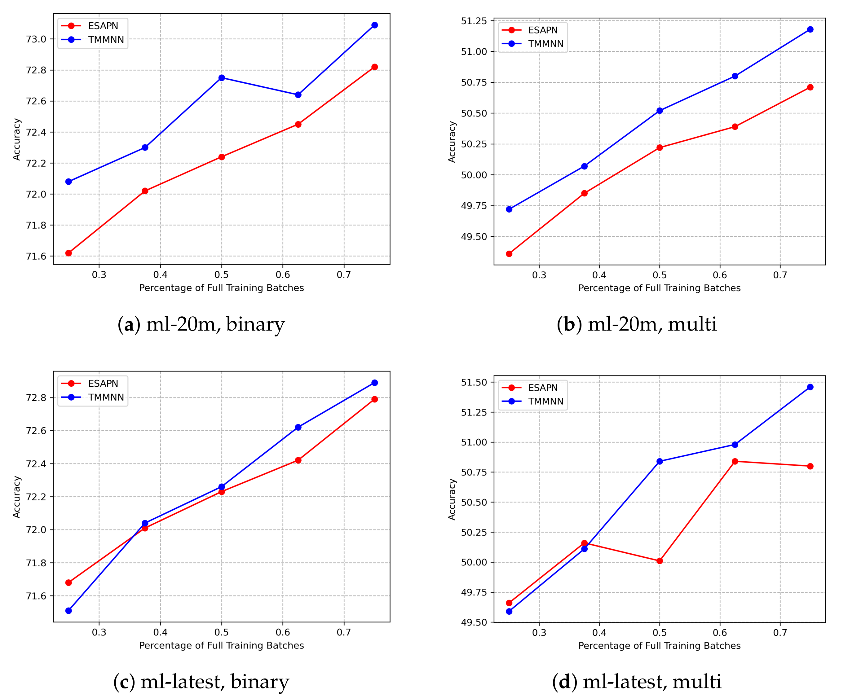
Figure 4 shows the accuracy of the ESAPN and TMMNN on various datasets and tasks; the red line represents ESAPN, and the blue line represents TMMNN. The abscissa shows the percentage of full training batches. The original data set is randomly cropped by a percentage to serve as the training set, and the interaction information of the same user is selected as the test set in the remaining data. Combining the two datasets and the two classification tasks yields four different situations, which are shown separately in four subplots. The following conclusions can be drawn from the figure:
- (1)
- Our model outperforms the ESAPN on all datasets and all tasks, which shows that the addition of matrix factorization can indeed improve the effectiveness of the model.
- (2)
- The model shows more improvement in ml-20m than in ml-latest. Considering that the amount of data the former dataset has is much smaller than that of the latter, this phenomenon can also be interpreted as the matrix factorization improving the model more significantly in a small amount of data.
- (3)
- It can be seen from the figure that when the size of the training dataset gradually increases, the performance of the TMMNN does not lag behind. This can be explained by the fact that as the amount of data increases, the multi-layer perceptron is gradually affected by the sufficient training, so the accuracy of the model can be guaranteed to continue to increase.
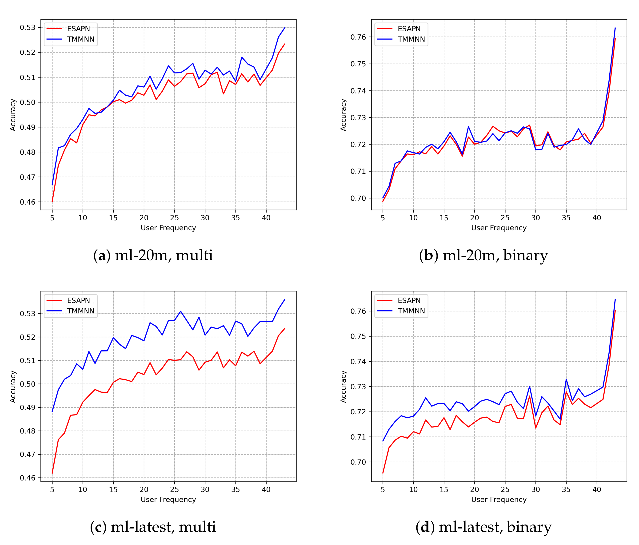
4.7. Analysis of the Low-Frequency Users
In order to further explore whether the model can capture linear interactions after adding matrix factorization to the model, we conducted experiments on binary classification and multi-classification tasks on the ml-20m and ml-latest datasets, respectively, so as to improve the overall effectiveness of the model. During the experiment of this subsection, we divided the datasets according to the frequency of user–item interactions, studied our model’s performance from the perspective of frequency, and focused analysis on the prediction accuracy for low-frequency data. The comparison model for this experiment is the ESAPN, which is a deep learning model based on multi-size embedding. The experimental results are shown in Figure 5. The ordinal number in the graph shows the prediction accuracy, and the horizontal coordinate represents the occurrence frequency of users. The specific meaning is explained as follows: We divided the frequency of user appearance into 43 frequency categories, and each category represents a set of frequencies. Category 41 means that the user appears 200 to 500 times, Category 42 indicates that the user appears 500 to 1000 times, and Category 43 indicates that the user appears more than 1000 times. The frequency intervals of the remaining categories can be calculated according to Equation (7):
In Equation (7), F represents the frequency of the user, and k represents the frequency category of the user. Therefore, the value range of the abscissa user frequency is , and each value represents a numerical interval of user frequency. Based on the original datasets, all interaction data in this interval are screened out. All interactions of the same user are randomly divided into a training set and test set, and the obtained accuracy on the test set is taken as the numerical result of the ordinate.
It is evident that, compared to the MovieLen 20M dataset, on which matrix factorization has slight positive influences, the MovieLens Latest dataset has been significantly improved in all tasks. Since the former dataset mainly consists of medium- and high-frequency data and the latter consists of more low-frequency data, the matrix factorization method has a more obvious impact on improving the prediction accuracy of low-frequency data. Moreover, the effect of TMMNN is much better than ESAPN, and we can notice that the blue curves in Figure 5c,d are much higher than the red curves in the low frequency data area, which indicates that the addition of matrix factorization can actually help the model to capture the linear interactions and improve the prediction accuracy of low-frequency users. Hence, the result proves the effectiveness of the method.
5. Conclusions
Due to the fixed dimension of the embedding vector, the deep learning models embed high-dimensional vectors in the low-frequency region, which is prone to overfitting. In the meantime, the models contain a huge number of parameters and require a lot of training data to learn linear functions that capture linear interactions, making it difficult for models to capture linear relationships. To address this problem, this paper proposes a neural network model using two-layer matrix factorization and a multi-layer perceptron (TMMNN), which embeds multi-dimensional vectors with dynamic adjustments, uses the linear function of matrix factorization to allow the model to capture the linear relationships between users and items, and uses the multi-layer perceptron to capture the nonlinear relationships at the same time. The experimental results on a large amount of real data in the datasets show that the performance of the TMMNN under a small data volume has increased, and the prediction accuracy of low-frequency users has been improved. The effectiveness and feasibility of the TMMNN have thus been verified. Therefore, the establishment of this model can improve the accuracy of service recommendation, help the predictive delivery of network services, and further improve user experience.
In the future, it can be further optimized from two directions of linear model and multi-dimensional embedding. For linear models, we can innovate on the basis of matrix factorization to try to capture linear interactions above the second order. For multi-dimensional embedding, there is still room for development based on the hard selection method, and further improving the dynamics of the embedding vectors is one of the goals of future development.
Author Contributions
S.B.: Conceptualization (equal), methodology (equal), software (equal); T.W.: methodology (equal), data curation, writing—original draft preparation; L.Z.: software (equal), visualization, investigation (equal); G.D.: conceptualization (equal), investigation (equal); G.S.: supervision, writing—reviewing and editing (equal); J.S.: validation, writing—reviewing and editing (equal); All authors have read and agreed to the published version of the manuscript.
Funding
This research received no external funding.
Institutional Review Board Statement
Not applicable.
Informed Consent Statement
Not applicable.
Data Availability Statement
Not applicable.
Conflicts of Interest
The authors declare no conflict of interest.
References
- Zhang, S.; Yao, L.; Sun, A.; Tay, Y. Deep learning based recommender system: A survey and new perspectives. ACM Comput. Surv. (CSUR) 2019, 52, 1–38. [Google Scholar] [CrossRef] [Green Version]
- Cheng, H.T.; Koc, L.; Harmsen, J.; Shaked, T.; Chandra, T.; Aradhye, H.; Anderson, G.; Corrado, G.; Chai, W.; Ispir, M.; et al. Wide and deep learning for recommender systems. In Proceedings of the 1st Workshop on Deep Learning for Recommender Systems, Boston, MA, USA, 15 September 2016; pp. 7–10. [Google Scholar]
- Wang, R.; Fu, B.; Fu, G.; Wang, M. Deep and cross network for ad click predictions. In Proceedings of the ADKDD’17, Halifax, NS, Canada, 13–17 August 2017; pp. 1–7. [Google Scholar]
- Liu, H.; Zhao, X.; Wang, C.; Liu, X.; Tang, J. Automated embedding size search in deep recommender systems. In Proceedings of the 43rd International ACM SIGIR Conference on Research and Development in Information Retrieval, Online, 25–30 July 2020; pp. 2307–2316. [Google Scholar]
- Liu, B.; Tang, R.; Chen, Y.; Yu, J.; Guo, H.; Zhang, Y. Feature generation by convolutional neural network for click-through rate prediction. In Proceedings of the World Wide Web Conference, San Francisco, CA, USA, 13–17 May 2019; pp. 1119–1129. [Google Scholar]
- Rendle, S.; Krichene, W.; Zhang, L.; Anderson, J. Neural collaborative filtering vs. matrix factorization revisited. In Proceedings of the Fourteenth ACM Conference on Recommender Systems, Online, 22–26 September 2020; pp. 240–248. [Google Scholar]
- Andoni, A.; Panigrahy, R.; Valiant, G.; Zhang, L. Learning polynomials with neural networks. In Proceedings of the International Conference on Machine Learning, Beijing, China, 21–26 June 2014; pp. 1908–1916. [Google Scholar]
- Guo, H.; Tang, R.; Ye, Y.; Li, Z.; He, X. DeepFM: A factorization-machine based neural network for CTR prediction. arXiv 2017, arXiv:1703.04247. [Google Scholar]
- He, K.; Zhang, X.; Ren, S.; Sun, J. Deep residual learning for image recognition. In Proceedings of the Proceedings of the IEEE Conference on Computer Vision and Pattern Recognition, Las Vegas, NV, USA, 27–30 June 2016; pp. 770–778.
- Koren, Y.; Bell, R.; Volinsky, C. Matrix factorization techniques for recommender systems. Computer 2009, 42, 30–37. [Google Scholar] [CrossRef]
- Jin, R.; Li, D.; Gao, J.; Liu, Z.; Chen, L.; Zhou, Y. Towards a better understanding of linear models for recommendation. In Proceedings of the 27th ACM SIGKDD Conference on Knowledge Discovery and Data Mining, Online, 14–18 August 2021; pp. 776–785. [Google Scholar]
- Steck, H. Embarrassingly shallow autoencoders for sparse data. In Proceedings of the World Wide Web Conference, San Francisco, CA, USA, 13–17 May 2019; pp. 3251–3257. [Google Scholar]
- Rendle, S. Factorization machines. In Proceedings of the 2010 IEEE International Conference on Data Mining, Sydney, Australia, 13–17 December 2010; pp. 995–1000. [Google Scholar]
- Juan, Y.; Zhuang, Y.; Chin, W.S.; Lin, C.J. Field-aware factorization machines for CTR prediction. In Proceedings of the 10th ACM Conference on Recommender Systems, Boston, MA, USA, 15–19 September 2016; pp. 43–50. [Google Scholar]
- Lian, J.; Zhou, X.; Zhang, F.; Chen, Z.; Xie, X.; Sun, G. xdeepfm: Combining explicit and implicit feature interactions for recommender systems. In Proceedings of the 24th ACM SIGKDD International Conference on Knowledge Discovery and Data Mining, London, UK, 19–23 August 2018; pp. 1754–1763. [Google Scholar]
- Elkahky, A.M.; Song, Y.; He, X. A multi-view deep learning approach for cross domain user modeling in recommendation systems. In Proceedings of the 24th International Conference on World Wide Web, Florence, Italy, 18–22 May 2015; pp. 278–288. [Google Scholar]
- Qu, Y.; Cai, H.; Ren, K.; Zhang, W.; Yu, Y.; Wen, Y.; Wang, J. Product-based neural networks for user response prediction. In Proceedings of the 2016 IEEE 16th International Conference on Data Mining (ICDM), Barcelona, Spain, 12–15 December 2016; pp. 1149–1154. [Google Scholar]
- Liu, H.; Simonyan, K.; Yang, Y. Darts: Differentiable architecture search. arXiv 2018, arXiv:1806.09055. [Google Scholar]
- Zhao, X.; Liu, H.; Fan, W.; Liu, H.; Tang, J.; Wang, C.; Chen, M.; Zheng, X.; Liu, X.; Yang, X. AutoEmb: Automated Embedding Dimensionality Search in Streaming Recommendations. In Proceedings of the 2021 IEEE International Conference on Data Mining (ICDM), Auckland, New Zealand, 7–10 December 2021; pp. 896–905. [Google Scholar]
- He, X.; Liao, L.; Zhang, H.; Nie, L.; Hu, X.; Chua, T.S. Neural collaborative filtering. In Proceedings of the 26th International Conference on World Wide Web, Perth, Australia, 3–7 April 2017; pp. 173–182. [Google Scholar]
- Harper, F.M.; Konstan, J.A. The MovieLens Datasets: History and Context. ACM Trans. Interact. Intell. Syst. 2015, 5, 1–19. [Google Scholar] [CrossRef]
- Kingma, D.P.; Ba, J. Adam: A method for stochastic optimization. arXiv 2014, arXiv:1412.6980. [Google Scholar]
Figure 1.
Prediction accuracy of users with different frequencies.

Figure 2.
Overview of the TMMNN.

Figure 3.
Recommendation Layer overview of the TMMNN.

Figure 4.
Testing accuracy based on different percentage of full training batches.

Figure 5.
Testing accuracy based on training batches with different user-item frequencies.


Table 1.
Overall performance comparison on baselines and TMMNN models.
| ml-20m | ||||
| Method | Binary | Multiclass | ||
| Accuracy | MSE Loss | Accuracy | CE Loss | |
| FIXED | 72.13 | 0.1845 | 49.45 | 1.1517 |
| DARTS | 72.18 | 0.1836 | 49.85 | 1.1423 |
| AutoEmb | 72.27 | 0.1828 | 49.94 | 1.1399 |
| ESAPN | 72.98 | 0.1785 | 50.98 | 1.1155 |
| TMMNN | 73.37 | 0.1766 | 51.48 | 1.1101 |
| ml-latest | ||||
| Method | Binary | Multiclass | ||
| Accuracy | MSE Loss | Accuracy | CE Loss | |
| FIXED | 72.13 | 0.1845 | 50.01 | 1.1414 |
| DARTS | 72.22 | 0.1834 | 50.46 | 1.1304 |
| AutoEmb | 72.36 | 0.1823 | 50.47 | 1.1311 |
| ESAPN | 72.88 | 0.1790 | 51.11 | 1.1147 |
| TMMNN | 73.26 | 0.1773 | 51.37 | 1.1072 |
Publisher’s Note: MDPI stays neutral with regard to jurisdictional claims in published maps and institutional affiliations. |
© 2022 by the authors. Licensee MDPI, Basel, Switzerland. This article is an open access article distributed under the terms and conditions of the Creative Commons Attribution (CC BY) license (https://creativecommons.org/licenses/by/4.0/).
Share and Cite
MDPI and ACS Style
Bao, S.; Wang, T.; Zhou, L.; Dai, G.; Sun, G.; Shen, J. Two-Layer Matrix Factorization and Multi-Layer Perceptron for Online Service Recommendation. Appl. Sci. 2022, 12, 7369. https://doi.org/10.3390/app12157369
AMA Style
Bao S, Wang T, Zhou L, Dai G, Sun G, Shen J. Two-Layer Matrix Factorization and Multi-Layer Perceptron for Online Service Recommendation. Applied Sciences. 2022; 12(15):7369. https://doi.org/10.3390/app12157369
Chicago/Turabian StyleBao, Shudi, Tiantian Wang, Liliang Zhou, Guilan Dai, Geng Sun, and Jun Shen. 2022. "Two-Layer Matrix Factorization and Multi-Layer Perceptron for Online Service Recommendation" Applied Sciences 12, no. 15: 7369. https://doi.org/10.3390/app12157369
Note that from the first issue of 2016, this journal uses article numbers instead of page numbers. See further details here.