
A Review of Neural Network-Based Emulation of Guitar Amplifiers
by
 , ,
, ,
Tara Vanhatalo
1,2,3,* ,
,
Pierrick Legrand
1,
Myriam Desainte-Catherine
2,
Pierre Hanna
2,
Antoine Brusco
3,
Guillaume Pille
3 and
Yann Bayle
3 1
Inria Bordeaux Sud-Ouest, Institute of Mathematics of Bordeaux, UMR 5251 CNRS, University of Bordeaux, F-33405 Talence, France
2
University of Bordeaux, CNRS, Bordeaux INP, LaBRI, UMR 5800, F-33400 Talence, France
3
Orosys, F-34980 Saint-Gély-du-Fesc, France
*
Author to whom correspondence should be addressed.
Appl. Sci. 2022, 12(12), 5894; https://doi.org/10.3390/app12125894
Submission received: 26 April 2022
/
Revised: 1 June 2022
/
Accepted: 8 June 2022
/
Published: 9 June 2022
(This article belongs to the Topic Artificial Intelligence Models, Tools and Applications)
Abstract
:Vacuum tube amplifiers present sonic characteristics frequently coveted by musicians, that are often due to the distinct nonlinearities of their circuits, and accurately modelling such effects can be a challenging task. A recent rise in machine learning methods has lead to the ubiquity of neural networks in all fields of study including virtual analog modelling. This has lead to the appearance of a variety of architectures tailored to this task. This article aims to provide an overview of the current state of the research in neural emulation of analog distortion circuits by first presenting preceding methods in the field and then focusing on a complete review of the deep learning landscape that has appeared in recent years, detailing each subclass of available architectures. This is done in order to bring to light future possible avenues of work in this field.
1. Introduction
The use of vacuum tubes in electronics has largely diminished since the advent of semiconductor technologies, leading to their replacement in almost all fields except that of music technology, where a return to and rise of vacuum tubes can be observed [1]. Musicians tend to prefer the sonic characteristics of vacuum tube amplifiers over those of solid-state ones. Nevertheless, the shortcomings of vacuum tubes in the realm of guitar amplification are numerous and include elevated cost and weight, poor durability, and high power consumption. Their solid-state counterparts remedy some of the disadvantages of vacuum tube amplifiers but remain less popular among musicians who often seek the particular tone of the tube amplifiers used in iconic albums and guitar rigs.
Researchers have turned to Digital Signal Processing (DSP) methods for the emulation of vacuum tube amplifiers in order to circumvent some of the downsides of this technology. These DSP methods are not limited to guitar amplification or distortion and can consist of a wide range of audio effects such as reverberation, delay, and pitch-shifting [2]. The existing DSP methods for tube amplifier emulation can be divided into three categories depending on the degree of prior knowledge of the target device used. The “white-box” approach is historically the first and emulates each electronic component. The “black-box” approach tries to match the output of the target device given a specific input using mathematical functions uncorrelated with the internal components. Gray-box methods are similar to black-box but utilize some information about the target device in order to fine-tune the model. They comprise a block-oriented structure inspired by internal information of the device but the simulation disregards the behaviour of each of the individual components. These three modelling approaches will be discussed in further detail in Section 2.
These three “traditional” methods do, however, present some drawbacks. On one end of the spectrum, obtaining the internal knowledge of the target device needed for white-box approaches is both a costly and labour-intensive task and can provide inaccuracies in the emulation. They can also be computationally expensive. On the other side of the spectrum, black-box methods can also be computationally costly or cannot accurately approximate the nonlinear mapping of the amplifier. These methods will be discussed further in a future section. The computational cost of these methods is also prohibitive for real-time use, which is a fundamental factor to be considered in Virtual Analog (VA) modelling. Amplifier emulations need to be fast enough to run in real-time in order to be used by musicians. If the latency of an emulation exceeds around 10 ms, it can be perceived by the musician and hinder their playing [3].
The use of machine learning, in particular neural networks, has seen a significant increase in all data-related fields in recent years due to, in part, the increased computational capabilities of modern-day computers and the possibility of parallelizing computations on their GPU. The field of audio processing is no exception and the application of neural networks to the task of tube amplifier emulation seems to be appropriate. Indeed, neural networks are made up of the basic building blocks necessary for this type of problem including the presence of nonlinear activation functions which are well suited to model the nonlinearities created by vacuum tubes. Moreover, certain neural network architectures are able to capture and replicate the dynamic nature of a system. For example, autoregressive models retain information from previous time steps for their computations. Thus, the memory effect of amplifiers can be modeled using the appropriate type of neural network. Additionally, neural networks reduce the time necessary to create the emulation of a given analog device. Whereas for white- and gray-box methods it is necessary to repeat the modelling process for each circuit, only the training data needs to be modified for a new emulation via neural networks. The architecture remains unchanged. Parallels have also been made between typical DSP filters and certain neural networks [4]. Therefore, neural networks appear to be an appropriate candidate for the task of vacuum tube amplifier emulation.
The goal of this paper is to present an overview of the current state-of-the-art methods in vacuum tube amplifier emulation, with a focus on the newly emerging deep learning (DL) approaches. The structure of this paper is as follows: Firstly, a brief overview of the traditional white-, gray-, and black-box approaches mentioned above will be presented in Section 2; Then, an extensive review of the current neural network architectures used for amplifier emulation will be presented along with an evaluation of the approaches as well as their limitations in Section 3. Finally, a summary and discussion of the architectures will be given with the intent of providing a global view of the state-of-the-art in Section 4.
2. Traditional Methods
2.1. White-Box
The first class of methods used for the emulation of vacuum-tube distortion aims to create a model of the physical device using internal information of the amplifier to establish a system of differential equations. The main methods of this approach are state-space models, Modified Nodal Analysis (MNA), Port-Hamiltonian formalism, and the use of Wave Digital Filters (WDF). Here we present a non-exhaustive list of white-box methods in order to illustrate the limitations that can occur. More detail on the landscape of white-box methods can be found, for example, in the works of Pakarinen and Yeh [5,6].
Nodal analysis is a method used in circuit simulation techniques in order to establish the system of equations in matrix form to be solved. This is accomplished using the Kirchhoff Circuit Laws (KCL) at each node. Modified Nodal Analysis extends this to incorporate auxiliary equations into the system using the circuit’s Branch Constitutive Equations (BCE) in order to solve the resulting system, which has the following form: MV = I where M is the matrix of conductance coefficients for KCL, I is a vector of independent current sources in the circuit, and V is the vector of unknowns (which are typically voltages). The most well-known electronic circuit simulator is SPICE (Simulation Program with Integrated Circuit Emphasis), which uses a combination of component-wise discretization of the circuit and MNA to create the system to be solved. This approach, while accurate, is computationally heavy and therefore poses a problem for real-time use [6]. Moreover, if an element within the circuit is changed, the MNA process needs to be repeated to take into account this change.
The WDF approach constructs digital filters based on the traveling-wave formulation of the physical elements of the device, obtained via a change of variables from the Kirchhoff to the wave domain which describes circuit dynamics in terms of incident waves and reflected waves . Unlike nodal analysis, this formalism allows for modularity without delay-free loops (i.e., loops that cannot be computed as the input and resulting output are needed at the same time step in order to accomplish this). Discrete-time models of each of the individual components (resistors, capacitors, and inductors) are connected to construct the filter. An interesting benefit of this approach is that the finite difference scheme resulting from the use of the bilinear transform for the discretization remains explicit for any number of models. WDF was used to model a number of distortion effects including a triode amplifier in [7].
State-space models rely on the principle that the equations of motion for any physical system may be formulated in terms of the state of the system: where is the state of the system at time t, is a vector of external inputs, and the general vector function specifies how the current state and inputs cause a change in the state at time t. may be time-varying itself. All past states and the entire input history are “summarized” by the current state . Thus, must include all the “memory” of the system.
To solve the nonlinear state space system, two notable approaches are the K-method and the Discrete K-method (DK-method). The K-method was originally proposed to avoid noncomputable delay-free loops in the system. It does this by transforming the system to highlight all loops involving nonlinear maps. The delay-free paths are isolated in order to be eliminated via geometrical transformations [8].
The DK-method establishes a system of Ordinary Differential Equations (ODE) based on MNA which is then solved to find the state transition matrix and the nonlinear relationships between variables in order to produce a nonlinear filter similar to that of the K-method. However, in the K-method, the ODE are discretized after derivation whereas in the DK-method, discretization is applied first [9]. David Yeh applies the DK-method to model a Bipolar-Junction Transistor (BJT) and a triode amplifier in a real-time plugin and evaluates this against a reference SPICE model [9].
The final method that will be described consists of a state-space representation that is structured based on the various energies of a system and their dynamics. This representation is structured into its energy-storing parts, dissipative parts, and then the external sources of energy [10]. This structure falls under the Port-Hamiltonian (PH) formalism. Like for the K-method family of approaches and WDF, the PH structures are derived from the circuit schematic by use of its reigning Kirchhoff laws. However, unlike the other two methods, the passivity property is conserved which ensures stability of the model [10]. This approach has been successfully used for the simulation of such analog effects as a BJT amplifier and a wah pedal in [10].
Each of these methods translates the circuit diagram of a given amplifier into a set of equations that completely describes the system which is then discretized, usually using a finite-difference or integration scheme, to then be solved iteratively. In order to establish these equations, access to the circuit diagram or study of the internal structure of the amplifier is necessary and results in a labour-intensive task. Moreover, the resolution of these differential equations relies on computationally expensive iterative methods or storing lookup tables and the component values measured can also introduce inaccuracies into the emulation or fail to faithfully emulate the particularities of a given amplifier.
2.2. Gray-Box
Gray-box methods seek to alleviate some of the labour required for the modelling task using white-box approaches. They do this by incorporating internal knowledge of the device in the form of blocks in order to simplify the model. Indeed, modelling each of the individual circuit components is not necessary in gray-box; only the behaviour of the device as a whole needs to be modelled.
Block-Oriented structures are a subclass of Volterra series [11] that aim to separate the Device-Under-Test’s (DUT) effect on the input signal into “blocks”: one set dealing with the dynamic, linear behaviour of the system, and one to introduce the nonlinearity. The common configurations of these structures are the following:
- Hammerstein (and their subclass cascade Hammerstein) models: Static nonlinearity followed by linear filter.
- Wiener models: Linear filter followed by static nonlinearity.
- Wiener-Hammerstein models: Static nonlinearity between two linear filters.
Block-Oriented structures can be considered as gray-box methods as they can take into account the high-level structure of the DUT for their configuration and most examples of block-oriented structures applied to distortion approximation fall under the realm of gray-box modelling.
One of these configurations (Wiener–Hammerstein) has even been described as the “fundamental paradigm of electric guitar tone” in [12] and this family of methods is used in commercial products and patents such as Fractal Audio’s Axe-Fx [12] and a 2008 patent from Kemper [13]. This patent describes a Wiener–Hammerstein topology and Fractal’s white paper extends this model to include extra linear and nonlinear blocks in their MIMIC technology. Most notable in the field of gray-box guitar amplifier modelling using block-oriented structures are the works of Felix Eichas and Udo Zölzer, in which system identification using input–output signals and optimization of the block topology using iterative methods to minimize the error between model output and the measured target are used. These approaches will be detailed in this section.
In [14], a parametric Wiener–Hammerstein model for distortion effects is presented along with the iterative algorithm used for the optimization portion of the problem. The Levenberg–Marquardt algorithm was chosen for the minimization and the DUT was a Hughes and Kettner Tube Factor amplifier. This method produced satisfying results that were nearly indistinguishable from the target, but the model becomes more inaccurate for frequencies outside of the range [60 Hz, 18 kHz].
In a following work, an extended Wiener model was tested for the emulation of three different distortion devices: a diode clipper with pre-amplification of the input signal, a BJT distortion stage of an Electro-Harmonix Big Muff Pi, and the op-amp stage of an Ibanez Tube Screamer (all simulated using a SPICE circuit simulator). This simple topology had a harder time modelling the desired effects and only the diode clipper circuit was modeled successfully.
Eichas and Zölzer [15] presented a gray-box approach in which the modelling process is automatic using input–output measurements and iterative optimization. Its structure is the following: three linear filters inter-spaced with nonlinear blocks, the first consisting of a polynomial waveshaping function and the second consisting of a concatenation of hyperbolic tangents. An Exponential Sine Sweep (ESS) is used for the system identification process along with the Levenberg–Marquardt algorithm for the optimization problem. This method was used to model a Fender Bassman 100 and an Ampeg VT-22 but struggled at modelling distortion.
Finally, in [16], analog amplifiers including a Bassman 100 and a JCM 900 were modeled with an automated procedure and an extended Wiener–Hammerstein configuration consisting of a nonlinear mapping between two Linear Time-Invariant (LTI) blocks connected in series. Again the Levenberg–Marquardt was used for the optimization and the model performed well even for strong nonlinearities and has a low computational load compared to white-box methods but is not able to incorporate certain subtle effects such as power sagging or crossover distortion.
Block-oriented, gray-box methods present a lower computational cost than white-box methods but struggle with emulating the target devices more so than the latter class of methods.
In addition to the block-oriented structures presented here, the use of machine learning and Artificial Neural Networks (ANN) has started to see a rise in the gray-box approaches and will be detailed further in a later section.
2.3. Black-Box
Black-box approaches are system identification methods that seek to remedy some of the problems of gray- and white-box approaches by relying on only input–output measurements to describe the overall behaviour of the amplifier. These methods enable emulation without the need for prior knowledge of the internal circuitry of the amplifier. They also tend to be more computationally efficient than white-box models and allow for the replication of idiosyncrasies that can exist in the analogue devices (due to imperfect electrical components for example). The main methods in this category are Volterra series, dynamic convolution, block-oriented structures (which are a subclass of Volterra series), and kernel regression.
Dynamic convolution, proposed in [17], is a variant of the system identification method used for linear systems in which instead of a single impulse response used to derive the transfer function of the DUT, multiple impulses are used as input at different amplitudes in order to obtain an approximation of the nonlinear behaviour. In this work, the standard convolution operation where h is the impulse response of length L, y is the output signal, and x the input, is replaced with so-called dynamic convolution operation defined as follows:
where is a selector function that determines which impulse response should be used for the input sample . This method was used in the Sintefex FX8000 Audio Effects Replicator.
Certain Machine Learning (ML) methods have also been proposed for the emulation of guitar distortion circuits. A Support Vector Machine (SVM), which is a class of linear ML algorithm, was used to emulate a common-cathode tube amplifier via kernel regression [18]. In the article, the authors linearize the nonlinear system in order to be able to apply the SVM to the regression task and suggest methods for choosing the proper kernel to linearize the system. The linearization is accomplished by mapping the data into a higher-dimensional vector space in which the nonlinear functions of the system can be replaced by linear operators. Kernel methods are used to avoid the computationally intensive task of representing these functions in the higher-dimension space, requiring instead only the computation of the inner products between the vectors in this new space. While this method is theoretically solid, the choice of the necessary mappings and kernel function can be a difficult task.
ANN are a class of machine learning, black-box methods that use neurons and nonlinear activation functions such as sigmoid or hyperbolic tangent, functions frequently used in VA modelling to model various nonlinearities. This enables ANN to approximate complex mappings and recent technological improvements have enabled their wide-spread, leading to a rise of artificial intelligence in almost all fields in recent years. Similarities between a number of ANN architectures and certain black-box modelling methods can be drawn and suggest that they would appear to be well suited to the task of vacuum tube amplifier emulation as we shall discuss in further detail in a future section.
The Volterra series [19] is a functional expansion of multidimensional convolution kernels that enables the emulation of the “memory” effect of an amplifier as the output of the nonlinear system is dependent on the input at previous time steps. It is an extension of the common model of a linear system: , where H is the transfer function of the system and the input. It expands this model to include nonlinearities by adding convolution integrals that take into account the interactions between the previous inputs thereby retaining the “memory” effect of the causal system:
The functionals of this expansion, called Volterra kernels, can be estimated using various methods (e.g., cross-correlation or least-squares) but is a computationally intensive task. Moreover, Volterra series work well for relatively linear systems but struggle when the system being modeled exhibits very strong nonlinear behaviour. An example of Volterra series applied to the simulation of analog audio devices is presented in [20] where this method is used to emulate the weakly nonlinear behaviour of the Moog ladder filter. This filter is a key contributing factor to the Moog synthesizer’s sound and is named so because of its schematic that resembles a ladder.
The block-oriented structures presented previously can also fall under the scope of black-box methods. Indeed, Eichas and Zölzer [21] used a Wiener model to emulate three distortion effects including a diode clipper with pre-amplification of the input signal, a BJT distortion stage of an Electro-Harmonix Big Muff Pi, and the operational amplifier (op-amp) based distortion stage of an Ibanez Tube Screamer.
Overall, the black-box methods presented here remain computationally expensive and/or tend to struggle when simulating the complex behaviour of vacuum tube amplifiers, particularly for very high levels of nonlinearity. Neural networks are another class of black-box approach that have started to be applied to VA modelling and could remedy some of the downsides of the other methods detailed here.
3. Neural Network-Based Methods
The use of neural networks has seen a rise in practically all scientific fields since the start of the 21st century thanks to increased computational resources and the availability of larger data sets. These ANN have subsequently been able to achieve a level of accuracy that far surpasses that of other methods used previously. This is the case in a number of fields, particularly in computer vision with the use of Convolutional Neural Networks (CNN) and in speech recognition and machine translation with the use of Recurrent Neural Networks (RNN). CNN are networks specialized in processing grids of values such as images through convolution operations that serve to extract salient features in the pixels. RNN are tailored to processing sequences of values and are particularly suited for time-dependent or sequence-based tasks such as language translation or natural language processing [22].
A neural network is a class of machine learning algorithm whose basic structure is made up of inter-linked neurons and often nonlinear activation functions. These neurons are organized into layers and are made up of a set of mathematical operations wherein the input to the layer is multiplied by a set of learnt weights, bias is optionally added, and the activation function is applied to the output which is sent to the next layer. The value of the weights are learnt by the network via an optimization task in which a given distance between the target and the network output is minimized. This enables the network to learn complex nonlinear mappings between the inputs and outputs which would make this method suited to the task of distortion modelling.
We can see similarities between this process and certain methods described previously in the black- and gray-box categories of methods. For example, an architecture comprising a 1D convolutional layer followed by a nonlinear activation can be considered as a Wiener model (linear filter followed by a nonlinearity) [23]. Certain nonlinear activation functions present in neural networks, such as the sigmoid or hyperbolic tangent, appear frequently in the literature of VA modelling [6]. Additionally, certain architectures that exist, designed for times series and sequence modelling, are well suited to the amplifier emulation task and also bear similarities with classic DSP elements. For example, Kuznetsov et al. [4] show an equivalence between infinite impulse response (IIR) filters and RNN. Taking into account such similarities between traditional VA modelling and neural networks, it seems natural to extend the use of ANN to this simulation task.
However, amplifier modelling via neural networks is not a straightforward task. The deep, convolutional, and data-hungry methods used in imaging for example can pose a problem for real-time use. In addition, processing raw waveforms in the time-domain means that we have to deal with extremely high temporal dimensionality because of the sampling rates needed in order to achieve high-quality audio. Indeed, a minimum sampling rate of 44.1 kHz is required [24]. Moreover, the sampling rate used in this type of application is often a constraint imposed by the hardware. This is a less detrimental factor in speech processing where sampling rates of around 16 kHz, or even 8 kHz, can be sufficient. These factors increase both the computational cost and the complexity of the task and render music deep learning challenging.
A number of DL architectures have appeared in the state-of-the-art of distortion circuit modelling techniques in recent years including various configurations of both convolutional and recurrent layers. Here, we study the recent works that have appeared in this state-of-the-art. Each aspect of the neural modelling problem will be discussed with recapitulative tables that aim to summarize and clarify the situation. The different aspects that will be detailed here are the architectures used, the different modelling approaches, the various data sets, the loss functions, the evaluation techniques, and finally the real-time capabilities of each body of work.
3.1. Architectures
We detail here the three main categories of architectures that have populated the state-of-the-art: convolutional networks, recurrent networks, and hybrid configurations.
The first instance of CNN being used for the task of amplifier and distortion effects modelling was presented in [25] for the emulation of tube amplifiers and their follow-up article [26] for the emulation of distortion pedals, where the authors use a feed-forward variant of the WaveNet architecture from [27]. This autoregressive architecture from Deep Mind was originally designed for the generation of raw audio waveforms for speech synthesis. The feedforward variant presented by Damskägg et al. [25] contains a stack of dilated causal convolution layers, which enable for a large field of view without increasing the computational cost of the processing. The dilation is done by only using certain outputs from the previous layers for the convolution operation as illustrated in Figure 1. The larger field of view means that the network can be exposed to more past information and is thus able to better model long-term dependencies of the signal.
In the first article from Damskägg et al. [25], two models of different sizes are presented and compared, both with 10 convolutional layers with a filter size of 3 and a dilation pattern of . Both networks have a post-processing block comprising a three-layer fully connected network and the smallest network has two channels in the convolutional and post-processing layers for a total of around 600 parameters, while the largest one has 16 channels in both the convolutional and post-processing layers for around 30,000 parameters. The network was used to model a Fender Bassman 56F-A preamplifier. The WaveNet models were compared to a block-oriented model from [21] and a Multi-Layer Perceptron (MLP). The larger WaveNet model outperformed the others in both the objective and subjective evaluation.
In their follow-up article [26], Damskägg et al. focus more on the real-time possibilities of their WaveNet architecture applied to distortion pedal emulation. The feedforward WaveNet is slightly modified in this work, for instance the three-layer post-processing block from their previous work is replaced with a single 1x1 convolutional layer. They aim to find a trade-off between accuracy of their method and computational load as well as the minimum amount of data required for training. For this, three different configurations were studied, see Table 1.
This new WaveNet variant was tested on three effects pedals: Ibanez Tube Screamer, Boss DS-1, and an Electro-Harmonix Big Muff Pi.
A modified version of the feedforward WaveNet architecture, also known as Temporal Convolutional Network (TCN), was used in [28] in order to achieve more efficient computation for real-time use of models with more complex nonlinear behaviour. The authors show that by using shallower networks with very large dilation factors (in order to retain a large enough receptive field with this shallower configuration), they were able to achieve comparable performance with greater efficiency. In order to have a large enough receptive field for the input of the shallow network, large dilation factors are necessary. In [26], a dilation factor of where l is the lth layer of the network was used, whereas, here, was used for the dilation growth. Batch normalization was also used in this work and the original gated activation from [27] is instead replaced with the Feature-wise Linear Modulation (FiLM) activation from [29]. This activation consists of a feature-wise affine transformation conditioned on scaling and bias parameters obtained via an embedding of the device’s control parameters. Both causal and non-causal versions of this modified architecture were tested and compared for the emulation of a LA-2A dynamic range compressor. They achieved comparable performance but the noncausal variants performed slightly better in the time-domain. The results of listening tests indicated that a small difference was perceived among the models in comparison to the reference.
The first article presenting the use of recurrent neural networks for vacuum tube amplifier modelling dates back to 2013 where a Nonlinear AutoRegressive eXogenous (NARX) network was applied to the task in [30]. A NARX network is similar to a traditional RNN (i.e., a fully-connected network incorporating recurrence) but with limited connectivity to remedy the training problems usually present in RNN which are linked to vanishing and exploding gradients due to their recursive nature. The architecture used was a two-layer, feedforward network with sigmoid activation functions in the hidden layer and a single linear neuron in the output layer. The audio quality of this method was reported to be low when modelling a 4W Vox AC4TV tube amplifier either due to insufficient training or limited model capacity.
Zhang et al. [31] follow up the work on the NARX network with a study using Long Short Term Memory (LSTM), first proposed in [32], for the task of amplifier modelling. Again, a 4W Vox AC4TV was chosen for this work. LSTM is a RNN variant that incorporates the use of various gates to control information flow through each recurrent layer in order to avoid the vanishing and exploding gradients of regular RNN. These gates are the following:
where is the sigmoid activation function, the Ws represent the weights of the layer, the bs represent the biases, and ⊙ is the Hadamard product. The and the refer to the input of the cell and the hidden state, respectively.
The models used were configured as three or four-layer networks with a structure comprising a variable length input, followed by LSTM with a variable number of units (including either linear or tanh activation) and a linear output unit. The number of units used in the LSTM layers varied from 5 to 20, with a number of hidden units varying in the same range and a sequence length in the range of [1, 5]. During subjective listening tests, the audio quality of the network output, when compared to the target device, was not deemed satisfactory by semiprofessional guitarists.
Wright et al. tested a new LSTM architecture along with another variant on the traditional RNN, the Gated Recurrent Unit (GRU) [33] and both were compared to the WaveNet architecture from [26]. The GRU, like LSTM, aims to remedy exploding and vanishing gradient problems by controlling information flow through using an update gate instead of the four gates of LSTM, leading to improved computational efficiency. The computations carried out in a GRU are the following [34]:
The architecture used is comprised of a single recurrent layer followed by a fully connected one. Preliminary experiments showed that adding extra recurrent layers had little effect on the audio quality of the output. This method was used to model a pedal (Big Muff) and a combo amplifier (Blackstar HT-1) in [33]. In terms of objective quality, the most accurate RNN outperformed the WaveNet for the pedal and the most accurate WaveNet outperformed the RNN for the amplifier, with LSTM outperforming the GRU in terms of accuracy with roughly the same processing time.
In a follow-up article [23], further comparisons between the recurrent networks from [33] and various WaveNet configurations were carried out for the modelling of two vacuum tube amplifiers: a Blackstar HT-5 Metal and a Mesa Boogie 5:50 Plus. This study includes the results from previous articles on the feedforward WaveNet and the LSTM network for distortion pedal emulation, and extends this with the inclusion of the vacuum tube amplifier models.
Various configurations of each architecture were trained and compared in order to gauge both the real-time capabilities (using C++ implementations) and the audio quality. The largest configurations were WaveNet3 with gated activation from [27], 18 layers, and 16 channels, and LSTM96 with 96 recurrent units. The smallest configurations were WaveNet1 with gated activation, 10 layers, and 16 channels, and LSTM32 with 32 recurrent units. The LSTM provides better processing speeds than the WaveNet models; however, the largest WaveNet can better model the highly nonlinear HT5M amplifier.
Analog distortion effects can be emulated by various configurations of neural network architectures [35]. In this work, eight architectures are tested and compared, one of which is the subject of a 2018 article [36]. These architectures include four LSTM networks, one hybrid convolutional LSTM, one plain Deep Neural Network (DNN) in the form of a MLP, one CNN, and one hybrid convolutional RNN. The most notable architectures of this work are:
- The parametric LSTM in which the input dimensions are extended in order to taken into account the amplifier parameters.
- The convolutional LSTM in which two stacked 2D convolution layers are used to redimension the input signals in order to parallelize the computations on GPU for accelerated processing.
- The sequence-to-sequence LSTM which outputs a buffer instead of a single sample, again to accelerate processing.
All architectures presented vary in terms of accuracy and real-time performance but the hybrid convolutional LSTM presented the best Computation Time (CT) and accuracy trade-off.
Another category of hybrid method includes autoencoder architectures such as those presented in the works of Martinez-Ramirez et al. [37,38,39]. The general structure of an autoencoder comprises three stages, namely, an encoding front-end, a latent space containing the new representation of the input data, and a decoding back-end. This structure enables the model to learn an approximate copy of the input, forcing it to prioritize useful properties of the data [22].
In their preliminary article focused on modelling nonlinear audio effects [39], a convolutional autoencoder with fully connected latent space (dubbed CAFx) was proposed with the following structure: an adaptive front-end consisting of two 1D convolutional layers (the first with 128 filters of size 64 and the second with 128 filters of size 128), a max pooling layer, batch normalization before this pooling and a residual connection; as well as a latent-space of two dense layers with 64 units and a decoder consisting of four fully connected layers (of sizes 128, 64, 64, 128) whose last layer includes a Smooth Adaptive Activation Function (SAAF). This architecture was used to model three of the audio effects in the IDMT-SMT-Audio-Effects data set [40]: distortion, overdrive, and equalization (EQ).
Their follow-up article [37] modifies the latent space of this structure by replacing the fully connected layers with Bidirectional LSTM (Bi-LSTM) which are LSTM containing forward and backward information at every time step to create a convolutional and recurrent autoencoder (CRAFx) to model more complex, time-varying audio effects, again from the IDMT-SMT-Audio-Effects data set.
Another variant of this architecture that uses the feedforward WaveNet in the latent space (CWAFx) is introduced in [37] and the three autoencoders are compared with the original feedforward WaveNet architecure introduced in [26] on various modelling tasks, including that of a vacuum tube amplifier, sampled from a 6176 Vintage Channel Strip unit. The results of this comparison showed that both the feedforward WaveNet and CAFx, the original DNN autoencoder, performed similarly and that they are both outperformed by CRAFx and CWAFx with CRAFx performing slightly better than CWAFx. It was reported that the vacuum tube preamplifier was able to be successfully modeled on the two-second samples.
The last two architectures presented in Table 2 fall under the scope of gray-box neural methods which, along with newly emerging white-box methods, aim to improve interpretability of neural-network based approaches.
3.2. Approaches
Neural networks are black-box by nature but in recent years they have started to be integrated into both gray- and even white-box modelling methods. Indeed, the recent works of Parker et al. [41], Nercessian et al. [43], Kuznetsov et al. [4], and Aleksi Peussa [42] fall into the category of gray-box approaches.
Parker et al. present the State Trajectory Network (STN) in their gray-box approach [41], which is a method of integrating neural networks, namely, a MLP here, into a State-Space model. This method aims to augment the black-box neural network approach by integrating the internal values into the training data for a more accurate simulation. A number of distortion circuits are tested, namely a simplified version of the main distortion stage in the Boss DS-1 pedal was used in the form of a second-order diode clipper. Results show that this method is viable as all the circuits modeled were said to be indistinguishable from the targets in informal listening tests however the network training can be unstable [41,42].
Aleksi Peussa augments the STN in his Masters thesis [42] to include recurrence using a GRU and compares this to both the original STN and a black-box network using only the GRU trained on input-output recordings. This work confirms the instability in training for the STN as it was unable to model a Boss SD-1 pedal. Although the State-Space GRU was able to emulate this pedal, it was outperformed by its black-box equivalent. However the state-space model managed to outperform the black-box one when applied to a Moog ladder filter due to its self-oscillatory nature.
Some of the gray- and white-box approaches making an appearance in the neural network landscape result from the introduction of the Differentiable Digital Signal Processing (DDSP) library from Magenta [44]. DDSP enables the integration of classic signal processing elements, such as filters or oscillators which are typically non-differentiable and thus cannot be dealt with via gradient-based optimization techniques, into the deep learning pipeline in Tensorflow.
Kuznetsov et al. [4] explore the idea of differentiable IIR filters using the DDSP library. The authors present the link between IIR filters and RNN and present a Wiener–Hammerstein model using differentiable IIR filters. This model is used to emulate a Boss DS-1 distortion pedal and compared with a simple convolutional layer as a baseline. None of the models were able to fit the target data perfectly using this method.
Differentiable IIR filters are explored further in [43] by proposing a cascade of differentiable biquads to model a distortion effect. A digital biquad filter is a second order recursive linear filter containing two poles and two zeros, and higher order IIR filters can be created by cascading biquads in series [45]. The proposed model is said to have significantly fewer parameters and reduced complexity when compared to more traditional black-box architectures. This method was used to model a Boss MT-2 distortion pedal and comparison with WaveNet showed that the parametric EQ representation of the cascaded biquad outperformed the other three representations as well as the WaveNet.
Finally, white-box approaches have started to appear also in the landscape of neural methods. Esqueda et al. [46] implement a white-box model in differentiable form which allows approximate component values to be learned, thus remedying the accuracy problems that can arise in white-box modelling due to lack of access of the exact component values of the DUT’s circuit. This method was tested on a Fender, Marshall, Vox (FMV) tone stack as well as on an Ibanez TS-808 Overdrive stage in order to validate the proposed model. The advantages and downsides of each approach is presented in Table 3.
3.3. Data Sets
The performance of any of the networks, no matter what category of approach they may fall under, is directly determined by a number of choices made regarding the training process. Notably, the choice of data set is critical.
The performance of neural networks for any given task depends heavily on the data set they are given during the training phase. Indeed, the network needs to be exposed to a wide range input–output pairings in order to learn an accurate mapping for the majority of cases it will encounter during its use.
There exists a number of data sets used for the task of amplifier modelling, all bearing certain similarities. Almost all of the data used throughout the state-of-the-art comprises clean guitar Direct Input (DI) sent through either the analog device or a SPICE simulation of the device. However, the data used depends on the approach.
In black-box approaches, only input–output guitar recordings are necessary for the neural network training, whereas for gray- or white-box different or additional data is required. In the gray-box approaches presented in [4,41,42,43], component values of the internal circuit are also used in the training data. In the white-box approach of Esqueda et al. [46], only the circuit component values are used.
In the black- and gray-box approaches, certain aspects of the training data have a significant impact on the resulting model. These aspects are, namely, the sampling rate, the length, and type of the data. The sampling rate dictates the audio quality of the simulation and impacts its real-time processing capabilities.
The data used to train the WaveNet from [25] was obtained from a SPICE simulation of a Fender Bassman 56F-A preamplifier applied to DI from a Freesound data set for audio tagging [47]. A total of 4 h of data was used for the train set and 20 min for validation split into 100 ms segments and a random gain value in the range of [−15 dB, 15 dB] was applied to the inputs for more dynamic range. All data were recorded with a sampling rate of 44.1 kHz.
In their follow-up article [26], Damskägg et al. show that as little as three minutes of data is sufficient for the training of the convolutional networks, although final results presented were obtained with five minutes of data (50% guitar and 50% bass) from the IDMT-SMT-Guitar/Bass data sets from [48,49]. The sampling rate for all recordings was 44.1 kHz. These data sets contain a variety of single note recordings of various different playing styles with varying pickups. The raw inputs from this data set were sent through three effects pedals: Ibanez Tube Screamer, Boss DS-1, and an Electro-Harmonix Big Muff Pi. This data set was also used to train the recurrent networks from [33].
The amplifier models of [23] used a different training set than the pedal emulation, taken from a pre-existing data set. This data set was tailor-made for this modelling task and was published in [50]. It includes five different styles of guitar sounds sent through various guitar amplifiers with their gain parameters set to ten different levels. The audio used in [23] consists of around three minutes of guitar audio recorded at 44.1 kHz with the training set consisting of 2 min 43 s of audio. This data was used to train both the WaveNet style model and the LSTM.
The SignalTrain data set from [51] was used for training, testing, and validation of the shallower TCN architectures. This data set contains input–output recordings (at 44.1 kHz) of various instruments from a LA-2A dynamic range compressor.
The training data used for the NARX network of [30] was comprised of both signals from a function generator (with frequencies in the range [100 Hz, 500 Hz]) and an electric guitar fed to a vacuum tube amplifier, a 4W Vox AC4TV. All training data was recorded at a sampling frequency of 96 kHz and saved to 24-bit stereo wav files with one channel containing the raw input signal and the other containing the tube amplifier signal. The guitar recordings from this data set were used for the LSTM training in [31].
A summary of these data sets is presented in Table 4.
As the choice of training data has a decisive impact on the performance of a neural network, so does the choice of cost function used in the optimization process.
3.4. Loss Functions
Training neural networks is an optimization problem in which we often aim to minimize a given loss function. This loss represents the distance between the prediction and the target and must therefore accurately depict the perceptual difference between signals. This is often not the case with objective losses such as the Mean-Squared Error (MSE) defined as:
The models used for amplifier modelling process raw audio in the time domain and the losses used are computed directly with the signal’s waveform whose shape does not perfectly correspond to human perception. For example, different frequencies are not perceived in the same way to the human ear, with certain frequencies appearing louder than others [52]. This difference in loudness is represented by equal-loudness contours.
To improve the accuracy of a given network, spectral information can also be included into the loss computations but this approach presents its own problems and most of the loss functions used remain time domain-based.
The most widely known loss for training neural networks is the MSE described previously. This loss is one of the most used for training networks in distortion circuit simulation. It was used in one of the first articles presenting recurrent networks for amplifier simulation [31] as well as in all of the gray-box methods presented previously, including a normalized variant used in [41] in order to stabilize the initial training of the network.
Similar losses include the Root Mean Squared Error (RMSE) used in [30]:
and the Normalized Root Mean Squared Error (NRMSE) used in [35]:
Despite having relatively widespread use, the MSE-based losses lack perceptual accuracy. Another loss function frequently encountered in the state-of-the-art of amplifier simulation methods using neural networks is the Error-to-Signal Ratio (ESR) defined as:
Variants of this loss have been used in the works of Damskägg et al. [25,26] and Wright et al. [23,33] with pre-emphasis filtering for better perceptual accuracy. In both Damskägg et al. papers, the high-pass pre-emphasis filter with the transfer function was used to train their WaveNet architecture as without this filtering it was found that the model struggled at higher frequencies.
In order to train the recurrent networks presented in the works of Wright et al., a different pre-emphasis filter was applied to the ESR with the transfer function along with a term to compensate for a DC offset present in the prediction:
In a further work [53], various pre-emphasis filters are studied and compared, along with weighting functions in order to gauge which combination better reflects perceptual accuracy. The filters with the following transfer functions were tested:
The low-pass filter is preceded by A-weighting in order to decrease emphasis in regions where little energy is present as this weighting aims to mimic the equal loudness curves of the human ear. Listening tests carried out in this study showed that pre-emphasis filtering enabled better accuracy during the modelling task, with the A-weighted low-pass filtering achieving the best performance.
The Mean Absolute Error (MAE) is also present in the state-of-the-art in both a purely time-domain formulation and a variant in which spectral content is also taken into account. The MAE is defined as
and was used to train all of the autoencoders presented in a previous section [37,38,39]. Steinmetz and Reiss [28] use a combination loss comprising both time-domain and spectral features. For the time-domain, the MAE was used, and for the spectral magnitude, the Short-Term Fourier Transform (STFT) loss from [54] is used, leading to the following cost function: where:
is the Frobenius norm.
An overview of the loss functions used in this field is presented in Table 5.
The loss functions used for training can also be applied to the evaluation process for an objective measure of performance during testing. However, other methods also exist to provide a more comprehensive assessment of the overall quality.
3.5. Evaluation Methods
The metrics presented in the previous section must be differentiable in order to be used within the optimization problem of the training phase. These metrics can also be used for the evaluation of the network after training and validation, as well as non-differentiable functions and subjective listening tests.
While objective metrics struggle to properly reflect the perceptual aspects of the output audio, listening tests take time to implement and hinder continuous integration of ML systems. Therefore, there is a real need for objective evaluation metrics that do not rely on human participation.
Most of the evaluation methods used for this modelling task rely on reuse of the loss functions used during training or a variation thereof. For example, Damskägg et al. [26] used pre-emphasized ESR for training and plain ESR for evaluation. While simple to implement, a single objective metric cannot replace subjective listening tests.
The listening tests that are mainly used for this task rely on MUltiple Stimuli with Hidden Reference and Anchor (MUSHRA) testing. In a MUSHRA test, the participants are presented with a labeled reference, various test samples, an unlabeled reference, and an anchor. This method is detailled in the Recommendation ITU-R BS.1534-3 [55].
A similar framework used to carried out listening tests with human participants is the Web Audio Evaluation Tool [56] which is based on the HTML5 Web Audio API for perceptual audio evaluation.
For the objective evaluation of the models compared in [28], three metrics were used: the MAE and the STFT loss described above and a perceptually informed loudness metric that uses the loudness algorithm from the ITU-R BS. 1770 Recommendation [57]. Both the causal and noncausal versions of the network achieved comparable performance but the noncausal variants performed slightly better in the time-domain. A listening test similar to MUSHRA was also carried out using the WebMUSHRA interface [58] to further validate the accuracy of the models. The results of this test indicated that a small difference was perceived among the models in comparison to the reference.
Subjective evaluation was provided in [23] in the form of a MUSHRA test, carried out using the WebMUSHRA interface [58]. These tests showed the WaveNet3 to be the most perceptually accurate model of the HT5M amplifier, although this prediction could still be distinguished from the original amplifier, whereas the LSTM96 proved to be closest to the Mesa 5:50 in terms of subjective quality and most people could not tell the difference between the model and the target.
For the work established in Thomas Schmitz’s PhD thesis [35], a number of objective metrics as well as listening tests were presented. One listening test studies the number of parameters that can be reduced without loss of accuracy and the other is used to determine the threshold of a given metric above which the accuracy is no longer improved. An overview of the evaluation methods is presented in Table 6.
3.6. Real-Time Capabilities
The audio quality of the prediction is not the only aspect that requires evaluation. The real-time capabilities are a crucial aspect to take into account when studying any VA model and can also be presented as an objective metric of the quality of the emulation. This is illustrated in the last two methods cited in Table 6 that take into account the computation times of the methods.
A major factor to take into account when modelling analog audio devices is the real-time constraint. If the solution implemented cannot be used in real-time then it is of little use to the end-users. The real-time constraint for this type of application is approximately 10 ms [3]. Any latency above this value is likely to be perceived by the musician and hinder their playing.
The latency produced in digital audio processing is known as round-trip latency that is not limited to only the computation time (CT) of the DSP algorithm used [3]. Analog-to-Digital and then Digital-to-Analog conversion can add up to a 1 ms to the round-trip latency. Additionally, there is a latency inherent to the processing in buffers used in audio interfaces and Digital Audio Workstations (DAW). In order to process a buffer of audio, a delay of that buffer size is added to the round-trip latency which can quickly exceed the real-time constraint. For example, when processing buffers of 256 samples at 44.1 kHz, the time necessary to fill this buffer is around 5.8 ms, which significantly decreases the time left for the DSP computations. This means that using DL architectures with a lot of computations and layers is complicated as it either entails too high a latency or excessive CPU usage which prohibits its use. A number of the architectures present in the state-of-the-art are capable of being used in real-time to varying degrees but caveats also exist.
The architectures presented here although often capable of real-time processing, some of which are light-weight enough to work in real-time on CPU, are still computationally heavy and have not been demonstrated to be able to achieve real-time speeds for sampling rates over 44.1 kHz. Indeed, the hybrid convolutional and recurrent architecture from [35] utilizes parallelization on GPU in order to process the data in real-time which poses a problem for use in a practical setting in which CPU processing is required. The autoencoder architectures from [38] have been demonstrated using a sampling rate of 16 kHz, which is insufficient for high-quality audio applications. The shallow TCN from [28] are capable of real-time use only for input buffer sizes over 1024 samples, which, at 44.1 kHz, incurs a latency of approximately 23.2 ms, which is double the latency required for real-time use of around 10 ms. Finally, the architectures presented in [23], although capable of real-time processing, remain computationally heavy, even for a sampling rate of 44.1 kHz, which is the lower bound for high quality audio in music applications.
Moreover, digital implementations of analog audio effects usually introduce aliasing into the signal, and to remedy this, anti-aliasing techniques are used which often require upsampling the signals by a factor of eight [6]. This means that eight times the amount of samples need to be processed in the same amount of time required for a real-time (RT) implementation, further restraining the allowed CT of the chosen DSP algorithm. This also applies to neural networks, although formal study of the aliasing introduced by neural networks in this field is lacking.
A number of architectures are capable of real-time use, even on CPU. However, the RT measures presented in Table 7 vary in a number of ways including:
- The sample rate used for processing;
- The processing unit;
- The implementation language;
- The method of measuring the RTF (number of operations, timing the inference, etc.).
This makes formal comparison challenging. We provide the RTF of a number of illustrative models of the state-of-the-art, from each of the architecture classes of Section 3.1 in the following section.
4. Discussion
4.1. Architecture Comparison
Overall, the wide range of parameters used in the state-of-the-art in neural modelling of distortion effects make a formal comparison of the architectures complicated. To remedy this, we chose at least one model from each class of networks and trained them using the same data and loss function. This allows for a clearer comparison of each class of architecture. The data set used for training is the data from [50], using 80% for the training data and 20% for testing. The sampling rate of the data used is 44.1 kHz and the comparison is limited to black-box approaches. The loss function used is the ESR without pre-emphasis filtering. We chose to omit the pre-emphasis as the predictions diverge from the target in different frequency ranges depending on the network architecture. A DC term was added to the ESR when training the recurrent network as the predictions from this type of model are known to have an amplitude offset.
The training parameters for each of the networks are the following:
- LSTM: Sequence-to-sequence LSTM with 32 recurrent units.
- WaveNet: Number of channels = 12; dilation depth = 10; kernel size = 3.
- Convolution LSTM: Number of channels = 35; stride = 4; kernel size = 3. These parameters hold for both convolution layers.
- Shallow TCN: Number of channels = 32; number of blocks = 4; stack size = 10; dilation growth = 10.
The Shallow TCN network was trained for 150 epochs as opposed to the original maximum number of epochs, which was equal to 60 to account for the difference in training data and loss function, and all the other networks were trained until an early stopping condition was met. For each model tested, we present a number of objective evaluation metrics as well as the inference speeds of the Python implementations on an AMD Ryzen 7 3750H CPU at 2.3GHz presented in Table 8. The objective ESR and STFT metrics are plain ESR and the Aggregate STFT from [54] computed using the Auraloss PyTorch library [59].
Table 8 shows that the Shallow TCN outperforms the other architectures in terms of processing speed but for significantly lower objective quality. The lower audio quality could be due to insufficient training as this network was trained for a fixed number of epochs. The LSTM with 32 recurrent units outperforms all other models in terms of objective quality measures but is outperformed by the fully convolutional networks in terms of processing speeds. However, this is contradictory to the results presented in Wright et al.’s WaveNet and RNN comparison [23] which showed that most LSTM models were able to outperform the WaveNet models in terms of computation time. This difference could be due to the evaluation method, as Wright et al. report CT of an optimized C++ implementation of both network types and the results presented here were all obtained using Python. The hybrid conv-LSTM network from Schmitz [35] ranks highly in terms of objective quality but is incapable of real-time use without GPU parallelization. Overall, all models except for the Shallow-TCN were reported to have acceptable subjective quality, judged through informal listening tests, even though their objective time-domain metrics vary. This highlights the divergence between the objective values and actual perceptual quality. The STFT loss produces values closer to the perceptual quality of the outputs, showing that taking into account spectral features can improve the perceptual accuracy. However time-frequency metrics such as these can cause spectral leakage [44], which can affect training when being used as loss functions.
All the audio results presented here are available at https://www.math.u-bordeaux.fr/~plegra100p/NNA_AMPLI_EMU.php (accessed on 23 April 2022).
4.2. Proposed Further Explorations
The architectures presented here vary from convolutional methods to recurrent structures, including hybrid methods and autoencoders. Despite being a black-box approach, researchers have started to utilize this technology in both white- and gray-box modelling as well, further demonstrating the wide range of ways in which deep learning can be applied to this field. However, some aspects warrant further study.
These architectures are often capable of real-time processing, some of which are light-weight enough to work in real-time on CPU. However, they remain computationally heavy and have not been demonstrated to be able to achieve real-time speeds for sampling rates over 44.1 kHz. Indeed, some models either require parallelization of their operations on GPU, low sampling rates or large buffer sizes in order to achieve close to real-time performance. Furthermore, the architectures currently present in the state-of-the-art that are capable of real-time use have only been shown to work with sampling rates of 44.1 kHz which is the lower bound for high quality audio in music applications.
Moreover, digital implementations of analog audio effects usually introduce aliasing into the signal, and to remedy this, anti-aliasing techniques are used which often require upsampling of the signals by a factor of 8 [6]. This also applies to neural networks although formal study of the aliasing introduced by neural networks in this field is lacking. In [26], Damskägg et al. studied the effect of aliasing in the prediction of their feedforward WaveNet and claimed that aliasing was indeed present in the output even though the models were trained on non-aliased data but that this aliasing could not clearly be heard in the predictions. Therefore, anti-aliasing techniques might be required for neural models, and further work on both potentially lighter models and the possible impact of aliasing should be explored.
A variety of methods presented here allow for input parameters to be taken into account in the network for a parametric model. LSTM and other similar recurrent models allow for these parameters in the form of input features (i.e., an extra dimension of data pertaining to these parameters). Similarly, convolutional networks can allow for a parametric approach by use of extra input channels for the conditioning of the network. However, these methods could slow down training significantly and greatly increase the amount of necessary data. Moreover, all mentions of these parametric approaches in the literature have been hypothetical or implemented with marginal success and no clear demonstration of the methods have been presented that we know of.
The cost functions used for training and evaluation of the networks have been studied in recent years. Wright & Välimäki [53] present a study on various functions for pre-emphasis filtering of the signal before loss computations in order to better capture the perceptual features. In this work, three pre-emphasis filters were tested and compared: a high-pass filter, a low-pass filter and a folded differentiator, all applied to the ESR of the signals. Different weightings were also compared. It was shown that the loss that best improved audio results was the ESR with A-weighting pre-emphasis, a weighting that seeks to describe the frequency response of the human ear. A number of losses are also presented in [59], but a more formal comparison of these various cost functions for amplifier modelling would be desirable.
Another aspect to take into account is the interpretability of such models. Neural networks are notoriously lacking in interpretability. Although methods of increasing interpretability and explainability in DL are being studied, a range of methods are presented in [60] for example, and the advent of both gray- and white-box methods also bring along more knowledge of the model. However, this lack of explainability is undesirable, and further work on increasing interpretability of the models should be explored.
5. Conclusions
In this work, we present an overview of the current state-of-the-art methods in neural network-based vacuum tube amplifier modelling, covering the preceding methods in the state-of-the-art and the recent advances in deep learning in this field under black-box, gray-box, and white-box approaches. We highlight the results of each method, including the audio quality and real-time capabilities. Moreover, we include the evaluation methods used and the limitations of each method, exploring avenues for further work. Notably the real-time capabilities of such approaches warrant further investigation as the current methods, although some of which are capable of real-time use, are limited to a sampling rate of 44.1 kHz which is the lower bound for acceptable audio quality in music and is insufficient for anti-aliasing techniques based on upsampling the signals. Moreover, the presence of aliasing produced by the networks requires further study. Evaluation methods with perceptual relevance often rely on listening tests with user input and are time-intensive to carry out. Therefore, there is a need for perceptually relevant, objective metrics to facilitate and automate evaluation. Additionally, differentiable objective metrics are also required to improve training towards a minimum that better reflects human audition. Two remaining points of focus in this field of study are the exploration into parametric models, that have only been alluded to in the current state-of-the-art without explicit demonstration, and the interpretability of the models used, as this is an issue with neural networks in general.
Author Contributions
Conceptualization, T.V., Y.B., P.L., P.H., M.D.-C. and G.P.; data curation, T.V. and Y.B.; formal analysis, T.V. and Y.B.; funding acquisition, Y.B., P.L., P.H., M.D.-C. and G.P.; investigation, T.V. and Y.B.; methodology, T.V., Y.B., P.L., P.H. and M.D.-C.; project administration, Y.B., P.L. and M.D.-C.; resources, T.V., Y.B. and P.L.; software, T.V., Y.B. and A.B.; supervision, Y.B., P.L., P.H., M.D.-C. and G.P.; validation, Y.B.; visualization, T.V. and P.L.; writing—original draft, T.V.; writing—review and editing, T.V., Y.B., P.L. and P.H. All authors have read and agreed to the published version of the manuscript.
Funding
This research was funded by the Association Nationale de la Recherche et de la Technologie (ANRT) (Grant Number CIFRE 2020/1209) and Orosys.
Institutional Review Board Statement
Not applicable.
Informed Consent Statement
Not applicable.
Data Availability Statement
The data generated for architecture comparisons is available at https://www.math.u-bordeaux.fr/~plegra100p/NNA_AMPLI_EMU.php (accessed on 23 April 2022).
Acknowledgments
This research was hosted by the SCRIME of the University of Bordeaux (Studio of Creation and Research in Computer Science and Experimental Music) which is funded by the French Ministry of Culture.
Conflicts of Interest
The authors declare no conflict of interest.
Abbreviations
The following abbreviations are used in this manuscript:
| AME | Average Magnitude Error |
| ANN | Artificial Neural Networks |
| BCE | Branch Constitutive Equations |
| Bi-LSTM | Bidirectional LSTM |
| BJT | Bipolar-Junction Transistor |
| CAFx | Convolutional Audio Effects modelling Network |
| CNN | Convolutional Neural Network |
| CPU | Central Processing Unit |
| CRAFx | Convolutional Recurrent Audio Effects modelling Network |
| CT | Computation Time |
| CWAFx | Convolutional and WaveNet Audio Effects modelling Network |
| DAW | Digital Audio Workstation |
| DC | Direct Current |
| DDSP | Differentiable Digital Signal Processing |
| DI | Direct Input |
| DL | Deep Learning |
| DNN | Deep Neural Network |
| DSP | Digital Signal Processing |
| DUT | Device-Under-Test |
| ESR | Error-to-Signal Ratio |
| ESS | Exponential Sine Sweep |
| FFT | Fast Fourier Transform |
| FiLM | Feature-wise Linear Modulation |
| FMV | Fender, Marshall, Vox |
| GPU | Graphics Processing Unit |
| GRU | Gated Recurrent Unit |
| IIR | Infinite Impulse Response |
| KCL | Kirchhoff Circuit Laws |
| LSTM | Long Short Term Memory |
| LTI | Linear Time-Invariant |
| MAE | Mean Absolute Error |
| MFCC_COSINE | Mean Cosine distance of the Mel-Frequency Cepstral Coefficients |
| ML | Machine Learning |
| MLP | Multi-Layer Perceptron |
| MNA | Modified Nodal Analysis |
| MSE | Mean-Squared Error |
| MSED | Modulation Spectrum Euclidean Distance |
| MS_MSE | Modulation Spectrum Mean Squared Error |
| MUSHRA | MUltiple Stimuli with Hidden Reference and Anchor |
| NARX | Nonlinear AutoRegressive eXogenous |
| NRMSE | Normalized Root Mean Squared Error |
| ODE | Ordinary Differential Equation |
| op-amp | Operational Amplifier |
| PH | Port-Hamiltonian |
| RMSE | Root Mean Squared Error |
| RNN | Recurrent Neural Network |
| RTF | Real-Time Factor |
| SAAF | Smooth Adaptive Activation Function |
| SNR | Signal-to-Noise Ratio |
| SPICE | Simulation Program with Integrated Circuit Emphasis |
| STFT | Short-Term Fourier Transform |
| STN | State Trajectory Network |
| SVM | Support Vector Machine |
| TCN | Temporal Convolutional Network |
| VA | Virtual Analog |
| WDF | Wave Digital Filter |
References
- Barbour, E. Cool Sound of Tubes. IEEE Spectr. 1998, 35, 24–35. Available online: https://spectrum.ieee.org/the-cool-sound-of-tubes (accessed on 2 February 2022). [CrossRef]
- Zölzer, U. DAFX: Digital Audio Effects; John Wiley & Sons Ltd.: Hoboken, NJ, USA, 2011; pp. 1–46. Available online: https://onlinelibrary.wiley.com/doi/book/10.1002/9781119991298 (accessed on 15 October 2020).
- Presonus. Digital Audio Latency Explained. Technical Report. Presonus. Available online: https://www.presonus.com/learn/technical-articles/Digital-Audio-Latency-Explained (accessed on 8 April 2022).
- Kuznetsov, B.; Parker, J.D.; Esqueda, F. Differentiable IIR Filters for Machine Learning Applications. In Proceedings of the 23rd International Conference on Digital Audio Effects, Vienna, Austria, 8–12 September 2020; pp. 297–303. Available online: http://www.dafx.de/paper-archive/2020/proceedings/papers/DAFx2020_paper_52.pdf (accessed on 21 September 2021).
- Pakarinen, J.; Yeh, D.T. A Review of Digital Techniques for Modeling Vacuum-tube Guitar Amplifiers. Comput. Music. J. 2009, 33, 85–100. [Google Scholar] [CrossRef]
- Yeh, D.T. Digital Implementation of Musical Distortion Circuits by Analysis and Simulation. Ph.D. Thesis, Stanford University, Stanford, CA, USA, 2009. Available online: https://ccrma.stanford.edu/~dtyeh/papers/DavidYehThesissinglesided.pdf (accessed on 17 March 2022).
- Yeh, D.T.; Smith, J.O. Simulating Guitar Distortion Circuits using Wave Digital and Nonlinear State-Space formulations. In Proceedings of the 11th International Conference on Digital Audio Effects (DAFx-08), Espoo, Finland, 1–4 September 2008; Volume 1, pp. 19–26. Available online: http://legacy.spa.aalto.fi/dafx08/papers/dafx08_04.pdf (accessed on 17 March 2022).
- Borin, G.; De Poli, G.; Rocchesso, D. Elimination of Delay-free Loops in Discrete-time Models of Nonlinear Acoustic Systems. IEEE Trans. Speech Audio Process. 2000, 8, 597–604. [Google Scholar] [CrossRef] [Green Version]
- Yeh, D.T. Automated Physical Modeling of Nonlinear Audio Circuits for Real-time Audio Effects—Part II: BJT and Vacuum Tube Examples. IEEE Trans. Audio, Speech Lang. Process. 2012, 20, 1207–1216. [Google Scholar] [CrossRef]
- Falaize, A.; Hélie, T. Passive Guaranteed Simulation of Analog Audio Circuits: A Port-Hamiltonian Approach. Appl. Sci. 2016, 6, 273. [Google Scholar] [CrossRef] [Green Version]
- Schattschneider, J.; Zölzer, U. Discrete-Time Models for Nonlinear Audio Systems. In Proceedings of the 2nd COST G-6 Workshop on Digital Audio Effects (DAFx99), Trondheim, Norway, 9–11 December 1999; pp. 9–12. Available online: https://www.dafx.de/paper-archive/1999/schattschneider.pdf (accessed on 17 March 2022).
- Fractal Audio Systems. Multipoint Iterative Matching and Impedance Correction Technology (MIMIC™). Technical Report April. Fractal Audio Systems, 2013. Available online: https://www.fractalaudio.com/downloads/manuals/axe-fx-2/Fractal-Audio-Systems-MIMIC-(tm)-Technology.pdf (accessed on 23 June 2021).
- Kemper, C.K.G. Musical Instrument with Acoustic Transducer. Technical report. Kemper GmbH, 2008. Available online: https://worldwide.espacenet.com/patent/search/family/038596197/publication/US2008134867A1?q=pn (accessed on 23 June 2021).
- Eichas, F.; Möller, S.; Zölzer, U. Block-oriented Modeling of Distortion Audio Effects using Iterative Minimization. In Proceedings of the 18th International Conference on Digital Audio Effects, Trondheim, Norway, 30 November–3 December 2015; pp. 1–6. Available online: https://www.ntnu.edu/documents/1001201110/1266017954/DAFx-15_submission_21.pdf (accessed on 15 October 2020).
- Eichas, F.; Möller, S.; Zölzer, U. Block-oriented Gray Box Modeling of Guitar Amplifiers. In Proceedings of the 20th International Conference on Digital Audio Effects, Edinburgh, UK, 5–9 September 2017; pp. 184–191. Available online: http://www.dafx17.eca.ed.ac.uk/papers/DAFx17_paper_35.pdf (accessed on 15 October 2020).
- Eichas, F.; Zölzer, U. Gray-box modeling of guitar amplifiers. AES J. Audio Eng. Soc. 2018, 66, 1006–1015. [Google Scholar] [CrossRef]
- Kemp, M.J. Analysis and Simulation of Non-Linear Audio Processes using Finite Impulse Responses Derived at Multiple Impulse Amplitudes. The 106th AES Convention. 1999. Preprint no.4919. Available online: http://www.sintefex.com/docs/appnotes/dynaconv.PDF (accessed on 2 February 2022).
- Gillespie, D.J.; Ellis, D.P. Modeling Nonlinear Circuits with Linearized Dynamical Models via Kernel Regression. In Proceedings of the 2013 IEEE Workshop on Applications of Signal Processing to Audio and Acoustics, New Paltz, NY, USA , 20–23 October 2013; Volume 8, pp. 1–4. [Google Scholar] [CrossRef] [Green Version]
- Rugh, W.J. Nonlinear System Theory: The Volterra/Wiener Approach; The Johns Hopkins University Press: Baltimor, MD, USA, 1981; pp. 1–34. [Google Scholar]
- Hélie, T. On the Use of Volterra Series for Real-time Simulations of Weakly Nonlinear Analog Audio Devices: Application to the Moog Ladder Filter. In Proceedings of the 9th International Conference on Digital Audio Effects, DAFx, Montreal, QC, Canada, 18–20 September 2006; pp. 7–12. Available online: http://articles.ircam.fr/textes/Helie06a/index.pdf (accessed on 17 March 2022).
- Eichas, F.; Zölzer, U. Black-box Modeling of Distortion Circuits with Block-oriented Models. In Proceedings of the 19th International Conference on Digital Audio Effects, DAFx, Brno, Czech Republic, 5–9 September 2016; pp. 39–45. Available online: http://dafx.de/paper-archive/2016/dafxpapers/06-DAFx-16_paper_16-PN.pdf (accessed on 15 October 2020).
- Goodfellow, I.; Bengio, Y.; Courville, A. Deep Learning; MIT Press: Cambridge, MA, USA, 2016; Available online: http://www.deeplearningbook.org (accessed on 24 February 2021).
- Wright, A.; Damskägg, E.P.; Juvela, L.; Välimäki, V. Real-time Guitar Amplifier Emulation with Deep Learning. Appl. Sci. 2020, 10, 766. [Google Scholar] [CrossRef] [Green Version]
- Society, A.E. AES Recommended Practicefor Professional Digital Audio–Preferred Sampling Frequencies for Applications Employing Pulse-Code Modulation. Technical Report. Audio Engineering Society. Available online: https://www.aes.org/publications/standards/search.cfm?docID=14 (accessed on 30 May 2022).
- Damskägg, E.P.; Juvela, L.; Thuillier, E.; Välimäki, V. Deep Learning for Tube Amplifier Emulation. In Proceedings of the 2019 IEEE International Conference on Acoustics, Speech and Signal Processing (ICASSP), Brighton, UK, 12–17 May 2019; pp. 471–475. Available online: https://ieeexplore.ieee.org/stamp/stamp.jsp?tp=&arnumber=8682805 (accessed on 17 March 2022).
- Damskägg, E.P.; Juvela, L.; Välimäki, V. Real-time Modeling of Audio Distortion Circuits with Deep Learning. In Proceedings of the Sound and Music Computing Conferences, Stockholm, Sweden, 19–20 November 2019; pp. 332–339. Available online: http://smc2019.uma.es/articles/S5/S5_02_SMC2019_paper.pdf (accessed on 11 October 2020).
- van den Oord, A.; Dieleman, S.; Zen, H.; Simonyan, K.; Vinyals, O.; Graves, A.; Kalchbrenner, N.; Senior, A.; Kavukcuoglu, K. WaveNet: A Generative Model for Raw Audio. arXiv 2016, arXiv:1609.03499. [Google Scholar]
- Steinmetz, C.J.; Reiss, J.D. Efficient Neural Networks for Real-time Analog Audio Effect Modeling. arXiv 2021, arXiv:2102.06200. [Google Scholar]
- Perez, E.; Strub, F.; De Vries, H.; Dumoulin, V.; Courville, A. FiLM: Visual Reasoning with a General Conditioning Layer. In Proceedings of the 32nd AAAI Conference on Artificial Intelligence, AAAI 2018, San Francisco, CA, USA, 4–9 February 2017; pp. 3942–3951. [Google Scholar]
- Covert, J.; Livingston, D.L. A Vacuum-tube Guitar Amplifier Model using a Recurrent Neural Network. In Proceedings of the Conference Proceedings–IEEE Southeastcon, Jacksonville, FL, USA, 4–7 April 2013; Available online: https://ieeexplore.ieee.org/document/6567472 (accessed on 19 October 2020). [CrossRef]
- Zhang, Z.; Olbrych, E.; Bruchalski, J.; McCormick, T.J.; Livingston, D.L. A Vacuum-Tube Guitar Amplifier Model Using Long/Short-Term Memory Networks. In Proceedings of the Conference Proceedings–IEEE Southeastcon, St. Petersburg, FL, USA, 19–22 April 2018; Available online: https://ieeexplore.ieee.org/document/8479039 (accessed on 14 October 2020). [CrossRef]
- Gers, F.A.; Schmidhuber, J.; Cummins, F. Learning to Forget: Continual Prediction with LSTM. Neural Comput. 1999, 12, 2451–2471. [Google Scholar] [CrossRef]
- Wright, A.; Damskägg, E.P.; Välimäki, V. Real-Time Black-Box Modelling with Recurrent Neural Networks. In Proceedings of the 22nd International Conference on Digital Audio Effects (DAFx-19), Birmingham, UK, 2–6 September 2019; Available online: http://dafx.de/paper-archive/2019/DAFx2019_paper_43.pdf (accessed on 14 October 2020).
- Cho, K.; van Merriënboer, B.; Bahdanau, D.; Bengio, Y. On the Properties of Neural Machine Translation: Encoder–decoder Approaches. In Proceedings of the SSST 2014—8th Workshop on Syntax, Semantics and Structure in Statistical Translation, Doha, Qatar, 25 October 2014; pp. 103–111. Available online: https://arxiv.org/abs/1409.1259 (accessed on 18 March 2022). [CrossRef]
- Schmitz, T. Nonlinear Modeling of the Guitar Signal Chain Enabling its Real-Time Emulation. Ph.D. Thesis, University of Liège, Liège, Belgium, 2019. Available online: https://pdfs.semanticscholar.org/18e8/0acdd9d704a61a1f174a2a4a1a9411801785.pdf (accessed on 14 October 2020).
- Schmitz, T.; Embrechts, J.J. Real Time Emulation of Parametric Guitar Tube Amplifier with LSTM Neural Network. arXiv 2018, arXiv:1804.07145. [Google Scholar]
- Ramírez, M.A.M.; Benetos, E.; Reiss, J.D. A General-purpose Deep Learning Approach to Model Time-varying Audio Effects. arXiv 2019, arXiv:1905.06148. [Google Scholar]
- Ramírez, M.A.M.; Benetos, E.; Reiss, J.D. Deep Learning for Black-box Modeling of Audio Effects. Appl. Sci. 2020, 10, 638. [Google Scholar] [CrossRef] [Green Version]
- Martinez Ramirez, M.A.; Reiss, J.D. Modeling Nonlinear Audio Effects with End-to-end Deep Neural Networks. In Proceedings of the ICASSP 2019–2019 IEEE International Conference on Acoustics, Speech and Signal Processing (ICASSP), Brighton, UK, 12–17 May 2019; pp. 171–175. Available online: https://ieeexplore.ieee.org/document/8683529 (accessed on 21 December 2021).
- Kehling, C.; Männchen, A.; Eppler, A. IDMT-SMT-Audio-Effects. Technical Report. Fraunhofer Institute for Digital Media Technology IDMT, 2010. Available online: https://www.idmt.fraunhofer.de/en/publications/datasets/audio_effects.html (accessed on 17 March 2022).
- Parker, J.D.; Esqueda, F.; Bergner, A. Modelling of Nonlinear State-Space Systems using a Deep Neural Network. In Proceedings of the 22nd International Conference on Digital Audio Effects, DAFx, Birmingham, UK, 2–6 September 2019; pp. 165–172. Available online: http://dafx.de/paper-archive/2019/DAFx2019_paper_42.pdf (accessed on 21 September 2021).
- Peussa, A. State-Space Virtual Analog Modelling of Audio Circuits. Master’s Thesis, Aalto University, Espoo, Finland, 2020; p. 73. Available online: https://aaltodoc.aalto.fi/handle/123456789/97585 (accessed on 19 January 2021).
- Nercessian, S.; Sarroff, A.; Werner, K.J. Lightweight and Interpretable Neural Modeling of an Audio Distortion Effect using Hyperconditioned Differentiable Biquads. In Proceedings of the CASSP 2021–2021 IEEE International Conference on Acoustics, Speech and Signal Processing (ICASSP), Toronto, ON, Canada, 6–11 June 2021; pp. 890–894. Available online: https://arxiv.org/pdf/2103.08709.pdf (accessed on 13 October 2021). [CrossRef]
- Engel, J.; Hantrakul, L.; Gu, C.; Roberts, A.; Team, B.; View, M. DDSP: Differentiable Digital Signal Processing. arXiv 2020, arXiv:2001.04643. [Google Scholar]
- Lyons, R. Understanding Digital Signal Processing; Bernard Goodwin: Upper Saddle River, NJ, USA, 2001; pp. 276–278. Available online: https://www.mikrocontroller.net/attachment/341426/Understanding_digital_signal_processing.pdf (accessed on 17 March 2022).
- Esqueda, F.; Kuznetsov, B.; Parker, J.D. Differentiable White-Box Virtual Analog Modeling. In Proceedings of the 24th International Conference on Digital Audio Effects, Vienna, Austria, 8–10 September 2021; pp. 41–48. Available online: https://dafx2020.mdw.ac.at/proceedings/papers/DAFx20in21_paper_39.pdf (accessed on 21 September 2021).
- Fonseca, E.; Pons Puig, J.; Favory, X.; Font Corbera, F.; Bogdanov, D.; Ferraro, A.; Oramas, S.; Porter, A.; Serra, X. Freesound Datasets: A Platform for the Creation of Open Audio Datasets. In Proceedings of the International Society for Music Information Retrieval (ISMIR), Suzhou, China, 23–27 October 2017; Available online: https://repositori.upf.edu/handle/10230/33299#.YjNpl3P9P-E.mendeley (accessed on 17 March 2022).
- Kehling, C.; Männchen, A.; Eppler, A. IDMT-SMT-Guitar. Technical Report. Fraunhofer Institute for Digital Media Technology IDMT, 2014. Available online: https://www.idmt.fraunhofer.de/en/publications/datasets/guitar.html (accessed on 17 March 2022).
- Kehling, C.; Männchen, A.; Eppler, A. IDMT-SMT-Bass. Technical Report. Fraunhofer Institute for Digital Media Technology IDMT, 2010. Available online: https://www.idmt.fraunhofer.de/en/publications/datasets/bass.html (accessed on 17 March 2022).
- Schmitz, T.; Embrechts, J.J. Introducing a Dataset of Guitar Amplifier Sounds for Nonlinear Emulation Benchmarking. In Proceedings of the Audio Engineering Society 145th Conference (AES 145), New York, USA, 17–20 October 2018; Available online: http://www.aes.org/e-lib/browse.cfm?elib=19754&fbclid=IwAR0fXUmzclYzhp_wIPDP1T6ihtC2IOTuVYo8wh0TegMohS9P2fwHtjTiJCM (accessed on 17 March 2022).
- Hawley, S.; Colburn, B.; Mimilakis, S.I. SignalTrain LA2A Dataset. In Proceedings of the Audio Engineering Society 147th Conference (AES 147), New York, NY, USA, 16–19 October 2020; Available online: https://doi.org/10.5281/zenodo.3824876#.YjNzFbJm-jk.mendeley (accessed on 17 March 2022). [CrossRef]
- Fletcher, H.; Munson, W.A. Loudness, Its Definition, Measurement and Calculation. J. Acoust. Soc. Am. 1933, 5, 82–108. [Google Scholar] [CrossRef]
- Wright, A.; Välimäki, V. Perceptual loss function for neural modeling of audio systems. In Proceedings of the IEEE International Conference on Acoustics, Speech and Signal Processing, Barcelona, Spain, 4–8 May 2020; pp. 251–255. Available online: https://acris.aalto.fi/ws/portalfiles/portal/43946100/ICASSP_2020_RNN_Loss_Functions.pdf (accessed on 6 November 2020).
- Arik, S.Ö.; Jun, H.; Diamos, G. Fast Spectrogram Inversion using Multi-head Convolutional Neural Networks. Inst. Electr. Electron. Eng. 2018, 26, 94–98. [Google Scholar] [CrossRef] [Green Version]
- ITU-R. ITU-R BS.1534-3: Method for the Subjective Assessment of Intermediate Quality Level of Audio Systems. Intern. Telecom. Union Radiocom. Sect. 2015, BS Series, 34. Available online: https://www.itu.int/dms_pubrec/itu-r/rec/bs/R-REC-BS.1534-3-201510-I!!PDF-E.pdf (accessed on 17 March 2022).
- Jillings, N.; Moffat, D.; De Man, B.; Reiss, J. Web Audio Evaluation Tool: A Browser-Based Listening Test Environment. In Proceedings of the Sound and Music Computing, Maynooth, Ireland, 25 July –1 August 2015; Available online: https://www.researchgate.net/publication/282328219_Web_Audio_Evaluation_Tool_A_Browser-Based_Listening_Test_Environment (accessed on 17 March 2022).
- ITU-R. ITU-R BS.1770-4. Algorithms to Measure Audio Programme Loudness and True-peak Audio Level BS Series Broadcasting Service (sound). Intern. Telecom. Union Radiocom. Sect. 2015, 4. Available online: https://www.itu.int/dms_pubrec/itu-r/rec/bs/R-REC-BS.1770-4-201510-I!!PDF-E.pdf (accessed on 18 March 2022).
- Schoeffler, M.; Bartoschek, S.; Stöter, F.r.; Roess, M.; Edler, B.; Herre, J. webMUSHRA—A Comprehensive Framework for Web-based Listening Tests. J. Open Res. Softw. 2018, 6, 8. [Google Scholar] [CrossRef] [Green Version]
- Steinmetz, C.J.; Reiss, J.D. auraloss: Audio focused loss functions in PyTorch. In Proceedings of the Digital Music Research Network One-day Workshop (DMRN+15), London, UK, 15 December 2020; Available online: https://github.com/csteinmetz1/auraloss (accessed on 15 January 2021).
- Carvalho, D.V.; Pereira, E.M.; Cardoso, J.S. Machine Learning Interpretability: A survey on Methods and Metrics. Electronics 2019, 8, 832. [Google Scholar] [CrossRef] [Green Version]
Figure 1.
The general WaveNet architecture comprising various layers of dilated convolutions, illustrated here with a receptive field of size 8. Figure adapted from [26].
Figure 1.
The general WaveNet architecture comprising various layers of dilated convolutions, illustrated here with a receptive field of size 8. Figure adapted from [26].


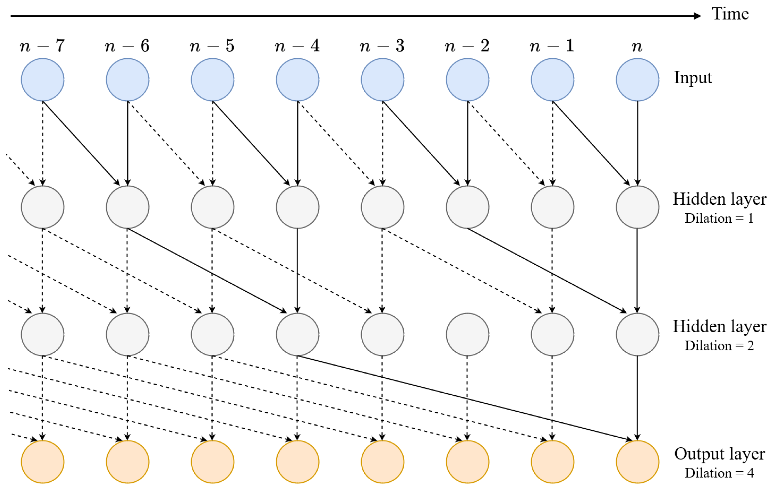
Table 1.
Feedforward WaveNet configuration summary. The nomenclature for these configurations is not generalized, and the names used here are taken from [26].
Table 1.
Feedforward WaveNet configuration summary. The nomenclature for these configurations is not generalized, and the names used here are taken from [26].
| Model | WaveNet 1 | WaveNet 2 | WaveNet 3 |
|---|---|---|---|
| Layers | 10 | 18 | 18 |
| Channels | 16 | 8 | 16 |
Table 2.
Summary of the architectures for distortion circuit modelling comprising recurrent, convolutional, and hybrid approaches.
Table 2.
Summary of the architectures for distortion circuit modelling comprising recurrent, convolutional, and hybrid approaches.
| Architectures | Details | Type |
|---|---|---|
| NARX | RNN modified for limited connectivity to avoid gradient problems. Used in [30] | Recurrent |
| Multi-layer LSTM | Used in [31] | Recurrent |
| 1 layer LSTM (150 units) + FC | Used in [35] | Recurrent |
| 2 layers LSTM (150 units) | Used in [35] | Recurrent |
| Sequence-to-sequence LSTM | Used in [35] | Recurrent |
| Parametric LSTM | Used in [35] | Recurrent |
| Convolutional LSTM | Used in [35] | Hybrid |
| 3-layer MLP | Used in [35] | DNN |
| CNN with pooling | Used in [35] | Convolutional |
| Convolutional RNN | Used in [35] | Hybrid |
| CAFx | DNN latent space [37] | Autoencoder |
| FeedForward WaveNet | Dilated convolutions used in [23,25,26] | Convolutional |
| CRAFx | Bi-LSTM latent space [39] | Autoencoder |
| Single-layer LSTM & GRU | Followed by FC layer [33] | Recurrent |
| CWAFx | WaveNet latent space [38] | Autoencoder |
| Shallow TCN | Used in [28] | Convolutional |
| STN | Gray-box MLP used in [41] | DNN |
| State-Space GRU | Gray-box RNN used in [42] | Recurrent |
Table 3.
Summary of the modelling approaches that utilize deep learning as well as their advantages and downsides.
Table 3.
Summary of the modelling approaches that utilize deep learning as well as their advantages and downsides.
| Approach | Pros | Cons |
|---|---|---|
| Black-Box |
|
|
| Gray-Box |
|
|
| White-Box |
|
|
Table 4.
Summary of the data sets used for training and their different characteristics.
| Data Set | Details |
|---|---|
| Custom | Function generator with frequencies ∈ [100 Hz; 500 Hz] + electric guitar fed to a vacuum tube amp; 96 kHz; stereo (1 channel input, 1 channel output) at 96 kHz used in [30] |
| Custom | Guitar into tube amplifier; 96 kHz; stereo used in [31] |
| Data set from [50] | Five different playing styles of guitar sounds passing through different amplifiers Used in [23,35,36] at 44.1 kHz |
| IDMT-SMT-Audio Effects [40] | 44.1 kHz used in [28] and downsampled to 16 kHz in [37,38,39] |
| Freesound [47] | Input signal sent through SPICE simulations at 44.1 kHz. Used in [25] |
| IDMT-SMT-Guitar/Bass [48,49] | Used in [23,26,33]. 44.1 kHz input signals sent through the analog target devices |
| SignalTrain [51] | Used in [28] at 44.1 kHz |
| Custom | Guitar signals sent through SPICE model of the analog circuit at 44.1 kHz used in [43] |
| Custom | 90-s logarithmic sine sweep ranging from 20 Hz to 20 kHz with constant amplitude followed by 90 s of white noise at 48 kHz used in [4] |
| Custom | 10-s logarithmic sine-sweeps combined with low-level white noise. This combined signal was increased in amplitude linearly from 0 to 1 over 1/2 the length of the signal. Min freq = 20 Hz and max = 10 kHz at 192 kHz [41] |
Table 5.
Summary of the loss functions and their perceptual relevance.
| Objective Function | Details |
|---|---|
| MSE | Non-perceptual, used in [31,41,43] |
| RMS | MSE based loss, non-perceptual, used in [30] |
| NRMSE | MSE based loss, non-perceptual |
| ESR + | Pre-emphasis for better high-frequency content in [25,26]. |
| ESR + | Studied for perceptual relevance in [53]. Includes DC offset. |
| ESR + | Studied for perceptual relevance in [53]. Includes DC offset. |
| ESR + | Studied for perceptual relevance in [53]. Includes DC offset and A-weighting. |
| MAE | Non-perceptual, used in [37,38,39] |
| STFT + MAE | Time-Frequency content, used in [28] |
Table 6.
Summary of the evaluation methods for network validation after training.
| Objective | Subjective |
|---|---|
| MSE [31], RMSE [30,35], NRMSE [35], Spectrogram [35,39], Power Spectrum [35], Harmonic Analysis using ESS [35], Waveform plot [23,33,35,39], SNR [35], Difference in harmonic content [35], MAE [37,38,39], FFT magnitude [39], Input-output waveshaping curves [39], ESR [23,25,26,33], MSED [37], Frequency spectrum [25,26], MS_MSE [38], MFCC_COSINE [38], Spectra of 1245-Hz sinusoid to study aliasing [26], AME [42], CT [23,25,26,35], Custom metric that takes into account RMSE + CT [35] | Aural comparison of prediction and target [31], 2 listening tests [35], MUSHRA [23,25], Web audio evaluation tool [38], pre-emphasized ESR [53] |
Table 7.
Summary of the real-time capabilities of each architecture in the state-of-the-art. We define the Real-Time factor here to be . RTF lower than 1 is required for real-time operation.
Table 7.
Summary of the real-time capabilities of each architecture in the state-of-the-art. We define the Real-Time factor here to be . RTF lower than 1 is required for real-time operation.
| Architecture | RTF | Sampling Rate (kHz) |
|---|---|---|
| NARX [30] | No mention | 96 |
| Multi-layer LSTM [31] | No mention | 96 |
| 1 layer LSTM (150 units) + FC [35] | 0.78 (GPU) | 44.1 |
| 2 layers LSTM (150 units) [35] | 1.39 (GPU) | 44.1 |
| Sequence-to-sequence LSTM [35] | 0.70 (GPU) | 44.1 |
| Parametric LSTM [35] | 0.71 (GPU) | 44.1 |
| Convolutional LSTM [35] | 0.45 (GPU) | 44.1 |
| 3-layer MLP [35] | 0.24 (GPU) | 44.1 |
| CNN with pooling [35] | 0.32 (GPU) | 44.1 |
| Convolutional RNN [35] | 0.45 (GPU) | 44.1 |
| CAFx [39] | No mention | 16 |
| FeedForward WaveNet amps [25] | 0.16 (WaveNet1) & 0.33 (WaveNet3) (Python) | 44.1 |
| FeedForward WaveNet pedals [26] | 0.53 (WaveNet1) & 0.91 (WaveNet3) (C++) | 44.1 |
| CRAFx [37,38] | 1.44 (Python-CPU) | 16 |
| Single-layer LSTM & GRU [33] | 0.097 for fastest RNN & 0.41 for slowest (estimated on CPU) | 44.1 |
| CWAFx [38] | 1.48 (Python-CPU) | 16 |
| Shallow TCN [28] | Capable of RT with a frame size of over 1024 for TCN-300-C & 4096 for TCN-324-N (Python-CPU) | |
| STN [41] | Estimated in terms of floating point operations and appears to be within the bounds of real-time | 192 |
| State-Space GRU [42] | No mention | 48 |
| Nercessian et al. [43] | No mention | 44.1 |
| Kuznetsov et al. [4] | Computed in terms of floating point operations | 48 |
| Esqueda et al. [46] | No mention but same RT capabilities as traditional White-Box | 96 |
Table 8.
Black-box architecture comparison. We define the Real-Time factor here to be . RTF lower than 1 is required for real-time operation. All results reported were recorded in Python on CPU (AMD Ryzen 7 3750H CPU at 2.3 GHz).
Table 8.
Black-box architecture comparison. We define the Real-Time factor here to be . RTF lower than 1 is required for real-time operation. All results reported were recorded in Python on CPU (AMD Ryzen 7 3750H CPU at 2.3 GHz).
| Architecture | RTF | MSE | ESR | MAE | STFT |
|---|---|---|---|---|---|
| RNN (LSTM-32) [33] | 0.51 | 0.0040 | 0.0244 | 0.0378 | 0.5952 |
| CNN (WaveNet) [25] | 0.35 | 0.0703 | 0.4337 | 0.1359 | 0.6542 |
| Hybrid (Conv-LSTM) [35] | 3.25 | 0.0069 | 0.0423 | 0.0530 | 0.6937 |
| CNN (Shallow TCN) [28] | 0.14 | 0.3190 | 2.1371 | 0.4510 | 1.2348 |
Publisher’s Note: MDPI stays neutral with regard to jurisdictional claims in published maps and institutional affiliations. |
© 2022 by the authors. Licensee MDPI, Basel, Switzerland. This article is an open access article distributed under the terms and conditions of the Creative Commons Attribution (CC BY) license (https://creativecommons.org/licenses/by/4.0/).
Share and Cite
MDPI and ACS Style
Vanhatalo, T.; Legrand, P.; Desainte-Catherine, M.; Hanna, P.; Brusco, A.; Pille, G.; Bayle, Y. A Review of Neural Network-Based Emulation of Guitar Amplifiers. Appl. Sci. 2022, 12, 5894. https://doi.org/10.3390/app12125894
AMA Style
Vanhatalo T, Legrand P, Desainte-Catherine M, Hanna P, Brusco A, Pille G, Bayle Y. A Review of Neural Network-Based Emulation of Guitar Amplifiers. Applied Sciences. 2022; 12(12):5894. https://doi.org/10.3390/app12125894
Chicago/Turabian StyleVanhatalo, Tara, Pierrick Legrand, Myriam Desainte-Catherine, Pierre Hanna, Antoine Brusco, Guillaume Pille, and Yann Bayle. 2022. "A Review of Neural Network-Based Emulation of Guitar Amplifiers" Applied Sciences 12, no. 12: 5894. https://doi.org/10.3390/app12125894
Note that from the first issue of 2016, this journal uses article numbers instead of page numbers. See further details here.