
Numerical Assessment of Side-Wind Effects on a Bus in Urban Conditions


Department of Building Services and Building Engineering, Faculty of Engineering, University of Debrecen, 4028 Debrecen, Hungary
Appl. Sci. 2022, 12(11), 5688; https://doi.org/10.3390/app12115688
Submission received: 9 May 2022
/
Revised: 28 May 2022
/
Accepted: 31 May 2022
/
Published: 3 June 2022
(This article belongs to the Special Issue Engineering Applications of Computational Fluid Mechanics (CFM))
Abstract
:The drag coefficient is usually considered to be a constant value, which allows us to calculate the aerodynamic losses. However, at lower speeds and wind, this value could be distorted. This also applies to buses in urban environments where due to traffic, the speed is relatively low. Since the schedule of the buses is fixed, based on the driving cycle, they travel at a nominal cruising speed. This makes it possible to examine the drag losses in a quasi-steady condition. To find the magnitude of this distortion in losses, a large-eddy simulation method was used with the help of commercially available software. Symmetrical and asymmetrical flows were induced into the digital wind tunnel to assess the distribution of the forces in the cruising direction and examine the flow patterns. It was discovered that the drag forces behave differently due to the low speeds, and calculations should be performed differently compared to high-speed drag evaluations.
1. Introduction
Fuel consumption of vehicles is dependent on many factors, so generally, it is highly unpredictable. This fact is attributed to the properties of the vehicle such as losses from the drivetrain, rolling, drag, and external factors such as the quality and slope of the road, traffic, and wind. By specifying the scenario and the vehicle, a more precise estimation can be made to give a consumer a more accurate view of the fuel consumption. By solely focusing on the relationship between the wind and aerodynamic losses of vehicles in general, a connection can be found, which could give a more precise prediction for fuel usage.
Drag loss calculation can be performed using multiple approaches. Barden et al. [1] made on-road measurements. They have attained a route-specific drag coefficient that corresponds to the average wind direction; thus, an average yaw angle for the location was concluded. It was shown that the wind tunnel underpredicts the drag losses by 33%, compared with an on-road scenario [1].
Side-wind studies are notably carried out on long ground vehicles such as trains, in which the high-speed stability is examined [2,3,4,5]. These high-speed trains due to safety concerns need to be examined when critical conditions occur; by contrast, at lower speeds, stability is not an issue. The abovementioned papers confirm that both the Reynolds averaged numerical simulation and large-eddy simulation give accurate predictions when forces are assessed. Howell et al. [6] showcased that the presence of side wind at a travelling speed of 27 m/s could increase the drag loss on vehicles.
In urban areas, the estimation of the actual flows is challenging, due to complex building shapes, trees, and rough terrain [7]. The numerical models in street canyons show that the wind speed is often negligible at near-ground level [8]. Due to the blockage effect of the buildings, a considerable amount of the mesoscale wind speed dropped to street level [9] even in extreme cases; nevertheless, some studies [10,11] indicated that when the blockage effect is negligible at street level, high velocities can be obtained. In a study by Tominaga et al. [12], it can be seen that at around two-metre height, the peaking velocity is around 1.4 m/s. For cars, it was indicated that even with a slight side wind, the flow structure and drag could change considerably [13].
Wind tunnel measurements are considered to be a baseline method and can be used for automotive measurements. However, necessary corrections have to be made such as the application of a belt system and rotating wheel [14,15]. Hobeika et al. [16] pointed out that detailing the tyre surface and adding rotation in numerical simulation could reduce drag by 4–5%, compared with wind tunnel measurement.
The movement of city buses is usually restricted by urban traffic and their schedule. During their operation, they often stop and cannot even reach the speed limit of the area. Using a driving cycle dataset, the average cruising speed can be found, which represents the closest steady state of that operation and can be applied for drag loss calculations. Vámosi et al. [17,18] mentioned that in the city of Debrecen, the average cruising speed is 19.197 km/h.
The scope of this assessment was to examine how much could a perpendicular wind load alter the drag losses of a city bus. The research was limited to constant travelling and wind speeds; thus, decelerations and accelerations, as well as wind gusts, were not examined. For low-Reynolds number flows, not many drag assessments have been carried out. This paper highlights what occurs with the aerodynamic loss when a bus is affected by a steady side wind.
Based on the literature review [17,18,19,20], common cruising and wind speeds in Debrecen were chosen as the input parameters. The model of the bus was created based on the schematics provided by the Public Transportation Company of Debrecen (DKV ltd.). Then, large-eddy simulations were made to examine the effect of the side wind on the bus.
2. Materials and Methods
This research focused on a bus located in Debrecen, Hungary. Thus, the typical bus geometry, the drive cycle, and the wind data were corresponding to this location for the sake of future on-road measurements.
2.1. Geometry
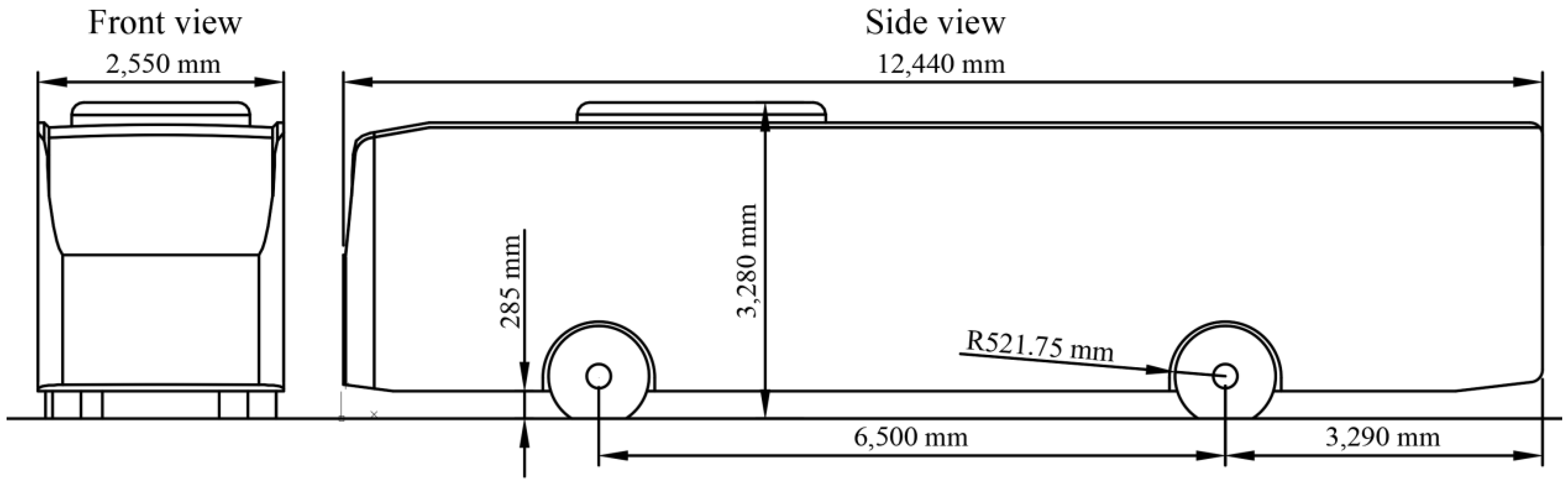
For vehicle geometry, a bus model was used which resembles the type Mercedes-Benz Reform 501 LE bus. The characteristic drawing was provided by DKV Ltd., and based on the sketch, further simplifications were made (see Figure 1). Mirrors, smaller holes, and finer details were not added. The base dimension in the domain was the total height of the vehicle H = 3280 mm. The tyres were type “295/80-R22.5”. Based on the sketch of the bus, it was assumed that a portion of the wheel was compressed by 81.75 mm.
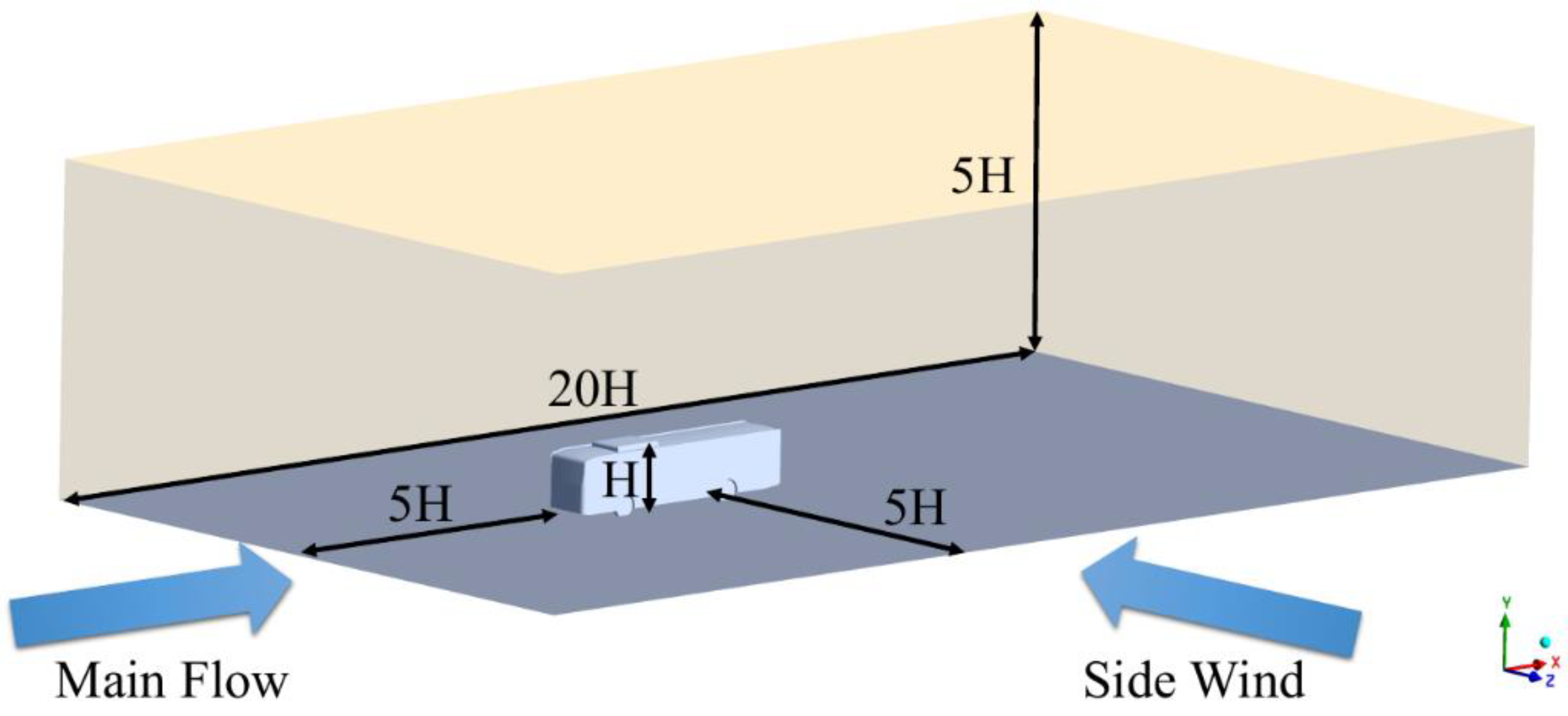
To describe the flow around the body an enclosure was made (see Figure 2), and the geometries were as follows: length 20 H, width 9 H, and height 5 H; at the front, 5 H long gaps were kept. It was assumed that behind the bus, a wake region could be generated; thus, during the discretisation, the rear surface of the bus was extended by 1 H length to serve as a refinement zone.
During the geometry design, the frontal area was determined using the geometry file, and the frontal projected area of the total bus was 7.80 m2.
2.2. Mesh
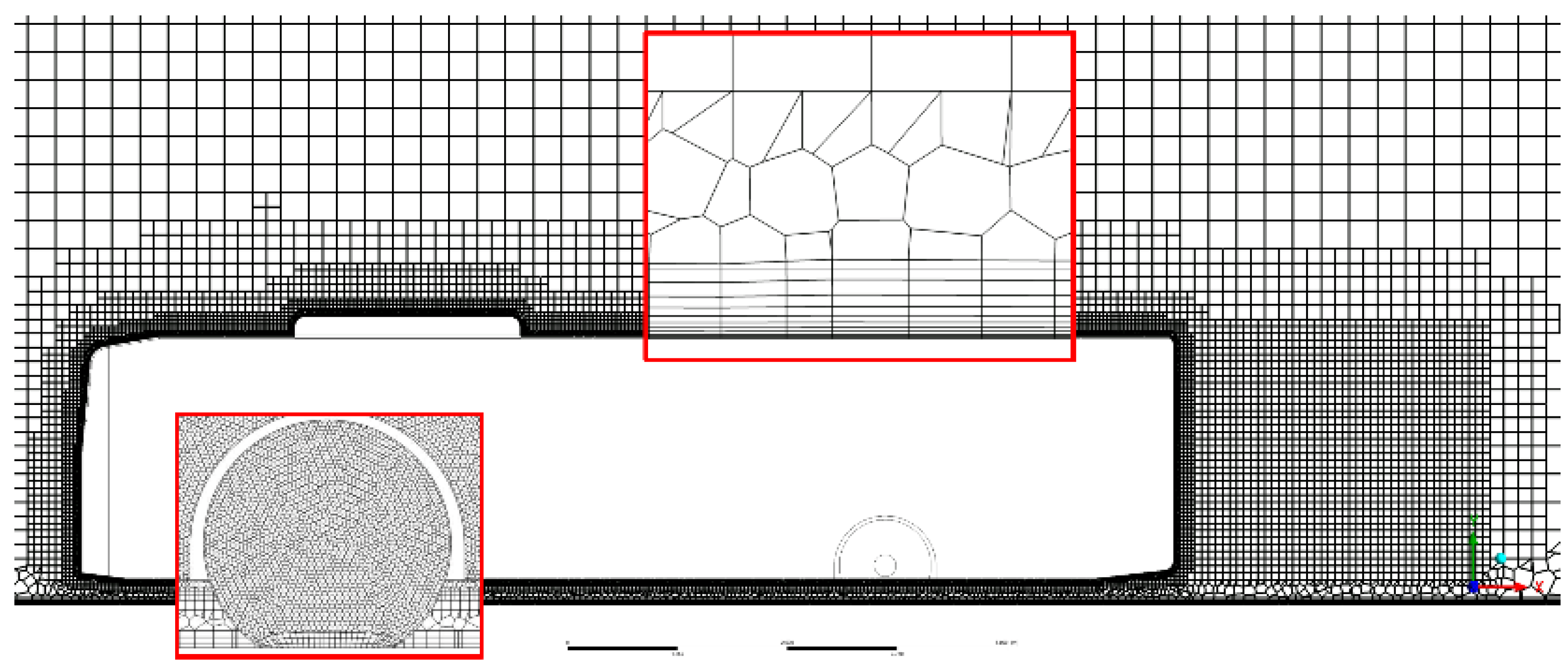
Further steps of the modelling were taken with ANSYS Fluent 2022 R1 (ANSYS Inc., Canonsburg, PA, USA) software. During the discretisation, three types of cells—hexagonal, polyhedral, and prismatic elements—were used. The core domain was built up from hexagonal mesh, while on the surface of the bus and on that of the ground prismatic layers were used. For transitioning between the surfaces and the hexagonal mesh, the polyhedral mesh was generated. To establish an adequate mesh, the following quality indicators were used: growth rate 1.2; maximum skewness 0.8, and minimum orthogonal quality 0.1. For mesh sensitivity analysis the first layer height (yH) and the maximum cell size (Δmax) were altered, as can be seen in Table 1. The almost linear increase in the cell count is attributed to the fact that by lowering the yH only the cell count of the refinement zone was increased, while the rest of the domain was less affected by the refinement.
In Figure 3, mesh2 can be seen. On the bus surface, ten pieces of prismatic layers were applied. For the ground, to ensure a smooth boundary layer three, levels of 20 mm high prismatic layers were applied. For the refinement zone behind the bus, a 100 mm large cell was used.
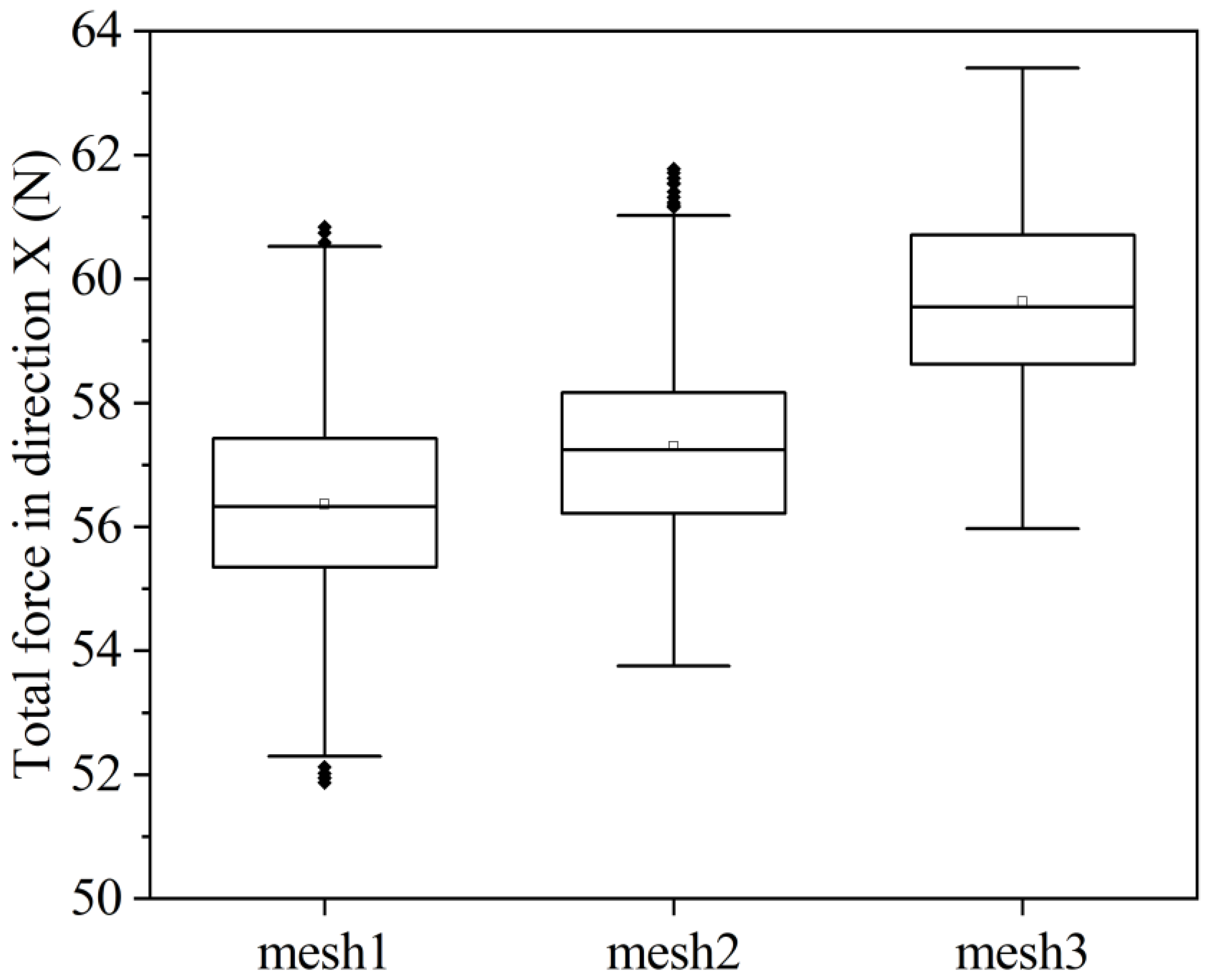
The sum of force components in the cruising direction exerted on the bus was used as a control value, and in this way, the mesh independency could be analysed. During the simulation, the forces showed unsteadiness; thus, the results are presented in a box plot (see Figure 4).
When the mean values of drag forces are compared, mesh2 showed a significant (4.08%) relative change compared with mesh3, while this tendency decreased (1.6%) with further refinement. One can see that the standard deviations of the drag forces decreased considerably (1.3% and 4.9%) with finer meshing. However, since the deviation was only 2.5% of the average value, it did not influence the final decision that mesh2 should be used in the further calculations.
2.3. Numerical Setup
The wall-adapting local eddy-viscosity–large-eddy simulation (WALE–LES) [21] method was chosen for the aerodynamic analysis. As to the low-velocity flow regime periodic alterations were expected, and an unsteady model was chosen. A further convergence analysis showed that the 0.05 s time step was enough to depict the unsteady deviations and converged results, yet coarse enough to considerably decrease the computational demand. The modelled duration was 80 s, during which at least 20 s was needed to initialise the flow, and 1 min of flow was examined; thus, the total number of time steps was 1600. The model was isothermal, and for velocity and pressure-based solver, the semi-implicit method for pressure-linked equations–consistent pressure–velocity coupling scheme was used. Furthermore, for pressure discretisation, PRESTO! was used, and for momentum and transient formulations, bounded central differencing was applied.
In Figure 2, two flows are indicated with blue arrows. The main flow represents the flow around the body of the bus; thus, it is assumed that the velocity is the cruising speed (vc) of the vehicle. If the wind comes in front of the bus, the velocity of the wind (vw) should be added to vc and subtracted, when it comes from behind the vehicle. The baseline cruising speed was attained from the bus driving cycle for Debrecen [17,18]. In the simulation, this value was rounded up to 20 km/h. While the mentioned value describes the nominal operation scenario, 10 km/h and 15 km/h cruising speeds were also assessed in the drag loss evaluation. Perpendicular to the main flow, side wind was also added to the model. This represents the most extreme condition, i.e., when the load on the vehicle is the most asymmetrical. Based on meteorological datasets [20], in the Debrecen city region, the most common wind speed (vw) is 2 m/s; to investigate the side-wind effects, 0 m/s, 1.5 m/s, and 1 m/s scenarios were also modelled. Furthermore, in Figure 2, the blue areas represent the velocity inlet boundaries, while the yellow ones the pressure outlet boundaries.
The ground and bus surfaces were no-slip walls, and to obtain a more realistic result, the ground and wheels were moving. The ground and shroud of the tyre had a wall velocity of the cruising speed. For the rim rotation, angular velocity was added, which was calculated from the cruising speed and the radius from the centre of the wheel. Since the surface velocities were corresponding to the cruising speed, it limited the research by assuming that the wind was always perpendicular to the bus.
In this study, two types of simulations were used; a symmetric one which is a classical wind tunnel simulation, where the main flow exerted force on the body, and an asymmetric one in which side wind was also added to the model. Symmetric scenarios were created to examine the differences between the 0 m/s inlet velocity and the symmetric boundary conditions. Thus, in the symmetric scenarios, the sides were set to symmetric (zero pressure inlet) conditions. In total, three symmetric and ten asymmetric simulations were carried out. The boundary condition settings are listed in Table 2.
3. Results
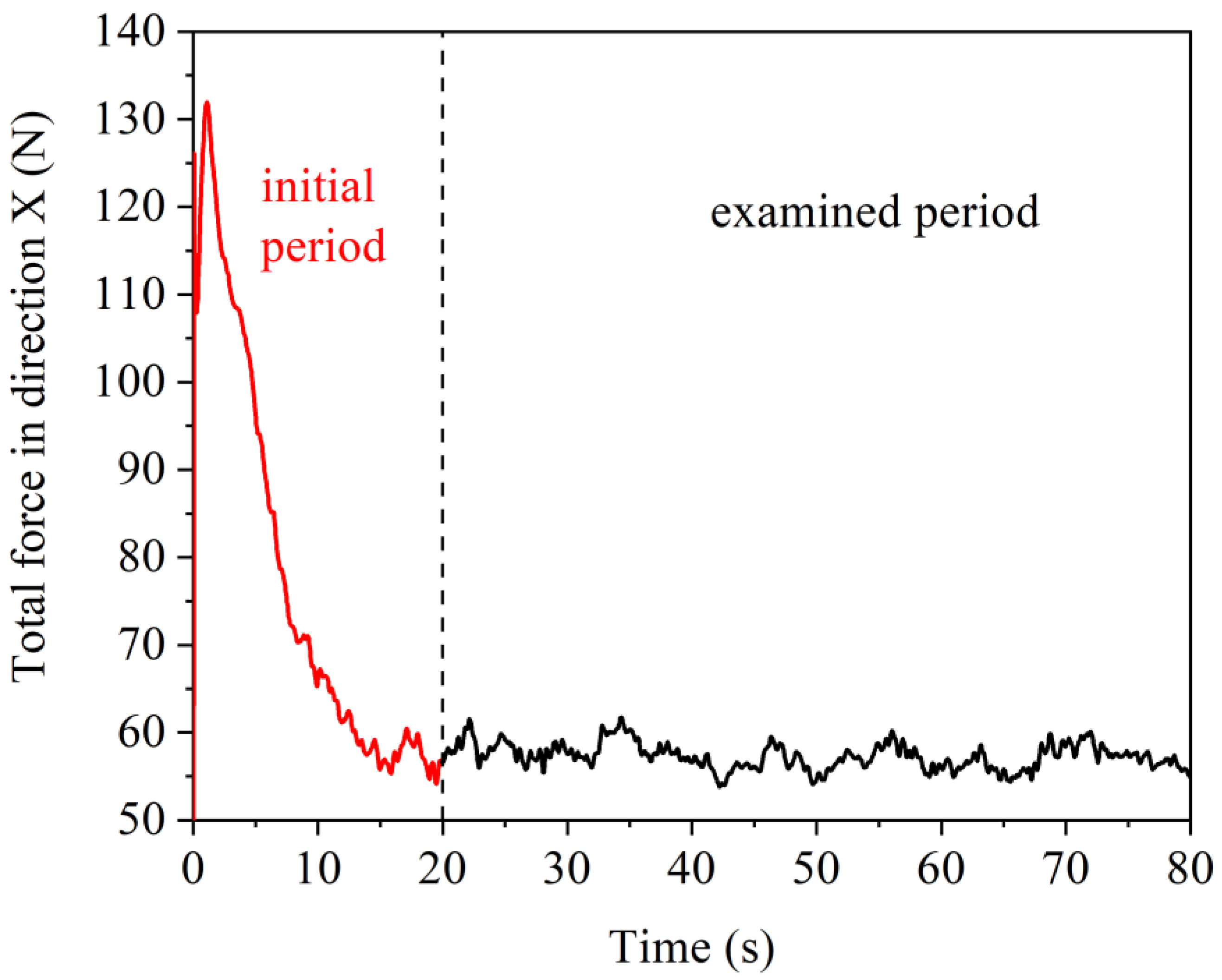
From the numerical models, the magnitudes of the force components of the cruising direction exerted on the bus (FX) corresponding to various velocities were assessed. It is worth noting that FX is not the classical drag force, since only the cruising direction component is used. The reason is that the X force component affects fuel consumption, while the others can affect the vehicle stability [22]. In Figure 5, one can see that, during the simulation, the sums of the forces fluctuated.
The fluctuation can be divided into two phases. First, when in the initial 20 s, a considerable number of changes occurred due to the development of the flow around the body of the bus. However, the residual values of the velocities were at a magnitude of 10−5 at the early stage of the solving process. Local convergence assessments showed highly deviating unsteadiness in most of the cases till the 20th second of flow time. Thus, in the assessment, the initial twenty-second period was disregarded, and only the last minute of the simulation was examined.
3.1. Obtained Force Values
In the simulations, FX forces were obtained from different surfaces of the bus and analysed. It can be noted that, in general, the median value of FX was also the most common; the peaking values only occurred on the frontal edge of the surface, where the corner vortices appeared. Along the length of the bus, this kind of FX deviation decreases.
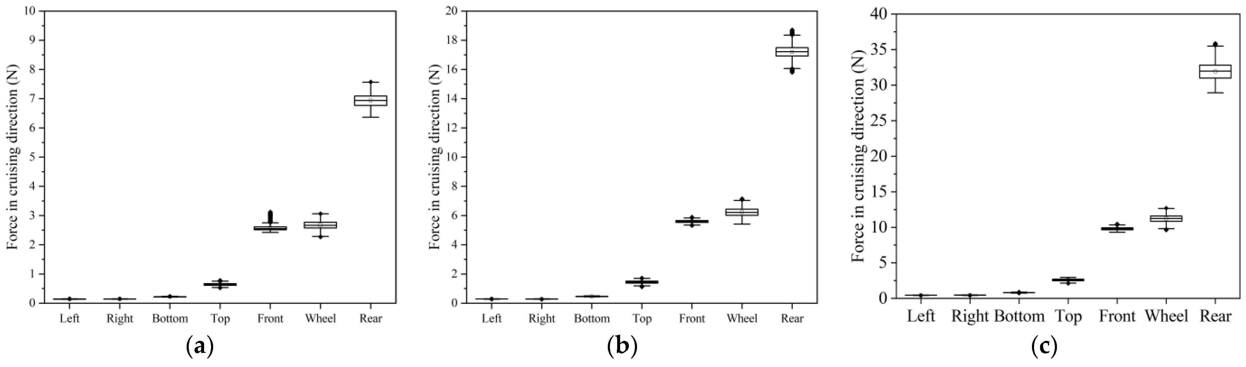
The presented results are the sums of the FX forces. When a high magnitude of the force was present, its effect could decrease due to the vortices. To analyse the force distribution on the bus (see Figure 6), the surface of the bus was divided into seven sections—left, right, frontal, bottom, top, wheels, and rear surfaces.
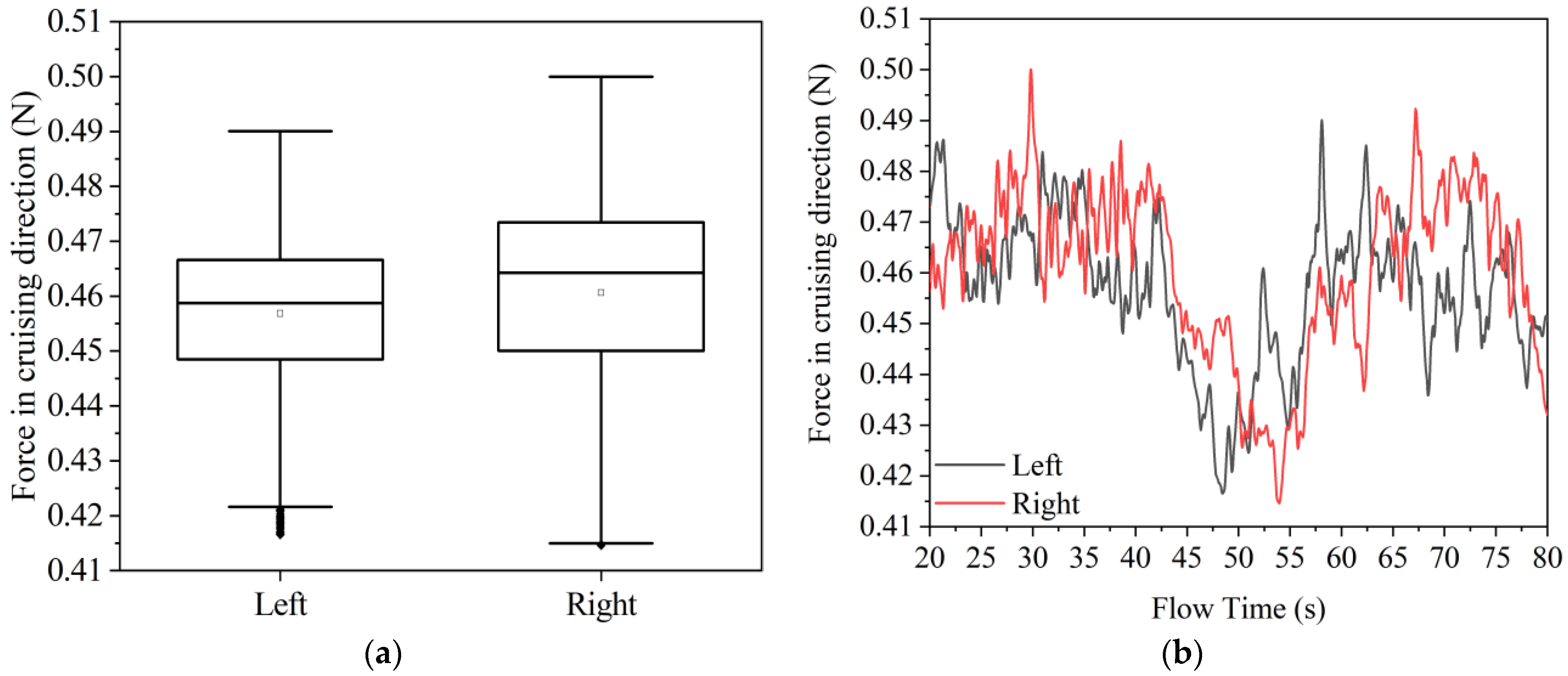
The FX force distribution shows that the rear surface and the wake region behind it generate most of the drag. It is also notable (Figure 6a) that, at 10 km/h on the frontal and wheel surfaces, the sums of the forces are relatively the same, while at higher speeds, the ratio of the front force decreases (Figure 6b,c). The lowest forces were obtained on the sides, which are magnified for the 20 km/h case in Figure 7.
The mean values are close to each other; however, the deviations are slightly higher on the right side. To examine it more closely, the FX and time connection is also plotted in Figure 7b. The two forces are altering symmetrically with a wavy trend. It could also be noted that on the right side, the increased deviation is due to the FX jump at the 30th second. The regression of the FX fluctuations, showed an R2 = 0.43 when it was examined for the sine function. Thus, further analyses were not made. Since consistent stochastic deviations were present, after the discussed values, the standard deviations were also added.
3.2. Asymmetric Flows
Before the analysis of the asymmetric flows, a comparison was made to determine the difference between symmetric and asymmetric simulation when on the sides—first symmetric and then inlet and outlet boundary conditions were used. The side wind blew on the left side of the bus. The sum of the Fx forces for both sides is presented in Table 3, together with their standard deviations.
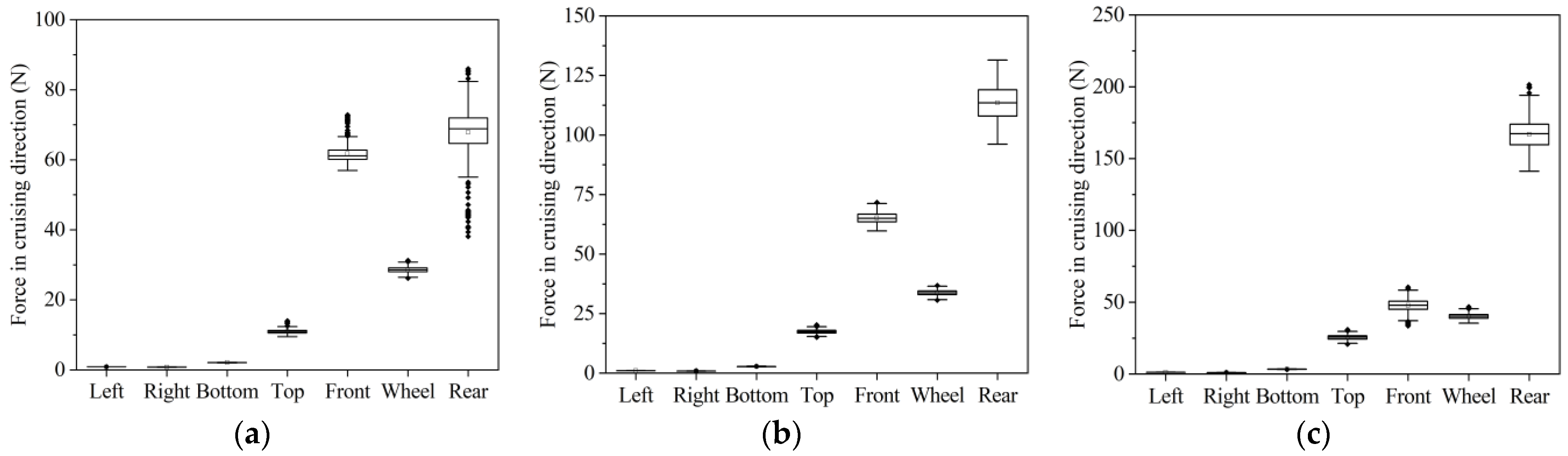
When no side wind was induced, only slight (0.82%) asymmetricity was noted, while in the most extreme case, a 32% change occurred on the sides. However, the forces changed on the sides as well as the other surfaces; thus, box plots were made to showcase them on the examined surfaces. It is noticeable from Figure 8 that the frontal force is considerably larger at lower wind speeds. The largest deviation occurred when the wind speed was 1 m/s, and compared with the forces on the other surfaces, it became roughly even at 2 m/s. By comparing the two extreme case with Figure 8b steady decrease can be seen. With the presence of this 2 m/s side wind, the FX increased five times on the bus.
3.3. Flow Formations
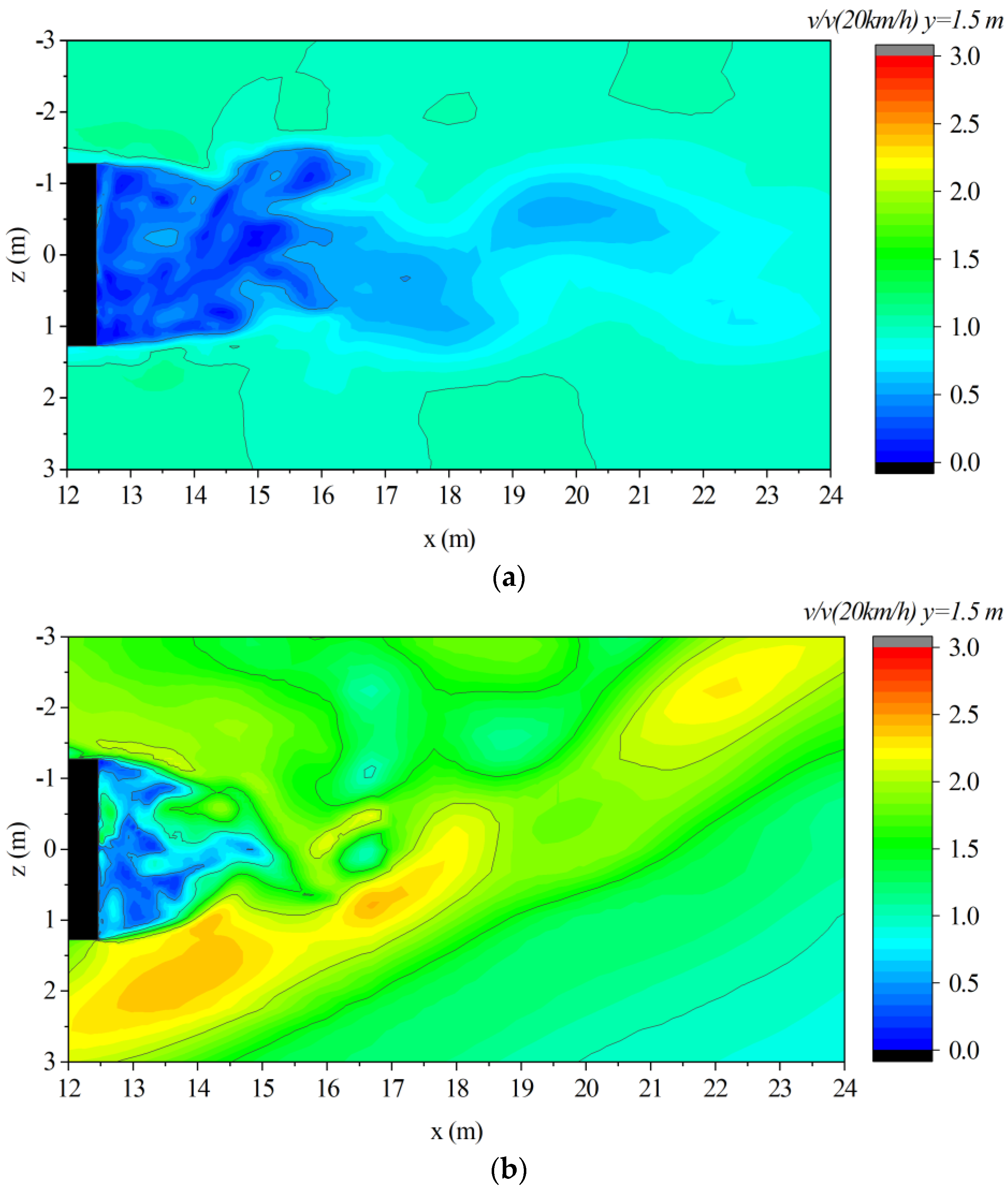
Since multiple magnitudes of flow velocities had been examined, only the 20 km/h velocity distribution was assessed horizontally and vertically. The horizontal velocity distribution at y = 1.5 m high was assessed in the two extreme side-wind cases: the symmetrical flow (Figure 9a) and the 2 m/s side-wind case (Figure 9b).
Even where the flow did not have any external influence, it showed an unsteady trait, as the vortex shedding can be seen in Figure 9a. When side wind was present, the average velocities were increased, most notably on the windward side (positive z region). When the bus was affected by the perpendicular wind load, the rear wake region was reduced. On the windward side of the bus, the vortex region was larger, which can be attributed to the fact that the surface of the bus altered the flow direction.
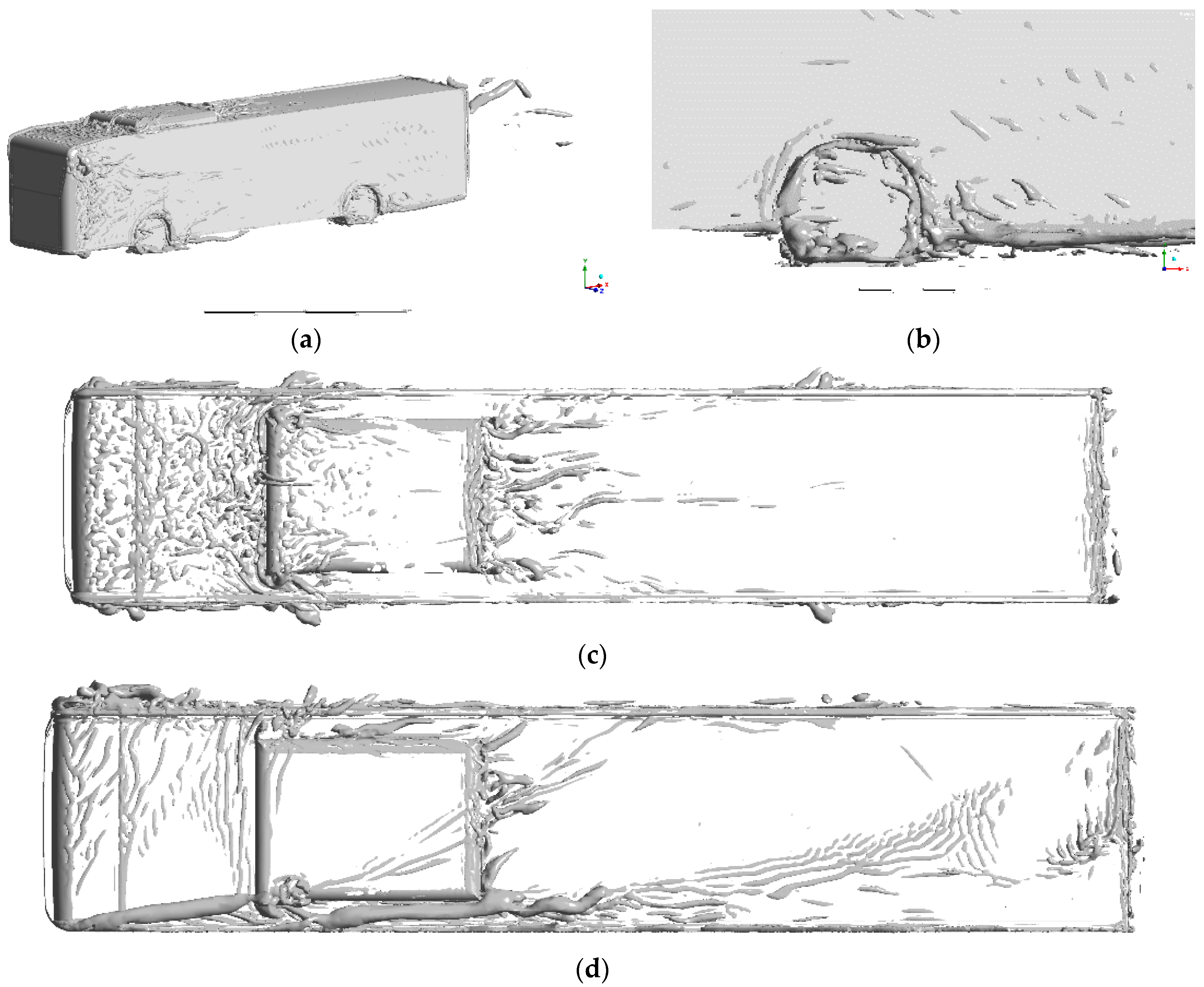
From the vertical plane (Figure 10a), it can be seen that the wake flow pattern is similar to what Lajos et al. [15] described. The stagnation point shifted to the lower section of the rear side of the bus. Over the range of x = 16–21 m, a small separated flow can be seen, which also strengthens the claim that the low-velocity flow makes force distribution uneven over time. It is also visible in Figure 10b that the wake region was reduced both horizontally and vertically. To assess the vortices, Q-criterion [23] was used to depict them, where Q is the second invariant of the velocity gradient tensor, and S and Ω are the symmetric and antisymmetric parts of the tensor and are expressed with Equation (2).
In Figure 11, large numbers of vortices were noted at the rear region and the wheel of the bus, at a Q-criterion value of 330 s−2.
It can be seen that due to the rounded corner at the front the corner, vortices were minimal. The bulk of the top air-condition unit generated most of the wakes beside the wheels and the rear region. The horseshoe vortices were not detected, which is a common flow structure at blunt bodies [24]. The Q-criterion values also indicate the asymmetrical pattern, mostly behind the air-conditioning box. On the windward side, large vortices were generated.
3.4. Validation
To compare the drag losses with other literature data, drag coefficient (CD) is used, which is calculated by the following equation:
where FX is the sum of the force components, A is the projection area, vc is the velocity of the bus in the cruising direction, and ρ is the density of air (1.225 kg/m3). The drag coefficient is only constant above a certain speed, around 100 km/h, and the CD of a bus is relatively high 0.66 [25]. Based on the geometry of the bus at lower speeds, the CD value could significantly decrease [26]. With the application of moving ground and wheels, Muthuvel et al. [27] attained CD = 0.43 with numerical and experimental methods. CD values, together with their standard deviations (due to its unsteady behaviour) from this study and other studies in the literature, are listed in Table 4.
The abovementioned combined results of numerical and experimental measurements are in good agreement with the current numerical results, considering that experimental results are rare in this velocity regime due to the decreased confidence of the force measuring appliances. Nevertheless, experimental measurements show that by decreasing the speed, the CD lowers [29].
With particle image velocimetry (PIV), Gurlek et al. [30] showed similar vertical flow patterns as that presented in Figure 10a, in which the lower recirculation bubble core is near the bottom edge of the bus, while the upper recirculation bubble has a longitudinal shape. However, the horizontal velocity distribution altered since, in this study, the rear wake region had unstable borders due to low speed.
In the work of Hobeika et al. [16], where rotating wheels were assessed, it was shown that in tyres with simplified wheel geometry, the Q-criterion had a similar pattern. With more details on the tyre, the vorticity region would become larger.
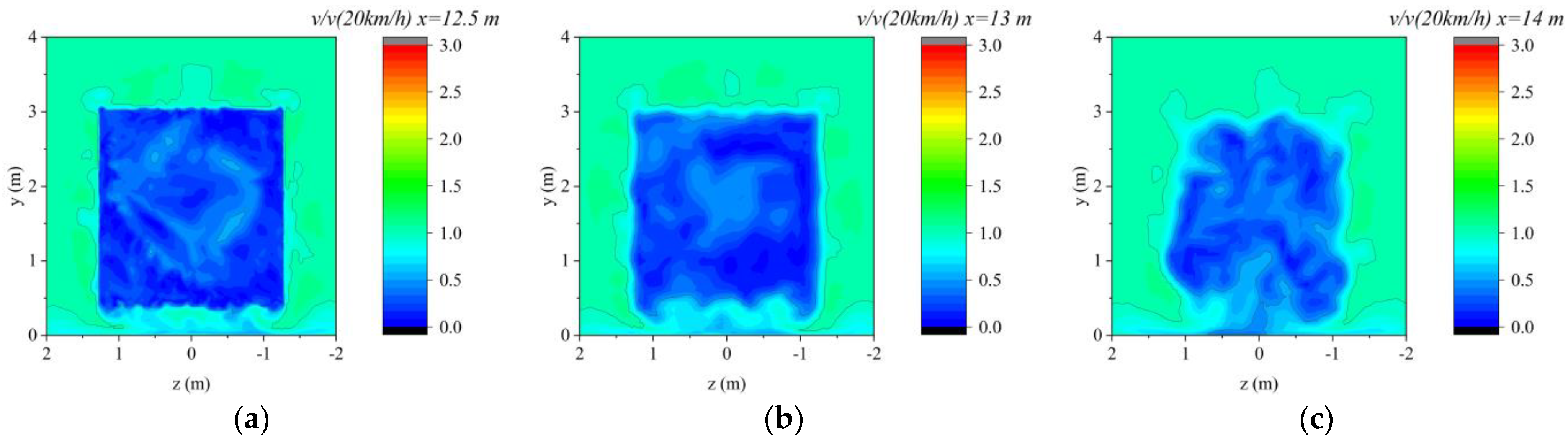
When velocity distribution of y–z vertical sections was assessed at x = 12.5 m, 13 m, and 14 m (see Figure 12), similar results were achieved as those reported in previous studies [15]. A comparison of the different sections indicates that, at the lower edge of the bus, longitudinal vortices were formatted. This similarity can be found in the work of Lajos et al. [15], though they showed higher velocities at the near ground level, while PIV measurement [30] indicates that similar longitudinal vortices occurred in this region (see Figure 12b). It is also notable that the mentioned lower vortices were moving upward, which corresponds to Figure 12c. These wake structures were also described in the work of Krajnovic et al. [31].
3.5. Drag Coefficients
While the 20 km/h cruising speed scenario is nominal, other cases were also modelled to study the drag changes. As was previously mentioned, the drag coefficient depends on velocity in the denominator, which is the cruising velocity of the vehicle, not the sum of the velocities corrected by the yaw angle. In Table 5, the drag coefficients with standard deviations are listed for different side-wind scenarios.
It can be seen that a notable jump occurred between symmetrical and 1 m/s side wind in all three speeds. At first, this is credited to the stagnation pressure increase at the low speeds; then, a relatively proportional increase followed at 20 km/h, while at lower cruising speeds, when side wind increased, CD slightly changed.
4. Discussion
The low-cruising speed creates a substantial deviation in drag, which also reduces the accuracy of the drag loss calculation. In the symmetric flow cases, the largest deviation was ±0.01, which corresponds to ±10 counts. Due to the already low CD value and the aerodynamically favourable geometry, further improvements to reduce the drag can be challenging with the existing methods [32]. It has to be noted that improvement below the deviation is considered to be an ineffective method.
Side winds and drag connections are an often researched field. Wieser et al. [13] and Howel et al. [6] showed that the drag increase at 41 m/s and 27 m/s resulted in around a 10–15% change in the drag coefficient. Compared with the results of this study, their drag coefficients are relatively lower than the showcased results. However, the assumption is that, at lower cruising speeds (5.55 m/s), the low wind speed (2 m/s) has a higher impact on the flow field and the drag than at higher cruising speeds.
The magnitude of the influence can be represented by velocity or drag coefficient triangles. When the bus travels at vc cruising speed and is affected by a perpendicular side wind (vw), the two vectors create a vT total velocity. This method can also be applied to the drag coefficient. Since drag coefficients were attained first for the symmetrical flows, a connection was established. Using exponential fitting on three highly deviating values (see Table 5) could give extremely large freedom; in spite of this, Equation (3) (R2 = 0.99) was defined.
where CDC is the drag coefficient at symmetrical flow. The next step was to evaluate the magnitude change due to the side wind. Frist to assess the difference between the CDT and CDC Equation (4) was used [33], to determine the magnitude of CDW the wind-induced drag.
Second, the CDW values were analysed and showed polynomial characteristics, with a regression of R2 = 0.91. The relation of the perpendicular side wind and side-wind-induced drag can be expressed with the following Equation (5):
When the results of Equation (4) were compared with those of the average drag equation used by Ingram [34], Equation (4) showed better agreement in the low-speed zone. The wind-averaged drag in the previously mentioned study was only valid above 9 m/s, and as a result, it underpredicts the CDT values, compared with the values of this study. It should be noted that the proposed Equations (3) and (5) are the most precise between 10 and 20 km/h.
By applying Equations (3)–(5) to the driving cycle, the actual aerodynamic losses can be calculated when the bus is cruising. In addition, by knowing the drag coefficient, the aerodynamic power demand can also be calculated by using Equation (6).
where the density of the air is 1.225 kg/m3. To generalise the result, the normalised power losses are shown in Table 6.
In the most extreme condition, the loss was 6.7 times larger than that in the symmetrical case. This effect exists in wind gusts, as well as in wind speeds that are present during 20–25% [19,20] time of the year. The normalised aerodynamic losses also indicate the extent of possible errors in measurements when speed (vc) is independently measured from the environment.
5. Conclusions
In this study, the aerodynamics of a bus was assessed in low-speed side-wind conditions with a large-eddy simulation method.
It was shown that the low cruising speed caused unsteady flow behind the bus and a ten-count deviation. This deviation made it difficult to use further drag reduction methods; only those could be applied which achieved higher improvement than ten counts. It can also be concluded that low cruising speed had an effect on reducing the drag coefficient. This phenomenon was strengthened by the results of other low-speed wind tunnel studies. When the asymmetrical flow was applied, major changes in drag force occurred on the frontal and rear surfaces of the bus, while at the windward and leeward, the changes were slight. Based on the numerical result, an equation was proposed for the total drag calculation.
The results also suggest that experts in the field should find a way to reduce the side wind that causes the drag on the vehicle and gather more wind data from the street level.
Funding
This research was financed by the Thematic Excellence Programme of the Ministry for Innovation and Technology in Hungary (ED_18-1-2019-0028), within the framework of the (Automotive Industry) thematic programme of the University of Debrecen.
Institutional Review Board Statement
Not applicable.
Informed Consent Statement
Not applicable.
Data Availability Statement
Not applicable.
Acknowledgments
The author expresses appreciation for DKV Ltd. for their kind help.
Conflicts of Interest
The author declares no conflict of interest.
References
- Barden, J.; Gerova, K. An on-road investigation into the conditions experienced by a heavy goods vehicle operating within the United Kingdom. Transp. Res. Part D Transp. Environ. 2016, 48, 284–297. [Google Scholar] [CrossRef]
- Diedrichs, B. Aerodynamic Calculations of Crosswind Stability of a High-Speed Train Using Control Volumes of Arbitrary Polyhedral Shape. In Proceedings of the BBAA VI International Colloquium on Bluff Bodies Aerodynamics & Applications, Milano, Italy, 20–24 July 2008; pp. 20–24. [Google Scholar]
- Rolén, C.; Rung, T.; Wu, D. Computational Modelling of Cross-Wind Stability of High Speed. In Proceedings of the European Congress on Computational Methods in Applied Sciences and Engineering, Jyväskylä, Finland, 24–28 July 2004. [Google Scholar]
- Fragner, M.M.; Weinman, K.A.; Deiterding, R.; Fey, U.; Wagner, C. Numerical and experimental studies of train geometries subject to cross winds. Civil. Comp. Proc. 2014, 104, 2015. [Google Scholar] [CrossRef] [Green Version]
- Wang, X.; Qian, Y.; Chen, Z.; Zhou, X.; Li, H.; Huang, H. Numerical studies on aerodynamics of high-speed railway train subjected to strong crosswind. Adv. Mech. Eng. 2019, 11, 1687814019887270. [Google Scholar] [CrossRef]
- Howell, J.; Forbes, D.; Passmore, M. A drag coefficient for application to the WLTP driving cycle. Proc. Inst. Mech. Eng. Part D J. Automob. Eng. 2017, 231, 1274–1286. [Google Scholar] [CrossRef] [Green Version]
- Torres, P.; Le Clainche, S.; Vinuesa, R. On the experimental, numerical and data-driven methods to study urban flows. Energies 2021, 14, 1310. [Google Scholar] [CrossRef]
- Lin, Y.; Hang, J.; Yang, H.; Chen, L.; Chen, G.; Ling, H.; Sandberg, M.; Claesson, L.; Lam, C.K. Investigation of the Reynolds number independence of cavity flow in 2D street canyons by wind tunnel experiments and numerical simulations. Build. Environ. 2021, 201, 107965. [Google Scholar] [CrossRef]
- Javanroodi, K.; Nik, V.M. Interactions between extreme climate and urban morphology: Investigating the evolution of extreme wind speeds from mesoscale to microscale. Urban Clim. 2020, 31, 2019. [Google Scholar] [CrossRef]
- Tomas, J.M.; Pourquie, M.J.B.M.; Jonker, H.J.J. Stable Stratification Effects on Flow and Pollutant Dispersion in Boundary Layers Entering a Generic Urban Environment. Bound. Layer Meteorol. 2016, 159, 221–239. [Google Scholar] [CrossRef] [Green Version]
- Dadioti, R.; Rees, S.J. Validation of open source cfd applied to building external flows. In Proceedings of the 14th International Conference IBPSA—Building Simulation 2015 (BS 2015), Hyderabad, India, 7–9 December 2015; pp. 826–833. [Google Scholar]
- Tominaga, Y.; Mochida, A.; Shirasawa, T.; Yoshie, R.; Kataoka, H.; Harimoto, K.; Nozu, T. Cross Comparisons of CFD Results of Wind Environment at Pedestrian Level around a High-Rise Building and within a Building Complex. J. Asian Archit. Build. Eng. 2004, 3, 63–70. [Google Scholar] [CrossRef]
- Wieser, D.; Nayeri, C.N.; Paschereit, C.O. Wake structures and surface patterns of the drivaer notchback car model under side wind conditions. Energies 2020, 13, 320. [Google Scholar] [CrossRef] [Green Version]
- Rejniak, A.A.; Gatto, A. Influence of Rotating Wheels and Moving Ground Use on the Unsteady Wake of a Small-Scale Road Vehicle. Flow Turbul. Combust. 2021, 106, 109–137. [Google Scholar] [CrossRef]
- Lajos, T.; Preszler, L.; Finta, L. Effect of moving ground simulation on the flow past bus models. J. Wind Eng. Ind. Aerodyn. 1986, 22, 271–277. [Google Scholar] [CrossRef]
- Hobeika, T.; Sebben, S. CFD investigation on wheel rotation modelling. J. Wind Eng. Ind. Aerodyn. 2018, 174, 241–251. [Google Scholar] [CrossRef] [Green Version]
- Vámosi, A.; Czégé, L.; Kocsis, I. Comparison of bus driving cycles elaborated for vehicle dynamic simulation. Int. Rev. Appl. Sci. Eng. 2021, 12, 86–91. [Google Scholar] [CrossRef]
- Vámosi, A.; Czégé, L.; Kocsis, I. Development of Bus Driving Cycle for Debrecen on the Basis of Real-traffic Data. Period. Polytech. Transp. Eng. 2022, 50, 184–190. [Google Scholar] [CrossRef]
- Angyal, A.; Ferenczi, Z.; Manousakas, M.; Furu, E.; Szoboszlai, Z.; Török, Z.; Papp, E.; Szikszai, Z.; Kertész, Z. Source identification of fine and coarse aerosol during smog episodes in Debrecen, Hungary. Air Qual. Atmos. Health 2021, 14, 1017–1032. [Google Scholar] [CrossRef]
- Huld, T.; Müller, R.; Gambardella, A. A new solar radiation database for estimating PV performance in Europe and Africa. Sol. Energy 2012, 86, 1803–1815. [Google Scholar] [CrossRef]
- Nicoud, F.; Ducros, F. Subgrid-scale stress modelling based on the square of the velocity. Flow Turbul. Combust. 1999, 62, 183–200. [Google Scholar] [CrossRef]
- Sekulic, D.; Vdovin, A.; Jacobson, B.; Sebben, S.; Johannesen, S.M. Effects of wind loads and floating bridge motion on intercity bus lateral stability. J. Wind Eng. Ind. Aerodyn. 2021, 212, 104589. [Google Scholar] [CrossRef]
- Hunt, J.C.R.; Wray, P.M.A.A. Eddies, Stream, and Convergence Zones in Turbulent Flows. In Proceedings of the Center for Turbulence Research, Summer Program; 1988; pp. 193–208. Available online: https://ntrs.nasa.gov/citations/19890015184 (accessed on 2 May 2022).
- Ahmed, S.R.; Ramm, G.; Faltin, G. Some Salient Features of the Time-Averaged Ground Vehicle Wake; SAE Transactions: Detroit, MI, USA, 1984. [Google Scholar] [CrossRef]
- Hamit, S.; Yakup, İ. Drag Coefficient Determination of a Bus Model Using Reynolds Number Independence. Int. J. Automot. Eng. Technol. 2015, 4, 146–151. [Google Scholar]
- Bayındırlı, C. Drag reduction of a bus model by passive flow canal. Int. J. Energy Appl. Technol. 2019, 6, 24–30. [Google Scholar] [CrossRef]
- Muthuvel, A.; Murthi, M.K.; Koshy, M.; Sakthi, S.; Selvakumar, E. Aerodynamic Exterior Body Design of Bus. Int. J. Sci. Eng. Res. 2013, 4, 2453–2457. Available online: http://www.ijser.org (accessed on 2 May 2022).
- Jadhav, C.R.; Chorage, R.P. Modification in commercial bus model to overcome aerodynamic drag effect by using CFD analysis. Results Eng. 2020, 6, 100091. [Google Scholar] [CrossRef]
- Janna, W.S.; Schmidt, D. Fluid Mechanics Laboratory Experiment: Measurement of Drag on Model Vehicles. In Proceedings of the 2014 American Society for Engineering Education Annual Conference & Exposition, Indianapolis, IN, USA, 15–18 June 2014. [Google Scholar]
- Gurlek, C.; Sahin, B.; Ozkan, G.M. PIV studies around a bus model. Exp. Therm. Fluid Sci. 2012, 38, 115–126. [Google Scholar] [CrossRef]
- Krajnović, S.; Davidson, L. Numerical study of the flow around a bus-shaped body. J. Fluids Eng. Trans. ASME 2003, 125, 500–509. [Google Scholar] [CrossRef]
- Szodrai, F. Quantitative Analysis of Drag Reduction Methods for Blunt Shaped Automobiles. Appl. Sci. 2020, 10, 4313. [Google Scholar] [CrossRef]
- Lorite-Díez, M.; Jiménez-González, J.I.; Pastur, L.; Cadot, O.; Martínez-Bazán, C. Drag reduction on a three-dimensional blunt body with different rear cavities under cross-wind conditions. J. Wind Eng. Ind. Aerodyn. 2020, 200, 104145. [Google Scholar] [CrossRef]
- Ingram, K.C. The Wind-Averaged Drag Coefficient Applied to Heavy Goods Vehicles; The National Academies of Sciences, Engineering, and Medicine: Washington, DC, USA, 1978; Available online: https://trid.trb.org/view/80996 (accessed on 2 May 2022).
Figure 1.
Schematic of the bus.

Figure 2.
Sideview of the bus.

Figure 3.
Vertical cross-section view of mesh2.

Figure 4.
Results of mesh sensitivity analysis.

Figure 5.
Total drag force fluctuation over time.

Figure 6.
FX forces on the bus at (a) 10 km/h; (b) 15 km/h; (c) 20 km/h.

Figure 7.
(a) FX forces on the side of the bus at 20 km/h box plot; (b) force–time connection.

Figure 8.
Asymmetric FX forces on the side of the bus at 20 km/h for (a) 1 m/s, (b) 1.5 m/s, (c) and 2 m/s side winds.
Figure 8.
Asymmetric FX forces on the side of the bus at 20 km/h for (a) 1 m/s, (b) 1.5 m/s, (c) and 2 m/s side winds.

Figure 9.
Horizontal velocity distributions at 1.5 m height for 20 km/h (a) symmetrical flow and (b) 2 m/s side wind.
Figure 9.
Horizontal velocity distributions at 1.5 m height for 20 km/h (a) symmetrical flow and (b) 2 m/s side wind.

Figure 10.
Vertical velocity distributions at 20 km/h on the symmetry plane for (a) symmetrical flow and (b) 2 m/s side wind.
Figure 10.
Vertical velocity distributions at 20 km/h on the symmetry plane for (a) symmetrical flow and (b) 2 m/s side wind.

Figure 11.
Q-criterion distribution on (a) the bus and (b) near wheel; (c) symmetrical flow; (d) asymmetrical flow.
Figure 11.
Q-criterion distribution on (a) the bus and (b) near wheel; (c) symmetrical flow; (d) asymmetrical flow.

Figure 12.
Velocity distribution at (a) x = 12.5 m, (b) 13 m, and (c) 14 m y–z vertical sections.


Table 1.
Mesh properties.
| Cases | yH | Δmax | Cell Count |
|---|---|---|---|
| Mesh1 | 0.25 mm | 160 mm | 13.6 × 10⁶ |
| Mesh2 | 0.5 mm | 320 mm | 6.5 × 10⁶ |
| Mesh3 | 1 mm | 640 mm | 4.4 × 10⁶ |
Table 2.
Boundary conditions.
| Type | Magnitude | Comment |
|---|---|---|
| Frontal inlet | Cruising speed | Constant velocity inlet |
| Ground | Cruising speed | No-slip moving wall |
| Tyre surface | Cruising speed | No-slip moving wall |
| Rim | Cruising speed/radius | No-slip rotating wall |
| Side inlet | Wind speed | Constant velocity inlet |
| Outlet | 1 atm total pressure | Pressure outlet |
| Bus | - | No-slip stationary wall |
| Top | - | Symmetry condition |
Table 3.
FX on the left and right sides with different side-wind boundary conditions.
| Side-Wind Condition | FXLeft (N) | FXRight (N) | FXLeft-FXRight (N) |
|---|---|---|---|
| Symmetric | 0.457 ± 0.014 | 0.461 ± 0.017 | −0.004 |
| 0 m/s | 0.388 ± 0.016 | 0.44 ± 0.017 | −0.052 |
| 1 m/s | 0.863 ± 0.006 | 0.796 ± 0.035 | 0.067 |
| 1.5 m/s | 1.076 ± 0.006 | 0.922 ± 0.041 | 0.154 |
| 2 m/s | 1.302 ± 0.007 | 0.983 ± 0.059 | 0.319 |
Table 4.
Drag coefficients.
| Drag Coefficient | Comment | Source |
|---|---|---|
| 0.362 ± 0.009 | 10 km/h | Current study |
| 0.380 ± 0.008 | 15 km/h | Current study |
| 0.389 ± 0.010 | 20 km/h | Current study |
| 0.65 | 36 km/h | Cihan Bayındırlı [26] |
| 0.43 | 80 km/h | Muthuvel et al. [27] |
| 0.66 | 100 km/h | Hamit et al. [25] |
| 0.65 | 120 km/h | Jadhav et al. [28] |
| 0.41 | modified | Jadhav et al. [28] |
Table 5.
Drag coefficients at different side-wind and cruising speed magnitudes.
| Side-Wind Speed | 10 km/h | 15 km/h | 20 km/h |
|---|---|---|---|
| symmetric | 0362 ± 0.009 | 0.380 ± 0.008 | 0.389 ± 0.010 |
| 1 m/s | 1.986 ± 0.065 | 1.418 ± 0.044 | 1.173 ± 0.044 |
| 1.5 m/s | 2.425 ± 0.174 | 2.110 ± 0.061 | 1.591 ± 0.053 |
| 2 m/s | 2.305 ± 0.236 | 2.318 ± 0.105 | 1.927 ± 0.082 |
Table 6.
Normalised aerodynamic losses at different side-wind speeds at different cruising speeds.
| Side-Wind Speed | Ṗ/Ṗ10 km/h | Ṗ/Ṗ15 km/h | Ṗ/Ṗ20 km/h |
|---|---|---|---|
| 1 m/s | 5.49 | 3.73 | 3.02 |
| 1.5 m/s | 6.699 | 5.55 | 4.09 |
| 2 m/s | 6.37 | 6.10 | 4.95 |
Publisher’s Note: MDPI stays neutral with regard to jurisdictional claims in published maps and institutional affiliations. |
© 2022 by the author. Licensee MDPI, Basel, Switzerland. This article is an open access article distributed under the terms and conditions of the Creative Commons Attribution (CC BY) license (https://creativecommons.org/licenses/by/4.0/).
Share and Cite
MDPI and ACS Style
Szodrai, F. Numerical Assessment of Side-Wind Effects on a Bus in Urban Conditions. Appl. Sci. 2022, 12, 5688. https://doi.org/10.3390/app12115688
AMA Style
Szodrai F. Numerical Assessment of Side-Wind Effects on a Bus in Urban Conditions. Applied Sciences. 2022; 12(11):5688. https://doi.org/10.3390/app12115688
Chicago/Turabian StyleSzodrai, Ferenc. 2022. "Numerical Assessment of Side-Wind Effects on a Bus in Urban Conditions" Applied Sciences 12, no. 11: 5688. https://doi.org/10.3390/app12115688
Note that from the first issue of 2016, this journal uses article numbers instead of page numbers. See further details here.