
Unique Features of Nonlocally Nonlinear Systems with Oscillatory Responses


1
Guangdong Provincial Key Laboratory of Nanophotonic Functional Materials and Devices, South China Normal University, Guangzhou 510631, China
2
School of Physics and Electrical Information, Shangqiu Normal University, Shangqiu 476000, China
3
College of Science, South China Agriculture University, Guangzhou 510642, China
*
Author to whom correspondence should be addressed.
Appl. Sci. 2022, 12(5), 2386; https://doi.org/10.3390/app12052386
Submission received: 26 August 2021
/
Revised: 8 February 2022
/
Accepted: 8 February 2022
/
Published: 25 February 2022
(This article belongs to the Special Issue Light Beams in Liquid Crystals)
Abstract
:We review the recent investigation of a new form of nonlocally nonlinear system with oscillatory responses. The system has various new features, such as the nonlocality-controllable transition of self-focusing and self-defocusing nonlinearities, a unique modulational instability and new forms of solitons. We also discuss the propagation of the optical beam in a nematic liquid crystal with negative dielectric anisotropy and demonstrate theoretically that propagation can be modelled by the system.
PACS:
42.65.Jx; 42.65.Tg; 42.70.Df; 42.65.Ky1. Introduction
The optical Kerr effect (OKE), a phenomenon that refers to the dependence of the refractive index on the optical intensity, is one of the most important effects in nonlinear optics [1,2]. The physical mechanism of OKE includes molecular reorientation, thermal nonlinearity, photorefractive effect, electronic contribution and electrostriction, etc. No matter what the physical mechanism is, the caused refractive index can always be phenomenologically represented as , with and being, respectively, the linear refractive index and nonlinear refractive index (NRI). If NRI at a certain point in space is not determined solely by the optical intensity at that point but also depends on its vicinity, nonlinearity is spatially nonlocal [3,4,5]. Mathematically, NRI can be expressed as an integral of a kernel function (also called the response function) and an optical intensity [3]. The media of nonlocal nonlinearity are referred to as nonlocally nonlinear media [6,7,8,9], which ranges from nematic liquid crystal (NLC) with positive dielectric anisotropy [10,11,12,13,14], lead glass [15], nonlinear ion gas [16], photorefractive crystal [17], dipolar Bose–Einstein condensate [18] and so on. For the physical systems mentioned above, response functions are positive definite, for example, the exponential-decay response function for the (1 + 1)-dimensional case [19] and the zeroth-order modified Bessel function for the (1 + 2)-dimensional infinite case [10,20].
In fact, there is the other kind of response function without positive definiteness: the sine-oscillation function, brought out in the study of quadratic solitons by the formal equivalence in mathematics between quadratic and nonlocal solitons [21,22]. This kind of sine-oscillation function was also obtained in a system of coupled Gross–Pitaevskii–Poission equations [23], which govern the evolutions for matter–wave components and the microwave magnetic field in atomic Bose–Einstein condensates. Recently, we investigated the nonlocally nonlinear system with oscillatory responses [24,25,26,27,28,29,30,31,32] and found various new features such as the nonlocality-controllable transitions between focusing and defocusing nonlinearities, unique modulational instabilities (MI) and new kinds of solitons. The nonlocally nonlinear system with oscillatory responses can model the propagation of optical beams in NLC with negative dielectric anisotropy.
In this review article, we provide a brief overview of unique features of nonlocally nonlinear system with oscillatory responses, including its mathematical model, the treatment of the model and the nonlocality-controllable transition between focusing and defocusing nonlinearities in Section 2, the short-term and long-term MI properties in Section 3, different kind of soliton solutions in Section 4 and a special algorithm for finding soliton solutions in Section 5. In Section 6, we discuss the nonlinearity characteristic of NLC with negative dielectric anisotropy and show that it can be modeled by the nonlinear system with oscillatory responses.
2. Nonlocality-Controllable Kerr Nonlinearities
The model we considered is the dimensionless system in the form of [27,28]
The equations are the coupled equations for a dimensionless optical beam and its (dimensionless) induced NRI , where is D-dimensional transverse coordinate vectors ( or 2), is the D-dimensional transverse Laplacian operator, is the sign of Kerr coefficient and is the nonlinear characteristic length. We will show in Section 6 that the model, Equation (1) plus (2), can describe the evolutions of optical beams in the NLC with negative dielectric anisotropy. However, the model discussed extensively before is the following [3,5]:
of which the second term has different signs from that of Equation (2). It is such a difference in the signs that makes the two nonlinear systems described by Equations (2) and (3) exhibit utterly different features.
Although the NRI described by Equation (2) in an infinite space can also be expressed by the following convolution:
similarly to the case of Equation (3) [3,5], the D-dimensional response function is completely different. When , the response takes the sin-oscillatory function as [27]
While, when [28], the response function is expressed by the following:
with being the zeroth order Bessel function of the second kind. Substituting Equation (4) into Equation (1) yields a nonlocally nonlinear Schrödinger equation in the form of
We can glimpse at the self-focusing and self-defocusing property of the nonlinear system described by Equation (7) from two limits where and . When , Equation (2) is reduced to . Clearly, the focusing nonlinearity occurs for and the defocusing nonlinearity does for . When , Equation (2) changes to , which models the focusing nonlinearity in lead glass for [15] and the defocusing nonlinearity for . Therefore, the nonlinearities reverse if proceeds from 0 to ∞ for both cases of . This indicates that the self-focusing and self-defocusing property of the nonlinear system described by Equation (7) depends on the degree of nonlocality, which is defined by with w being the beam width [27]. In contrast, for the nonlinear system given by Equation (3), the self-focusing and self-defocusing property is different. In the case where , Equation (3) is reduced to when , and to when . Under the two limits, the system (3) exhibits both self-focusing nonlinearity: that is, the local self-focusing nonlinearity when and the (thermally induced) nonlocal self-focusing nonlinearity in lead glass [15]. Conversely, in the case where , the self-defocusing nonlinearity exists for the two limits of . Therefore, no nonlinearities transition can take place in the nonlinear system given by Equation (3).
The dependence of the self-focusing and self-defocusing property on the degree of nonlocality can be obtained by both the variational approach and by numerical simulations. The Lagrangian density of the system described by Equation (7) is the following: [33,34]
We introduce a trial Gaussian beam:
where all meanings of parameters and c can be found in Ref. [28]. According to the standard procedure of variational approach [33,34], we obtain the evolution of the beam width w [28]:
where is the input power, and the mathematical expression of can be found in Ref. [28]. By assuming and , Equation (10) can be solved:
where . For linear propagations of the input Gaussian beam, the beam width is widened to be [35]. If the beam is in a focusing state, its width is , while in a defocusing state it is . Therefore, when nonlinearities transit between focusing and defocusing as the degree of nonlocality changes, by replacing w with in Equation (11) transition point can be obtained as
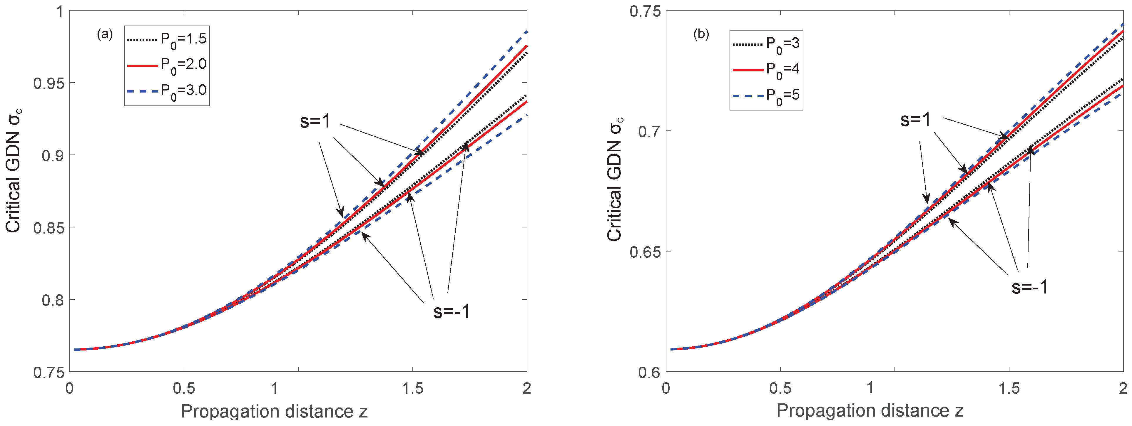
Equation (12) provides an implicit function of the critical degree of nonlocality on z, , s and D. For a given and , the function can be obtained by numerically solving the integral Equation (12) at different propagation distances z, which is shown in Figure 1.
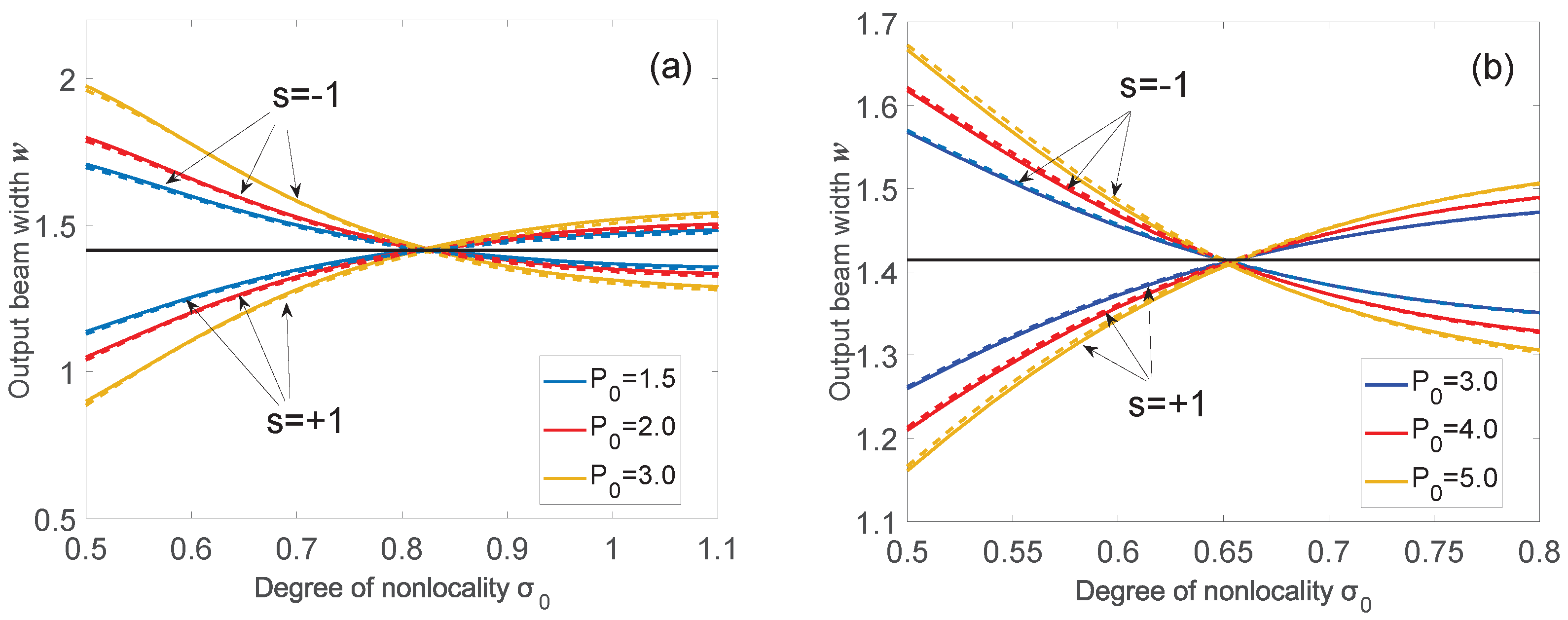
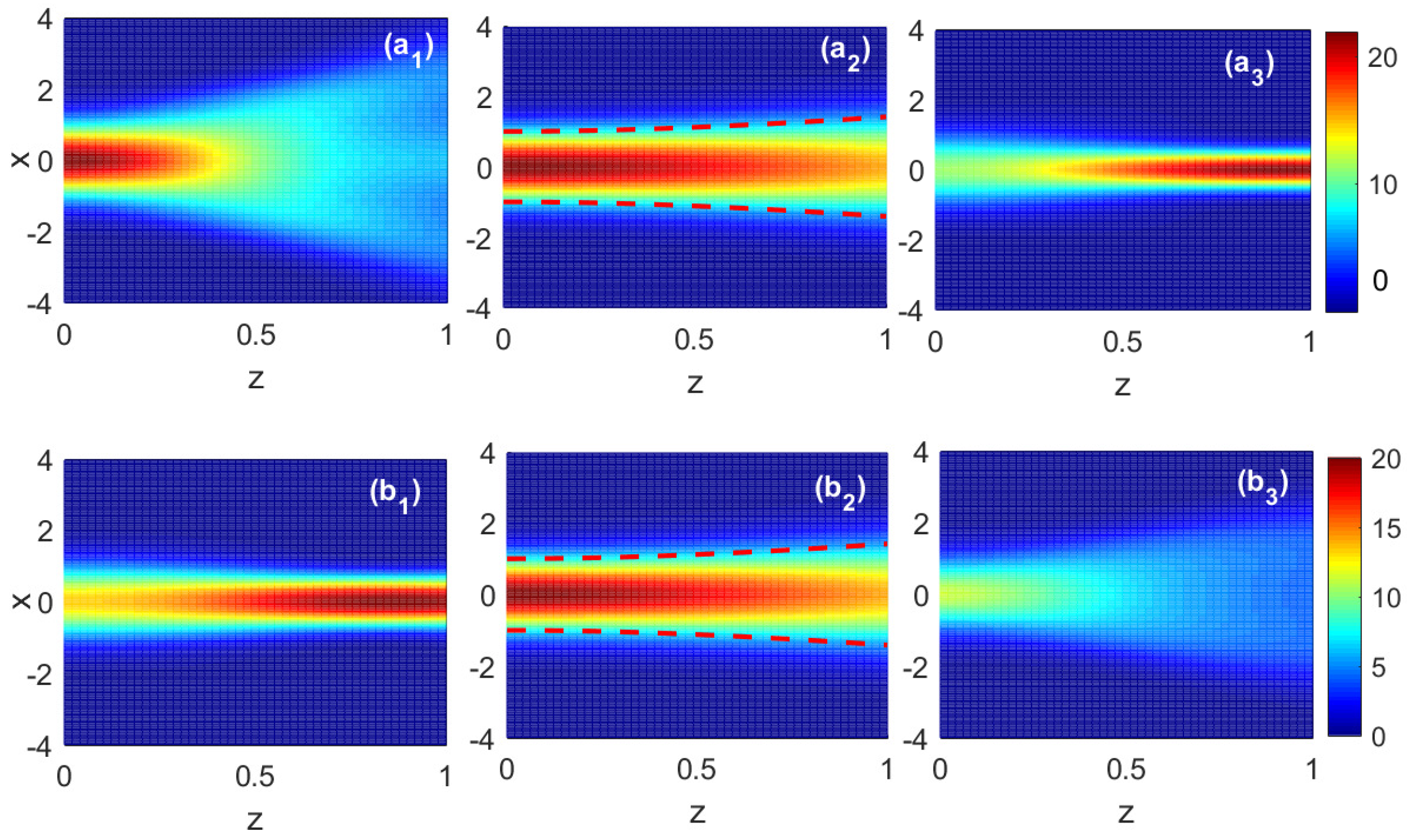
At the specific distance , the critical degree of nonlocality for the - and -dimensional cases can be obtained from Equation (12) in that and , respectively. The dependence of beam width on the degree of nonlocality is given in Figure 2. For the case of , optical beams experience self-defocusing nonlinearity when , and self-focusing nonlinearity when . The case of is on the contrary. Figure 3 shows the evolutions of the optical beam for different degree of nonlocality in two cases of and , where the degree-of-nonlocality-dependence self-focusing and self-defocusing effects can be obviously observed.
3. Unique Modulational Instability
In this section, we briefly review the modulational instabilities (MI) of the (1 + 1)-dimensional nonlocally nonlinear system (7) with oscillatory response (5). The evolution of perturbations we investigated includes two processes: short-term evolution and long-term evolution. During the short-term evolution of MI, the perturbation is small enough so that the linear analysis on the NNLSE (7) is valid [31]. However, after the optical field evolves for long term, the increasing perturbation is not much lower than the amplitude of plane wave, and the linear approximation method is not applicable, and the nonlinear evolution of MI should be considered: that is, the long-term evolution of MI [32].
3.1. Short-Term Evolution of MI
According to the standard procedure [36], we add a random perturbation () on the plane wave:
where and represents the Fourier transform of the response function (5). After calculations, the gain coefficient of perturbation is obtained as follows [31]:
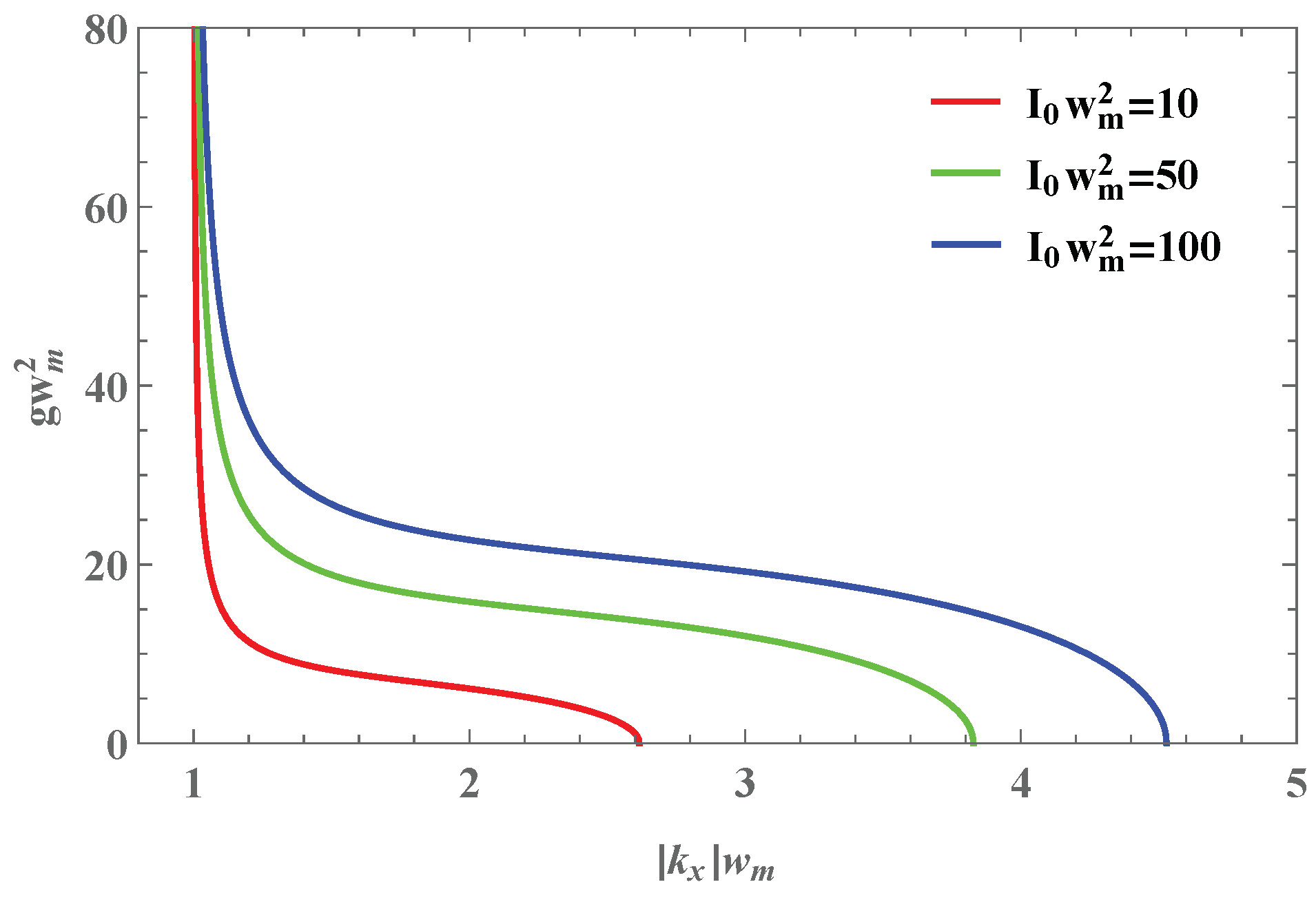
which only exists when . When , MI occurs when the following is the case:
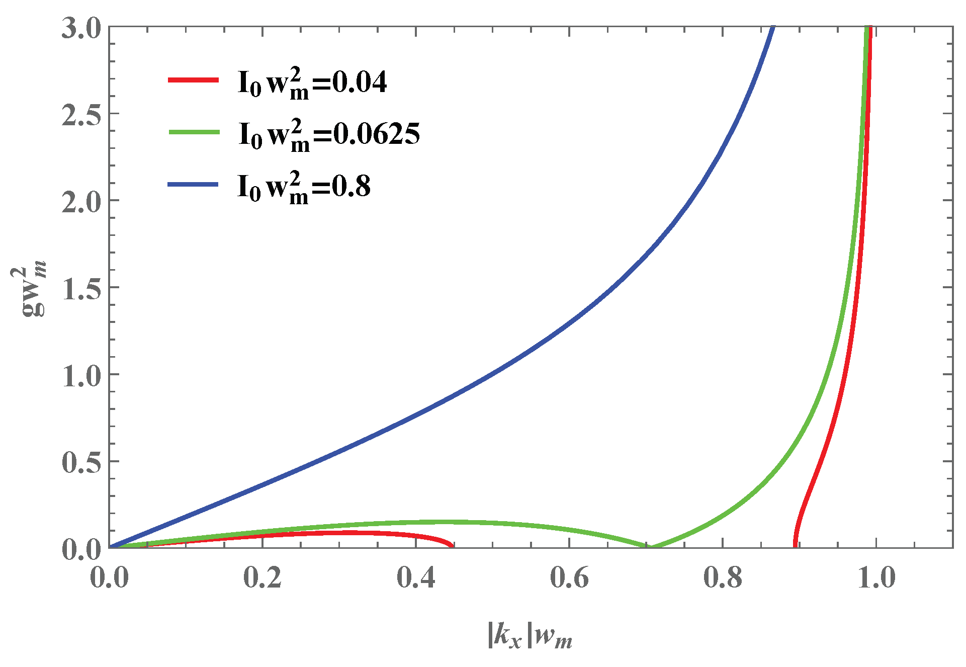
which is shown Figure 4. When and the light intensity is small enough to meet the following condition:
there are two MI gain bands, as shown in Figure 5, at each side of the origin.
Furthermore, after exceeds the critical value of , the MI gain bands combine into one as follows:
which is shown Figure 5. MI in the nonlocally nonlinear system with oscillatory responses is found to have two unique properties. First, MI exists both when the Kerr coefficient is positive and when it is negative. Second, the maximum gain points of MI do not shift with light intensity. The physical mechanism behind the properties of MI has been revealed by utilizing the theory of four-wave mixing in Ref. [31].
3.2. Long-Term Evolution of MI
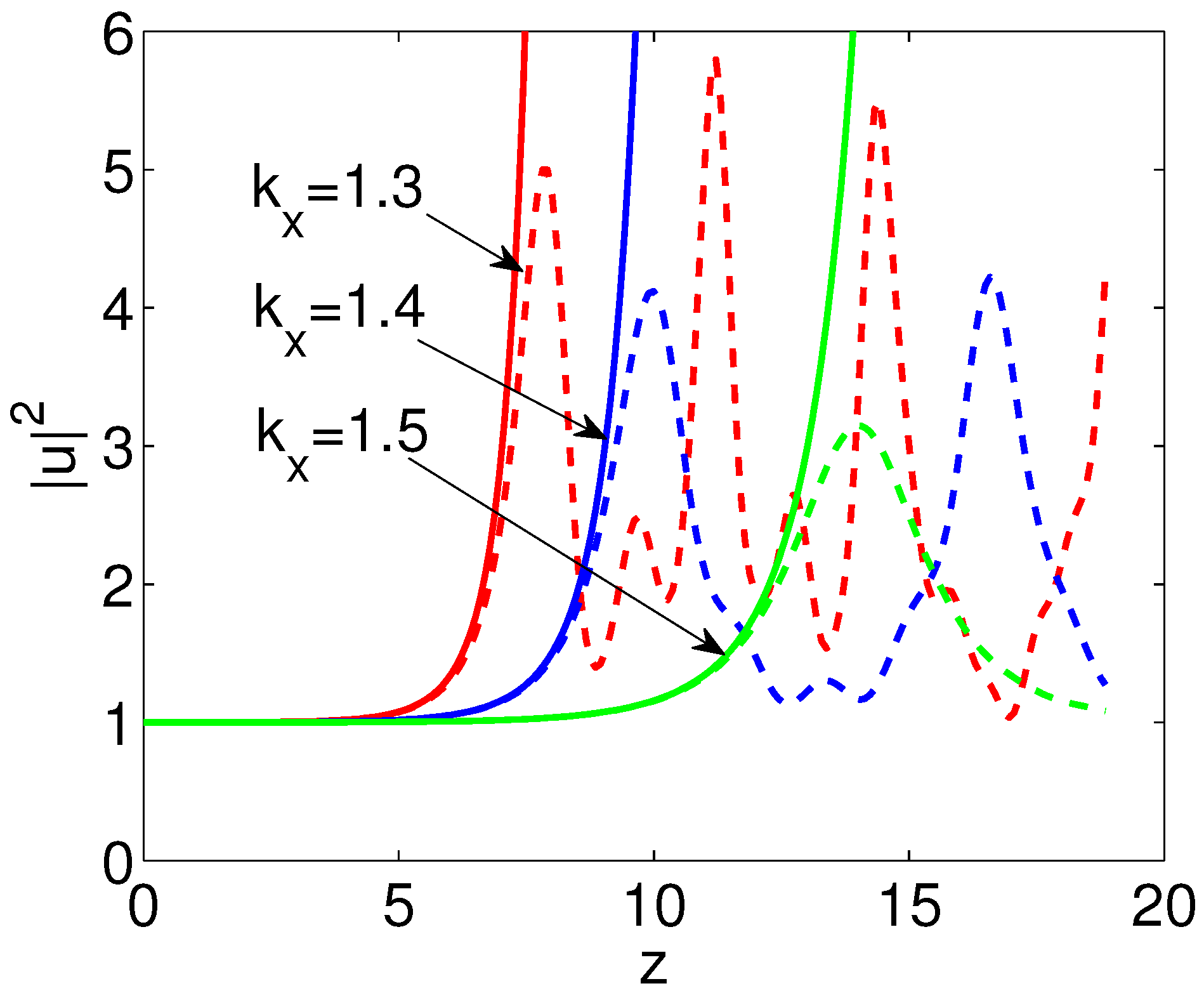
To show the long-term evolution of MI, we take an infinite plane wave with perturbation [32]:
as the initial input of Equation (7) with and , where the first term, the second term and represent plane wave, perturbation and frequency of perturbation, respectively. In the following numerical simulation, we assume that and . Then, MI appears in the range of . is the singular point at which the gain coefficient g is infinite and is the cutoff point. The nonlinear evolutionary process of initial input (19) of different perturbation frequencies is shown in Figure 6. In the short-term evolution, the curve of intensity obtained through linear processing is consistent with the numerical simulation, which means that linear approximation is applicable. However, in long-term evolution, the results obtained by linear approximation gradually deviated from numerical simulations. Additionally, the perturbation of the frequency close to the singular point increases more quickly to a larger peak; by contrast, the perturbation of the frequency close to the cutoff point presents a slower growth of a lower peak. The reason why the numerical simulations deviate from the analytical result is that, during the nonlinear evolutions of perturbation higher-order, harmonic waves appear. In this case, the linear approximation of perturbation is not appropriate, and harmonic waves with higher frequencies should be taken into account.
We can obtain the stable solution of induced MI by considering the input modulated wave to be composed of harmonics with various frequencies:
For stable solutions, the amplitudes of various harmonic do not vary with propagation distance z; then, we assume . Substitution into Equation (7) with and yields the following:
If only the first harmonic is taken into account, the analytical solution to Equation (20) can be obtained as
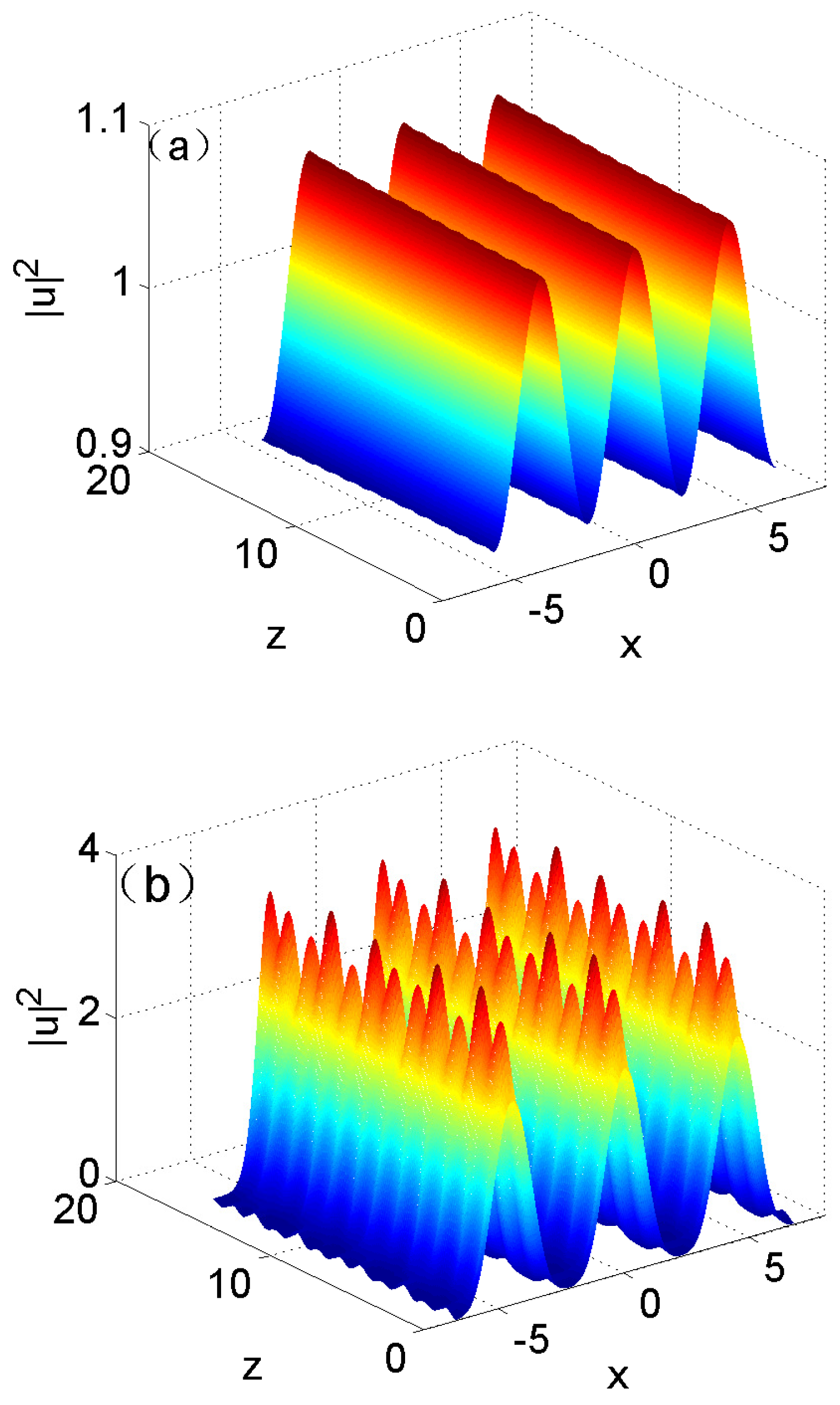
By using as the initial conditions, the evolution of stable solution is displayed in Figure 7. As shown in the figure, only the solutions when the modulation frequency is near the cutoff frequency are able to be stably propagated, while the ones when the modulation frequency departs from the cutoff frequency will fluctuate greatly during propagations; in this case, an increased number of harmonics should be considered. In this case, it is impossible to obtain the analytical solution, and the numerical method is required in order to solve Equation (20) [32].
4. Characteristics of Solitons
The MI of the nonlocally nonlinear system (7) always exists for cases of [31]. In consequence, due to the MI [36], the dark solitons [27,37] in self-defocusing sides of such a nonlocally nonlinear system are unstable [27], while the bright solitons existing in self-focusing sides can propagate stably. Concretely, in the case of , self-focusing and self-defocusing nonlinearities are, respectively, exhibited in high and low ranges of the degree of nonlocality, while in the case of , the self-focusing and self-defocusing properties are on the contrary. In the following, we will review our works on the bright solitons in the self-focusing sides of such a system described by Equation (7) in cases of . In addition to fundamental solitons [27,28], there are new kinds of solitons including the in-phase and out-of-phase bound-state solitons [29] and multi-peak (more than four peaks) solitons [30] in the nonlocally nonlinear system with oscillatory responses.
The variational approach is used to obtain the approximate solutions of bright solitons, including the fundamental solitons [28] and and Hermite–Gaussian-type multi-peak solitons [30]. The variational results have been confirmed by the numerical ones. We used the imaginary time evolution method to iterate the fundamental solitons [27,28] and the in-phase and out-of-phase bound-state solitons [29]. To iterate the multi-peak solitons with arbitrary peak numbers [30], we specifically developed a perturbation-iteration method [38].
4.1. Fundamental Solitons
The soliton solutions correspond to the extremum points of the equivalent potential [28,33]; therefore, by allowing the critical power of the solitons can be obtained as
It should be noted that, in Equation (23), the critical power must be positive, which requires for and for . Furthermore, the solitons are stable at the minimum points of , then we have:
From Equation (24), the existence ranges of the degree of nonlocality for the solitons can be determined, which depend on the values of D and the sign of s. When , the solitons exist if for and for . When , the existence ranges of are for and for . These variational results agree well with the numerical ones, which are given in the following.
In order to numerically iterate the soliton solution, we assume . Substitution of the solution into Equations (1) and (2) yields the following:
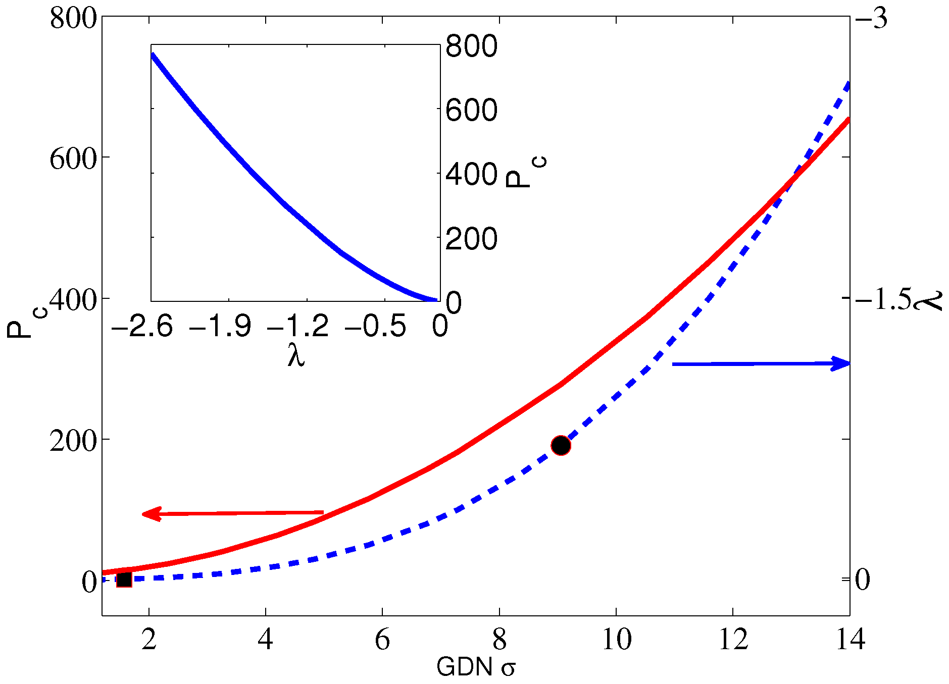
By the imaginary-time method, the solitons can be numerically found in higher ranges of the degree of nonlocality, for and for in the case of . These ranges of are all within the self-focusing sides of such a nonlinear system and agree well with the variational results. The bright solitons have two abnormal properties. The first one is the negative propagation constants, while it is the opposite of the cases in local nonlinear media [39] and nonlocally nonlinear media with the positively defining attenuating response functions [3]. The other is the negative slope of the ( and being the critical power and the propagation constant), as shown in Figure 8. By means of linear stability analysis, all solitons are shown to be stable [27]. This means that the stability criterion obeys an anti-Vakhitov–Kolokolov stability criterion [40], which is also obeyed by the in-phase and out-of-phase bound-state solitons and the multi-peak solitons reviewed in the next two sections. However, in nonlocally nonlinear media with the positively defining attenuating response functions, stable solitons should comply with the Vakhitov–Kolokolov criterion [9]. We have noticed that the evolutions for matter–wave components and the microwave magnetic field in the atomic Bose–Einstein condensates can also be governed by the mathematical model of Equation (1) plus (2) with in some specific conditions [23,41,42], and in such a system, bright solitons are obtained in strongly nonlocal cases.
Although what Equations (25) and (26) determine are the solitons of the nonlocally nonlinear system (7), the coupled equations with are formally the same as the model governing parametric spatial solitary waves in quadratic nonlinear materials [21,22,43]. The fundamental and the second harmonic waves are mathematically equivalent to the paraxial beam and its induced NRI [21]. Esbensen et al. employed the formal equivalence between two distinct physical systems to investigate the stabilities of solitons and found that the solitons are all unstable. However, it should be noted that equivalence is limited only to the solitary waves, while their dynamic properties, such as the stability, are completely different. In quadratic nonlinear materials, there is the energy and phase exchange between the fundamental and the second harmonic waves. Therefore, for the second harmonic wave, its z-dependant evolution should be taken into account, which is not the case for the NRI shown in Equation (2). Detailed discussions on this point can be found in Ref. [10]. Our group also made some improvements on the issue of quadratic solitons [24,25,26]. We found that the boundary confinement of media can support stable solitons [24]. Furthermore, the fundamental waves even can be multipole solitons [25], the existence of which depends closely on the sample size and the degree of nonlocality. If nonlocality is fixed and the sample size is varied, soliton width varies piecewise and approximately periodically [26].
4.2. In-Phase and Out-of-Phase Bound-State Solitons
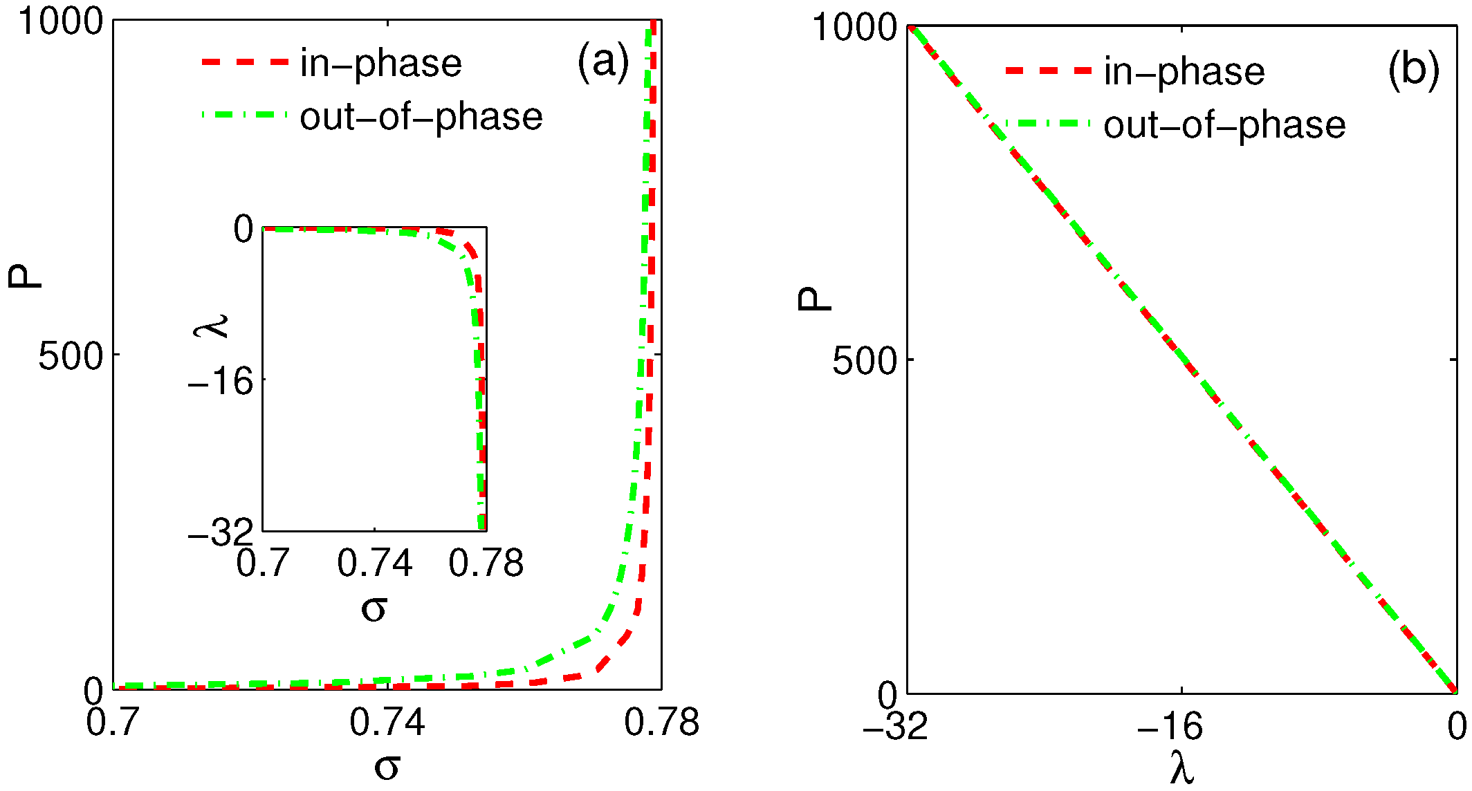
In the case of , the nonlinear system exhibits self-focusing nonlinearity in lower ranges of degree of nonlocality, that is, . In these ranges, we obtained bright solitons with complicated structures, which are the in-phase bound-state solitons when and the out-of-phase bound-state solitons when [29]. The in-phase bound-state soliton, shown in Figure 9, owns the symmetrical profile and the nonzero central value. On the other hand, the out-of-phase bound-state soliton, shown in Figure 10, owns the antisymmetrical profile and the zero central value. When the degree of nonlocality decreases, the in-phase bound-state soliton approaches the sech profile shown in Figure 9, and the out-of-phase bound-state soliton tends toward the first-order Hermite–Gaussian profile shown in Figure 10. The above-mentioned abnormal properties in the previous section, that is, the negative propagation constants and the negative slope of the power-propagation constant (the so-called anti-Vakhitov–Kolokolov stability criterion), also exist for bound-state solitons, which is shown in Figure 11a. Furthermore, it can be found from Figure 11b that the power-propagation constant diagrams are the same for both the in-phase and the out-of-phase bound-state solitons. In other words, we can say that two forms of bound-state solitons form degenerate modes.
4.3. Multi-Peak Solitons
The Hermite–Gaussian soliton solutions with multipeaks in fact have been discussed in nonlocally nonlinear media with positively-definiting attenuating response functions [44,45]. However, the upper thresholds of the peak number of the stable solitons in nonlocally nonlinear media are different, which closely depend on the response function of media. For instance, in the nonlocal system with the Gaussian response, the multipeak solitons with any peak number [4] are stable [44]. In nematic liquid crystals with positive dielectric anisotropy, the response function is an exponential decay one for the case, and the peak-number of the solitons supported is only less than five [44]. In the nonlocally nonlinear system with oscillatory responses described by Equations (1) and (2), we found the upper thresholds of the peak number of the stable solitons are five and four in the cases of and 1, respectively [30].
The variational approach can be applied to find solitons and discuss their stabilities. The Hermite–Gaussian solitons of the -dimensional NNLSE (7) are of the following profiles:
The critical power is obtained as follows:
where function is the given in Ref. [30]. The degree of nonlocality range within which HG solitons exist is obtained by the variational approach, which is summarized in Table 1, where the numerical results are also given for a comparison.
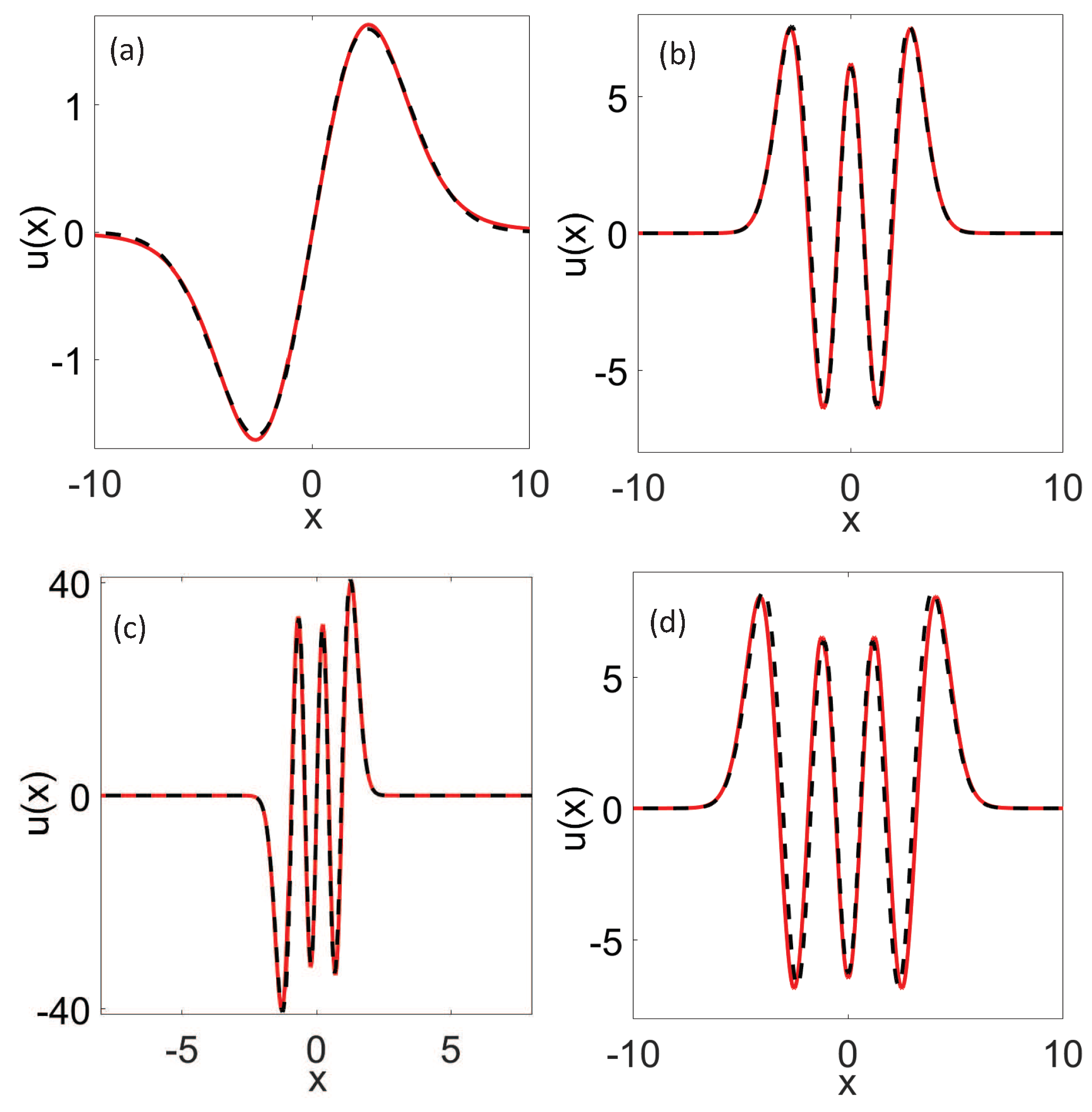
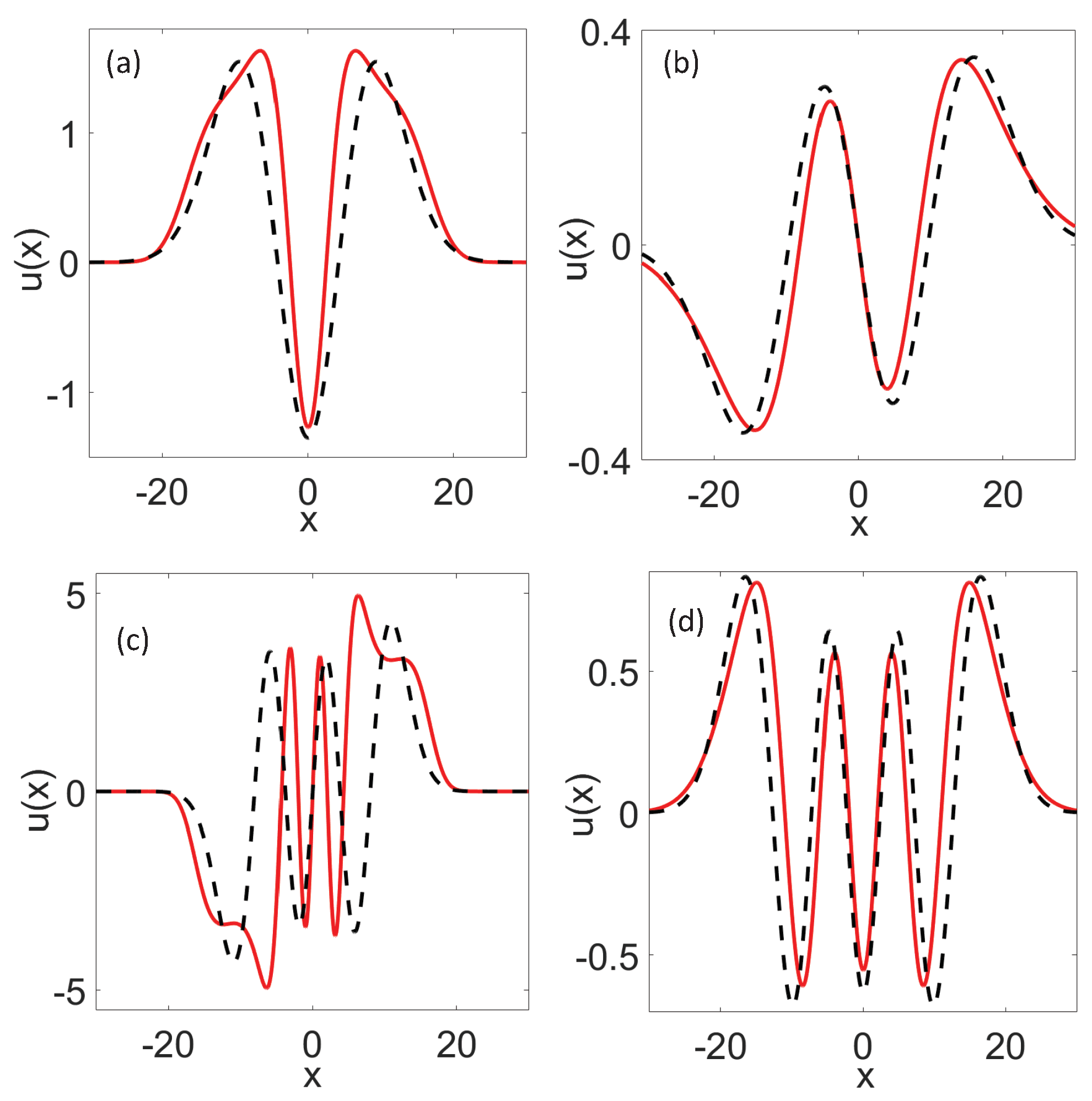
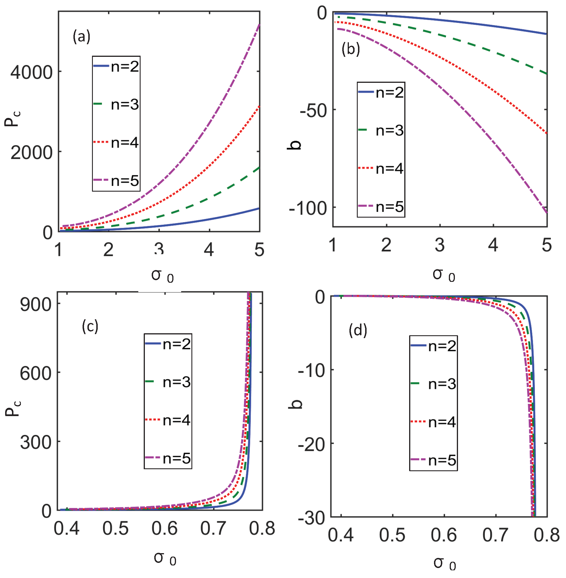
Multipeak solitons can be numerically obtained for two cases of , which are shown in Figure 12 and Figure 13, respectively. Clearly, the multipeak solitons in the case of exhibit Hermite–Gaussian structures and are in good agreement with numerical ones. While, the profiles of solitons in the case of deviate from the Hermite–Gaussian form, especially when becomes large. Likely, for multipeak solitons, the propagation constants and the slope of the power-propagation constant are both negative, which is shown in Figure 14. By linear stability analyses, the ranges of the degree of nonlocality within which the stable multi-peak solitons exist are summarized in Table 2.
5. Perturbation-Iteration Method
In the nonlocally nonlinear system with oscillatory responses governed by Equation (7), the Hermite–Gauss-like solitons with arbitrary peak numbers are hardly obtained by the usual numerical algorithms such as the Newton-conjugate-gradient method. Therefore, we developed a special numerical method by which we called the perturbation-iteration method to solve this problem [38]. The key idea behind the perturbation-iteration method is to treat the NNLSE as a perturbed model of the harmonic oscillator, and soliton solutions can be obtained by perturbation theory in quantum mechanics [46]. The procedure for the perturbation-iteration method is briefly reviewed. Substituting the following soliton solutions:
into the NNLSE (7) yields the following:
where is a coefficient related to the power of soliton, and are, respectively, the transverse distribution and propagation constant of soliton and n is the order of soliton. We can treat Equation (30) as a perturbed model of the harmonic oscillator:
where and are, respectively, eigenfunctions and eigenvalues, is the perturbation compared to the potential of the harmonic oscillator. Starting from the perturbed model of the harmonic oscillator, we determine the “minimum” perturbation, then use the formal expression of infinite-order perturbation expansions to numerically calculate the eigenfunctions and eigenvalues of the perturbed model and iterate this perturbation to obtain multipeak solitons with enough high accuracy.
This form of perturbation-iteration method developed for the -dimensional NNLSE also has been extended to the -case [47]. In fact, the method we developed might also be extended to the numerical integration of the Schrödinger equations in any type of potentials.
6. Optical Beams in NLC with Negative Dielectric Anisotropy
6.1. Evolution Equation for Optical Beams in NLC
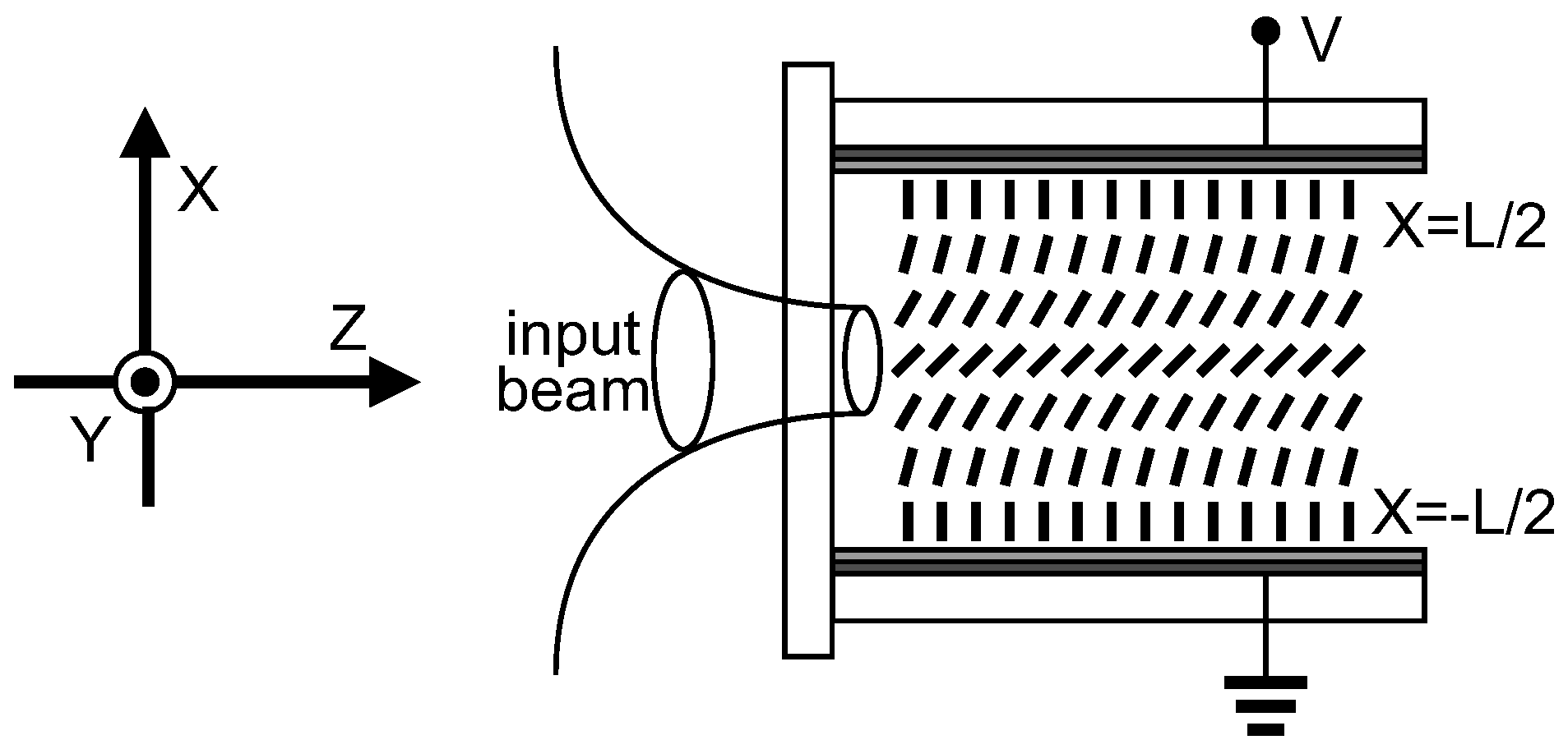
The physical mechanism of nonlinearity in NLC is the optically induced molecular reorientation and nonlocality comes from the interactions between NLC molecules [3]. We consider the propagation of optical beams in the sample cell of NLC shown in Figure 15. NLC molecules exhibit anisotropy in both the low-frequency domain and the optical frequency domain, which is expressed by and , respectively. Anisotropy can be either positive [10,48] or negative [48,49], while is always positive.
When an external low-frequency electrical field and an optical field are present, the molecular director expressed by ( is the tilt angle between and z) will be reorientated. NLC molecules approach the equilibrium state when the three torques are balanced, i.e., , where , and are the optical field-induced torque, low-frequency electrical field induced torque and the elastic torque, respectively. Using the one-constant approximation [48], we can have the following:
where K is the NLC average elastic constant. We can also obtain the following [48]:
where and are the electric displacements, and denotes the time average.
In the absence of light, from the balance of torques of and , the pretilt angle produced by the low-frequency electric field can be determined, which is the only function of X [48]
If (the NLC with positive dielectric anisotropy), , which indicates that the angle at the center () of the cell is at the maximum and decreases as it proceeds closer to the boundaries. The opposite happens for the case that (the NLC with negative dielectric anisotropy), the angle at the center of the cell is at the minimum and increases as it approaches the boundaries. As a result, NLC molecules should be anchored at the boundaries in a manner where for the positive dielectric anisotropy, as was observed in Refs. [3,10,50], and where , as shown in Figure 15, for negative dielectric anisotropy. In addition, the dependence of on low-frequency voltage is different for the NLC with positive and the negative dielectric anisotropy, when is higher than the Fréedericks threshold For the NLC with positive dielectric anisotropy [51], , and for the NLC with negative dielectric anisotropy, we have the following
Although the molecule anchoring at the boundaries is different, the physical processes for both the positive and the negative are the same. Following the procedure to deal with the propagation of optical beams in an NLC with positive dielectric anisotropy [3,10,50], we obtained the equations for that in the NLC with negative dielectric anisotropy and found that the two cases can be uniformly expressed. In the presence of an externally applied (low-frequency) electric field , the propagation of the slowly varying envelope of the optical field linearly polarized along the X-direction (the extraordinary light) and propagating along the Z-direction in the NLC-cell can be described by the following system:
where with being the vacuum wavenumber and being the (linear) refractive index of the extraordinary light. Although it looks the same in form for both cases, Equation (35) is in fact different for either the positive or the negative cases because the sign of is different. The term in Equation (35) was proven to be negligible compared to [50]. Furthermore, we can write , where represents optically induced angle perturbation. By simple substitution into Equation (35), we have the following:
which is the exact result after direct substitution without any approximation. Supposing that the beam width is far smaller than cell thickness L and noting that and in the middle of the cell, we can simplify Equation (36) into the following form:
where we also made sucn an assumption of [3]. Multiplied by , the equation can be re-expressed as follows:
where
are the NRI, the Kerr coefficient and the nonlinear characteristic length for the NLC. When , Equation (38) above will be reduced to for the local limit [39]. Therefore, our definition of in Equation (40) can guarantee that its expression form is consistent when the degree of nonlocality transitions from the nonlocal case to the local case. On the other hand, the propagation equation for optical beams, Equation (34), is simplified as
When , the Kerr coefficient given by Equation (40) is positive, and Equation (38) becomes . This equation is that of the molucular reorientation for NLC with positive dielectric anisotropy and has been discussed extensively [3,10,19,20,50,51,52]. For the NLC with negative dielectric anisotropy, however, , the Kerr coefficient is negative, and Equation (38) becomes , which has been rarely investigated so far. In this case (), by the introduction of the dimensionless transform , , , , and , where , , and is the beam width in Lab coordinate system, Equations (42) and (38) can be transformed as the dimensionless form and , which does be Equations (1) and (2) with .
6.2. Optical Nonlinearities of NLC with Negative Dielectric Anisotropy
By substitution of Equation (33) and , the nonlinear characteristic length given by Equation (41) for the NLC with negative dielectric anisotropy is reduced to the following:
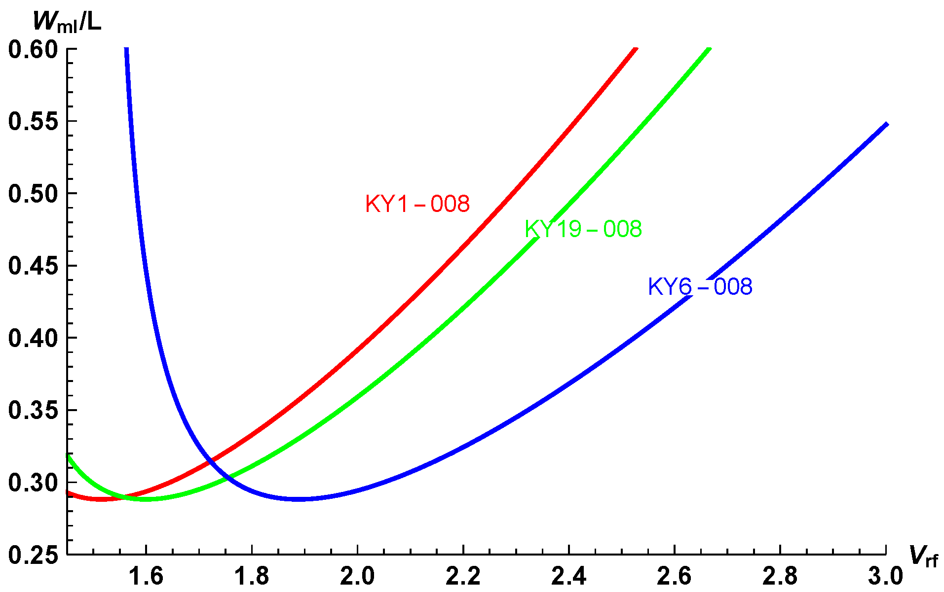
where . is, obviously, the function of the cell thickness L, the bias voltage and the material parameters of the NLC. By setting , we obtain at which takes the minimum , which does not depend on the material parameters of the NLC and is confirmed in Figure 16. Since model Equations (42) and (38) are obtained with the assumption that the beam width in the lab coordinate system, , is far smaller than NLC thickness L, we can assume that so that the weakest degree of nonlocality is , and the degree of nonlocality is always higher than (for an example, for the (1 + 2)-dimensional case). Therefore, the NLC with negative dielectric anisotropy can only behave with self-focusing nonlinearity, and the transition from the self-focusing to the self-defocusing when decreases across the critical point , which was predicted by the system of Equations (1) and (2) with , cannot be observed in the system of Equations (38) and (42) for the negative dielectric anisotropy, because the condition cannot be realized in such a NLC. We also numerically investigated the propagation of the optical beam in the NLC with negative dielectric anisotropy described by Equations (34) and (35) without simplification and found that the beam can always sample the self-focuing nonlinearity indeed [53]. Consequently, the nonlinear refractive index due to reorientation in the pure NLC is always self-focusing, despite the sign of the anisotropy in the low-frequency domain.
It is a well-known fact [54,55,56] that only dark solitons can exist in nonlocally nonlinear media with the positively defining attenuating response and the negative Kerr coefficient () described by Equations (1) and (3) for , no matter how much the degree of nonlocality is. However, as discussed above, the nonlocally nonlinear system of Equations (1) and (2) with , that is, Equations (42) and (38) for the NLC with negative dielectric anisotropy, can exhibit self-focusing nonlinearity in high ranges of the degree of nonlocality and support the bright solitons. It is the unique feature of a nonlocally nonlinear system with oscillatory responses. By the relation of the input optical power between the Lab coordinate system and the dimensionless system
we can have the theoretical value of the critical power via the variational result, i.e., Equation (23) for :
where , and with Ei being the exponential integral function [28]. By using the parameters for the NLC KY19-008 [57], N, , , m, and beam parameters including nm and m, we obtain mW when voltage bias V is applied.
7. Conclusions
We reviewed recent research on the nonlocally nonlinear system with oscillatory responses. This nonlinear system exhibits various new features, such as the nonlocality-controllable transitions of nonlinearities, unique modulational instabilities and new kinds of solitons. The unique features of nonlocally nonlinear system come from oscillatory responses without positive definiteness, which are quite different from the positively defining attenuating ones discussed so far. In particular, in nonlocally nonlinear media with oscillatory responses, we theoretically predicted that bright solitons can exist even when the Kerr coefficient is negative, where only dark solitons were supposed to exist if the response functions are positively defining and attenuating. We find that oscillatory responses can describe the interaction between the optical beam and the nematic liquid crystal with negative dielectric anisotropy, although self-defocusing nonlinearity cannot be exhibited in such a nematic liquid crystal. These new and unexpected behaviors found in the nonlocally nonlinear system with oscillatory responses are of significance at a fundamental level, especially for the relevance between the nonlocality and the focusing-defocusing nonlinearities, which appears to be promising for tailoring optical properties in materials.
Author Contributions
Writing—original draft preparation, writing—review and editing, G.L.; conceptualization, methodology, W.H.; formal analysis, J.L.; conceptualization, methodology, supervision, project administration, Q.G. All authors have read and agreed to the published version of the manuscript.
Funding
This research was supported by the Natural Science Foundation of Guangdong Province of China (No. 2021A1515012214) and the Science and Technology Program of Guangzhou (No. 2019050001).
Acknowledgments
The authors would like to express the thanks to Ying Xiang (Guangdong University of Technology) for his useful and careful discussions on the issues of nematic liquid crystals.
Conflicts of Interest
The authors declare no conflict of interest.
References
- Shen, Y.R. Principles of Nonlinear Optics; Wiley: New York, NY, USA, 1984. [Google Scholar]
- Boyd, R.W. Nonlinear Optics; Academic Press: Amsterdam, The Netherlands, 2008. [Google Scholar]
- Assanto, G. Nematicons: Spatial Optical Solitons in Nematic Liquid Crystals; John Wiley & Sons, Inc.: Hoboken, NJ, USA, 2013. [Google Scholar]
- Snyder, A.W.; Mitchell, D.J. Accessible Solitons. Science 1997, 276, 1538. [Google Scholar] [CrossRef]
- Guo, Q.; Lu, D.; Deng, D. Nonlocal spatial optical solitons. In Advances in Nonlinear Optics; Chen, X., Zhang, G., Zeng, H., Guo, Q., Shen, W., Eds.; De Gruyter: Berlin, Germany, 2015; Chapter 4; pp. 227–305. [Google Scholar]
- Peccianti, M.; Assanto, G. Nematicons. Phys. Rep. 2012, 516, 147. [Google Scholar] [CrossRef]
- Królikowski, W.; Bang, O.; Nikolov, N.I.; Neshev, D.; Wyller, J.; Rasmussen, J.J.; Edmundson, D. Modulational instablity, solitons and beam propagation in spatially nonlocal nonlinear media. J. Opt. B Quantum Semiclass. Opt. 2004, 6, S288. [Google Scholar] [CrossRef] [Green Version]
- Guo, Q. Nonlocal spatial solitons and their interactions. In Optical Transmission, Switching, and Subsystems; SPIE: Bellingham, WA, USA, 2004; Volume 5281, pp. 581–594. [Google Scholar]
- Królikowski, W.; Bang, O.; Briedis, D.; Dreischuh, A.; Edmundson, D.; Luther-Davies, B.; Neshev, D.; Nikolov, N.; Petersen, D.E.; Rasmussen, J.J. Nonlocal solitons. In Nonlinear Optics Applications; SPIE: Warsaw, Poland, 2005; Volume 5949, pp. 76–85. [Google Scholar]
- Conti, C.; Peccianti, M.; Assanto, G. Route to nonlocality and observation of accessible solitons. Phys. Rev. Lett. 2003, 91, 073901. [Google Scholar] [CrossRef] [Green Version]
- Conti, C.; Peccianti, M.; Assanto, G. Observation of optical spatial solitons in a highly nonlocal medium. Phys. Rev. Lett. 2004, 92, 113902. [Google Scholar] [CrossRef]
- Piccardi, A.; Alberucci, A.; Buchnev, O.; Kaczmarek, M.; Khoo, I.C.; Assanto, G. Frequency-controlled deflection of spatial solitons in nematic liquid crystals. Appl. Phys. Lett. 2012, 101, 081112. [Google Scholar] [CrossRef]
- Piccardi, A.; Alberucci, A.; Buchnev, O.; Kaczmarek, M.; Khoo, I.C.; Assanto, G. Frequency-controlled routing of self-confined beams in nematic liquid crystals. Mol. Cryst. Liq. Cryst. 2013, 573, 26. [Google Scholar] [CrossRef]
- Laudyn, U.; Kwasny, M.; Karpierz, M.; Assanto, G. Electro-optic quenching of nematicon fluctuations. Opt. Lett. 2019, 44, 167. [Google Scholar] [CrossRef]
- Rotschild, C.; Cohen, O.; Manela, O.; Segev, M.; Carmon, T. Solitons in nonlinear media with an infinite range of nonlocality: First observation of coherent elliptic solitons and of vortex-ring solitons. Phys. Rev. Lett. 2005, 95, 213904. [Google Scholar] [CrossRef] [Green Version]
- Suter, D.; Blasberg, T. Stabilization of transverse solitary waves by a nonlocal response of the nonlinear medium. Phys. Rev. A 1993, 48, 4583. [Google Scholar] [CrossRef]
- Segev, M.; Crosignani, B.; Yariv, A.; Fischer, B. Spatial solitons in photorefractive media. Phys. Rev. Lett. 1992, 68, 923. [Google Scholar] [CrossRef] [PubMed]
- Parola, A.; Salasnich, L.; Reatto, L. Structure and stability of bosonic clouds: Alkali-metal atoms with negative scattering length. Phys. Rev. A 1998, 57, R3180. [Google Scholar] [CrossRef] [Green Version]
- Rasmussen, P.D.; Bang, O.; Krolikowski, W. Theory of nonlocal soliton interaction in nematic liquid crystals. Phys. Rev. E 2005, 72, 066611. [Google Scholar] [CrossRef] [PubMed] [Green Version]
- Hu, W.; Zhang, T.; Guo, Q.; Xuan, L.; Lan, S. Nonlocality-controlled interaction of spatial solitons in nematic liquid crystals. Appl. Phys. Lett. 2006, 89, 071111. [Google Scholar] [CrossRef] [Green Version]
- Nikolov, N.I.; Neshev, D.; Bang, O.; Krolikowski, W.Z. Quadratic solitons as nonlocal solitons. Phys. Rev. E 2003, 68, 036614. [Google Scholar] [CrossRef] [PubMed] [Green Version]
- Esbensen, B.K.; Bache, M.; Krolikowski, W.; Bang, O. Quadratic solitons for negative effective second-harmonic diffraction as nonlocal solitons with periodic nonlocal response function. Phys. Rev. A 2012, 86, 023849. [Google Scholar] [CrossRef] [Green Version]
- Qin, J.; Dong, G.; Malomed, B.A. Hybrid matter-wave-microwave solitons produced by the local-field effect. Phys. Rev. Lett. 2015, 115, 023901. [Google Scholar] [CrossRef] [Green Version]
- Wang, J.; Li, Y.; Guo, Q.; Hu, W. Stabilization of nonlocal solitons by boundary conditions. Opt. Lett. 2014, 39, 405. [Google Scholar] [CrossRef]
- Wang, J.; Ma, Z.; Li, Y.; Lu, D.; Guo, Q.; Hu, W. Stable quadratic solitons consisting of fundamental waves and oscillatory second harmonics subject to boundary confinement. Phys. Rev. A 2015, 91, 033801. [Google Scholar] [CrossRef]
- Zheng, Y.; Gao, Y.; Wang, J.; Lv, F.; Lu, D.; Hu, W. Bright nonlocal quadratic solitons induced by boundary confinement. Phys. Rev. A 2017, 95, 013808. [Google Scholar] [CrossRef]
- Liang, G.; Hong, W.; Luo, T.; Wang, J.; Li, Y.; Guo, Q.; Hu, W.; Christodoulides, D.N. Transition between self-focusing and self-defocusing in a nonlocally nonlinear system. Phys. Rev. A 2019, 99, 063808. [Google Scholar] [CrossRef] [Green Version]
- Liang, G.; Dang, D.; Li, W.; Li, H.; Guo, Q. Nonlocality-controllable Kerr-nonlinearity in nonlocally nonlinear system with oscillatory responses. New J. Phys. 2020, 22, 073204. [Google Scholar] [CrossRef]
- Liang, G.; Hong, W.; Guo, Q. Spatial solitons with complicated structure in nonlocal nonlinear media. Opt. Express. 2016, 24, 28784. [Google Scholar] [CrossRef] [PubMed]
- Zhong, L.; Dang, D.; Li, W.; Ren, Z.; Guo, Q. Multi-peak solitons in nonlocal nonlinear system with sine-oscillation response. Commun. Nonlinear Sci. 2022, 109, 106322. [Google Scholar] [CrossRef]
- Wang, Z.; Guo, Q.; Hong, W.; Hu, W. Modulational instability in nonlocal Kerr media with a sine-oscillatory response. Opt. Commun. 2017, 394, 31. [Google Scholar] [CrossRef] [Green Version]
- Guan, J.; Ren, Z.; Guo, Q. Stable solution of induced modulation instability. Sci. Rep. 2020, 10, 10081. [Google Scholar] [CrossRef]
- Anderson, D. Variational approach to nonlinear pulse propagation in optical fibers. Phys. Rev. A 1983, 27, 3135. [Google Scholar] [CrossRef]
- Guo, Q.; Luo, B.; Chi, S. Optical beams in sub-strongly non-local nonlinear media: A variational solution. Opt. Commun. 2006, 259, 336. [Google Scholar] [CrossRef]
- Haus, H.A. Waves and Fields in Optoelectronics; Prentice-Hall: Englewood Cliffs, NJ, USA, 1984. [Google Scholar]
- Agrawal, G.P. Nonlinear Fiber Optics, 4th ed.; Academic: San Diego, CA, USA, 2007. [Google Scholar]
- Hu, Y.; Lou, S. Analytical descriptions of dark and gray solitons in nonlocal nonlinear media. Commun. Theor. Phys. 2015, 64, 665. [Google Scholar] [CrossRef]
- Hong, W.; Tian, B.; Li, R.; Guo, Q.; Hu, W. Perturbation-iteration method for multi-peak solitons in nonlocal nonlinear media. J. Opt. Soc. Am. B 2018, 35, 317. [Google Scholar] [CrossRef] [Green Version]
- Kivshar, Y.S.; Agrawal, G.P. Optical Solitons: From Fibers to Photonic Crystals; Academic Press Inc.: Cambridge, MA, USA, 2003. [Google Scholar]
- Sakaguchi, H.; Malomed, B.A. Solitons in combined linear and nonlinear lattice potentials. Phys. Rev. A 2010, 81, 013624. [Google Scholar] [CrossRef] [Green Version]
- Qin, J.; Dong, G.; Malomed, B.A. Stable giant vortex annuli in microwave-coupled atomic condensates. Phys. Rev. A 2016, 94, 053611. [Google Scholar] [CrossRef] [Green Version]
- Qin, J.; Liang, Z.; Malomed, B.A.; Dong, G. Tail-free self-accelerating solitons and vortices. Phys. Rev. A 2019, 99, 023610. [Google Scholar] [CrossRef] [Green Version]
- Buryak, A.V.; Kivshar, Y.S. Solitons due to second harmonic generation. Phys. Lett. A 1995, 197, 407. [Google Scholar] [CrossRef]
- Xu, Z.; Kartashov, Y.V.; Torner, L. Upper threshold for stability of multipole-mode solitons in nonlocal nonlinear media. Opt. Lett. 2005, 30, 3171. [Google Scholar] [CrossRef] [Green Version]
- Dong, L.; Ye, F. Stability of multipole-mode solitons in thermal nonlinear media. Phys. Rev. A 2010, 81, 013815. [Google Scholar] [CrossRef] [Green Version]
- Ouyang, S.; Guo, Q.; Hu, W. Perturbative analysis of generally nonlocal spatial optical solitons. Phys. Rev. E 2006, 74, 036622. [Google Scholar] [CrossRef] [Green Version]
- Tian, B.; Guo, Q.; Hong, W.; Hu, W. Extension of the perturbation-iteration method to (1 + 2)-dimensional case. Optik 2019, 192, 162909. [Google Scholar] [CrossRef]
- Khoo, I.C. Liquid Crystals: Physical Properties and Nonlinear Optical Phenomena; Wiley: New York, NY, USA, 1995. [Google Scholar]
- Schiekel, M.F.; Fahrenschon, K. Deformation of nematic liquid crystals with vertical orientation in electrical fields. Appl. Phys. Lett. 1971, 19, 391. [Google Scholar] [CrossRef]
- Peccianti, M.; Conti, C.; Assanto, G.; De Luca, A.; Umeton, C. Nonlocal optical propagation in nonlinear nematic liquid crystals. J. Nonlinear Opt. Phys. Mater. 2003, 12, 525. [Google Scholar] [CrossRef]
- Peccianti, M.; Conti, C.; Assanto, G. Interplay between nonlocality and nonlinearity in nematic liquid crystals. Opt. Lett. 2005, 30, 415. [Google Scholar] [CrossRef] [PubMed]
- Assanto, G.; Peccianti, M. Spatial solitons in Nematic liquid crystals. IEEE J. Quantum Electron. 2003, 39, 13. [Google Scholar] [CrossRef]
- Zhang, Y. Numerical Research on Modulation Instability of Nematic Liquid Crystals with Negative Dielectric Anisotropy. Master’s Dissertation, South China Normal University, Guangzhou, China, 2005. (In Chinese). [Google Scholar]
- Krolikowski, W.; Bang, O. Solitons in nonlocal nonlinear media: Exact solutions. Phys. Rev. E 2000, 63, 016610. [Google Scholar] [CrossRef] [Green Version]
- Kong, Q.; Wang, Q.; Bang, O.; Krolikowski, W. Analytical theory of dark nonlocal solitons. Opt. Lett. 2010, 35, 2152. [Google Scholar] [CrossRef] [PubMed] [Green Version]
- Conti, C.; Fratalocchi, A.; Peccianti, M.; Ruocco, G.; Trillo, S. Observation of a gradient catastrophe generating solitons. Phys. Rev. Lett. 2009, 102, 083902. [Google Scholar] [CrossRef] [PubMed] [Green Version]
- Wang, J.; Chen, J.; Liu, J.; Li, Y.; Guo, Q.; Hu, W.; Xuan, L. Nematicons in liquid crystals with negative dielectric anisotropy. arXiv 2018, arXiv:1403.2154v2. [Google Scholar]
Figure 1.
Critical degree of nonlocality as the function of propagation distance z. (a) , (b) . All data of the curves are numerically obtained from Equation (12) (After Ref. [28]).

Figure 2.
Beam widths at as the function of for different input powers. (a) , (b) . Solid color curves represent the numerical simulation results, agreeing well with the variational results denoted by dashed color curves. For comparison, the output beam width at in the linear case is also plotted by the horizontal solid straight line (After Ref. [28]).

Figure 3.
Evolutions of optical beams for both (,) and (,). in (,), whereas in (,). The linear evolutions are displayed in (,) for comparison (After Ref. [27]).
Figure 3.
Evolutions of optical beams for both (,) and (,). in (,), whereas in (,). The linear evolutions are displayed in (,) for comparison (After Ref. [27]).

Figure 4.
Gain spectra of MI under different values of when .

Figure 5.
Gain spectra of MI under different values of when .

Figure 6.
Evolution of the optical field at under input condition (19) when (solid line: analytical results obtained through linear approximation method; dashed line: results attained through simulation) (After Ref. [32]).

Figure 7.
Evolution of stable solution when at different modulation frequencies: (a) ; (b) (After Ref. [32]).
Figure 7.
Evolution of stable solution when at different modulation frequencies: (a) ; (b) (After Ref. [32]).

Figure 8.
Critical power and the soliton propagation constant versus the degree of nonlocality . The inset shows versus . All plots are for . The obtained solitons are stable (After Ref. [27]).
Figure 8.
Critical power and the soliton propagation constant versus the degree of nonlocality . The inset shows versus . All plots are for . The obtained solitons are stable (After Ref. [27]).

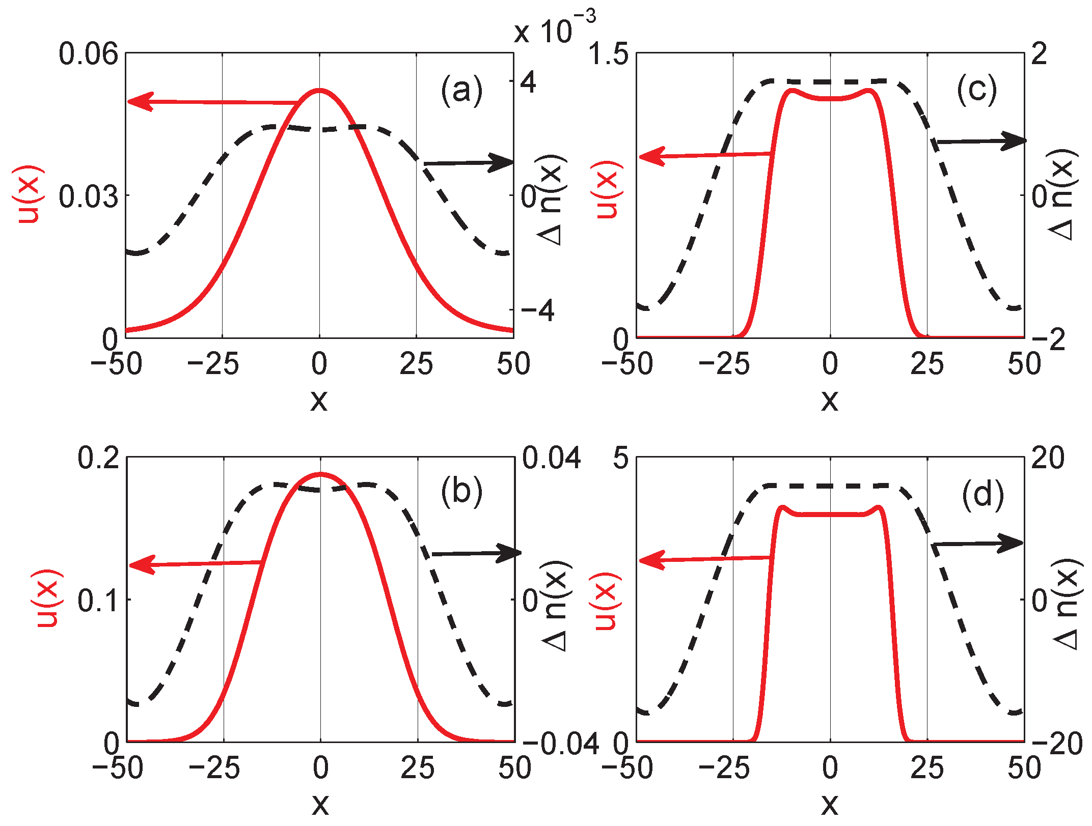
Figure 9.
Profiles of in-phase bound-state solitons (solid red lines) and their induced NRI (dashed black lines) for the case that . (a) , (b) , (c) and (d) . The obtained solitons are stable (After Ref. [29]).
Figure 9.
Profiles of in-phase bound-state solitons (solid red lines) and their induced NRI (dashed black lines) for the case that . (a) , (b) , (c) and (d) . The obtained solitons are stable (After Ref. [29]).

Figure 10.
Profile of out-of-phase bound-state solitons (solid red lines) and the induced NRI (dashed black lines) for the case that . (a) , (b) , (c) and (d) . The obtained solitons are stable (After Ref. [29]).
Figure 10.
Profile of out-of-phase bound-state solitons (solid red lines) and the induced NRI (dashed black lines) for the case that . (a) , (b) , (c) and (d) . The obtained solitons are stable (After Ref. [29]).

Figure 11.
(a) Power P and propagation constant vs. the degree of nonlocality ; (b) power P vs. propagation constant of the in-phase and out-of-phase bound-state solitons for the case that . The obtained solitons are stable (After Ref. [29]).
Figure 11.
(a) Power P and propagation constant vs. the degree of nonlocality ; (b) power P vs. propagation constant of the in-phase and out-of-phase bound-state solitons for the case that . The obtained solitons are stable (After Ref. [29]).

Figure 12.
Profiles of the numerical multi–peak solitons (the solid red curves) for and . (a–d) for and , respectively. The variational results (the dashed black curves) with the same parameters are also given for comparison. Soliton in (b) is stable, while the ones in the other three figures are unstable.

Figure 13.
Profiles of the numerical multi–peak solitons (the solid red curves) for and . (a–d) for and , respectively. The corresponding numerical results are denoted in the same manner as in Figure 5. Soliton in (b) is stable, while the ones in the other three figures are unstable.
Figure 13.
Profiles of the numerical multi–peak solitons (the solid red curves) for and . (a–d) for and , respectively. The corresponding numerical results are denoted in the same manner as in Figure 5. Soliton in (b) is stable, while the ones in the other three figures are unstable.

Figure 14.
Dependencies of the power on the degree of nonlocality (a,c) and the propagation constant b on the degree of nonlocality (b,d) for the multi–peak solitons. (a,b) and (c,d) for and , respectively.)
Figure 14.
Dependencies of the power on the degree of nonlocality (a,c) and the propagation constant b on the degree of nonlocality (b,d) for the multi–peak solitons. (a,b) and (c,d) for and , respectively.)

Figure 15.
X-Z cross-section of the planar cell of the NLC with negative dielectric anisotropy, and the cell can be considered invariant along Y. Two pieces of glasses sandwiches NLC. Polymer coatings provide molecules anchoring at the boundaries, and ITO films allow for the application of low frequency bias. An optical beam propagating inside the cell along Z induces an index perturbation.

Figure 16.
Dependence of on bias voltage for different NLC samples. The values of are , and for KY1-008, KY19-008 and KY6-008-type NLCs, respectively. for all materials.
Figure 16.
Dependence of on bias voltage for different NLC samples. The values of are , and for KY1-008, KY19-008 and KY6-008-type NLCs, respectively. for all materials.


Table 1.
The ranges of within which the HG-type solitons exist.
| variational | |||||
| numerical | |||||
| variational | |||||
| numerical |
Note: self-focusing nonlinearity is exhibited when σ0 ∈ (σc, +∞) for s = −1, and [0, σc] for s = 1 (for example, = 0.82.)
Table 2.
The ranges of within which the HG–type solitons are stable.
| no | ||||||
| no | no |
Publisher’s Note: MDPI stays neutral with regard to jurisdictional claims in published maps and institutional affiliations. |
© 2022 by the authors. Licensee MDPI, Basel, Switzerland. This article is an open access article distributed under the terms and conditions of the Creative Commons Attribution (CC BY) license (https://creativecommons.org/licenses/by/4.0/).
Share and Cite
MDPI and ACS Style
Liang, G.; Liu, J.; Hu, W.; Guo, Q. Unique Features of Nonlocally Nonlinear Systems with Oscillatory Responses. Appl. Sci. 2022, 12, 2386. https://doi.org/10.3390/app12052386
AMA Style
Liang G, Liu J, Hu W, Guo Q. Unique Features of Nonlocally Nonlinear Systems with Oscillatory Responses. Applied Sciences. 2022; 12(5):2386. https://doi.org/10.3390/app12052386
Chicago/Turabian StyleLiang, Guo, Jinlong Liu, Wei Hu, and Qi Guo. 2022. "Unique Features of Nonlocally Nonlinear Systems with Oscillatory Responses" Applied Sciences 12, no. 5: 2386. https://doi.org/10.3390/app12052386
Note that from the first issue of 2016, this journal uses article numbers instead of page numbers. See further details here.