
Deep Learning-Based In Vitro Detection Method for Cellular Impurities in Human Cell-Processed Therapeutic Products

 , and
, and
Abstract
:Featured Application
Abstract
1. Introduction
2. Materials and Methods
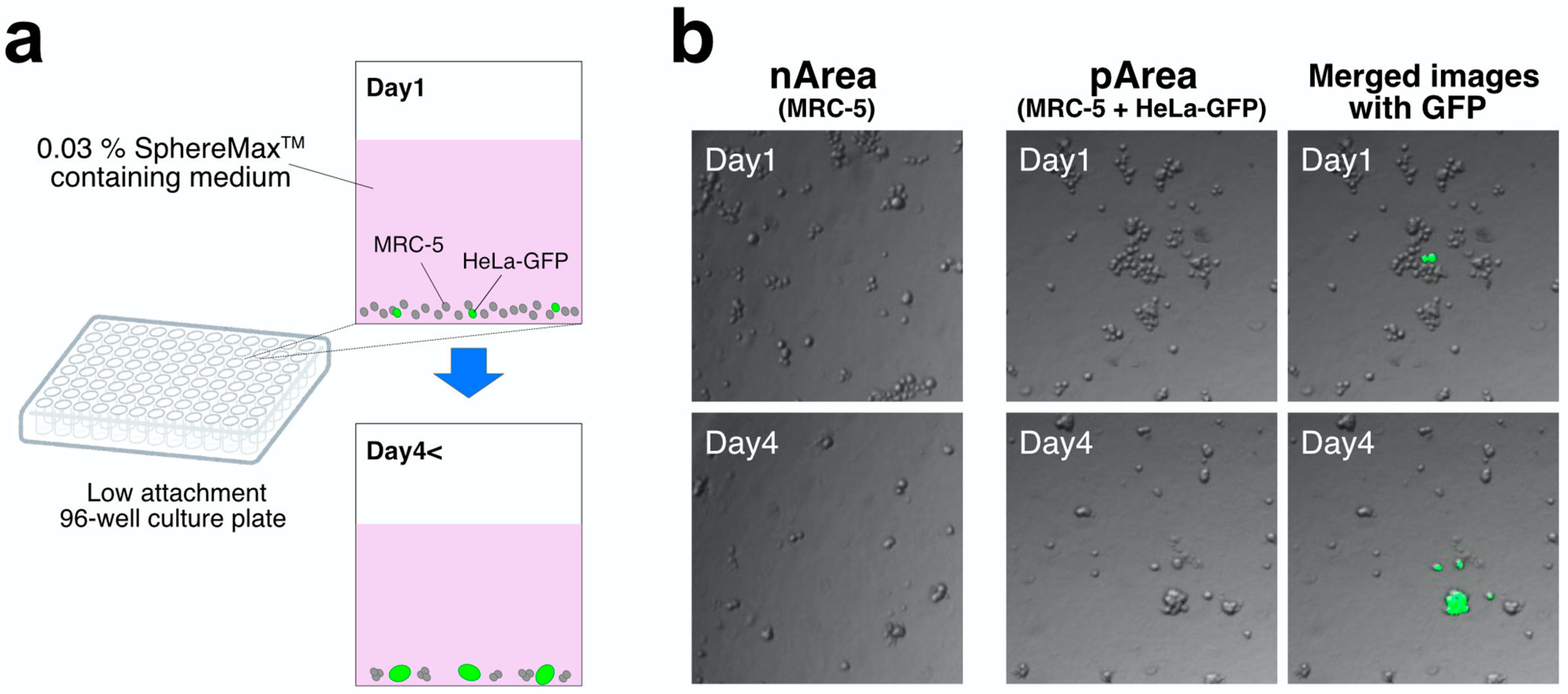
2.1. Cell Culture System
2.2. Preparation of the Image Data of Culture Cells
2.3. Deep Learning
3. Results
4. Discussion
- (1)
- Low-degree polynomial models: any polynomial can be approximated by a neural network consisting of about four times as many neurons as the number of multiplications required for calculation.
- (2)
- Locality: a local Markov network can be approximated using a neural network consisting of a number of neurons proportional to the number of nodes.
- (3)
- Symmetry: CNNs that explicitly incorporate mobile and temporal universality can significantly reduce the number of parameters required for learning, which also greatly reduces the apparent complexity [74].
- (1)
- Increase the number of training data
- (2)
- Model simplification
- (3)
- Regularization
- (1)
- Support vector machine (SVM)
- (2)
- K-nearest neighbor (kNN) algorithm
- (3)
- Naïve Bayes classifier
5. Conclusions
Supplementary Materials
Author Contributions
Funding
Institutional Review Board Statement
Informed Consent Statement
Data Availability Statement
Acknowledgments
Conflicts of Interest
References
- Yasuda, S.; Sato, Y. Tumorigenicity assessment of human cell-processed therapeutic products. Biologicals 2015, 43, 416–421. [Google Scholar] [CrossRef] [PubMed]
- Kono, K.; Sawada, R.; Kuroda, T.; Yasuda, S.; Matsuyama, S.; Matsuyama, A.; Mizuguchi, H.; Sato, Y. Development of selective cytotoxic viral vectors for concentration of undifferentiated cells in cardiomyocytes derived from human induced pluripotent stem cells. Sci. Rep. 2019, 9, 3630. [Google Scholar] [CrossRef] [Green Version]
- Gao, Y.; Pu, J. Differentiation and application of human pluripotent stem cells derived cardiovascular cells for treatment of heart diseases: Promises and challenges. Front. Cell Dev. Biol. 2021, 9, 658088. [Google Scholar] [CrossRef]
- McGarvey, S.S.; Ferreyros, M.; Kogut, I.; Bilousova, G. Differentiating induced pluripotent stem cells toward mesenchymal stem/stromal cells. Methods Mol. Biol. 2021, in press. [Google Scholar] [CrossRef]
- Theopold, C.; Hoeller, D.; Velander, P.; Demling, R.; Eriksson, E. Graft site malignancy following treatment of full-thickness burn with cultured epidermal autograft. Plast. Reconstr. Surg. 2004, 114, 1215–1219. [Google Scholar] [CrossRef]
- Amariglio, N.; Hirshberg, A.; Scheithauer, B.W.; Cohen, Y.; Loewenthal, R.; Trakhtenbrot, L.; Paz, N.; Koren-Michowitz, M.; Waldman, D.; Leider-Trejo, L.; et al. Donor-derived brain tumor following neural stem cell transplantation in an ataxia telangiectasia patient. PLoS Med. 2009, 6, e1000029. [Google Scholar] [CrossRef]
- Ben-David, U.; Benvenisty, N. The tumorigenicity of human embryonic and induced pluripotent stem cells. Nat. Rev. Cancer 2011, 11, 268–277. [Google Scholar] [CrossRef]
- Dlouhy, B.J.; Awe, O.; Rao, R.C.; Kirby, P.A.; Hitchon, P.W. Autograft-derived spinal cord mass following olfactory mucosal cell transplantation in a spinal cord injury patient: Case report. J. Neurosurg. Spine 2014, 21, 618–622. [Google Scholar] [CrossRef] [PubMed] [Green Version]
- Kusakawa, S.; Machida, K.; Yasuda, S.; Takada, N.; Kuroda, T.; Sawada, R.; Okura, H.; Tsutsumi, H.; Kawamata, S.; Sato, Y. Characterization of in vivo tumorigenicity tests using severe immunodeficient NOD/Shi-scid IL2Rgamma(null) mice for detection of tumorigenic cellular impurities in human cell-processed therapeutic products. Regen. Ther. 2015, 1, 30–37. [Google Scholar] [CrossRef] [Green Version]
- Kusakawa, S.; Yasuda, S.; Kuroda, T.; Kawamata, S.; Sato, Y. Ultra-sensitive detection of tumorigenic cellular impurities in human cell-processed therapeutic products by digital analysis of soft agar colony formation. Sci. Rep. 2015, 5, 17892. [Google Scholar] [CrossRef] [Green Version]
- Hasebe-Takada, N.; Kono, K.; Yasuda, S.; Sawada, R.; Matsuyama, A.; Sato, Y. Application of cell growth analysis to the quality assessment of human cell-processed therapeutic products as a testing method for immortalized cellular impurities. Regen. Ther. 2016, 5, 49–54. [Google Scholar] [CrossRef] [Green Version]
- Lee, B.; Borys, B.S.; Kallos, M.S.; Rodrigues, C.A.V.; Silva, T.P.; Cabral, J.M.S. Challenges and solutions for commercial scale manufacturing of allogeneic pluripotent stem cell products. Bioengineering. 2020, 7, 31. [Google Scholar] [CrossRef] [PubMed] [Green Version]
- Qiao, Y.; Agboola, O.S.; Hu, X.; Wu, Y.; Lei, L. Tumorigenic and immunogenic properties of induced pluripotent stem cells: A promising cancer vaccine. Stem Cell Rev. Rep. 2020, 16, 1049–1061. [Google Scholar] [CrossRef] [PubMed]
- Johnson, D.L.; Scott, R.; Newman, R. Pluripotent stem cell culture scale-out. In Assay Guidance Manual; Markossian, S., Grossman, A., Brimacombe, K., Arkin, M., Auld, D., Austin, C.P., Baell, J., Chung, T.D.Y., Coussens, N.P., Dahlin, J.L., et al., Eds.; Eli Lilly & Company and the National Center for Advancing Translational Sciences: Bethesda, MD, USA, 2021. [Google Scholar]
- Radrizzani, M.; Soncin, S.; Bolis, S.; Lo Cicero, V.; Andriolo, G.; Turchetto, L. Quality control assays for clinical-grade human mesenchymal stromal cells: Validation strategy. Methods Mol. Biol. 2016, 1416, 339–356. [Google Scholar] [CrossRef]
- Radrizzani, M.; Soncin, S.; Lo Cicero, V.; Andriolo, G.; Bolis, S.; Turchetto, L. Quality control assays for clinical-grade human mesenchymal stromal cells: Methods for ATMP release. Methods Mol. Biol. 2016, 1416, 313–337. [Google Scholar] [CrossRef] [PubMed]
- Nath, S.C.; Harper, L.; Rancourt, D.E. Cell-based therapy manufacturing in stirred suspension bioreactor: Thoughts for cGMP compliance. Front. Bioeng. Biotechnol. 2020, 8, 599674. [Google Scholar] [CrossRef] [PubMed]
- Kilic, P. Quality Management Systems (QMSs) of human-based tissue and cell product manufacturing facilities. Methods Mol. Biol. 2021, 2286, 263–279. [Google Scholar] [CrossRef]
- Kusena, J.W.T.; Shariatzadeh, M.; Thomas, R.J.; Wilson, S.L. Understanding cell culture dynamics: A tool for defining protocol parameters for improved processes and efficient manufacturing using human embryonic stem cells. Bioengineered 2021, 12, 979–996. [Google Scholar] [CrossRef]
- Tigges, J.; Bielec, K.; Brockerhoff, G.; Hildebrandt, B.; Hübenthal, U.; Kapr, J.; Koch, K.; Teichweyde, N.; Wieczorek, D.; Rossi, A.; et al. Academic application of good cell culture practice for induced pluripotent stem cells. Altern. Anim. Exp. 2021, in press. [Google Scholar] [CrossRef]
- Wang, Y.; Huso, D.L.; Harrington, J.; Kellner, J.; Jeong, D.K.; Turney, J.; McNiece, I.K. Outgrowth of a transformed cell population derived from normal human BM mesenchymal stem cell culture. Cytotherapy 2005, 7, 509–519. [Google Scholar] [CrossRef]
- Yang, S.; Lin, G.; Tan, Y.Q.; Zhou, D.; Deng, L.Y.; Cheng, D.H.; Luo, S.W.; Liu, T.C.; Zhou, X.Y.; Sun, Z.; et al. Tumor progression of culture-adapted human embryonic stem cells during long-term culture. Genes Chromosomes Cancer 2008, 47, 665–679. [Google Scholar] [CrossRef] [PubMed]
- Røsland, G.V.; Svendsen, A.; Torsvik, A.; Sobala, E.; McCormack, E.; Immervoll, H.; Mysliwietz, J.; Tonn, J.C.; Goldbrunner, R.; Lønning, P.E.; et al. Long-term cultures of bone marrow-derived human mesenchymal stem cells frequently undergo spontaneous malignant transformation. Cancer Res. 2009, 69, 5331–5339. [Google Scholar] [CrossRef] [Green Version]
- Garcia, S.; Bernad, A.; Martín, M.C.; Cigudosa, J.C.; Garcia-Castro, J.; de la Fuente, R. Pitfalls in spontaneous in vitro transformation of human mesenchymal stem cells. Exp. Cell Res. 2010, 316, 1648–1650. [Google Scholar] [CrossRef] [PubMed]
- Capes-Davis, A.; Theodosopoulos, G.; Atkin, I.; Drexler, H.G.; Kohara, A.; MacLeod, R.A.; Masters, J.R.; Nakamura, Y.; Reid, Y.A.; Reddel, R.R.; et al. Check your cultures! A list of cross-contaminated or misidentified cell lines. Int. J. Cancer 2010, 127, 1–8. [Google Scholar] [CrossRef]
- Torsvik, A.; Røsland, G.V.; Svendsen, A.; Molven, A.; Immervoll, H.; McCormack, E.; Lønning, P.E.; Primon, M.; Sobala, E.; Tonn, J.C.; et al. Spontaneous malignant transformation of human mesenchymal stem cells reflects cross-contamination: Putting the research field on track-letter. Cancer Res. 2010, 70, 6393–6396. [Google Scholar] [CrossRef] [Green Version]
- Tang, D.Q.; Wang, Q.; Burkhardt, B.R.; Litherland, S.A.; Atkinson, M.A.; Yang, L.J. In vitro generation of functional insulin-producing cells from human bone marrow-derived stem cells, but long-term culture running risk of malignant transformation. Am. J. Stem Cells 2012, 1, 114–127. [Google Scholar]
- Horbach, S.P.J.M.; Halffman, W. The ghosts of HeLa: How cell line misidentification contaminates the scientific literature. PLoS ONE 2017, 12, e0186281. [Google Scholar] [CrossRef]
- Lin, L.C.; Elkashty, O.; Ramamoorthi, M.; Trinh, N.; Liu, Y.; Sunavala-Dossabhoy, G.; Pranzatelli, T.; Michael, D.G.; Chivasso, C.; Perret, J.; et al. Cross-contamination of the human salivary gland HSG cell line with HeLa cells: A STR analysis study. Oral Dis. 2018, 24, 1477–1483. [Google Scholar] [CrossRef]
- Liu, J.; Zeng, S.; Wang, Y.; Yu, J.; Ouyang, Q.; Hu, L.; Zhou, D.; Lin, G.; Sun, Y. Essentiality of CTNNB1 in malignant transformation of human embryonic stem cells under long-term suboptimal conditions. Stem Cells Int. 2020, 2020, 5823676. [Google Scholar] [CrossRef] [PubMed]
- Wang, R.; Wang, D.; Kang, D.; Guo, X.; Guo, C.; Dongye, M.; Zhu, Y.; Chen, C.; Zhang, X.; Long, E.; et al. An artificial intelligent platform for live cell identification and the detection of cross-contamination. Ann. Transl. Med. 2020, 8, 697. [Google Scholar] [CrossRef]
- Yasuda, S.; Kusakawa, S.; Kuroda, T.; Miura, T.; Tano, K.; Takada, N.; Matsuyama, S.; Matsuyama, A.; Nasu, M.; Umezawa, A.; et al. Tumorigenicity-associated characteristics of human iPS cell lines. PLoS ONE 2018, 13, e0205022. [Google Scholar] [CrossRef] [Green Version]
- Luijten, M.; Corvi, R.; Mehta, J.; Corvaro, M.; Delrue, N.; Felter, S.; Haas, B.; Hewitt, N.J.; Hilton, G.; Holmes, T.; et al. A comprehensive view on mechanistic approaches for cancer risk assessment of non-genotoxic agrochemicals. Regul. Toxicol. Pharmacol. 2020, 118, 104789. [Google Scholar] [CrossRef]
- Chour, T.; Tian, L.; Lau, E.; Thomas, D.; Itzhaki, I.; Malak, O.; Zhang, J.Z.; Qin, X.; Wardak, M.; Liu, Y.; et al. Method for selective ablation of undifferentiated human pluripotent stem cell populations for cell-based therapies. JCI Insight 2021, 6, e142000. [Google Scholar] [CrossRef]
- Held, M.; Schmitz, M.H.; Fischer, B.; Walter, T.; Neumann, B.; Olma, M.H.; Peter, M.; Ellenberg, J.; Gerlich, D.W. CellCognition: Time-resolved phenotype annotation in high-throughput live cell imaging. Nat. Methods 2010, 7, 747–754. [Google Scholar] [CrossRef] [Green Version]
- Buggenthin, F.; Buettner, F.; Hoppe, P.S.; Endele, M.; Kroiss, M.; Strasser, M.; Schwarzfischer, M.; Loeffler, D.; Kokkaliaris, K.D.; Hilsenbeck, O.; et al. Prospective identification of hematopoietic lineage choice by deep learning. Nat. Methods 2017, 14, 403–406. [Google Scholar] [CrossRef]
- Niioka, H.; Asatani, S.; Yoshimura, A.; Ohigashi, H.; Tagawa, S.; Miyake, J. Classification of C2C12 cells at differentiation by convolutional neural network of deep learning using phase contrast images. Hum. Cell 2018, 31, 87–93. [Google Scholar] [CrossRef] [Green Version]
- Yao, K.; Rochman, N.D.; Sun, S.X. Cell type classification and unsupervised morphological phenotyping from low-resolution images using deep learning. Sci. Rep. 2019, 9, 13467. [Google Scholar] [CrossRef] [PubMed] [Green Version]
- Maruthamuthu, M.K.; Raffiee, A.H.; De Oliveira, D.M.; Ardekani, A.M.; Verma, M.S. Raman spectra-based deep learning: A tool to identify microbial contamination. Microbiologyopen 2020, 9, e1122. [Google Scholar] [CrossRef] [PubMed]
- Mzurikwao, D.; Khan, M.U.; Samuel, O.W.; Cinatl, J., Jr.; Wass, M.; Michaelis, M.; Marcelli, G.; Ang, C.S. Towards image-based cancer cell lines authentication using deep neural networks. Sci. Rep. 2020, 10, 19857. [Google Scholar] [CrossRef] [PubMed]
- Chen, X.; Li, Y.; Wyman, N.; Zhang, Z.; Fan, H.; Le, M.; Gannon, S.; Rose, C.; Zhang, Z.; Mercuri, J.; et al. Deep learning provides high accuracy in automated chondrocyte viability assessment in articular cartilage using nonlinear optical microscopy. Biomed. Opt. Express 2021, 12, 2759–2772. [Google Scholar] [CrossRef] [PubMed]
- Hu, H.; Liu, A.; Zhou, Q.; Guan, Q.; Li, X.; Chen, Q. An adaptive learning method of anchor shape priors for biological cells detection and segmentation. Comput. Methods Programs Biomed. 2021, 208, 106260. [Google Scholar] [CrossRef]
- Iseoka, H.; Sasai, M.; Miyagawa, S.; Takekita, K.; Date, S.; Ayame, H.; Nishida, A.; Sanami, S.; Hayakawa, T.; Sawa, Y. Rapid and sensitive mycoplasma detection system using image-based deep learning. J. Artif. Organs 2021, in press. [Google Scholar] [CrossRef]
- Theriault, D.H.; Walker, M.L.; Wong, J.Y.; Betke, M. Cell morphology classification and clutter mitigation in phase-contrast microscopy images using machine learning. Mach. Vis. Appl. 2012, 23, 659–673. [Google Scholar] [CrossRef]
- Matsuoka, F.; Takeuchi, I.; Agata, H.; Kagami, H.; Shiono, H.; Kiyota, Y.; Honda, H.; Kato, R. Morphology-based prediction of osteogenic differentiation potential of human mesenchymal stem cells. PLoS ONE 2013, 8, e55082. [Google Scholar] [CrossRef]
- Tokunaga, K.; Saitoh, N.; Goldberg, I.G.; Sakamoto, C.; Yasuda, Y.; Yoshida, Y.; Yamanaka, S.; Nakao, M. Computational image analysis of colony and nuclear morphology to evaluate human induced pluripotent stem cells. Sci. Rep. 2014, 4, 6996. [Google Scholar] [CrossRef] [Green Version]
- Sasaki, K.; Sasaki, H.; Takahashi, A.; Kang, S.; Yuasa, T.; Kato, R. Non-invasive quality evaluation of confluent cells by image-based orientation heterogeneity analysis. J. Biosci. Bioeng. 2016, 121, 227–234. [Google Scholar] [CrossRef] [PubMed]
- Boumaraf, S.; Liu, X.; Wan, Y.; Zheng, Z.; Ferkous, C.; Ma, X.; Li, Z.; Bardou, D. Conventional machine learning versus deep learning for magnification Dependent histopathological breast cancer image classification: A comparative study with visual explanation. Diagnostics. 2021, 11, 528. [Google Scholar] [CrossRef]
- Shoeibi, A.; Khodatars, M.; Jafari, M.; Moridian, P.; Rezaei, M.; Alizadehsani, R.; Khozeimeh, F.; Gorriz, J.M.; Heras, J.; Panahiazar, M.; et al. Applications of deep learning techniques for automated multiple sclerosis detection using magnetic resonance imaging: A review. Comput. Biol. Med. 2021, 136, 104697. [Google Scholar] [CrossRef] [PubMed]
- Van Valen, D.A.; Kudo, T.; Lane, K.M.; Macklin, D.N.; Quach, N.T.; DeFelice, M.M.; Maayan, I.; Tanouchi, Y.; Ashley, E.A.; Covert, M.W. Deep learning automates the quantitative analysis of individual cells in live-cell imaging experiments. PLoS Comput. Biol. 2016, 12, e1005177. [Google Scholar] [CrossRef] [Green Version]
- Chang, Y.-H.; Abe, K.; Yokota, H.; Sudo, K.; Nakamura, Y.; Lin, C.-T.; Tsai, M.-D. Human induced pluripotent stem cell region recognition in microscopy images using Convolutional Neural Networks. In Proceedings of the 39th Annual International Conference of the IEEE Engineering in Medicine and Biology Society (EMBC), Jeju, Korea, 11–15 July 2017; pp. 4058–4061. [Google Scholar] [CrossRef]
- Hong, J.; Park, B.-Y.; Park, H. Convolutional neural network classifier for distinguishing Barrett’s esophagus and neoplasia endomicroscopy images. In Proceedings of the 39th Annual International Conference of the IEEE Engineering in Medicine and Biology Society (EMBC), Jeju, Korea, 11–15 July 2017; pp. 2892–2895. [Google Scholar] [CrossRef]
- Toratani, M.; Konno, M.; Asai, A.; Koseki, J.; Kawamoto, K.; Tamari, K.; Li, Z.; Sakai, D.; Kudo, T.; Satoh, T.; et al. A convolutional neural network uses microscopic images to differentiate between mouse and human cell lines and their radioresistant clones. Cancer Res. 2018, 78, 6703–6707. [Google Scholar] [CrossRef] [Green Version]
- Guo, X.; Wang, F.; Teodoro, G.; Farris, A.B.; Kong, J. Liver steatosis segmentation with deep learning methods. In Proceedings of the 16th IEEE International Symposium on Biomedical Imaging (ISBI 2019), Venice, Italy, 8–11 April 2019; pp. 24–27. [Google Scholar] [CrossRef] [Green Version]
- Orita, K.; Sawada, K.; Koyama, R.; Ikegaya, Y. Deep learning-based quality control of cultured human-induced pluripotent stem cell-derived cardiomyocytes. J. Pharmacol. Sci. 2019, 140, 313–316. [Google Scholar] [CrossRef] [PubMed]
- Thillaikkarasi, R.; Saravanan, S. An enhancement of deep learning algorithm for brain tumor segmentation using Kernel based CNN with M-SVM. J. Med. Syst. 2019, 43, 84. [Google Scholar] [CrossRef]
- Lin, Y.H.; Liao, K.Y.; Sung, K.B. Automatic detection and characterization of quantitative phase images of thalassemic red blood cells using a mask region-based convolutional neural network. J. Biomed. Opt. 2020, 25, 116502. [Google Scholar] [CrossRef]
- Ma, L.; Shuai, R.; Ran, X.; Liu, W.; Ye, C. Combining DC-GAN with ResNet for blood cell image classification. Med. Biol. Eng. Comput. 2020, 58, 1251–1264. [Google Scholar] [CrossRef]
- Yu, S.; Zhang, S.; Wang, B.; Dun, H.; Xu, L.; Huang, X.; Shi, E.; Feng, X. Generative adversarial network based data augmentation to improve cervical cell classification model. Math. Biosci. Eng. 2021, 18, 1740–1752. [Google Scholar] [CrossRef] [PubMed]
- Isozaki, A.; Mikami, H.; Tezuka, H.; Matsumura, H.; Huang, K.; Akamine, M.; Hiramatsu, K.; Iino, T.; Ito, T.; Karakawa, H.; et al. Intelligent image-activated cell sorting 2.0. Lab Chip. 2020, 20, 2263–2273. [Google Scholar] [CrossRef] [PubMed]
- Janocha, K.; Czarnecki, W.M. On loss functions for deep neural networks in classification. arXiv 2017, arXiv:1702.05659v1. Available online: https://arxiv.org/abs/1702.05659 (accessed on 15 October 2021). [CrossRef]
- Bradley, J. Distribution-Free Statistical Tests; Prentice-Hall: Englewood Cliffs, NJ, USA, 1968; p. 388. [Google Scholar]
- Abe-Furukawa, N.; Otsuka, K.; Aihara, A.; Itasaki, N.; Nishino, T. Novel 3D Liquid Cell Culture Method for Anchorage-independent Cell Growth, Cell Imaging and Automated Drug Screening. Sci. Rep. 2018, 8, 3627. [Google Scholar] [CrossRef]
- Yao, Z.; Gholami, A.; Arfeen, D.; Liaw, R.; Gonzalez, J.; Keutzer, K.; Mahoney, M. Large batch size training of neural networks with adversarial training and second-order information. arXiv 2018, arXiv:1810.01021v3. Available online: https://arxiv.org/abs/1810.01021 (accessed on 15 October 2021).
- Perrone, M.P.; Khan, H.; Kim, C.; Kyrillidis, A.; Quinn, J.; Salapura, V. Optimal mini-batch size selection for fast gradient descent. arXiv 2019, arXiv:1911.06459v1. Available online: https://arxiv.org/abs/1911.06459 (accessed on 15 October 2021).
- Alfarra, M.; Hanzely, S.; Albasyoni, A.; Ghanem, B.; Richtarik, P. Adaptive learning of the optimal mini-batch size of SGD. arXiv 2005, arXiv:2005.01097v1. Available online: https://arxiv.org/abs/2005.01097 (accessed on 15 October 2021).
- Qian, X.; Klabjan, D. The impact of the mini-batch size on the variance of gradients in stochastic gradient descent. arXiv 2004, arXiv:2004.13146v1 . Available online: https://arxiv.org/abs/2004.13146 (accessed on 15 October 2021).
- Gao, F.; Zhong, H. Study on the large batch size training of neural networks based on the second order gradient. arXiv 2012, arXiv:2012.08795v1 . Available online: https://arxiv.org/abs/2012.08795 (accessed on 15 October 2021).
- Lin, T.; Kong, L.; Stich, S.U.; Jaggi, M. Extrapolation for large-batch training in deep learning. arXiv 2006, arXiv:2006.05720v1 . Available online: https://arxiv.org/abs/2006.05720 (accessed on 15 October 2021).
- Isomura, T.; Toyoizumi, T. Dimensionality reduction to maximize prediction generalization capability. Nat. Mach. Intell. 2021, 3, 434–446. [Google Scholar] [CrossRef]
- Kontaxis, C.; Bol, G.H.; Lagendijk, J.J.W.; Raaymakers, B.W. DeepDose: Towards a fast dose calculation engine for radiation therapy using deep learning. Phys. Med. Biol. 2020, 65, 075013. [Google Scholar] [CrossRef] [PubMed]
- Torkey, H.; Atlam, M.; El-Fishawy, N.; Salem, H. A novel deep autoencoder based survival analysis approach for microarray dataset. Peer J. Comput. Sci. 2021, 7, e492. [Google Scholar] [CrossRef]
- Zhao, M.; Jha, A.; Liu, Q.; Millis, B.A.; Mahadevan-Jansen, A.; Lu, L.; Landman, B.A.; Tyska, M.J.; Huo, Y. Faster mean-shift: GPU-accelerated clustering for cosine embedding-based cell segmentation and tracking. Med. Image Anal. 2021, 71, 102048. [Google Scholar] [CrossRef]
- Zhang, C.; Weingärtner, S.; Moeller, S.; Uğurbil, K.; Akçakaya, M. fast GPU implementation of a scan-specific deep learning reconstruction for accelerated magnetic resonance imaging. IEEE Int. Conf. Electro. Inf. Technol. 2018, 2018, 399–403. [Google Scholar] [CrossRef]
- Lee, J.G.; Jun, S.; Cho, Y.W.; Lee, H.; Kim, G.B.; Seo, J.B.; Kim, N. Deep Learning in Medical Imaging: General Overview. Korean J. Radiol. 2017, 18, 570–584. [Google Scholar] [CrossRef] [Green Version]
- Salman, S.; Liu, X. Overfitting Mechanism and Avoidance in Deep Neural Networks. arXiv 2019, arXiv:1901.06566v1. Available online: https://arxiv.org/abs/1901.06566 (accessed on 15 October 2021).
- Rice, L.; Wong, E.; Kolter, J.Z. Overfitting in adversarially robust deep learning. arXiv 2002, arXiv:2002.11569v2. Available online: https://arxiv.org/abs/2002.11569 (accessed on 15 October 2021).
- Zhang, C.; Vinyals, O.; Munos, R.; Bengio, S. A Study on Overfitting in Deep Reinforcement Learning. arXiv 2018, arXiv:1804.06893v2. Available online: https://arxiv.org/abs/1804.06893 (accessed on 15 October 2021).
- Arief, H.A.; Indahl, U.G.; Strand, G.-H.; Tveite, H. Addressing Overfitting on Pointcloud Classification using Atrous XCRF. arXiv 2019, arXiv:1902.03088v1. Available online: https://arxiv.org/abs/1902.03088 (accessed on 15 October 2021).
- Daee, P.; Peltola, T.; Vehtari, A.; Kaski, S. User Modelling for Avoiding Overfitting in Interactive Knowledge Elicitation for Prediction. arXiv 2018, arXiv:1710.04881v2. Available online: https://arxiv.org/abs/1710.04881 (accessed on 15 October 2021).
- Cogswell, M.; Ahmed, F.; Girshick, R.; Zitnick, L.; Batra, D. Reducing Overfitting in Deep Networks by Decorrelating Representations. arXiv 2016, arXiv:1511.06068v4. Available online: https://arxiv.org/abs/1511.06068 (accessed on 15 October 2021).
- Ghojogh, B.; Crowley, M. The Theory Behind Overfitting, Cross Validation, Regularization, Bagging, and Boosting: Tutorial. arXiv 2019, arXiv:1905.12787v1. Available online: https://arxiv.org/abs/1905.12787 (accessed on 15 October 2021).
- Yilmaz, A.; Demircali, A.A.; Kocaman, S.; Uvet, H. Comparison of Deep Learning and Traditional Machine Learning Techniques for Classification of Pap Smear Images. arXiv 2009, arXiv:2009.06366. Available online: https://arxiv.org/abs/2009.06366 (accessed on 15 October 2021).


| Total | Pre_Stage | Late_Stage | ||||
|---|---|---|---|---|---|---|
| Positive Area | Negative Area | Positive Area | Negative Area | Positive Area | Negative Area | |
| Tra | 4320 | 8640 | 2016 | 4320 | 2304 | 4320 |
| Val | 4320 | 8640 | 2304 | 4320 | 2016 | 4320 |
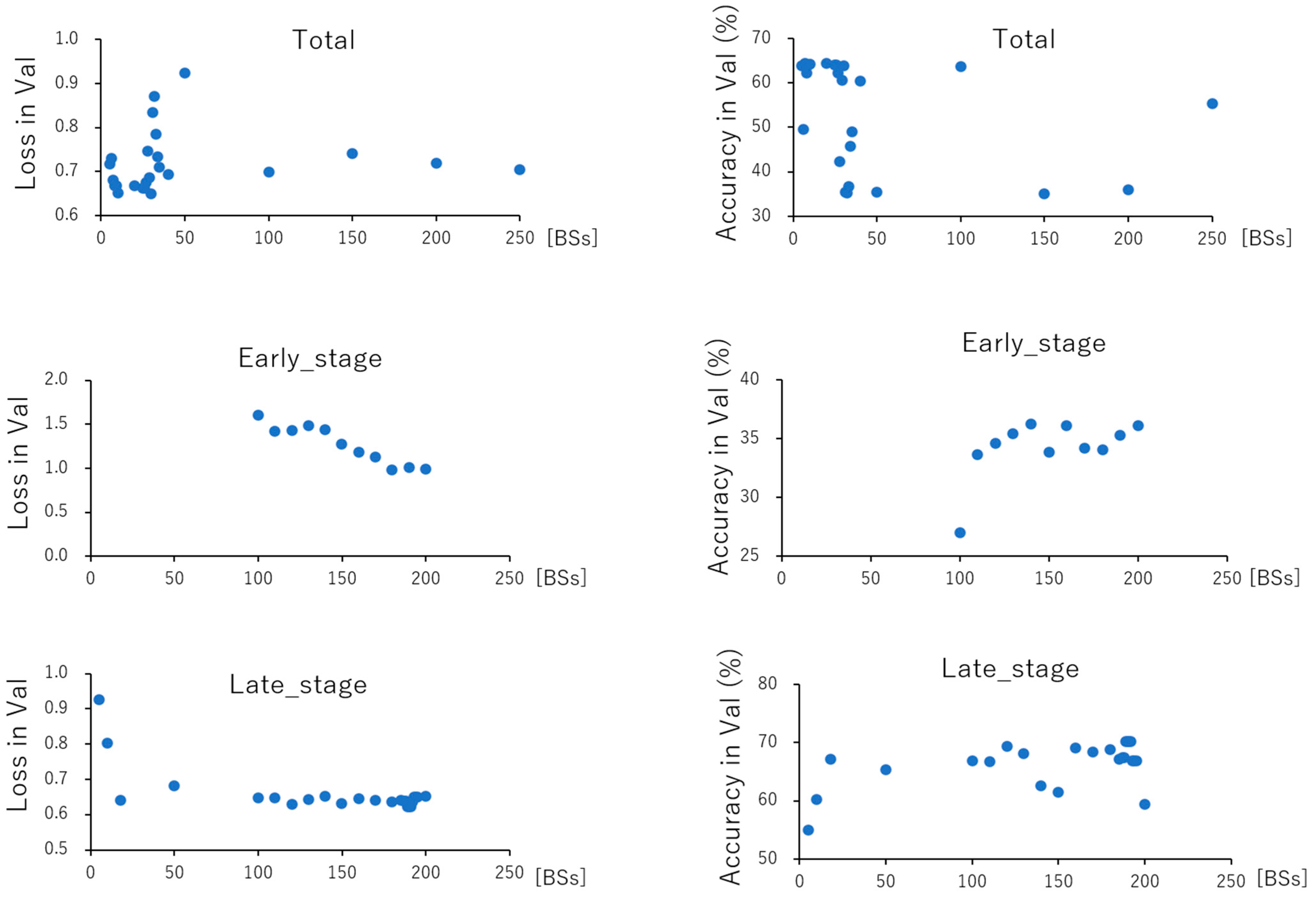
| Total ± SD | Early_Stage ± SD | Late_Stage ± SD | ||||
|---|---|---|---|---|---|---|
| mean loss (Val) | 0.718 | 0.068 | 1.268 | 0.220 | 0.660 | 0.067 |
| mean Acc (Val) | 53.7 | 11.8 | 35.3 | 3.1 | 66.3 | 3.9 |
| Total (BS) | Early_Stage (BS) | Late_Stage (BS) | ||||
|---|---|---|---|---|---|---|
| best loss (Val)/BS | 0.649 | 30 | 0.986 | 180 | 0.623 | 189 |
| best Acc (Val)/BS | 64.3 | 7 | 40.0 | 5 | 70.2 | 189, 190 |
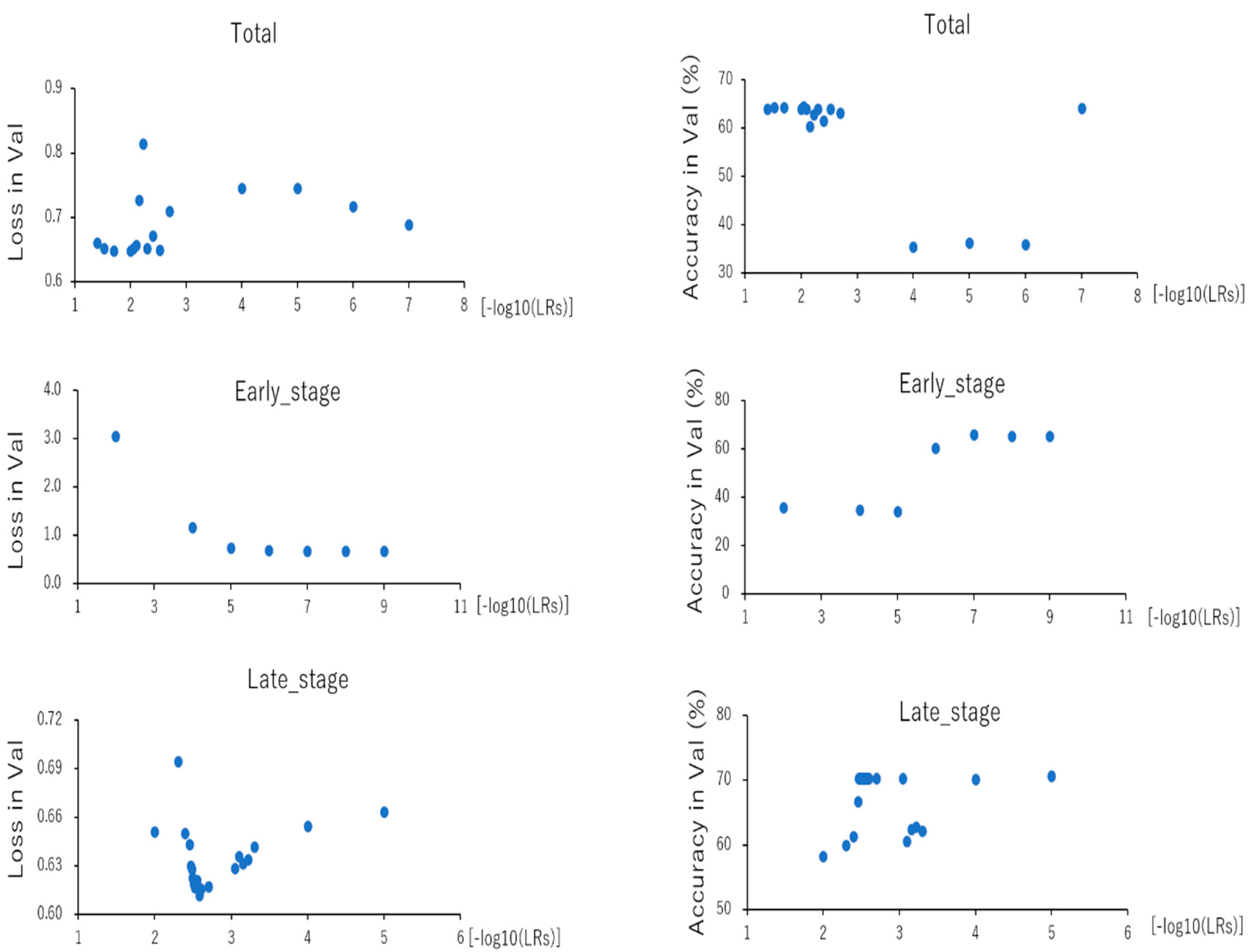
| Total ± SD | Early_Stage ± SD | Late_Stage ± SD | ||||
|---|---|---|---|---|---|---|
| mean loss (Val) | 0.690 | 0.049 | 1.099 | 0.879 | 0.634 | 0.020 |
| mean Acc (Val) | 58.2 | 11.2 | 51.7 | 15.8 | 67.2 | 4.4 |
| Total (LR) | Early_Stage (LR) | Late_Stage (LR) | ||||
|---|---|---|---|---|---|---|
| best loss (Val)/LR | 0.648 | 1.699 | 0.682 | 9.000 | 0.612 | 2.585 |
| best Acc (Val)/LR | 64.4 | 2.0 | 65.9 | 7.0 | 70.6 | 5.0 |
Publisher’s Note: MDPI stays neutral with regard to jurisdictional claims in published maps and institutional affiliations. |
© 2021 by the authors. Licensee MDPI, Basel, Switzerland. This article is an open access article distributed under the terms and conditions of the Creative Commons Attribution (CC BY) license (https://creativecommons.org/licenses/by/4.0/).
Share and Cite
Matsuzaka, Y.; Kusakawa, S.; Uesawa, Y.; Sato, Y.; Satoh, M. Deep Learning-Based In Vitro Detection Method for Cellular Impurities in Human Cell-Processed Therapeutic Products. Appl. Sci. 2021, 11, 9755. https://doi.org/10.3390/app11209755
Matsuzaka Y, Kusakawa S, Uesawa Y, Sato Y, Satoh M. Deep Learning-Based In Vitro Detection Method for Cellular Impurities in Human Cell-Processed Therapeutic Products. Applied Sciences. 2021; 11(20):9755. https://doi.org/10.3390/app11209755
Chicago/Turabian StyleMatsuzaka, Yasunari, Shinji Kusakawa, Yoshihiro Uesawa, Yoji Sato, and Mitsutoshi Satoh. 2021. "Deep Learning-Based In Vitro Detection Method for Cellular Impurities in Human Cell-Processed Therapeutic Products" Applied Sciences 11, no. 20: 9755. https://doi.org/10.3390/app11209755