
Processor-in-the-Loop Architecture Design and Experimental Validation for an Autonomous Racing Vehicle


Department of Mechanical and Aerospace Engineering, Politecnico di Torino, 10129 Torino, Italy
*
Author to whom correspondence should be addressed.
Appl. Sci. 2021, 11(16), 7225; https://doi.org/10.3390/app11167225
Submission received: 14 July 2021
/
Revised: 2 August 2021
/
Accepted: 3 August 2021
/
Published: 5 August 2021
(This article belongs to the Special Issue Frontiers in Mechatronics Systems for Automotive)
Abstract
:Self-driving vehicles have experienced an increase in research interest in the last decades. Nevertheless, fully autonomous vehicles are still far from being a common means of transport. This paper presents the design and experimental validation of a processor-in-the-loop (PIL) architecture for an autonomous sports car. The considered vehicle is an all-wheel drive full-electric single-seater prototype. The retained PIL architecture includes all the modules required for autonomous driving at system level: environment perception, trajectory planning, and control. Specifically, the perception pipeline exploits obstacle detection algorithms based on Artificial Intelligence (AI), and the trajectory planning is based on a modified Rapidly-exploring Random Tree (RRT) algorithm based on Dubins curves, while the vehicle is controlled via a Model Predictive Control (MPC) strategy. The considered PIL layout is implemented firstly using a low-cost card-sized computer for fast code verification purposes. Furthermore, the proposed PIL architecture is compared in terms of performance to an alternative PIL using high-performance real-time target computing machine. Both PIL architectures exploit User Datagram Protocol (UDP) protocol to properly communicate with a personal computer. The latter PIL architecture is validated in real-time using experimental data. Moreover, they are also validated with respect to the general autonomous pipeline that runs in parallel on the personal computer during numerical simulation.
1. Introduction
In recent years, huge research efforts have been dedicated to autonomous systems and self-driving ground vehicles, thus motivating the expectations of buying fully autonomous commercial cars within few decades, as reported in [1,2]. Autonomous driving is expected to drastically reduce car accidents and traffic, while robustly improving passenger comfort, as well as enhancing the capabilities of last-mile logistics and car sharing [3]. However, the development of autonomous systems is a complex multidisciplinary problem that must take into account social, economic, and technical issues for the next generation of vehicles [4,5,6]. Indeed, most of the current commercial cars can only experience Level 1 or 2 in the SAE J3106 Levels of Driving Automation scale. Therefore, there is still a wide research field to investigate, particularly related to the software developments and extensibility of further autonomous features.
To this end, racing competitions, such as Roborace [7], DARPA Grand Challenge [8], and Urban Challenge [9], have a pivotal role in the research and development of Level 4 and 5 automated vehicles. In fact, during the abovementioned competitions, self-driving cars race in a controlled and structured driving scenario, with little risk for human drivers and pedestrians, thus being a perfect environment for research of fully autonomous software pipelines and novel hardware solutions. In this framework, the present research work involves an all-wheel drive full-electric racing prototype participating at Formula Student Driverless (FSD) competitions.
A self-driving vehicle includes different modules devoted to specific functions, which are deeply interconnected in order to build the whole autonomous system. The main modules are environment perception, trajectory planning, and control, as reported in [10]. The perception module is responsible for the creation of an accurate representation of the environment around the vehicle at current status. Usually, the perception pipeline exploits the enhanced capability of artificial intelligence in combination with a plethora of sensors, such as multiple cameras, RADARs, and LiDARs, to guarantee sufficient redundancy and robustness [11,12]. Then, the trajectory planning module exploits the information computed from perception algorithms in order to define a proper and feasible trajectory that the vehicle has to follow. Different trajectory planning algorithms have been investigated in the recent literature [13,14], and efficient solutions for the retained racing prototype have been identified in the application of the Probabilistic Road Map (PRM) algorithm [15] and the RRT algorithms [16]. Finally, the control module is responsible for an accurate trajectory-following operation, while minimizing the tracking errors and maximizing the vehicle’s longitudinal speed, especially in the case of racing vehicles. To this end, a vast variety of control methods have been discussed in the literature for autonomous driving [13,17,18,19]. The retained PIL architecture embeds a MPC control strategy, as it is effective for the investigated application in prior research [16]. Moreover, the proposed trajectory planning method is based on a modified RRT algorithm based on Dubins curves, that exploits environment information from a vision-based perception pipeline.
PIL architecture is commonly used in different disciplines to test and validate the performance of a controlled system, as reported in [20,21,22]. The PIL approach allows verifying the actual control software running in a dedicated processor which controls a virtual model of the retained plant, as written in [21]. Therefore, PIL-based validation methods are used in different fields of study.
A PIL design and experimental validation is proposed in [23] for a MPC strategy devoted to Unmanned Aerial Vehicles (UAVs). The PIL architecture is also used for fast prototyping of power electronics circuits in [24]. Furthermore, the PIL layout is used to validate a hybrid fuzzy-RRT algorithm for indoor unmanned robots [25]. Although many applications involving autonomous ground vehicles exploit a hardware-in-the-loop (HIL) configuration, as in [26,27], the PIL approach is widely used for the validation of different control strategies and algorithms for automated driving. In detail, a software architecture for dynamic path planning of an autonomous racecar at the limits of handling is presented in [28] with a PIL configuration, and a focus on software implementation of the same application is illustrated in [29]. Moreover, a PIL architecture for prototyping purposes of urban motion planning and control is discussed in [30]. However, to the best of the authors’ knowledge, a study on the design and implementation of a PIL architecture for the experimental validation of trajectory planning and control algorithms for a full-electric autonomous racing prototype is still missing in the literature.
Considering the reported framework about PIL applications, the main contribution of this paper consists in the experimental validation of a PIL architecture for a fully autonomous racing prototype using a high-performance real-time target computing machine and a low-cost card-sized computer. Furthermore, the splitting of the PIL phase into two complementary steps leads to a genuine V-cycle process for the slender and rapid software development process for automotive industry application. From the software point-of-view a complete and customized pipeline for the perception, planning and control of an autonomous racing platform is proposed. Moreover, the motion planning problem is validated with real data acquisition on-board a racing vehicle. Specifically, the autonomous pipeline includes a trajectory planner based on a modified RRT algorithm and a control strategy based on MPC. Both the investigated PIL layouts communicate with a properly connected personal computer via UDP protocol. In the paper, different driving situations are shown for the retained racing vehicle. Furthermore, the proposed PIL architecture is validated with respect to a model-in-the-loop (MIL) architecture that runs only on the personal computer during numerical simulations, as discussed in [31]. In fact, MIL architecture includes testing the modeled plant on a dedicated simulation platform only. By contrast, PIL implementation allows to test the designed model when deployed on a target processor, in a closed-loop simulation layout. This step helps to identify if the investigated control algorithm can be deployed on the considered processor. In detail, the retained real-time computing machine is a Speedgoat Baseline platform, while the considered low-cost computer is a Raspberry Pi 4B board. The environment perception data come from a vision-based perception pipeline that exploits a stereocamera and LiDAR sensors which are properly mounted onto the vehicle. Specifically, the vehicle moves in a structured racing environment and the path is defined by multiple traffic cones of different colors, as defined in the FSD competitions.
The paper is structured as follows. Section 2 illustrates the general PIL architecture and the main modules of the retained autonomous system. Moreover, the hardware setup is discussed in detail and the considered computing platforms are described. Section 3 presents and discusses the obtained results on recorded experimental datasets for the MIL architecture and both the presented PIL layouts. Furthermore, a comparison with respect to the general autonomous pipeline that runs in parallel on the personal computer during simulation is presented. Finally, Section 4 concludes the paper.
2. Method
This section describes the design method of the proposed PIL architecture. First, starting from the perception pipeline installed on-board the racing vehicle, the retained software layout is defined. In detail, the proposed software layout assesses the motion planning task and control of the vehicle command inputs. Subsequently, the hardware setup and the connection specifications between the considered real-time target machines and the host personal computer are illustrated. Last, technical details of the considered computing platforms are highlighted with the objective of defining the PIL layout implications of both architectures.
2.1. Autonomous Vehicle Pipeline and Vehicle Setup
The considered vehicle is a fully electric all-wheel drive racing prototype with four on-wheel electric motor coupled with a highly efficient planetary transmission system concentrically mounted on each wheel hub. The vehicle has an integral carbon fiber chassis built with honeycomb panels, double wishbone push-rod suspensions, and a custom aerodynamic package. The vehicle can reach a maximum speed equal to 120 km/h with longitudinal acceleration peaks reaching up to 1.6 g. The main specifications of the racecar are listed in Table 1.
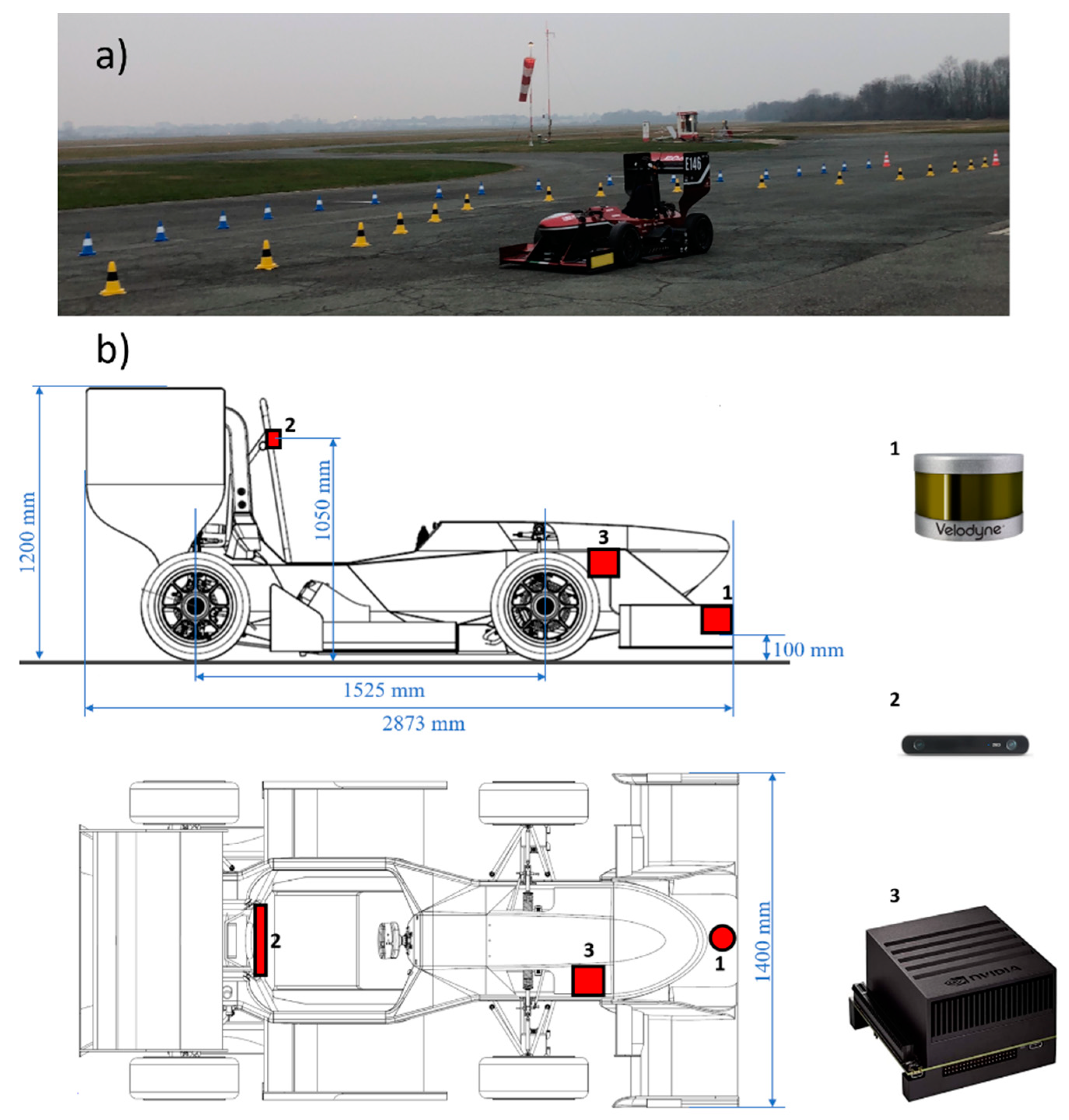
The vehicle senses the surrounding environment featuring a custom perception pipeline composed of a LiDAR-based sensor with an integrated high-performance Graphic Processing Unit (GPU) and a stereocamera. The former sensor is mounted in the middle of the front wing of the vehicle at a height of about 0.1 m from the ground. The latter instead is placed on the main roll hoop, above the driver’s seat. Both the sensors are interfaced with a properly designed Robotic Operating System (ROS) environment that can handle the measurements during vehicle’s motion and fuse them in order to provide real-time estimation about the position and type of surrounding obstacles. Specifically, the racing environment is structured with multiple traffic cones of different colors, as illustrated in Figure 1.
Information coming from the perception pipeline is then exploited for building a local map that enables the path planning method based on a modified version of RRT algorithm using Dubins curves.
Once the optimal path has been identified with respect to the goal position in each sensed local map, the investigated control strategy based on MPC assesses the vehicle dynamics control during motion. The vehicle is controlled via longitudinal acceleration and steering angle commands that are computed with respect to the planned path, while minimizing the tracking errors defined in terms of relative yaw angle and lateral deviation, as defined in [16,18,19].
The proposed PIL architecture is developed by deploying the planning and control methods into the retained real-time target platforms: a high-performance Speedgoat Baseline platform and low-cost Raspberry Pi 4B board. Both these target machines have been connected via UDP protocol to a host personal computer in which the retained vehicle model is accordingly defined. Figure 2 illustrates the retained autonomous pipeline and PIL architecture.
2.1.1. Environment Perception
As represented in Figure 1, the proposed environment perception pipeline is performed with a Velodyne VLP-16 LiDAR sensor, a Stereolabs ZED stereocamera, and a nVIDIA Jetson Xavier high-performance computing platform. In detail, the Velodyne VLP-16 LiDAR sensor is mounted onto the front wing of the vehicle at a fixed height equal to 0.1 m from the ground. The Stereolabs ZED stereocamera sensor is mounted at a height of 1.05 m from the ground and it is fixed to the vehicle’s rollbar, as represented in Figure 1. The NVIDIA Jetson Xavier high-performance computing platform is placed inside the vehicle’s monocoque, fixed to its right side. Moreover, a proper wiring system has been set up to correctly interface and supply the sensors to the computing platform.
The Velodyne VLP-16 LiDAR sensor provides a full 360-degree point cloud of the surrounding environment at a 10 Hz frequency to obtain an accurate real-time data reconstruction recorded by 16 light channels. It ranges up to 100 m with 30° vertical field-of-view (FOV) and an angular resolution up to 0.1° in the horizontal plane [32]. The LiDAR sensor is connected to the computing platform with embedded GPUs through an Ethernet connection. Specifically, the computing platform creates a ROS network, which allows to process the information streaming from the LIDAR-based sensor.
The Stereolabs ZED stereocamera is connected via 3.0 USB port to the computing platform. The considered stereocamera features stereo 2 K cameras with dual 4 MP RGB sensors. It is used as it is capable of accurately recording dense depth map information using triangulation from the geometric model of non-distorted rectified cameras up to 10 m in front of the vehicle [33]. To this end, left and right video frames are intrinsically synchronized and streamed so that several configuration parameters—resolution, brightness, contrast, and saturation—can be tuned properly [33]. Specifically, the camera is used in the high-definition 1080 mode (HD1080) at 30 Frame Per Second (FPS).
The NVIDIA Jetson AGX Xavier is an embedded Linux high-performance computing platform with embedded GPUs with 32 TOPS of peak computational power in less than 50 W of needed power. The retained high-performance computing platform enables intelligent vehicles with end-to-end autonomous capabilities as it is based on the most complex System-on-Chip (SoC) ever created up to 2018, thus enabling any complete artificial intelligence software stack [34].
The driving environment is properly structured with traffic cones according to the rules listed in [35] for the purpose of FSD competitions. In fact, each traffic cone has a height equal to 0.325 m and a square base, with a side length equal to 0.228 m. The cones of the right lane boundary are yellow with a black stripe, while the right lane boundary is built with blue cones with a white stripe. Bigger orange cones indicate the starting and the ending points of the track.
In this driving scenario, the LiDAR sensor records point clouds at a frequency equal to 10 Hz consisting of thousands of 3D point cloud during motion. Each point cloud contains the distance of each point in the 3D space along with the intensity of the reflected light in that point. Then, the raw point cloud is filtered by removing all the points out of the region-of-interest (ROI). Furthermore, a ground plane filtering segmentation algorithm is then applied to the raw point cloud in the considered ROI. This operation is performed in order to remove all the points belonging to the ground which can badly affect the proposed object detection method. Therefore, a clustering algorithm is applied to the filtered point cloud, then the distance to the detected obstacles is finally estimated.
In a similar way, the stereocamera-based perception algorithm is designed to detect cones and extract the color features from the detected obstacles, namely, blue, yellow, and orange cones. The distance with respect to the sensor is then computed by matching the detected bounding boxes representing the obstacles with the recorded depth map from the retained stereocamera. This algorithm is redundant to the LiDAR-based one. Nevertheless, it performs a peculiar task as it estimates not only the position of the detected obstacles, but also the color of the detected cones up to a 10 m distance from the sensor. In detail, the camera-based algorithm exploits a Single-Shot Detector (SSD) algorithm that is based on the Convolutional Neural Network (CNN) MobileNet v1.
As a result of the implemented perception algorithms, a local map containing the information about the obstacles in front of the vehicle is created at a 10 Hz frequency, that enables further trajectory planning and control methods. Specifically, the information about obstacles includes position about the obstacles in the x-y plane and a color tag.
2.1.2. Path Planning
The trajectory planning algorithm generates the feasible poses that the vehicle has to follow acting on the acceleration/deceleration and steering commands which are computed by the designed MPC controller. Thus, the objective of the designed path planning algorithm is to find a collision-free motion between the start and goal positions of the vehicle in a structured environment. The environment where the vehicle moves is defined by the perception stage.
The vehicle explores the environment using a real-time local trajectory planner, based on a modified RRT algorithm for non-holonomic car-like mobile robots, using Dubins curves. The algorithm takes into account kinematic and dynamic constraints of the vehicle, as defined in [36], in addition to the pure geometric problem of obstacle avoidance, and allows to search non-convex high-dimensional spaces by randomly building a space-filling tree [37]. The RRT algorithm is based on the incremental construction of a search tree that attempts to rapidly and uniformly explore obstacle-free segment in the configuration space. Once a search tree is successfully created, a simple search operation among the branches of the tree can result in collision-free path between any two points in vehicle environment. Due to differential constraints of non-holonomic car-like mobile robots, the set of potential configurations that a vehicle can reach from a certain state is reduced and Dubins curves are selected for building the branches in the search tree instead of the straight lines, as it is discussed in [23].
The initial position of the vehicle is always retained in the origin of the frame at the considered sampling time. The detected cones on the two-dimensional map are used to discretize the space within which the vehicle is moving through the Delaunay Triangulation algorithm [38], i.e., an iterative search technique based on the assumption that one and only one circumference passes through three non-aligned points. Considering the obstacles detected by the perception pipeline, a circumference passing by them is computed for each random triplet of points. As a result of the iterative process that is repeated until all possible combinations of points are investigated during Delaunay Triangulation, the final goal is selected among the potential goal points, considering the farthest point with respect to the vehicle initial position. Afterwards, the search tree is built and updated each time new vehicle state is available. The minimum turning radius is set on the basis of the vehicle steering specification, as the maximum front steering angle that is equal to during turns, and it is equal to when the vehicle is accelerating. The implemented RRT algorithm exploits Dubins curves to connect two consecutive vertices, as the shortest path is expressed as a combination of no more than three primitive curves. In this research work, three different types of primitive curves are considered. The primitive drives the car straight ahead, while the and primitives turn as sharply as possible to the left and right, respectively. As discussed in [39], ten combinations of primitive curves are possible, but only six primitives can be optimal, and they are properly named Dubins curves. The possible combinations are listed below:
where and denote the total amount of accumulated rotation and , , is the distance travelled along the straight segment, . A robust theoretical background about Dubins segments can be found in [39]. Finally, the cumulative length of the path is given by the sum of the length of its constituent segments. In the proposed algorithm, the shortest path is chosen, i.e., the one with the lowest . Furthermore, the planned path must be feasible and collision-free, thus the paths which hit obstacles are discarded. The investigated trajectory planning method is thus able to compute a feasible trajectory that is consistent with the performance of an autonomous steering actuator, as discussed in [40]. Afterwards, the speed profile can be associated to the selected path based on the limitations imposed by the vehicle dynamics. Therefore, during turns, the speed is limited by the maximum lateral acceleration that is equal to 2 . In the same way, the reference speed profile is constrained by the longitudinal speed and acceleration on a straight path. The upper bound of the longitudinal speed is 30 , according to the vehicle’s maximum speed. The vehicle longitudinal acceleration peaks can reach up to 1.6 . Moreover, as the vehicle should not go in reverse, the lower bound is imposed equal to 0 . Under these assumptions, the minimum value of the velocity is computed as follows:
where is the curvature of the computed path. Given the coordinates of each sample of the path, is geometrically computed as follows:
2.1.3. Vehicle Modeling
This section describes the released vehicle and tire models that are used for trajectory planning algorithm test and validation purposes. Several mathematical models have been investigated in the recent literature with different levels of complexity and accuracy based on the research context [41]. In this paper, the vehicle is modeled using the 3-DOF rigid vehicle model (single track) for both lateral and longitudinal dynamics as depicted in Figure 3.
The equations of motion are written in terms of errors with respect to the reference poses generated by the Local Path Planner to properly define the controller variables. To this extent, the kinematic motion of the vehicle, at velocity , can be described with the cross-track error of the front axle guiding wheels, and the angle of those wheels with respect to the nearest segment of the trajectory to be tracked , as reported in Figure 4.
In case of forward driving motion and steering system acting only on vehicle front guiding wheels, the derivative of the cross-track error and relative yaw angle can be defined as follows:
where is the lateral velcity in the vehicle-fixed reference frame, is the heading angle of the vehicle with respect to the closest trajectory segment, and is the angle of the front wheels with respect to the vehicle. The steering is mechanically limited to and . The derivative of the heading angle is
where and are the distance from the center of gravity (CoG) to the front and rear wheels, respectively.
The vehicle model takes in consideration also the nonlinear dynamic motion contribution coming from the effect of the tire slip and the steering servomotor that actuates the steering system mechanism. The front and rear tires are modeled such that each provides a force and , perpendicular to the rolling direction of the tire, and proportional to the side slip angle . Assuming negligible vehicle track, the lateral forces at the front and rear wheels are entirely due to the contribution coming from the tires:
where and refers to the lateral stiffness of the front and rear tires, respectively. Then, the front and rear tire side slip angles can be defined as
with vehicle-fixed longitudinal and lateral velocities and . In the end, the equations of motion can be written as
where and are the components of the force provided by the front and rear tires in their direction of rolling.
Thus, the equation of motion (11)–(13) are rewritten in terms of the cross-track error and relative yaw angle . The state space equation of the obtained model state space model is defined in Equation (14).
In addition, the state space model presented in Equation (14) is also used as reference model for the control strategy presented in the following section.
2.1.4. Control
The vehicle control computes the front wheel steering angle and throttle/brake command to track the reference trajectory. Similar to the work presented in [18,42], a MPC strategy is applied to compute the acceleration/deceleration and front wheel steering angle commands for the racing vehicle. Two different MPC controllers are used to achieve the lateral and longitudinal vehicle dynamics, respectively.
The MPC dealing with the lateral vehicle dynamics applies an internal vehicle model defined by the state space representation in Equation (14) to predict the future behavior of the controlled system on the prediction horizon . The MPC takes as input the crosstrack error and the relative yaw angle defined in (4) and (5).
Then, it solves an open-loop optimal control problem to determine the optimal commands, that is defined as where is the control horizon. Therefore, only the first input of the optimal control sequence is applied to the system, and the prediction horizon is shifted one step forward to repeat the prediction and optimization procedure on the new available vehicle states. The optimization problem to be solved at each time step is
subject to
where is the control command, is the predicted value of the -th output plant at the -th prediction horizon step, and is the reference value for the -th output plant at the -th prediction horizon step. The weighted norms of vector and are equal to
and are the design matrices chosen according to the desired performance trade off.
The optimization problem is formulated to minimize the sum of the weighted norms of the control input variables and the error between the predicted output vector and the reference output vector which are computed as
while the operational constraints to which the optimization problem is subject are
2.2. Hardware Implementation and PIL Architecture
Novel vehicle functions verification and features validation hold increasingly critical importance in the development of on-board vehicle software–hardware platforms. Generally, software implementation of ADAS or Autonomous Driving functions require a development process aimed at improving the overall quality of the software, increasing the development efficiency, and eliminating systematic software bugs. To this extent, the V-cycle process represents the adequate software development process widely used in automotive industry field applications, as represented in Figure 5. The typical V-cycle process insists on a top-down approach for what concerns the designing phase and a bottom-up approach for the validation one. Performing the descending phase of the cycle, the process ensures that the high-level system requirements are respected. On the contrary, the ascending stages avoids costly system-level testing before the functional components have been demonstrated [43]. This section will focus on the descending stages of the V-cycle development process, treating up the embedded software generation for the retained real-time target machines.
Algorithms are implemented in the MATLAB/Simulink environment which deploys a model-based design approach that automatically generates embedded software for the target machine. Moreover, the retained MATLAB/Simulink environment is used to create different test case scenarios and verify results for different testing simulation procedures such as model-in-the-loop (MIL) and processor-in-the-loop (PIL).
In this work, MIL contains all the subsystems (perception, motion planning, and control, and vehicle model) needed to perform the simulation. Conversely, the retained PIL setup splits these components into two groups: a first set running on the target computer with a compiled application, containing the motion planning and control, and another set, i.e., the vehicle model only, running on the host PC. The command input for the vehicle model plant on the host PC, i.e., the steering angle at the wheels and the acceleration command, are sent via UDP, along with the fed-back information of the vehicle state running on the real-time target machine. UDP is a packet-based protocol that uses an Ethernet board as physical layer. This protocol is advantageous for real-time application because has smaller delay than TCP connection as it does not retransmit lost packets. To this extent, UDP Send and Receive blocks are set in the MATLAB/Simulink environment to interface with the motion planner and controller (target side), as well as the vehicle plant model (host side). Furthermore, simulation pacing option is set to obtain near-real-time simulation also on model running on development computer, thus forcing the synchronization between the plant model running on the development computer and the controller flashed onto the target device. The setup of the PIL test using the Speedgoat Real Time target machine is shown in Figure 6, while the PIL test setup exploiting the functionality of Raspberry Pi 4B board is represented in Figure 7.
In the preliminary phase of the performed software implementation, it was decided to deploy the embedded software on a low-cost platform, i.e., the Raspberry Pi 4B board with hardware specification shown in Table 2. Raspberry Pi is a small-sized, general-purpose computing device that is capable of running any ARM-compatible operating system. By having an open-source environment, Linux facilitates the application of the Raspberry Pi in the development of embedded control devices. In addition, its integration with MATLAB/Simulink environment facilitates the application building and deployment onto the aforementioned platform. However, the Linux operating system is not designed to work with real-time applications and predictive processing [44] unless the RT-Preempt patch is installed on the Raspberry Pi, thus creating a para-virtualized design which allows to use a micro-kernel running in parallel to the standard Linux kernel [45]. To this extent, at this introductory stage, the objective of the work was to evaluate the feasibility of implementing the Motion Planning and Motion Control custom algorithms using low-cost equipment without considering real time constraints, but effectively assessing the overall algorithm efficiency, comparing I/O signals in MIL/PIL configurations. On average, the processor worked for 50% of its total computing power with a maximum RAM memory allocation of about 10%. In accordance with the signals’ setup that the aforementioned platform exchanges with the host PC, the numeric data type of each signal has been chosen in order to give a sufficient precision for each computational tasks required by the application flashed on the board.
Subsequently, the PIL architecture has been configured for the Speedgoat Baseline real-time target machine with hardware specification shown in Table 2. Thus, the model containing the motion planning and motion control running on the Speedgoat machine was validated considering real-time constraints. Motion planning takes a relatively large computational time to generate the search tree expansion and select the path with the shortest distance to the goal position. On the other hand, the motion control must be executed in fast time loops to obtain state feedback, more precise actuator control and trajectory tracking. To this extent, in our implementation, motion planning component is configured to run every 50 , while motion controller runs at higher sample rate, i.e., 10 , the same sample rate defined for MIL architecture. On average the Motion Planner is executed with a Target Execution Time (TET) of 0.043 while the Motion Control every 0.008 .
3. Results
Three test cases for MIL and PIL architectures are illustrated during different maneuvers. The validation dataset has been recorded during a real acquisition stage performed on-board the racing vehicle instrumented with LiDAR and stereocamera sensors and a high-performance computing platform with embedded GPU. The perception pipeline acquires the structured environment with a frequency of 10 Hz. The whole validation dataset includes several maneuvers performed by the vehicle in the racing environment that was properly structured with traffic cones according to the rules listed in [35].
3.1. Driving Scenarios and Environment Perception
In Figure 8, Figure 9 and Figure 10, the planned trajectory is represented by a red solid line, while the search tree is represented by a dashed black line. The initial vehicle position is labeled with a red asterisk and the goal position is indicated by a red triangle. The detected cones are represented with black dots. In the first maneuver, the self-driving vehicle travels a straight road portion with a reference longitudinal speed of 22.2 , while in the second and third one the autonomous racing vehicle travels a left/right constant radius turn of 50 with a reference longitudinal speed set at 13.8 .
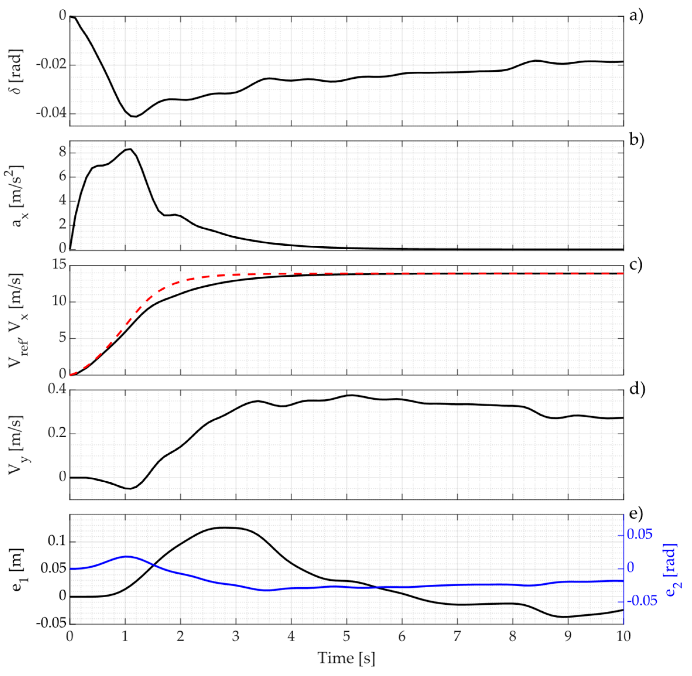
The vehicle main states are reported in Figure 11, Figure 12 and Figure 13 for the maneuvers performed in Figure 8, Figure 9 and Figure 10, respectively. In Figure 11, Figure 12 and Figure 13, the front wheel steering angle and the longitudinal acceleration commands are shown in subfigures a and b. Subfigure c illustrates the reference longitudinal speed (red dashed line) with respect to the actual vehicle speed (black solid line). The lateral velocity is shown in subfigure d, while the cross-track error (black line) and the angle (blue line) are shown in subfigure e for each maneuver.
Figure 8 represents a frame sensed on a straight road portion. As shown in Figure 11, the vehicle follows accurately the speed profile. The front wheel steering angle remains steady at 0 (Figure 11a). The longitudinal acceleration has a maximum peak value of 9.5 (Figure 11b), while the longitudinal velocity rapidly reaches its steady-state value of 22.2 (Figure 11c). Lateral velocity (Figure 11d) and the cross-track error and the angle remain null for all the simulation time (Figure 11e).
Figure 9 represents the frame sensed during a left turn maneuver. The final goal is located almost on the centerline of the track defined by the cones. As shown in Figure 12, the vehicle follows accurately the speed profile (Figure 12c) and the longitudinal acceleration reaches about 8 (Figure 12b). The front wheel steering angle increases up to 0.2 and then decreases till stabilizing in steady-state condition at 0.02 (Figure 12a). The cross-track error and the relative yaw angle oscillate in the first phase of the maneuver and then stabilize to null values (Figure 12e).
Figure 10 represents the frame sensed during a right turn maneuver. The final goal is located almost on the midpoint of the line generated by the two rows of cones, approximately 15 far from the vehicle local position. As shown in Figure 13, the vehicle follows accurately the speed profile and the longitudinal acceleration reaches up to 8 while the longitudinal velocity increases from 0 up to 13.8 , as illustrated in Figure 11b,c, respectively. The front wheels steering angle decreases up to −0.04 and then remains almost constant at −0.02 (Figure 13a). The cross-track error and the relative yaw angle are always within ± 0.1 (Figure 13e).
In all the considered maneuvers, the vehicle follows the planned trajectory and respects the feasibility constraints imposed by the actuators, in terms of maximum front wheel steering angle, and vehicle dynamics, while maximizing its longitudinal speed.
3.2. Processor-in-the-Loop and Simulations Comparison
In this section, a comparative analysis of the obtained results using PIL architectures with respect to the MIL one is discussed. Vehicle main states extracted from the PIL architecture with the Raspberry Pi 4B board and Speedgoat real-time target machine are compared and validated employing the same real acquisition dataset. This dataset includes the maneuvers illustrated in the previous section.
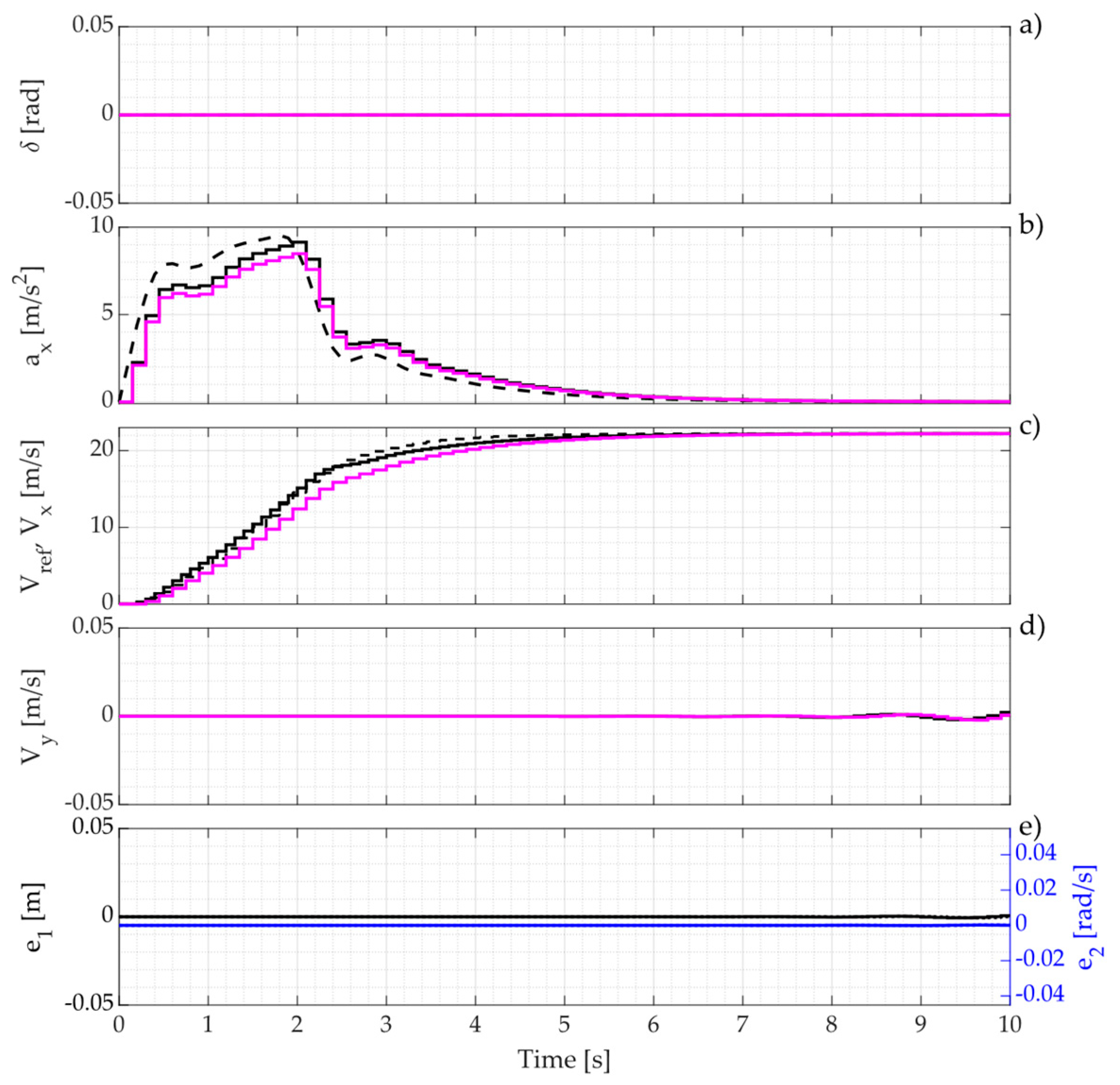
The vehicle main states are reported in Figure 14, Figure 15 and Figure 16 for the maneuvers performed in Figure 8, Figure 9 and Figure 10, respectively. In Figure 14, Figure 15 and Figure 16, the front wheel steering angle extracted from PIL architecture with the Raspberry Pi 4B board (magenta, solid) and Speedgoat real-time target machine (black, solid) is compared with respect to the MIL configuration output (black, dashed) in subfigure a. The longitudinal acceleration command from MIL architecture (black, dashed) is shown in subfigure b along with the acceleration command resulting from both PIL architectures, Raspberry Pi 4B board (magenta, solid) and Speedgoat real-time target machine (black, solid), respectively. Subfigure c illustrates the reference longitudinal speed (black, dashed) with respect to the actual vehicle speed in PIL configurations . The lateral velocity is shown in subfigure d, while the crosstrack error (black, solid for Speedgoat real-tim target machine and black, dotted for Raspberry Pi 4B board) and the angle (blue, solid for Speedgoat real-time target machine and blue, dotted for Raspberry Pi 4B board) are shown in subfigure e, for each maneuver comparing MIL/PIL architectures.
Considering the comparison between MIL and PIL configurations, the vehicle states and the control variables are comparable, thus proving the consistency of the proposed PIL architecture.
In Table 3, Root Mean Square Error (RMSE) and the Mean Absolute Error (MAE) for the controlled variables calculated in both PIL configurations, and , are reported. The performances of both PIL layout are also reported in terms of driving Scenarios performed by the retained self-driving vehicle. The RMSE and the MAE are defined as
where represents the difference between the observed controlled variable in PIL configuration and the reference one obtained in MIL configuration, while represents the number of observations.
4. Conclusions
In this work, an experimental software development process for rapid prototyping of AD features in the automotive field is presented. Exploiting the functionalities of two different embedded systems—Raspberry Pi 4B board and Speedgoat Baseline real-time target machine, a trajectory planning method for an autonomous racing vehicle was implemented, developing two PIL complementary architectures. The investigated trajectory planning method proposed a custom realization of the RRT algorithm with Dubins curves able to compute a feasible trajectory, considering a 3-DOF linear bicycle vehicle model. The autonomous racing vehicle dynamics is controlled with a MPC that computes the front wheel steering angle and longitudinal acceleration commands in feedback loop with respect to the vehicle plant.
The method was first tested in MIL configuration in a properly structured driving environment, that features multiple traffic cones representing non-crossable obstacles. The consistency of the planned trajectory was evaluated during different maneuvers, and it was also evaluated in terms of feasibility of the command signals with respect to the steering and acceleration actuators used in the retained vehicle.
Subsequently, the PIL architecture is defined by splitting the components of the model in two groups: a first set running on the target computer with a compiled application, containing the motion planning and control, and another set, i.e., the vehicle model only, running on the host PC. Signals exchanged between target hardware and host PC are sent via UDP protocol. The first PIL architecture was built using the Raspberry Pi 4B board with the objective of testing the software efficiency and signals calculation precision. Afterwards, the PIL architecture was switched to the Speedgoat Baseline real-time target machine in order to consider the real-time constraints and control average TET. Subsequently, a quantitative analysis has been performed between MIL and PIL architectures to further prove the consistency of the two investigated layouts.
The PIL procedures demonstrate that the proposed architectures provide relevant results within the framework of V-cycle development process, ensuring that new functionalities of self-driving vehicle can be rapidly deployed, tested, and validated on generic-purpose platforms. This approach considerably decreases the time to proceed towards the hardware-in-the-loop (HIL) stage. A further extensive experimental validation phase is needed before generalization of the approach to any automotive systems.
Author Contributions
Conceptualization, E.T., S.L., S.F. and A.B.; methodology, E.T., S.L. and S.F.; software, E.T., S.L. and S.F.; validation, E.T., S.L. and S.F.; investigation, E.T., S.L. and S.F.; writing—original draft preparation, E.T., S.L. and S.F.; writing—review and editing, E.T., S.L. and S.F.; visualization, E.T., S.L. and S.F.; supervision, A.B. and N.A.; project administration, A.B. and N.A. All authors have read and agreed to the published version of the manuscript.
Funding
This research received no external funding.
Institutional Review Board Statement
Not available.
Informed Consent Statement
Not available.
Data Availability Statement
Data available on request due to restrictions.
Acknowledgments
This work was developed in the framework of the activities of the Interdepartmental Center for Automotive Research and Sustainable mobility (CARS) at Politecnico di Torino (www.cars.polito.it, accessed on 3 August 2021).
Conflicts of Interest
The authors declare no conflict of interest.
References
- Chan, C.Y. Advancements, prospects, and impacts of automated driving systems. Int. J. Transp. Sci. Technol. 2017, 6, 208–216. [Google Scholar] [CrossRef]
- Silberg, G.; Manassa, M.; Everhart, K.; Subramanian, D.; Corley, M.; Fraser, H.; Sinha, V. Self-driving cars: Are we ready? Kpmg Llp 2013, 1–36. [Google Scholar]
- Litman, T. Autonomous Vehicle Implementation Predictions; Victoria Transport Policy Institute: Victoria, CB, Canada, 2017; p. 28. [Google Scholar]
- Ryan, M. The future of transportation: Ethical, legal, social and economic impacts of self-driving vehicles in the year 2025. Sci. Eng. Ethics 2020, 26, 1185–1208. [Google Scholar] [CrossRef] [PubMed] [Green Version]
- Raposo, M.A.; Grosso, M.; Mourtzouchou, A.; Krause, J.; Duboz, A.; Ciuffo, B. Economic implications of a connected and automated mobility in Europe. Res. Transp. Econ. 2021, 101072. [Google Scholar] [CrossRef]
- Bagloee, S.A.; Tavana, M.; Asadi, M.; Oliver, T. Autonomous vehicles: Challenges, opportunities, and future implications for transportation policies. J. Mod. Transp. 2016, 24, 284–303. [Google Scholar] [CrossRef] [Green Version]
- Rieber, J.M.; Wehlan, H.; Allgower, F. The ROBORACE contest. IEEE Control Syst. Mag. 2004, 24, 57–60. [Google Scholar]
- Thrun, S.; Montemerlo, M.; Dahlkamp, H.; Stavens, D.; Aron, A.; Diebel, J.; Fong, P.; Gale, J.; Halpenny, M.; Hoffmann, G.; et al. Stanley: The robot that won the DARPA Grand Challenge. J. Field Robot. 2006, 23, 661–692. [Google Scholar] [CrossRef]
- Buehler, M.; Iagnemma, K.; Singh, S. (Eds.) The DARPA Urban Challenge: Autonomous Vehicles in City Traffic; Springer: Berlin/Heidelberg, Germany, 2009; Volume 56. [Google Scholar]
- Pendleton, S.D.; Andersen, H.; Du, X.; Shen, X.; Meghjani, M.; Eng, Y.H.; Rus, D.; Ang, M.H. Perception, planning, control, and coordination for autonomous vehicles. Machines 2017, 5, 6. [Google Scholar] [CrossRef]
- Kocić, J.; Jovičić, N.; Drndarević, V. Sensors and sensor fusion in autonomous vehicles. In Proceedings of the 26th Telecommunications Forum (TELFOR), Belgrade, Serbia, 20–21 November 2018; pp. 420–425. [Google Scholar]
- Feraco, S.; Bonfitto, A.; Amati, N.; Tonoli, A. A LIDAR-Based Clustering Technique for Obstacles and Lane Boundaries Detection in Assisted and Autonomous Driving. In Proceedings of the ASME 2020 International Design Engineering Technical Conferences and Computers and Information in Engineering Conference, St. Louis, MO, USA, 16–19 August 2020. [Google Scholar]
- Katrakazas, C.; Quddus, M.; Chen, W.H.; Deka, L. Real-time motion planning methods for autonomous on-road driving: State-of-the-art and future research directions. Transp. Res. Part C Emerg. Technol. 2015, 60, 416–442. [Google Scholar] [CrossRef]
- Schwarting, W.; Alonso-Mora, J.; Rus, D. Planning and decision-making for autonomous vehicles. Annu. Rev. Control Robot. Auton. Syst. 2018, 1, 187–210. [Google Scholar] [CrossRef]
- Feraco, S.; Bonfitto, A.; Khan, I.; Amati, N.; Tonoli, A. Optimal Trajectory Generation Using an Improved Probabilistic Road Map Algorithm for Autonomous Driving. In Proceedings of the International Design Engineering Technical Conferences and Computers and Information in Engineering Conference, Online Conference, 17–19 August 2020; Volume 83938, p. V004T04A006. [Google Scholar]
- Feraco, S.; Luciani, S.; Bonfitto, A.; Amati, N.; Tonoli, A. A local trajectory planning and control method for autonomous vehicles based on the RRT algorithm. In Proceedings of the 2020 AEIT International Conference of Electrical and Electronic Technologies for Automotive (AEIT AUTOMOTIVE), Online Conference, 18–20 November 2020; pp. 1–6. [Google Scholar]
- Yurtsever, E.; Lambert, J.; Carballo, A.; Takeda, K. A survey of autonomous driving: Common practices and emerging technologies. IEEE Access 2020, 8, 58443–58469. [Google Scholar] [CrossRef]
- Khan, I.; Feraco, S.; Bonfitto, A.; Amati, N. A Model Predictive Control Strategy for Lateral and Longitudinal Dynamics in Autonomous Driving. In Proceedings of the ASME 2020 International Design Engineering Technical Conferences and Computers and Information in Engineering Conference, St. Louis, MO, USA, 16–19 August 2020. [Google Scholar]
- Feraco, S.; Bonfitto, A.; Amati, N.; Tonoli, A. Combined lane keeping and longitudinal speed control for autonomous driving. In Proceedings of the ASME 2019 International Design Engineering Technical Conferences and Computers and Information in Engineering Conference, Anaheim, CA, USA, 18–21 August 2019. [Google Scholar]
- Mina, J.; Flores, Z.; López, E.; Pérez, A.; Calleja, J.H. Processor-in-the-loop and hardware-in-the-loop simulation of electric systems based in FPGA. In Proceedings of the 13th International Conference on Power Electronics (CIEP), Mexico Guanajuato, Mexico, 20–23 June 2016; pp. 172–177. [Google Scholar]
- Hu, M.; Zeng, G.; Yao, H.; Tang, Y. Processor-in-the-loop demonstration of coordination control algorithms for distributed spacecraft. In Proceedings of the 2010 IEEE International Conference on Information and Automation, Harbin, China, 20–23 June 2010; pp. 1008–1011. [Google Scholar]
- Francis, G.; Burgos, R.; Rodriguez, P.; Wang, F.; Boroyevich, D.; Liu, R.; Monti, A. Virtual prototyping of universal control architecture systems by means of processor in the loop technology. In Proceedings of the APEC 07-Twenty-Second Annual IEEE Applied Power Electronics Conference and Exposition, Anaheim, CA, USA, 25 February–1 March 2007; pp. 21–27. [Google Scholar]
- Mammarella, M.; Capello, E.; Park, H.; Guglieri, G.; Romano, M. Tube-based robust model predictive control for spacecraft proximity operations in the presence of persistent disturbance. Aerosp. Sci. Technol. 2018, 77, 585–594. [Google Scholar] [CrossRef]
- Vardhan, H.; Akin, B.; Jin, H. A low-cost, high-fidelity processor-in-the loop platform: For rapid prototyping of power electronics circuits and motor drives. IEEE Power Electron. Mag. 2016, 3, 18–28. [Google Scholar] [CrossRef]
- Taheri, E.; Ferdowsi, M.H.; Danesh, M. Fuzzy greedy RRT path planning algorithm in a complex configuration space. Int. J. Control Autom. Syst. 2018, 16, 3026–3035. [Google Scholar] [CrossRef]
- Deng, W.; Lee, Y.H.; Zhao, A. Hardware-in-the-loop simulation for autonomous driving. In Proceedings of the 2008 34th Annual Conference of IEEE Industrial Electronics, Orlando, FL, USA, 10–13 November 2008; pp. 1742–1747. [Google Scholar]
- Brogle, C.; Zhang, C.; Lim, K.L.; Bräunl, T. Hardware-in-the-loop autonomous driving simulation without real-time constraints. IEEE Trans. Intell. Veh. 2019, 4, 375–384. [Google Scholar] [CrossRef]
- Betz, J.; Wischnewski, A.; Heilmeier, A.; Nobis, F.; Hermansdorfer, L.; Stahl, T.; Herrmann, T.; Lienkamp, M. A software architecture for the dynamic path planning of an autonomous racecar at the limits of handling. In Proceedings of the 2019 IEEE International Conference on Connected Vehicles and Expo (ICCVE), Graz, Austria, 4–8 November 2019; pp. 1–8. [Google Scholar]
- Betz, J.; Wischnewski, A.; Heilmeier, A.; Nobis, F.; Stahl, T.; Hermansdorfer, L.; Lienkamp, M. A software architecture for an autonomous racecar. In Proceedings of the 2019 IEEE 89th Vehicular Technology Conference (VTC2019-Spring), Kuala Lumpur, Malaysia, 28 April–1 May 2019; pp. 1–6. [Google Scholar]
- Sun, Y.; Goila, A.; Demir, D.; Tapli, T. Urban Pilot Motion Planning and Control Deployment Via Real-Time Multi-Core Multi-Thread Prototyping (No. 2020-01-0125). In SAE Technical Paper; 2020. Available online: https://www.sae.org/publications/technical-papers/content/2020-01-0125/ (accessed on 14 July 2021).
- Srinivas, N.; Panditi, N.; Schmidt, S.; Garrelfs, R. MIL/SIL/PIL Approach A new paradigm in Model Based Development. J. Syst. Softw. 2014. Available online: https://www.mathworks.com/content/dam/mathworks/mathworks-dot-com/solutions/automotive/files/in-expo-2014/mil-sil-pil-a-new-paradigm-in-model-based-development.pdf (accessed on 14 July 2021).
- Glennie, C.L.; Kusari, A.; Facchin, A. Calibration and Stability Analysis of the VLP-16 Laser Scanner. ISPRS Annals of Photogrammetry. Remote Sens. Spat. Inf. Sci. 2016, 9. Available online: https://www.int-arch-photogramm-remote-sens-spatial-inf-sci.net/XL-3-W4/55/2016/isprs-archives-XL-3-W4-55-2016.pdf (accessed on 14 July 2021).
- Ortiz, L.E.; Cabrera, E.V.; Gonçalves, L.M. Depth data error modeling of the ZED 3D vision sensor from stereolabs. ELCVIA Electron. Lett. Comput. Vis. Image Anal. 2018, 17, 0001-15. [Google Scholar] [CrossRef]
- Ditty, M.; Karandikar, A.; Reed, D. Nvidia’s xavier SoC. In Proceedings of the Hot Chips: A Symposium on High Performance Chips, Cupertino, CA, USA, 19–21 August 2018. [Google Scholar]
- Formula Student Germany. FSG Competition Handbook 2019; 2019. Available online: https://www.formulastudent.de/fileadmin/user_upload/all/2019/rules/FSG19_Competition_Handbook_v1.0.pdf (accessed on 14 July 2021).
- Živojević, D.; Velagić, J. Path planning for mobile robot using Dubins-curve based RRT algorithm with differential constraints. In Proceedings of the 2019 International Symposium ELMAR, Zadar, Croatia, 23–25 September 2019; pp. 139–142. [Google Scholar]
- LaValle, S.M. Rapidly-Exploring Random Trees: A New Tool for Path Planning; 1998. Available online: http://lavalle.pl/papers/Lav98c.pdf (accessed on 14 July 2021).
- Delaunay, B. Sur la sphere vide, Otdelenie Matematicheskii i Estestvennyka Nauk 7. Izv. Akad. Nauk SSSR 1934, 1–2, 793–800. [Google Scholar]
- Dubins, L.E. On curves of minimal length with a constraint on average curvature, and with prescribed initial and terminal positions and tangents. Am. J. Math. 1957, 79, 497–516. [Google Scholar] [CrossRef]
- Manca, R.; Circosta, S.; Khan, I.; Feraco, S.; Luciani, S.; Amati, N.; Bonfitto, A.; Galluzzi, R. Performance Assessment of an Electric Power Steering System for Driverless Formula Student Vehicles. In Actuators; Multidisciplinary Digital Publishing Institute: 2021; Volume 10, p. 165. Available online: https://www.mdpi.com/2076-0825/10/7/165 (accessed on 14 July 2021).
- Li, L.; Wang, F.; Zhou, Q. Integrated longitudinal and lateral tire/road friction modeling and monitoring for vehicle motion control. IEEE Trans. Intell. Transp. Syst. 2016, 7, 1–19. [Google Scholar] [CrossRef]
- Luciani, S.; Bonfitto, A.; Amati, N.; Tonoli, A. Model predictive control for comfort optimization in assisted and driverless vehicles. Adv. Mech. Eng. 2020, 12, 1687814020974532. [Google Scholar] [CrossRef]
- Hill, D.; de Beeck, J.O.; Baja, M.; Djemili, I.; Reuther, P.; Sutra, I. Use of V-Cycle Methodology to Develop Mechatronic Fuel System Functions No. 2017-01-1614. In SAE Technical Paper; 2017. Available online: https://www.sae.org/publications/technical-papers/content/2017-01-1614/ (accessed on 14 July 2021).
- Yaghmour, K. Building Embedded Linux Systems; O’Reilly Media, Inc.: Sebastopol, CA, USA, 2009. [Google Scholar]
- Carvalho, A.; Machado, C.; Moraes, F. Raspberry Pi Performance Analysis in Real-Time Applications with the RT-Preempt Patch. In Proceedings of the 2019 Latin American Robotics Symposium (LARS), 2019 Brazilian Symposium on Robotics (SBR) and 2019 Workshop on Robotics in Education (WRE), Rio Grande, RS, Brazil, 22–26 October 2019; pp. 162–167. [Google Scholar]
Figure 1.
(a) Racing vehicle in the structured environment; (b) Vehicle dimensions and perception hardware location: 1. Velodyne VLP-16 LiDAR; 2. Stereolabs ZED stereocamera; 3. nVIDIA Jetson Xavier high-performance computational unit with embedded GPU.
Figure 1.
(a) Racing vehicle in the structured environment; (b) Vehicle dimensions and perception hardware location: 1. Velodyne VLP-16 LiDAR; 2. Stereolabs ZED stereocamera; 3. nVIDIA Jetson Xavier high-performance computational unit with embedded GPU.

Figure 2.
Overall autonomous pipeline and PIL architecture considering either Raspberry PI model 4B or Speedgoat Real-Time Target Machine model Baseline.
Figure 2.
Overall autonomous pipeline and PIL architecture considering either Raspberry PI model 4B or Speedgoat Real-Time Target Machine model Baseline.

Figure 3.
3-DOF rigid vehicle model single track.

Figure 4.
Definition of the controlled variables and with respect to the reference trajectory.

Figure 5.
V-cycle process for software development.

Figure 6.
PIL test architecture setup, exploiting UDP/IP connection between host PC and real-time target hardware: (1) Speedgoat Baseline Real-Time target machine; (2) target PC monitor; (3) host PC.
Figure 6.
PIL test architecture setup, exploiting UDP/IP connection between host PC and real-time target hardware: (1) Speedgoat Baseline Real-Time target machine; (2) target PC monitor; (3) host PC.

Figure 7.
PIL test architecture setup, exploiting UDP/IP connection between host PC and target hardware: (1) Raspberry Pi 4B board; (2) host PC.
Figure 7.
PIL test architecture setup, exploiting UDP/IP connection between host PC and target hardware: (1) Raspberry Pi 4B board; (2) host PC.

Figure 8.
Generated path (solid, red) and search tree expansion (dashed, black) for a straight road portion, with obstacles (black, dots), starting vehicle position (red asterisk) and goal point (red triangle).
Figure 8.
Generated path (solid, red) and search tree expansion (dashed, black) for a straight road portion, with obstacles (black, dots), starting vehicle position (red asterisk) and goal point (red triangle).

Figure 9.
Generated path (solid, red) and search tree expansion (dashed, black) for a left turn, with obstacles (black, dots), starting vehicle position (red asterisk) and goal point (red triangle).
Figure 9.
Generated path (solid, red) and search tree expansion (dashed, black) for a left turn, with obstacles (black, dots), starting vehicle position (red asterisk) and goal point (red triangle).

Figure 10.
Generated path (solid, red) and search tree expansion (dashed, black) for a right turn, with obstacles (black, dots), starting vehicle position (red asterisk) and goal point (red triangle).
Figure 10.
Generated path (solid, red) and search tree expansion (dashed, black) for a right turn, with obstacles (black, dots), starting vehicle position (red asterisk) and goal point (red triangle).

Figure 11.
Results obtained for the straight road portion in MIL configuration (see Figure 8). Measured vehicle states: (a) Front wheels steering angle ; (b) Longitudinal acceleration ; (c) Longitudinal speed reference (red, dashed) vs. Actual longitudinal speed (black, solid); (d) Lateral speed (e) Cross track (black, solid) and Relative yaw angle (blue, solid).

Figure 12.
Results obtained during the left turn maneuver in MIL configuration (see Figure 9). Measured vehicle states: (a) Front wheels steering angle ; (b) Longitudinal acceleration ; (c) Longitudinal speed reference (red, dashed) vs. Actual longitudinal speed (black, solid); (d) Lateral speed (e) Cross track (black, solid) and Relative yaw angle (blue, solid).

Figure 13.
Results obtained during the right turn maneuver in MIL configuration (see Figure 10). Measured vehicle states: (a) Front wheels steering angle ; (b) Longitudinal acceleration ; (c) Longitudinal speed reference (red, dashed) vs. Actual longitudinal speed (black, solid); (d) Lateral speed (e) Cross track (black, solid) and Relative yaw angle (blue, solid).

Figure 14.
Results obtained during the straight road portion in PIL configuration (see Figure 8). Measured vehicle states for Speedgoat (black) and for Raspberry Pi 4B (magenta): (a) Front wheels steering angle ; (b) Longitudinal acceleration ; (c) Longitudinal speed reference (black, dashed) vs. Actual longitudinal speed ; (d) Lateral speed (e) Cross track for Speedgoat (black, solid) and Raspberry Pi 4B (black, dotted) and Relative yaw angle for Speedgoat (blue, solid) and Raspberry Pi 4B (blue, dotted).

Figure 15.
Results obtained during the left turn maneuver in PIL configuration (see Figure 9). Measured vehicle states for Speedgoat (black) and for Raspberry Pi 4B (magenta): (a) Front wheels steering angle ; (b) Longitudinal acceleration ; (c) Longitudinal speed reference (black, dashed) vs. Actual longitudinal speed ; (d) Lateral speed (e) Cross track for Speedgoat (black, solid) and Raspberry Pi 4B (black, dotted) and Relative yaw angle for Speedgoat (blue, solid) and Raspberry Pi 4B (blue, dotted).

Figure 16.
Results obtained during the right turn maneuver in PIL configuration (see Figure 10). Measured vehicle states for Speedgoat (black) and for Raspberry Pi 4B (magenta): (a) Front wheels steering angle ; (b) Longitudinal acceleration ; (c) Longitudinal speed reference (black, dashed) vs. Actual longitudinal speed ; (d) Lateral speed (e) Cross track for Speedgoat (black, solid) and Raspberry Pi 4B (black, dotted) and Relative yaw angle for Speedgoat (blue, Figure 4. B (blue, dotted).


Table 1.
Technical specifications of the racing prototype. CoG is the vehicle’s Center of gravity.
| Parameter | Symbol | Value | Unit |
|---|---|---|---|
| Mass | 190 | [kg] | |
| Moment of Inertia about z-axis | 95.81 | [kgm2] | |
| Vehicle wheelbase | 1.525 | [m] | |
| Overall length | 2.873 | [m] | |
| Front axle distance to CoG | 0.839 | [m] | |
| Rear axle distance to CoG | 0.686 | [m] | |
| Vehicle track width | 1.4 | [m] | |
| Overall width | 1.38 | [m] | |
| Height of CoG | 0.242 | [m] | |
| Wheel radius | 0.241 | [m] | |
| Longitudinal drag area | 2 | [m2] | |
| Longitudinal drag coefficient | 0.3 | - | |
| Longitudinal lift coefficient | 0.1 | - | |
| Longitudinal drag pitch moment | 0.1 | - | |
| Maximum power (total vehicle) | 80 | [kW] | |
| Motors peak torque | 84 | [Nm] | |
| Steering transmission ratio | 4.23 | [-] | |
| Maximum energy stored | 6.29 | [kWh] |
Table 2.
Hardware specification of the Raspberry Pi 4B board and Speedgoat Baseline real-time target machine.
Table 2.
Hardware specification of the Raspberry Pi 4B board and Speedgoat Baseline real-time target machine.
| Raspberry Pi 4B | Speedgoat Baseline | |
|---|---|---|
| CPU | Broadcom BCM2711 quad-core Cortex-A72 64-bit SoC @ 1.5 GHz | Intel Celeron 2 GHz 4 cores |
| Memory | 4 GB LPDDR4 | 4 GB DDR3 |
| EEE 802.11b/g/n/ac wireless | 1 × USB 3.0 and 2 × USB 2.0 | |
| Network | Bluetooth 5.0 | Gigabit Ethernet 2 (Intel I210) |
| Gigabit Ethernet | ||
| I/O | USB, 40-pin GPIO header | 4 × mPCIe |
| OS | Debian, Raspberry Pi OS | Simulink Real-Time™ |
| Power | 5 V DC via USB-C connector | 8–36 VDC Input Range |
Table 3.
RMSE and MAE values for the controlled variables and in both PIL architectures.
| Raspberry | Speedgoat | ||||||
|---|---|---|---|---|---|---|---|
| Straight | Left Turn | Right Turn | Straight | Left Turn | Right Turn | ||
| RMSE | |||||||
| MAE | |||||||
| RMSE | 1.70 × 10⁻⁵ | 1.67 × 10⁻⁵ | 0.003 | ||||
| MAE | 7.26 × 10⁻⁶ | 6.89 × 10⁻⁶ | |||||
Publisher’s Note: MDPI stays neutral with regard to jurisdictional claims in published maps and institutional affiliations. |
© 2021 by the authors. Licensee MDPI, Basel, Switzerland. This article is an open access article distributed under the terms and conditions of the Creative Commons Attribution (CC BY) license (https://creativecommons.org/licenses/by/4.0/).
Share and Cite
MDPI and ACS Style
Tramacere, E.; Luciani, S.; Feraco, S.; Bonfitto, A.; Amati, N. Processor-in-the-Loop Architecture Design and Experimental Validation for an Autonomous Racing Vehicle. Appl. Sci. 2021, 11, 7225. https://doi.org/10.3390/app11167225
AMA Style
Tramacere E, Luciani S, Feraco S, Bonfitto A, Amati N. Processor-in-the-Loop Architecture Design and Experimental Validation for an Autonomous Racing Vehicle. Applied Sciences. 2021; 11(16):7225. https://doi.org/10.3390/app11167225
Chicago/Turabian StyleTramacere, Eugenio, Sara Luciani, Stefano Feraco, Angelo Bonfitto, and Nicola Amati. 2021. "Processor-in-the-Loop Architecture Design and Experimental Validation for an Autonomous Racing Vehicle" Applied Sciences 11, no. 16: 7225. https://doi.org/10.3390/app11167225
Note that from the first issue of 2016, this journal uses article numbers instead of page numbers. See further details here.