Simplification of Complex Structural Dynamic Models: A Case Study Related to a Cantilever Beam and a Large Mass Attachment

Abstract

Large attachments can dramatically affect the dynamic response of an assembled structure. In various industrial sectors, e.g., the automotive, aircraft, and shipbuilding industries, it is often necessary to predict the dynamic response of assembled structures and large attachments in early-stage engineering design. To deal with this, it is often the finite element method (FEM) that is used in the vibrational analysis. Despite the advent of large-scale computer availability, it is still commonplace, and often necessary, to reduce the model-size with large attachments to acceptable levels for computer time-scale or memory-size limitations. This article discusses the simple methodology of replacing large and sometimes complicated attachments by using a simplified boundary condition. This methodology is well-known in certain sectors of computer-aided design, but here we are able to present a comprehensive discussion from laboratory measurements, finite element analysis and a simplified perspective. Given the availability of experimental data, the errors produced by these methodologies may then be determined by a structure that has a strictly defined geometry and known material properties within a certain tolerance. To demonstrate these effects, an experimental modal analysis is performed on a structure consisting of a beam and a large mass attachment, which is then validated by each of the finite element models that include the relevant approximate ideal boundary conditions. Various approximating boundary conditions are investigated, and quantifiable results are discussed. One of the conclusions confirms the recommendation that rotary inertia terms should be included as a boundary condition wherever possible when large attachments are approximated by an offset mass defined at a point.

1. Introduction

In structural mechanics, computational methods are often employed to simulate structural vibration by solving the underlying partial differential equations. With this method, an approximate function is computed for the exact solution for these differential equations: First, a continuous system is discretised into small elements. The response of the discrete system is then calculated with a finite number of unknowns by solving a set of matrix equations. Within the past decade, as computer capability has increased, finite element methods (FEM) have become an important part in dynamic modelling for engineers.

In particular, in industry, FEM is of importance for reducing the cost of experimental examinations. We assume that the reader is possibly unfamiliar with the fundamental formulations of the finite element method, but we refrain from including a detailed description here and refer the reader to the literature, such as [1,2,3,4,5]. To confront the major issue, every finite element model possesses some degree of uncertainty due to a number of factors, such as topological and material uncertainties, initial and boundary conditions, forcing terms, etc.

Therefore, experimental or analytical results are normally required to validate finite element models. Ghanem [6] described the study of discrepancy between model–based simulations and real physical models as uncertainty quantification (UQ). General recommendations regarding model uncertainties are given in the article by Sargent [7], who showed the importance of modelling in the development process. This application of the method on various practical engineering problems, including uncertainty boundary conditions, has been studied widely, see [8,9,10,11,12,13,14], for example.

In this work, although we consider the case where the details of a large complex attachment are simplified as modelled lumped-parameters. By considering the uncertainties of the structural dynamics, we show that poor modelling leads to poor results but that the models can be easily improved upon. This work primarily focusses on the free–vibration problem for a beam structure attached to a large mass, which could represent a vehicle engine block. Although it would be beneficial to extend our analysis to large (mass) complex geometries, which could include bolted or welded attachments, the simplified application presented here represents only the first few modes of vibration.

Complex geometry in this frequency region plays a minor part; however, the connection between the two can rely strongly on the number of bolts, the torque applied, or damping at the interface. However, our analysis concerns a simplified case that can be referenced for more detailed studies. Moreover, if the vibration response on the mass, the beam, or at other locations—perhaps in the vehicle—then the vibrational amplitude or energy flow needs to be modelled accurately. Necessarily, this increases the modelling complexity significantly, which is beyond the scope of this work.

In addition, a forced vibration model may need to include a (coarse) finite element mesh for the large mass if responses on the mass or physical connections to the vehicle were required. Indeed, in the free-vibration analysis considered here, coarse meshes were studied in this work; however, we decided not to include these, since these results would detract from the main focus of the work: simplified analytical solutions or finite element meshing of the structure connected to a large mass.

Ewins [15] scrutinized the modelling process for structural dynamics and made the following descriptive factors responsible for hindering accuracy: simplifications, approximations, assumptions, and the sample selections made. He further divided up uncertainties into two distinct types, namely aleatoric and epistemic uncertainties, see also [16,17,18,19]. Aleatory uncertainties are variations of physical properties and are unavoidable as is the case for the determination of material and geometry parameters. Epistemic uncertainties are characterized by a lack of completeness, or by simplification.

This is the case when complex physical relations are modelled with simplified mathematical assumptions, for example ideal stiff boundary conditions in the FE-model. This kind of uncertainty can be reduced through increased knowledge and physical understanding. Marburg et al. [20] investigated the minimization of sound radiation from finite beams over a frequency range of interest. The optimization was run for different cases of excitation and boundary conditions. They found that the density, thickness, and Young’s modulus significantly accounted for the optimization variables.

Regarding the uncertainties in finite element modelling, boundary conditions may be one of the most critical factors. This statement is proven in this study. Therefore, an analytical formulation of a beam with a large end mass is developed according to Inman [21] and Kirk et al. [22] and validated with numerical and experimental results. This analytical theory demonstrates the influence of ideal boundary conditions (BC) as a fundamental issue in the modelling process. To exemplify the importance of “simple” modelling procedures and in order to not over-analyse the model, we chose to not include a flexible boundary condition between the beam and the mass.

In the structural dynamics community, including a non-ideally rigid connection and investigating the ratio of masses between the two objects would clearly be a necessary option to consider, but seeking an optimal solution is not the subject of this work. However, it is shown that, in the process of simplifying the finite element models, choosing appropriate boundary conditions must be done carefully, and some possibilities for simplifying a large mass in a 3D finite element model are validated. The influence of unavoidable uncertainties, such as materials and geometry, are quantified in this work and implemented in the experimental modal analysis via the interval method, described in [23,24,25,26].

Here, the primary focus is the evaluation of a structure’s modal behaviour for engineering purposes, and thus only the first few eigenfrequencies are treated. The original structure, then, is investigated under four variations of a finite element model with varying degrees of simplification in each. Free vibration results from the models, without uncertainty, are compared against experimental modal analysis, which includes uncertainty.

An analytical model is also included as a fifth variation since this is an important element in an engineering design scheme. Although we consider many variations for a single configuration, the results reflecting beam-like structures may be generalized to other structures that are normally encountered in mechanical design, such as a point–mass approximation.

The manuscript is structured as follows: in Section 2, descriptions of the test sample, the uncertainty in the material and geometrical parameters, and the investigated numerical models are provided. The performed experimental modal analysis and the analytic theory are also presented here. To perform the finite element analyses, the computational software ABAQUS/CAE [1] is used as the numerical tool. In Section 3, the experimental, analytical, and numerical results are compared and discussed, while our conclusions are drawn in Section 4.

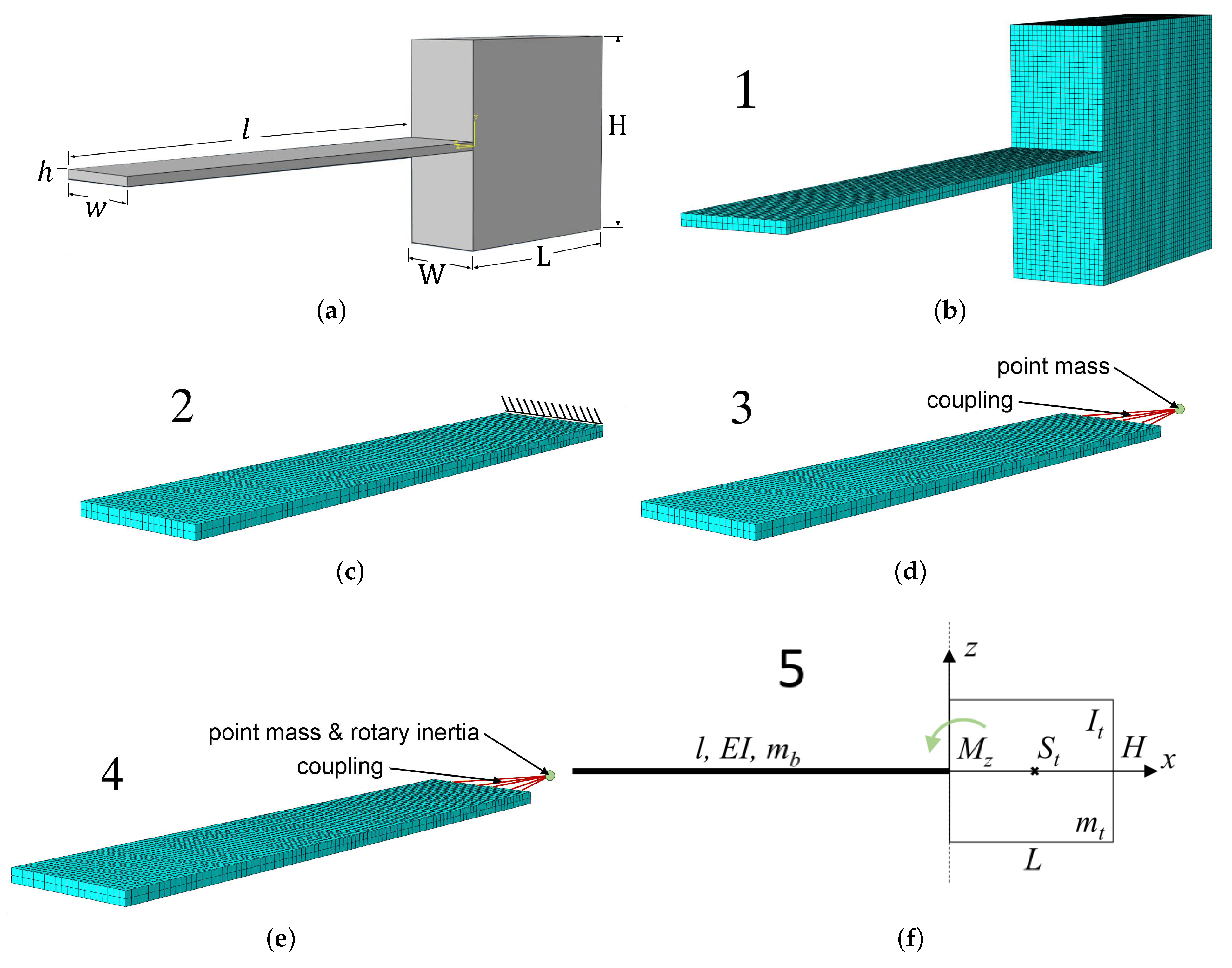
2. Model Descriptions

Following a short description of the test samples, three variations of the methodologies are presented: a finite element model, an experimental modal analysis, and finally an analytical model. In total, five prediction models are considered.

2.1. Test Samples

In the following, the influence of a significantly simplified boundary condition on finite element models is discussed. First, six reference structures consisting of a beam with a large mass attached to the free end are considered (see Figure 1a). The beam samples are made of steel with the material properties homogeneous and elastic were assumed. The large mass, also steel, is approximately 10-times the mass of the beam.

Various mass ratios were considered that could provide a limit on the minimum beam to large mass ratio; however, no definitive conclusions could be drawn below the mass ratio of 10 preferred here. The nominal values of the material and geometrical parameters with averaged deviation $\epsilon$ over six samples are given in

Table 1. The nominal values of the geometrical and material parameters with the averaged deviation $\epsilon$ over six samples.

Parameters (Steel Specimens)	1	2	3	4	5	6	Mean	Standard Deviation $\mathit{\epsilon }$
Length, l [m]	0.2001	0.2001	0.1999	0.2002	0.2000	0.2002	0.2001	$\pm 0.02\times {10}^{-3}$
Width, w [m]	0.0399	0.0399	0.0400	0.0400	0.0399	0.0400	0.0399	$\pm 0.02\times {10}^{-3}$
Thickness, h [m]	0.0040	0.0040	0.0041	0.0040	0.0040	0.0040	0.0040	$\pm 0.02\times {10}^{-3}$
Density, $\rho$ [kgm${}^{-3}$]	7700	7700	7700	7700	7700	7700	7700	$\pm 0.8$
Young’s modulus, E [GPa]	203.1	202.6	203.1	203.3	205.2	204.1	203.6	$\pm 4.7$
Poisson’s ratio, $\nu$ [-]	0.29	0.29	0.29	0.29	0.28	0.28	0.29	$\pm 0.01$

. The nominal value and uncertainty of the parameters related to the material properties is obtained by performing measurements with a parameter identification method described in [23].

The velocity of longitudinal $\left(c_l\right)$ and transversal $\left(c_t\right)$ waves in an elastic continuum are given by

$$c_l=\sqrt{\frac{E·(1-\nu )}{\varrho ·(1+\nu )·(1-2\nu )}}$$

(1)

and

$$c_t=\sqrt{\frac{E}{2\varrho ·(1+\nu )}},$$

(2)

respectively. Herein, $\varrho$ denotes the structure’s density. Transforming both equations yields two expressions for Young’s modulus E, i.e.,

$$E\left(c_l\right)=\frac{{c_l}^2·\varrho ·(1+\nu )·(1-2\nu )}{(1-\nu )}$$

(3)

and

$$E\left(c_t\right)=2·{c_t}^2·\varrho ·(1+\nu ).$$

(4)

Assuming that $E\left(c_l\right)=E\left(c_t\right)$ results in

$$\nu =\frac{2{c_t}^2-{c_l}^2}{2·({c_t}^2-{c_l}^2)}.$$

(5)

Given the longitudinal and transversal wave velocities $c_l$ and $c_t$, Poisson’s ratio $\nu$ can be easily obtained from Equation (5). For determining the Young’s modulus, Equation (3) and Equation (4) were evaluated, and their results were averaged, i.e., $E=1/2(E\left(c_l\right)+E\left(c_t\right))$. The ultrasonic measurements were performed using the 5-MHz ultrasonic module UT/Mate from Vogt ultrasonics and transducers. All measurements were taken in reflection mode, i.e., pulse-echo mode, on specimens with plane-parallel grinded surfaces. On each specimen, ten individual measurements were taken for both the longitudinal and transversal sound velocities.

The density was measured employing hydrostatic weighing using Archimedes’ principle. For this, a Mettler Toledo 204AG of 0.1-mg scale is used. Each specimen was first weighed in air, yielding $m_{\mathrm{air}}$, and afterward weighed in water, yielding $m_{\mathrm{water}}$. Given the two masses and the density of water ${\varrho }_{\mathrm{water}}$ and air ${\varrho }_{\mathrm{air}}$, the density $\varrho$ of the specimen can be calculated using Equation (6) without knowledge of the specimen’s volume.

$$\varrho =\frac{m_{\mathrm{air}}·({\varrho }_{\mathrm{water}}-{\varrho }_{\mathrm{air}})}{m_{\mathrm{air}}-m_{\mathrm{water}}}+{\varrho }_{\mathrm{air}}.$$

(6)

Five variations of an approximation for a large attachment are implemented (Figure 1). Four of these are derived from finite element analysis and the fifth is an analytical model. Each variation will be considered for its benefits and possible drawbacks.

2.2. Finite Element Models

The grid for the associated finite element model, as shown in Figure 1b, is a structured mesh using 20-node quadratic hexahedral elements, C3D20 (ABAQUS v6, [1]) and applying meshing guidelines according to Langer et al. [27,28]. A total of 54,000 elements were used, which corresponds to 236,541 nodes. This reference model (modelling approach 1) has no simplifications and ideal free–free boundary conditions. In the next step, three simplified finite element models are investigated (see Figure 1c–f).

For modelling approach 2, c.f. Figure 1c, the effect of the tip–mass was modelled as an ideal rigid clamping condition, which defines zero motion at this point. This is possibly the most common implementation in ABAQUS/CAE, which removes the complexity of modelling a tip-mass. This compares to an approximately infinite mass and infinite rotary inertia at the end-point. For more realistic models, two additional finite element models were investigated. Modelling approach 3, c.f. Figure 1d, approximates the tip-mass by an ideal free-tip mass, coupling a point mass to the beam’s end.

Extending this approach, modelling approach 4 additionally takes the rotary inertia into account. For both cases, the point mass is located at the centre of gravity of the 3D tip mass and is connected to the front surface of the beam via kinematic coupling. The rotary inertia $I_{\mathrm{t}}$ for the tip–mass is calculated by

$$I_{\mathrm{t}}=\frac{m_{\mathrm{t}}(L^2+H^2)}{12}+\frac{1}{4}{L}^2{m}_{\mathrm{t}}.$$

(7)

The modelling approaches 2, 3 and 4 include simplifications to reduce the degrees of freedom and, thus, the complexity of the numerical modal analysis. In addition to the simplifications, the finite element mesh for the beam was left unchanged and, hence, matched the reference model. In addition to the finite element models, Figure 1f shows an analytical Euler–Bernoulli beam model considering an ideal free-tip mass and the rotary inertia. This corresponds to modelling approach 5. The theoretical background is explained, and can be found in Section 2.4 for reference.

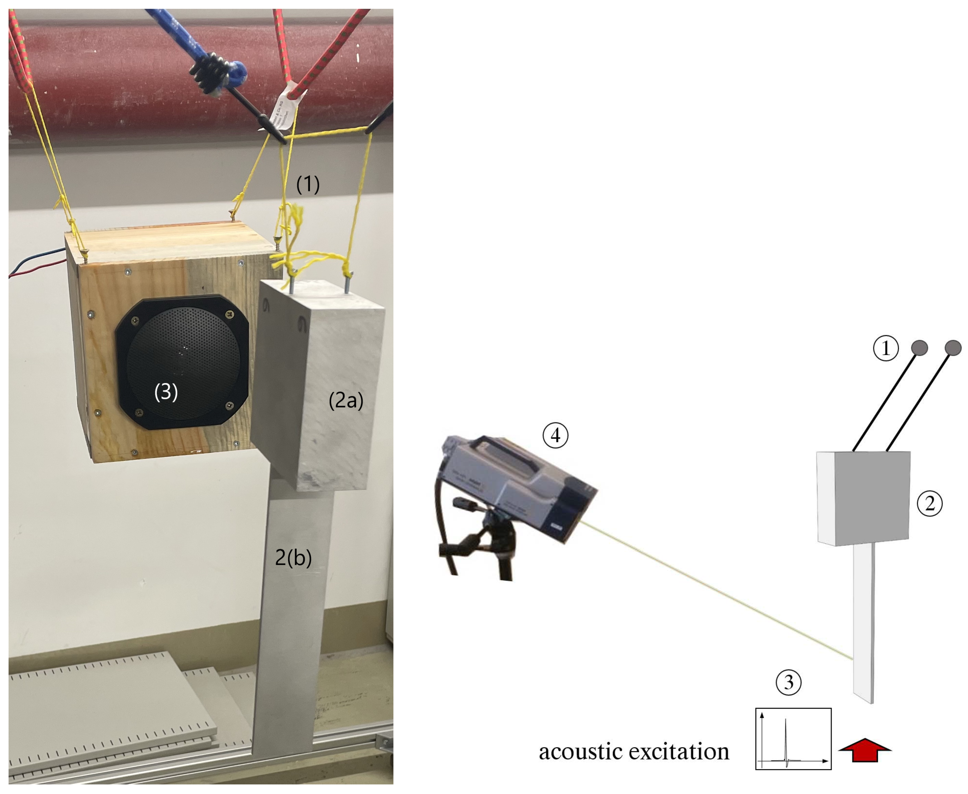
2.3. Experimental Modal Analysis

For the experimental modal analysis (EMA), a contact–free measurement setup using a laser Doppler vibrometer (PSV-400, Polytec, GmbH, Waldbronn, Germany) was used, c.f. Figure 2. The six specimens, each one a distinct body, appearing as a beam with a tip mass attached to the free end, were suspended on two elastic strings and were acoustically activated by a loudspeaker using a ramped sinusoidal sweep in the frequency range to $1\mathrm{kHz}$ with a sampling frequency of $f_s=4000\mathrm{cycles}/\mathrm{s}$.

Measurements were performed in an anechoic chamber to avoid the influence of acoustic reflections from the walls. A microphone measured the effective sound pressure generated by the loudspeaker to find the input value for the frequency response function (FRF). This procedure allows for extracting the eigenfrequencies of the structural modes and is, thus, sufficient for the presented study. However, when seeking to determine the modal damping parameters, a different technique for measuring the excitation has to be used. The deflection shape of each of the six specimens was measured by a laser Doppler vibrometer in front of the investigated structure.

By using a contact–free measurement setup, any artificial effect of the measurement equipment, e.g., the mass added by applying an accelerometer for measuring the deflection, is eliminated. Further, the suspension of the specimens was chosen such that the frequencies of the rigid body modes were at least one order of magnitude below the first eigenfrequency of interest. Therefore, the suspension can be adequately modelled by ideal free–free boundary conditions [29]. A review of different measurement techniques is provided, for example, by Ewins [29] and the International Organization for Standardization [30].

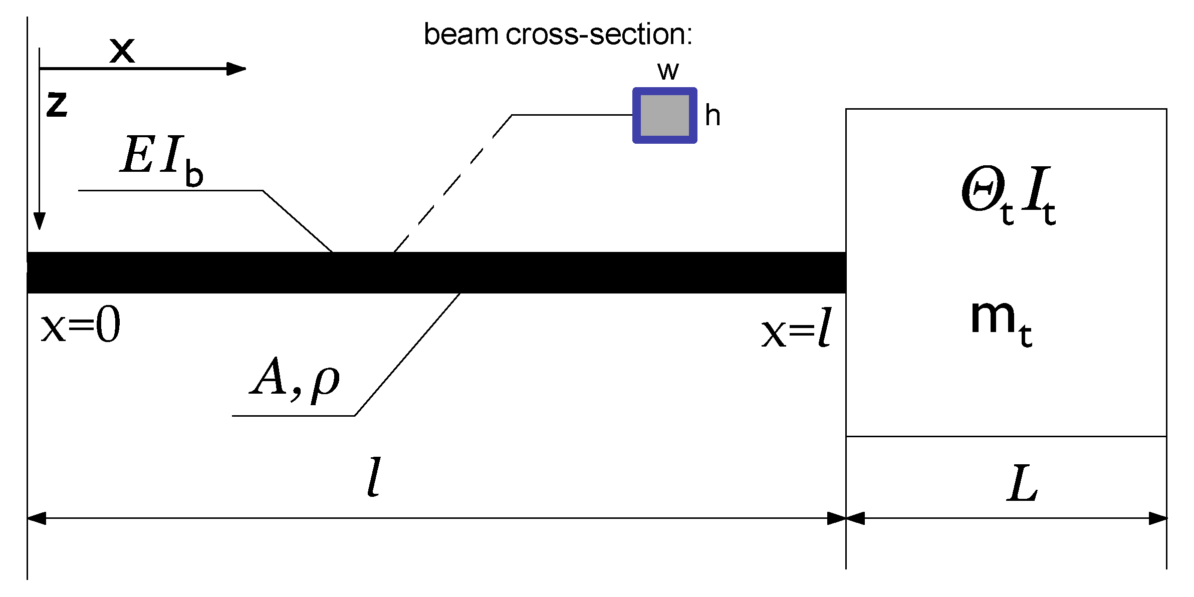
2.4. Analytical Theory

The Euler–Bernoulli beam theory is the most commonly used theory for simple vibration problems because of its simplicity due to reasonable approximations for many real physical problems. The theory is accurate for slender beams and for natural frequencies of the lower modes, see [27]. For this reason, the developed analytical formalism is based on the Euler–Bernoulli beam theory. We assume that the reader is familiar with the fundamental formulations of the Euler–Bernoulli model. Therefore, the authors refrain from including a detailed description here but refer the reader to the ample literature available, such as [31,32,33,34]. However, the basic assumptions of the Euler–Bernoulli theory should be mentioned as follows:

(i)

One of the spatial dimensions is significantly larger than the other two.

(ii)

The material behaves according to Hooke’s law.

(iii)

The Poisson effect is neglected.

(iv)

The angle of rotation is small; hence, the small angle assumption holds. The transverse displacements and cross-section rotations are small. Hence, the formulations are geometrically linear.

(v)

Cross-sections remain perpendicular to the neutral axes after deformation.

(vi)

The rotational inertia of the cross-sections is neglected.

Figure 3 shows the parameters of the one-dimensional model to develop the analytical formula to calculate eigenfrequencies for the bending modes.

The equation of motion for free vibrations according to the Euler–Bernoulli theory is given as:

$$\frac{{\partial }^{4}W(x,t)}{\partial x^4}+\frac{\rho A}{E{I}_{\mathrm{b}}}\frac{{\partial }^{2}W(x,t)}{\partial t^2}=0,$$

(8)

where $W(x,t)$ is the transverse displacement in z direction at the point x and the time t. Considering the freely supported structure presented in Figure 3, interface boundary conditions (at $x=l$) can be formulated for the simplified model in terms of relating the bending moment and shear forces at the beam end and equivalent terms for the tip-mass, see Andrews and Shillor [35],

$${\left[m_{\mathrm{t}}\frac{{\partial }^{2}W(x,t)}{\partial t^2}-E{I}_{\mathrm{b}}\frac{{\partial }^{3}W(x,t)}{\partial x^3}\right]}_{x=l}=0,{\left[{\theta }_{\mathrm{t}}\frac{{\partial }^{3}W(x,t)}{\partial t^2\partial x}+E{I}_{\mathrm{b}}\frac{{\partial }^{2}W(x,t)}{\partial x^2}\right]}_{x=l}=0$$

(9)

and at the left hand edge

$${\left.\frac{{\partial }^{2}W(x,t)}{\partial x^2}\right|}_{x=0}=0,{\left.\frac{{\partial }^{3}W(x,t)}{\partial x^3}\right|}_{x=0}=0.$$

(10)

Using the standard separation of variables applied to $W(x,t)$ into two functions:

$$W(x,t)=\varphi \left(x\right)T\left(t\right).$$

(11)

and the following fourth-order differential–equation, which describes free flexural vibrations of a thin beam follows from Equation (8):

$$E{I}_{\mathrm{b}}\varrho A\frac{d^4\varphi \left(x\right)}{d{x}^4}+{\left(\frac{\lambda }{l}\right)}^4\varphi \left(x\right)=0,$$

(12)

where $\lambda$ is a positive constant.

It is well established that the spatial solutions of the homogeneous Equation (8) can be considered as flexural mode shapes:

$$\varphi \left(x\right)=Acos{\lambda }_n\frac{x}{l}+Bsin{\lambda }_n\frac{x}{l}+Ccosh{\lambda }_n\frac{x}{l}+Dsinh{\lambda }_n\frac{x}{l},n\ge 1$$

(13)

where ${\lambda }_n$ and A, B, C, and D are the eigenvalues and mode shape parameters. In Equation (13)

$${\lambda }_n^4=\frac{\varrho A}{E{I}_{\mathrm{b}}}{\omega }_n^2{l}^4.$$

(14)

is the well-known relation between eigenvalues and the natural frequency of vibrations, $\omega$.

Employing the notation $c\left(\lambda \right)=cos\left(\lambda \right),s\left(\lambda \right)=sin\left(\lambda \right),ch\left(\lambda \right)=cosh\left(\lambda \right),sh\left(\lambda \right)=sinh\left(\lambda \right)$, and after some standard algebraic manipulations, the characteristic equation follows:

$$\begin{array}{cc}\hfill & C{}_T\left(\lambda \right)=\frac{{\lambda }^4{m}_{\mathrm{t}}{\theta }_{\mathrm{t}}}{l^2{m}_{\mathrm{b}}^2}(1+c\left(\lambda \right)ch\left(\lambda \right))+\frac{{\lambda }^3{\theta }_{\mathrm{t}}}{l^2{m}_{\mathrm{b}}^2}(c\left(\lambda \right)sh\left(\lambda \right)+ch\left(\lambda \right)s\left(\lambda \right))\hfill \\ \hfill & -\frac{\lambda m_{\mathrm{t}}}{m_{\mathrm{b}}}(c\left(\lambda \right)sh\left(\lambda \right)-ch\left(\lambda \right)s\left(\lambda \right))-c\left(\lambda \right)ch\left(\lambda \right)+1=0.\hfill \end{array}$$

(15)

For the limiting cases $m_{\mathrm{t}}\to 0$ and ${\theta }_{\mathrm{t}}\to 0$, the characteristic equation reduces to

$$\begin{array}{c}\hfill c\left(\lambda \right)ch\left(\lambda \right)-1=0,\end{array}$$

(16)

which applies to a beam with ideal free–free boundary conditions.

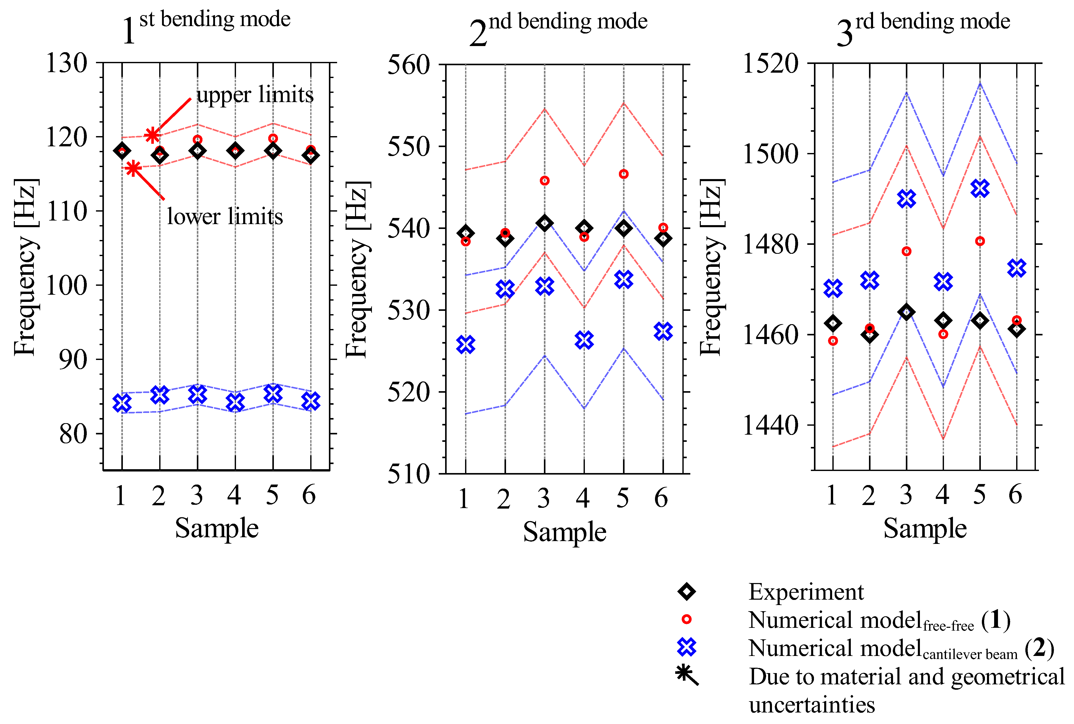
3. Results and Discussion

In this section, a comparison between the experimental and simulation results is presented. In the first step, the results gained through experimental modal analyses based on the setup shown in Figure 2 are compared to the results determined by numerical modal analyses using modelling approach 1, i.e., ideal free–free boundary conditions as shown in Figure 1b, and modelling approach 2, i.e., ideal rigid–clamped conditions, c.f. Figure 1c.

The results were determined for each of the six test specimens, taking the individual geometry parameters and the corresponding uncertainty into account. This first comparison is presented in Figure 4. The relative deviation of the averaged experimentally determined natural frequencies between samples is $4.0\%$, $3.9\%$, and $3.9\%$ for the first three bending modes. This deviation indicates that a high uncertainty in vibration characterisation cannot be ruled out for physical structures that are produced in a single unit of production.

The two simplified finite element models are now investigated, taking only the first specimen into account. The first specimen representing the closest to the “mean” for the first natural frequencies. The idea here is to compare the uncertainty of the analytical models with measurements but not to compare uncertainties in both or, moreover, to determine any conclusions with measurement uncertainties. Hence, we go no further except to bear in mind the general $4.0\%$ uncertainty in the first three measured natural frequencies.

Now, we proceed with the finite element models, which include a modelling approach 3 with a tied coupling of a point mass as illustrated in Figure 1d and a modelling approach 4 with a tied coupling of both a point mass and a rotary inertia as illustrated in Figure 1e. The corresponding results are compared to results based on the modelling approach 5, i.e., using the analytical solution of the simplified beam model shown in Figure 1e, as well as to the experimental results of the corresponding specimen. For the comparisons, an averaged relative error $\epsilon$ was calculated for the first three eigenfrequencies over m specimens using

$$\epsilon =\frac{1}{m}\sum _{i=1}^m\left({\displaystyle \frac{f_{\mathrm{i}}}{f_{{\exp }_{\mathrm{i}}}}}-1\right)·100\%,$$

(17)

where $f_{\exp }$ is the eigenfrequency determined by the experiments and f is the corresponding eigenfrequency obtained by the numerical model. The averaged relative deviation between the results determined by the numerical models and the experimental measurements is given in

Table 2. Averaged relative deviation $\epsilon$ from the finite element models to the experiment for the eigenfrequencies of the first three bending modes. ${\mathrm{FE}}_{\mathrm{free}-\mathrm{free}}$ (1): reference model without simplifications. ${\mathrm{FE}}_{\mathrm{free}-\mathrm{clamped}}$ and (2): simplified finite element model of the beam with ideal-rigid clamping.

Mode	Experiment [Hz]	${\mathbf{FE}}_{\mathbf{free}-\mathbf{free}}$ (1)	${\mathbf{FE}}_{\mathbf{free}-\mathbf{clamped}}$ (2)
$1\mathrm{st}$	118	$0.6\%$	$-28.2\%$
$2\mathrm{nd}$	540	$0.4\%$	$-1.8\%$
$3\mathrm{rd}$	1462	$0.3\%$	$1.1\%$

and

Table 3. Relative deviation of the results determined by the simplified finite element models and the analytical solution to the experimental results of the eigenfrequencies of the first three bending modes. Only the first specimen is taken into account.

Mode	Experiment [Hz]	FE${}_{\mathbf{free}-\mathbf{tip}\mathbf{mass}}$ (3)	FEfree-tip mass & inertia (4)	${\mathbf{Analytic}}_{\mathbf{free}-\mathbf{free}}$ (5)
$1\mathrm{st}$	118	$112.7\%$	$0.8\%$	$2.9\%$
$2\mathrm{nd}$	540	$63.1\%$	$1.5\%$	$0.6\%$
$3\mathrm{rd}$	1462	$33.7\%$	$1.7\%$	$0.7\%$

for the first and second comparison, respectively.

Clearly, from Figure 4, modelling the specimen in full detail with three dimensional solid elements and applying free–free boundary conditions is a valid modelling approach for engineering purposes. The numerical results of this reference model ${\mathrm{FE}}_{\mathrm{free}-\mathrm{free}}$ share a high level of agreement with the experimental results. The deviation was lower than $1\%$ over the whole frequency range as indicated in Table 2.

In contrast, the modelling approach 2, i.e., replacing the tip-mass at the end of the specimen with ideal clamped boundary conditions, yielded insufficient results. Even within the bounds of experimental uncertainty, which are largely acceptable for the second and third bending mode, the first bending mode was not correctly identified by this reduced numerical model ${\mathrm{FE}}_{\mathrm{free}-\mathrm{clamped}}$. The arithmetically averaged relative deviations for the eigenfrequencies of the first three bending modes were $-28.2\%$, $-1.8\%$, and $1.1\%$, respectively.

In Figure 4, an envelope identifying the upper and lower limits around the mean values of the eigenfrequencies indicates the deviation due to the material and geometrical uncertainties. These limits were determined by applying the Interval Method, the details of which can be found in c.f. [23,24,25]. It is clear that the uncertainty range of modelling approach 2 (blue) did not overlap the uncertainty range of modelling approach 1 (red) for the first bending eigenfrequency. Hence, there is little likelihood of predicting the first “true” bending mode from a simplified free–clamped model. However, the uncertainty ranges for the two modelling approaches do overlap for eigenfrequencies of the second and third bending mode. The consequence is that, especially for low frequencies, it is not recommended to use a free–clamped boundary condition to approximate the effect of an attached, large mass.

To understand the high deviation for the first eigenfrequency of bending modes, we take a closer look at the associated mode shapes. Figure 5 shows the mode shapes for the first three bending modes of the cantilever beam and the simple beam with the tip mass. In the second and third bending modes, the mode shapes are nearly identical. This means, that the location of the two end–nodes for the second mode and the three nodes for the third mode are situated at nearly the same point.

This is not the case for the first bending mode. Although both mode shapes have exactly one node, as expected, the position of the nodes is not the same. Although it is difficult to assess directly from Figure 5a, for the cantilever beam, the node is located at the ideal rigid constraint, whereas, for the beam with the tip mass, the node is located slightly away from the boundary, i.e., closer to the centre of the beam.

Having identified modelling approach 2 as insufficient, the focus is set on the approaches 3, 4 and 5, c.f. Figure 1. In this case, only one specimen is taken into account. Figure 6 shows that modelling approach 3, i.e., replacing the tip-mass at the end of the beam by a coupling of a point mass, yielded the highest deviation over the whole frequency range. For the first natural frequency, the deviation even exceeded $100\%$. Thus, taking only the tip mass into account and neglecting the rotary inertia is not a valid modelling approach. However, when using modelling approach 4, i.e., adding the rotary inertia of the tip-mass, far better results were achieved.

The relative deviation between the numerical results and the experimental results was below $2\%$ for all considered eigenfrequencies. In the case of modelling approach 5, i.e., the analytic model ${\mathrm{Analytic}}_{\mathrm{free}-\mathrm{free}}$ assuming free–free boundary conditions, the highest deviation was found at the first eigenfrequency with $2.9\%$. For the second and third eigenfrequency, the deviations to the experiment were less than $1\%$. Thus, both the finite element model with the coupling of the point mass and rotary inertia as well as the analytical model yielded sufficiently accurate results.

As a last step, we studied the effect of the uncertainties of the geometrical and material parameters for the tip mass. In this case the large attachment. Using the finite element model FE_{free-tip mass & inertia}, these uncertainties were included into the model by changing the point mass and rotary inertia values accordingly. Based on the values given in Table 1, a relative deviation from the mean value, or expected value, of the determined eigenfrequencies of less than $\pm 0.8\%$ was found. Therefore, we conclude that the effect of uncertainties, which describe the tip mass in the model, can be neglected in the modelling process.

4. Conclusions

In this paper, we presented a study of five different approaches for reducing the computational effort for a full finite element modal analysis when facing structures where flexible subcomponents are attached to other heavier subcomponents. The approaches include a reference model without any simplifications and finite element models where the heavy subcomponent is replaced by ideal rigid clamping, by a free-tip mass model or by a free-tip mass model with an additional rotary inertia. Furthermore, an analytic approach based on the Euler–Bernoulli beam theory was chosen.

The accuracy of the presented modelling approaches was assessed by comparing the corresponding numerical results with experimental results based on the eigenfrequencies of the first three bending modes. Seeking to give generic results, a monolithic beam-like structure with ideal free–free boundary conditions and a tip mass attached to one end of the beam were considered for comparison in this work. This latter configuration permits an in-depth comparison and uncertainty quantification due to the low cost of calculations and allows for a simplified model validation process. Although a rather simple model was chosen, the conclusions of the presented studies can be extended to complex structures.

The investigations showed that, beyond the first bending mode, the ideal rigid boundary condition provides a good approximation. An error analysis between numerical and experimental results showed that, for the second and third bending mode, the deviations were only $2\%$ and $1\%$, respectively, while this value was as high as $28\%$ for the first bending mode. This indicates that, for this mode, the model was very sensitive to the boundary conditions, and applying a small change will affect the associated mode shapes significantly. In summary, at low natural frequencies, the mode shapes were sensitive to the ideal clamping boundary conditions, and these conditions must be chosen carefully to achieve satisfactory results.

However, this does not hold for all of the other modelling approaches. Especially when replacing the tip-mass by coupling a corresponding point mass and rotary inertia to the free end, sufficiently accurate results can be achieved for all eigenfrequencies of the three bending modes. Based on this approach, relative errors of less than $2\%$ were achieved, proving it as the most favourable modelling approach if an analytical model is not feasible. Given that the mass-ratio of the attached mass to the beam, was rather low in our study, $12.5$, higher mass ratio masses should lead to similar results at the first three and higher natural frequencies. General but important remarks regarding simulation models that include large lumped-masses as secondary components, are:

• A full finite element model for all the components, including large heavy masses, using ideal-free conditions for the model is better suited where comparisons to experimental results are necessary, given that sufficient computer memory resources are available.
• For the simplification of a large attached mass by an ideal clamped condition in a finite element model, a very high mass ratio is necessary, although the end results can still be quite poor even for the primary first bending mode.
• It is commonly known, and was demonstrated here, that an analytical model can yield satisfactory results for a beam with an attached tip–mass, when the structure is beam–like.
• Reduced size modelling by a finite element approach using only an offset point-mass term for simplification can be easily improved upon by adding a rotary inertia term. This increases the accuracy and reduces computer resources; however, choosing a suitable rotary inertia term has its own challenges.

References

1. Simulia, D.S. ABAQUS V6.10 Documentation; Dassault Systèmes: Providence, RI, USA, 2010. [Google Scholar]
2. Bathe, K.J. Finite Element Procedures; Prentice-Hall: New Jersey, NJ, USA, 1996. [Google Scholar]
3. Zienkiewicz, O.C.; Taylor, R.L. The Finite Element Method Volume 1: Basic Formulation and Linear Problems; MacGraw-Hill Book Company: New York, NY, USA, 1989. [Google Scholar]
4. Zienkiewicz, O.C.; Taylor, R.L. The Finite Element Method Volume 2: Solid and Fluid Mechanics, Dynamics and Non-Linearity; MacGraw-Hill Book Company: New York, NY, USA, 1991. [Google Scholar]
5. Szabo, B.; Babuška, I. Finite Element Analysis; John Wiley & Sons, Inc.: New York, NY, USA, 1991. [Google Scholar]
6. Ghanem, R.G. Uncertainty Quantification in Computational and Prediction Science. Int. J. Numer. Methods Eng. 2009, 80, 671–672. [Google Scholar] [CrossRef]
7. Sargent, G. Verification and Validation of Simulation Models. In Proceedings of the Winter Simulation Conference, Orlando, FL, USA, 4 December 2005; pp. 53–59. [Google Scholar]
8. Li, R.; Ghanem, R. Adaptive polynomial chaos expansions applied to statistics of extremes in nonlinear random vibration. Probab. Eng. Mech. 1998, 13, 125–136. [Google Scholar] [CrossRef]
9. Lucor, D.; Su, C.H.; Karniadakis, G.E. Generalized polynomial chaos and random oscillators. Int. J. Numer. Methods Eng. 2004, 60, 571–596. [Google Scholar] [CrossRef]
10. Soize, C. A comprehensive overview of a non–parametric probabilistic approach of model uncertainties for predictive models in structural dynamics. J. Sound Vib. 2005, 288, 623–652. [Google Scholar] [CrossRef] [Green Version]
11. Sepahvand, K.; Marburg, S.; Hardtke, H.J. Stochastic free vibration of orthotropic plates using generalized polynomial chaos expansion. J. Sound Vib. 2012, 331, 167–179. [Google Scholar] [CrossRef]
12. Marburg, S.; Beer, H.J.; Gier, J.; Hardtke, H.J.; Rennert, R.; Perret, F. Experimental verification of structural–acoustic modelling and design optimization. J. Sound Vib. 2002, 252, 591–615. [Google Scholar] [CrossRef]
13. Marc, M.; Soize, C.; Avalos, J.D. Nonparametric stochastic modeling of structures with uncertain boundary, conditions/coupling between substructures. AIAA J. 2013, 51, 1298–1308. [Google Scholar]
14. Ritto, T.G.; Sampaio, R.; Aguiar, R.R. Uncertain boundary condition Bayesian identification from experimental data: A case study on a cantilever beam. Mech. Syst. Signal Process. 2016, 68–69, 176–188. [Google Scholar] [CrossRef]
15. Ewins, D. Exciting vibrations: The role of testing in an era of supercomputers and uncertainties. Meccanica 2016, 51, 3241–3258. [Google Scholar] [CrossRef] [Green Version]
16. Alvin, K.; Oberkampf, W.; Diegert, K.; Rutherford, B. Uncertainty quantification in computational structural dynamics: A new paradigm for model validation. In Proceedings of the 16th International Modal Analysis Conference, Santa Barabara, CA, USA, 2–5 February 1998; Volume 2, pp. 1191–1198. [Google Scholar]
17. Oberkampf, W.L.; DeLand, S.M.; Rutherford, B.M.; Diegert, K.V.; Alvin, K.F. Error and uncertainty in modeling and simulation. Reliab. Eng. Syst. Saf. 2002, 75, 333–357. [Google Scholar] [CrossRef]
18. Smith, R.C. Uncertainty Quantification: Theory, Implementation, and Applications; Siam: Philadelphia, PA, USA, 2013; Volume 12. [Google Scholar]
19. Sullivan, T.J. Introduction to Uncertainty Quantification; Springer: Cham/Heidelberg, Germany, 2015; Volume 63. [Google Scholar]
20. Marburg, S.; Dienerowitz, F.; Fritze, D.; Hardtke, H.J. Case studies on structural-acoustic optimization of a finite beam. Acta Acust. United Acust. 2006, 92, 427–439. [Google Scholar]
21. Inman, D.J.; Erturk, A. Piezoelectric Energy Harvesting; John Wiley & Sons: New York, NY, USA, 2011. [Google Scholar]
22. Kirk, C.L.; Wiedemann, S.M. Natural Frequencies and Mode Shapes of a Free-Free Beam with Large End Masses. J. Sound Vib. 2002, 254, 939–949. [Google Scholar] [CrossRef]
23. Langer, P.; Sepahvand, K.; Guist, C.; Bär, J.; Peplow, A.; Marburg, S. Matching experimental and three dimensional numerical models for structural vibration problems with uncertainties. J. Sound Vib. 2018, 417, 294–305. [Google Scholar] [CrossRef]
24. Neumaier, A. Interval Methods for Systems of Equations; Cambridge University Press: Cambridge, UK, 1990. [Google Scholar]
25. Moore, R.E. Methods and Applications of Interval Analysis; Society for Industrial and Applied Mathematics: Philadelphia, PA, USA, 1987. [Google Scholar]
26. Elishakoff, I.; Soret, C. Remedy to overestimation of classical interval analysis: Analysis of beams with uncertain boundary conditions. Shock Vib. 2013, 20, 143–156. [Google Scholar] [CrossRef]
27. Langer, P.; Sepahvand, K.; Marburg, S. Uncertainty quantification in analytical and finite element beam models using experimental data. In Proceedings of the 9th International Conference on Structural Dynamics, EURODYN 2014, Porto, Portugal, 30 June–2 July 2014. [Google Scholar]
28. Langer, P.; Maeder, M.; Guist, C.; Krause, M.; Marburg, S. More Than Six Elements Per Wavelength: The Practical Use of Structural Finite Element Models and Their Accuracy in Comparison with Experimental Results. J. Comput. Acoust. 2017, 25, 1750025. [Google Scholar] [CrossRef]
29. Ewins, D.J. Modal Testing: Theory and Practice; Research Studies Press: Letchworth, Hertfordshire, UK, 1984. [Google Scholar]
30. ISO 7626-1:2011: Methods for the Experimental Determination of Mechanical Mobility; Parts 1–5. Technical Report; International Organisation for Standardization: Geneva, Switzerland, 2011.
31. Han, S.M.; Benaroya, H.; Wei, T. Dynamics of transversely vibrating beams using four engineering theories. J. Sound Vib. 1999, 225, 935–988. [Google Scholar] [CrossRef] [Green Version]
32. Benaroya, H.; Nagurka, M.L. Mechanical Vibration: Analysis, Uncertainties, and Control; CRC Press: Boca Raton, FL, USA, 2017. [Google Scholar]
33. Inman, D. Engineering Vibration; Pearson Education: Upper Saddle River, NJ, USA, 2008. [Google Scholar]
34. Meirovitch, L. Elements of Vibration Analysis, 2nd ed.; McGrawHill: New York, NY, USA, 1986. [Google Scholar]
35. Andrews, K.; Shillor, M. Vibrations of a beam with a damping tip body. Math. Comput. Model. 2002, 35, 1033–1042. [Google Scholar] [CrossRef]
Figure 1. Investigated structure and finite element models. (a) Geometry of the specimens. Coordinate axes follow: length of beam (l) x–axis, beam thickness (h) z–axis, and beam width (w) y–axis. (b) Finite element model 1 of the real structure with ideal free–free boundary condition—reference model. (c) Simplified finite element model 2 with ideal rigid clamping. (d) Simplified finite element model 3 with ideal free-tip mass modelling. (e) Simplified finite element model 4 with ideal free-tip mass and rotary inertia modelling. (f) Euler–Bernoulli beam model 5 with ideal free-tip mass and rotary inertia modelling.
Applsci 11 05428 g001
Figure 2. Image and sketch of the experimental setup showing: elastic strings (1), specimen mass (2a), specimen beam (2b), acoustic excitation (3), and laser Doppler vibrometer (4).
Applsci 11 05428 g002
Figure 3. Parameters of the one-dimensional model. m t : mass of the tip mass. I t : area moment of inertia of the tip mass about the axis of bending. I b : area moment of inertia of the beam about the axis of bending. A: cross-section area. θ t : mass moment of inertia of the tip mass about the axis of bending. The nominal geometrical and material parameters are the same as in Section 2.1.
Applsci 11 05428 g003
Figure 4. Two numerical model finite element results compared to experiments for the eigenfrequencies related to the first three bending modes. Experiment: contact-free measurement setup Figure 1a.
Applsci 11 05428 g004
Figure 5. Mode shapes of the cantilever beam and the simple beam with a tip mass attached to the free end. (a) First bending mode. (b) Second bending mode. (c) Third bending mode.
Applsci 11 05428 g005
Figure 6. Experimental and further lumped-parameter finite element and analytic simulation results for the eigenfrequencies related to the first three bending modes of the first specimen. Experiment: contact-free measurement setup. Modelling approach 3: tied coupling of a point mass. Modelling approach 4: tied coupling of a point mass and a rotary inertia. Modelling approach 5: Analytical description of a simplified model according to the Euler–Bernoulli theory.
Applsci 11 05428 g006