
MR Images, Brain Lesions, and Deep Learning


1
Departamento de Química y Ciencias Exactas, Sección Fisicoquímica y Matemáticas, Universidad Técnica Particular de Loja, San Cayetano Alto s/n, Loja 11-01-608, Ecuador
2
Theoretical and Experimental Epistemology Lab, School of Optometry and Vision Science, University of Waterloo, Waterloo, ON N2L3G1, Canada
3
Instituto de Instrumentación para Imagen Molecular (i3M) Universitat Politècnica de València—Consejo Superior de Investigaciones Científicas (CSIC), E-46022 Valencia, Spain
4
Departments of Physics, Electrical and Computer Engineering and Systems Design Engineering, University of Waterloo, Waterloo, ON N2L3G1, Canada
*
Author to whom correspondence should be addressed.
Appl. Sci. 2021, 11(4), 1675; https://doi.org/10.3390/app11041675
Submission received: 20 January 2021
/
Revised: 8 February 2021
/
Accepted: 8 February 2021
/
Published: 13 February 2021
(This article belongs to the Special Issue Deep Signal/Image Processing: Applications and New Algorithms)
Abstract
:Featured Application
This review provides a critical review of deep/machine learning algorithms used in the identification of ischemic stroke and demyelinating brain diseases. It evaluates their strengths and weaknesses when applied to real world clinical data.
Abstract
Medical brain image analysis is a necessary step in computer-assisted/computer-aided diagnosis (CAD) systems. Advancements in both hardware and software in the past few years have led to improved segmentation and classification of various diseases. In the present work, we review the published literature on systems and algorithms that allow for classification, identification, and detection of white matter hyperintensities (WMHs) of brain magnetic resonance (MR) images, specifically in cases of ischemic stroke and demyelinating diseases. For the selection criteria, we used bibliometric networks. Of a total of 140 documents, we selected 38 articles that deal with the main objectives of this study. Based on the analysis and discussion of the revised documents, there is constant growth in the research and development of new deep learning models to achieve the highest accuracy and reliability of the segmentation of ischemic and demyelinating lesions. Models with good performance metrics (e.g., Dice similarity coefficient, DSC: 0.99) were found; however, there is little practical application due to the use of small datasets and a lack of reproducibility. Therefore, the main conclusion is that there should be multidisciplinary research groups to overcome the gap between CAD developments and their deployment in the clinical environment.
1. Introduction
There are estimated to be as many as a billion people worldwide [1] affected by peripheral and central neurological disorders [1,2]. Some of these disorders include brain tumors, Parkinson’s disease (PD), Alzheimer’s disease (AD), multiple sclerosis (MS), epilepsy, dementia, neuroinfectious, stroke, and traumatic brain injuries [1]. According to the World Health Organization (WHO), ischemic stroke and “Alzheimer disease with other dementias” are the second and fifth major causes of death, respectively [2].
Biomedical images give fundamental information necessary for the diagnosis, prognosis, and treatment of different pathologies. Hence, neuroimaging plays a fundamental role in understanding how the brain and the nervous system function [3] and discover how structural or functional anatomical alteration is correlated with different neurological disorders [4] and brain lesions. Currently, research on artificial intelligence (AI) and diverse techniques of imaging constitutes a crucial tool for studying the brain [5,6,7,8,9,10,11] and aids the physician to optimize the time-consuming tasks of detection and segmentation of brain anomalies [12] and also to better interpret brain images [13] and analyze complex brain imaging data [14].
In terms of neuroimaging of both normal tissues and pathologies, there are different modalities, namely (1) computed tomography (CT) and magnetic resonance imaging (MRI), which are commonly used for the structural visualization of the brain; (2) positron emission tomography (PET), used principally for physiological analysis; and (3) single-photon emission tomography (SPECT) and functional MRI, which are used for functional analysis of the brain [15].
MRI and CT are preferred by radiologists to understand brain pathologies [12]. Due to continual advancements in MRI technology, it considered to be a promising tool that can elucidate the brain structure and function [3], e.g., brain MR image resolution has grown by leaps and bounds since the first MR image acquisition [16]. Because of this reason, this modality is frequently used (more than CT) to examine anatomical brain structures, perform visual inspection of cranial nerves, and examine abnormalities of the posterior fossa and spinal cord [17]. Another advantage of MRI compared to CT is that MRI is less susceptible to artifacts in the image [18].
In addition, MR image analysis is useful different tasks, e.g., lesion detection, lesion segmentation, tissue segmentation, and brain parcellation on neonatal, infant, and adult subjects [4,5]. In this work, we discuss MR image processing to detect, segment, and classify white matter hyperintensities (WMHs) using techniques of artificial intelligence. Ghafoorian et al. [19] state that WMHs are seen in MRI studies of neurological disorders like multiple sclerosis, dementia, stroke, cerebral small-vessel disease (SVD), and Parkinson’s disease [19,20].
According to Leite et al. [20], due to a lack of pathological studies, the etiology of WMHs is frequently proposed to be of an ischemic or a demyelinating nature. A WMH is termed ischemia if caused by an obstruction of a blood vessel, and a WMH is considered to be demyelinating when there is an inflammation that causes destruction and loss of the myelin layer and compromises neural transmission [20,21,22], and this type of WMH is often related to multiple sclerosis (MS) [8,22] (Figure 1).
A stroke occurs when the blood flow to an area of the brain is interrupted [21,23]. There are three types of ischemic stroke according to the Bamford clinical classification system [24]: (1) partial anterior circulation syndrome (PACS), where the middle/anterior cerebral regions are affected; (2) lacunar anterior circulation syndrome (LACS), where the occlusion is present in vessels that provide blood to the deep-brain regions; and (3) total anterior circulation stroke (TACS), when middle/anterior cerebral regions are affected due to a massive brain stroke [24,25]. Ischemic stroke is a common cerebrovascular disease [1,26,27] and one of the principal causes of death and disability in low- and middle-income countries [1,4,6,7,27,28,29]. In developed countries, brain ischemia is responsible for 75–80% of strokes, and 10–15% are attributed to a hemorrhagic brain stroke [4,25].
A demyelination disease is described as the loss of myelin with relative preservation of axons [8,22,29]. Love [22] notes that there are demyelinating diseases in which axonal degeneration occurs first and the degradation of myelin is secondary [7,22]. Accurate diagnosis classifies the demyelinating diseases of the central nervous system (CNS) according to the pathogenesis into “demyelination due to inflammatory processes, demyelination caused by developed metabolic disorders, viral demyelination, hypoxic-ischemic forms of demyelination and demyelination produced by focal compression” [22].
The inflammatory demyelination of the CNS is the principal cause of the common neurological disorder multiple sclerosis (MS) [8,19,20,22,30], which affects the central nervous system [31] and is characterized by lesions produced in the white matter (WM) [32] of the brain and affects nearly 2.5 million people worldwide, especially young adults (ages 18–35 years) [4,30,31].
The detection, identification, classification, and diagnosis of stroke is often based on clinical decisions made using computed tomography (CT) and MRI [33]. Using MRI, it is possible to detect the presence of little infarcts and assess the presence of a stroke lesion in the superficial and deep regions of the brain with more accuracy. This is because the area of the stroke region is small and is clearly visible in MR images compared to CT [4,21,25,26,28,34]. The delimitation of the area plays a fundamental role in the diagnosis since it is possible to misdiagnose stroke as other disorders [35,36], e.g., glioma lesions and demyelinating diseases [19,20].
For identifying neurological disorders like stroke and demyelinating disease, the manual segmentation and delineation of anomalous brain tissue is the gold standard for lesion identification. However, this method is very time consuming and specialist experience dependent [25,37], and because of these limitations, automatic detection of neurological disorders is necessary, even though it is a complex task because of data variability, e.g., in the case of ischemic stroke lesions, data variability could include the lesion shape and location, and factors like symptom onset, occlusion site, and patient differences [38].
In the past few years, there has been considerable research in the field of machine learning (ML) and deep learning (DL) to create automatic or semiautomatic systems, algorithms, and methods that allow detection of lesions in the brain, such as tumors, MS, stroke, glioma, AD, etc. [4,6,8,9,10,26,28,30,36,39,40,41,42,43,44,45,46,47,48]. Different studies demonstrate that deep learning algorithms can be successfully used for medical image retrieval, segmentation, computer-aided diagnosis, disease detection, and classification [49,50,51]. However, there is much work to be done to develop accurate methods to get results comparable to those of specialists [43].
This critical review summarizes the literature on deep learning and machine learning techniques in the processing, segmentation, and detection of features of WMHs found in ischemic and demyelinating diseases in brain MR images.
The principal research questions asked here are:
- Why is research on the algorithms to identify ischemia and demyelination through the processing of medical images important?
- What are the techniques and methods used in developing automatic algorithms for detection of ischemia and demyelinating diseases in the brain?
- What are the performance metrics and common problems of deep learning systems proposed to date?
This paper is organized as follows. Section 2 gives an outline of the literature review selection criteria. Section 3 describes the principal machine learning and deep learning methods used in this application, Section 4 summarizes the principal constraints and common problems encountered in these CAD systems, and we conclude Section 5 with a brief discussion.
2. The Literature Review: Selection Criteria
The literature review was conducted using the recommendations given by Khan et al. [52], the methodology proposed by Torres-Carrión [53,54], and the protocol proposed by Moher et al. [55]. The preferred reporting items for systematic reviews and meta-analyses (PRISMA) flow diagram [55] is shown in Figure 2.
We generated and analyzed bibliometric maps and identified clusters and their reference networks [56,57]. We also used the methods given in [58,59] to identify the strength of the research, as well as authors and principal research centers that work with MR images and machine/deep learning for the identification of brain diseases.
The bibliometric analysis was performed by searching for the relevant literature using the following bibliographic databases: Scopus [60], PubMed [61], Web of Science (WOS) [62], Science Direct [63], IEEE Xplore [64], and Google Scholar [65].
To conduct an appropriate search, it is important to focus our attention on the real context of the research, a method proposed by Torres-Carrión [54], the so-called conceptual mindfact (mentefacto conceptual), which can be used to organize the scientific thesaurus of the research theme [53]. Figure 3 describes the conceptual mindfact used in this work to focus and constrain the topic to MRI Brain Algorithm Difference Ischemic and Demyelinating Diseases and obtain an adequate semantic search structure of the literature in the relevant scientific databases.
Table 1 presents the semantic search structure [54] such as the input of the search-specific literature (documents) in the scientific databases. The first layer is an abstraction of the conceptual mindfact; the second corresponds to the specific technicality, namely brain processing; the third level is relevant to the application, namely ischemic and demyelinating diseases. The fourth level is the global semantic structure search.
The global semantic structure search (Figure 2) resulted in 140 documents related to the central theme of this work. Figure 4 shows the evolution of the number of publications and the type (article, conference paper, and review) of the 140 documents from 2001 to December 2020. The first article related to the area of the study was published in 2001, and there has been a significant increase in the number of publications in the past three years, 2018 (21), 2019 (30), and 2020 (until 1 December; 33).
Figure 4 also shows that journal articles predominate (99), followed by conference papers (27) and, finally, review articles (9). The first reviews were published in 2012 (2), followed by 2013 (1), 2014 (1), 2015 (1), and 2020 (4). Other five documents published correspond to conference reviews (3), an editorial (1), and a book chapter (1).
Figure 5 presents a list of the top 10 authors. Dr. Ona Wu [11,66,67] from Harvard Medical School, Boston, United States, has published more documents (7) related to the research area of this review, and this correlates with his publication record as documented in the Scopus database related to ischemic stroke.
To analyze and answer the three central research questions of this work, the global search of the 140 documents was further refined. This filter complied with the categories given by Fourcade and Khonsari [68], which were applied only to “article” documents. These criteria were:
- Aim of the study: ischemia and demyelinating disease processing by MRI brain images, identification, detection, classification, or differentiation
- Methods: machine learning and deep learning algorithms, neural network architectures, dataset, training, validation, testing
- Results: performance metrics, accuracy, sensibility, specificity, dice coefficient
- Conclusions: challenges, open problems, recommendations, future
According to the second selection criterion, we found 38 documents to include in the analysis of this work that also were related to and in agreement with the items described above.
For analysis, we used VOSviewer software version 1.6.15 [69] in order to construct and display bibliometric maps. The data used for this objective were obtained from Scopus due to its coverage of a wider range of journals [56,70].
In terms of citations and the countries of origin of these publications (Figure 6), we observed that the United States has a large number of citations, followed by Germany, India, and the United Kingdom. This relationship was determined by the analysis of the number of citations in the documents generated by country, in agreement with the affiliation of the authors (primary authors), and for each country the total strength of the citation link [58]. The minimum number of documents of any individual country was five, and the minimum number of citations a country received was one.
Figure 7 shows the network of documents and citations, and this map relates the different connections between the documents through the citations. The scale of the colors (purple to yellow) indicates the number of citations received per document, together with the year of publication, and the diameter of the points shows the normalization of the citations according to Van Eck and Waltman [59,71]. The purple points are the documents that have less than 10 citations, and yellow represents documents with more than 60 citations.
In Table 2, we list the 10 most cited articles according to the normalization of the citations [71]. Waltman et al. [58] state that “the normalization corrects for the fact that older documents have had more time to receive citations than more recent documents” [58,69]. In addition, Table 2 shows the dataset, methodology, techniques, and metrics used to develop and validate the algorithm or CAD systems proposed by these authors.
In bibliometric networks or science mapping, there are large differences between nodes in the number of edges they have to other nodes [57]. To reduce these differences, VOSviewer uses association strength normalization [71], that is, a probabilistic measure of co-occurrence data.
Association strength normalization was discussed by Van Eck and Waltman [71], and here we construct a normalized network [57] in which the weight of an edge between nodes i and j is given by:
where is also known as the similarity of nodes i and j, ) denotes the total weight of all edges of node i (node j), and m denotes the total weight of all edges in the network [57].
For more information related to normalization, mapping, and clustering techniques used by VOSviewer, the reader is referred to the relevant literature [57,69,71].
From Table 2, it can be seen that articles that are cited often deal with ischemic stroke rather than demyelinating disease. The methods and techniques used were support vector machine (SVM) [72], random forest (RF) [38], classical algorithms of segmentation like the watershed (WS) algorithm [73], and techniques of deep learning such as convolutional neural networks (CNNs) [42,74], as well as their combinations: SVM-RF [28] and CNN-RF [26,75].
3. Machine Learning/Deep Learning Methods in the Diagnosis of Ischemic Stroke and Demyelinating Disease
In the following subsections, we discuss how artificial intelligence (AI) through ML and DL methods is used in the development of algorithms for brain disease diagnosis and their relation to the central theme of this review.
3.1. Machine Learning and Deep Learning
The definitions of machine learning and deep learning are sub-fields of artificial intelligence (AI). AI is defined as the ability for a computer to imitate the cognitive abilities of a human being [68]. There are two different general concepts of AI: (1) cognitivism related to the development of rule-based programs referred to as expert systems and (2) connectionism associated with the development of simple programs educated or trained by data [68,81]. Figure 8 presents a very general timeline of the evolution of AI and the principal relevant facts related to the field of medicine. In addition, all applications of AI to medicine and health are not covered, e.g., ophthalmology, where AI has had tremendous success (see [82,83,84,85,86,87]).
3.1.1. Machine Learning Methods
Machine learning (ML) can be considered as a subfield of artificial intelligence (AI). Lundervold and Lundervold [16] and Noguerol et al. [90] state that the main aim of ML is to develop mathematical models and computational algorithms with the ability to solve problems by learning from experiences without or with the minimum possible human intervention; in other words, the model created will be able to be trained to produce useful outputs when fed input data [90]. Lakhani et al. [91] state that recent studies demonstrate that machine learning algorithms give accurate results for the determination of study protocols for both brain and body MRI.
Machine learning can be classified into (1) supervised learning methods (e.g., support vector machine, decision tree, logistic regression, linear regression, naive Bayes, and random forest) and (2) unsupervised learning methods (K-means, mean shift, affinity propagation, hierarchical clustering, and Gaussian mixture modeling) [92] (Figure 9).
Support vector machine (SVM): This is an algorithm used to classify and perform regression and clustering. An SVM is driven by a linear function similar to logistic regression [93] but with the difference that the SVM only outputs class identities and does not provide probabilities.
An SVM classifies between two classes by constructing a hyperplane in high-dimensional feature space [94]. The class identities are positive or negative when Equation (3) is positive or negative, respectively. For the optimal separation of the hyperplane between classes, the SVM uses different kernels (dot products) [95,96]. More information and details of SVMs are given in the literature [93,94,95,96].
k-Nearest neighbor (k-NN): The k-NN is a non-parametric algorithm (it means no assumption about the underlying data distribution) and can be used for classification or regression [93,97]. The k-NN is based on the measure of the Euclidean distance (distance function) and a voting function in k nearest neighbors [98], given N training vectors. The value of k (the number of nearest neighbors) decides the classification of the points between classes. The k-NN has the following basic steps: (1) calculate the distance, (2) find the closest neighbors, and (3) vote for labels [97]. More details of the k-NN algorithm can be found in references [93,98,99]. Programming libraries such as Scikit-Learn have algorithms for the k-NN [97]. The k-NN has higher accuracy and stability for MRI data but is relatively slow in terms of computational time [99]. As an aside, it is interesting to note that the nearest-neighbor formulation might have been first described by the Islamic polymath Ibn al Haytham in his famous book Kitab al Manazir (The Book of Optics, [100]) over a 1000 years ago.
Random forest (RF): This technique is a collection of classification and regression trees [101]. Here, a forest of classification trees is generated, where each tree is grown on a bootstrap sample of the data [102]. In that way, the RF classifier consists of a collection of binary classifiers where each decision tree casts a unit vote for the most popular class label (see Figure 9d) [103]. More information is given elsewhere [104].
k-Means clustering (k-means): The k-means clustering algorithm is used for segmentation in medical imaging due to its relatively low computational complexity [105,106] and minimum computation time [107]. It is an unsupervised algorithm based on the concept of clustering. Clustering is a technique of grouping pixels of an image according to their intensity values [108,109]. It divides the training set into k different clusters of examples that are near each other [93]. The properties of the clustering are measures such as the average Euclidean distance from a cluster centroid to the members of the cluster [93]. The input data for use with this algorithm should be numeric values, with continuous values being better than discrete values, and the algorithm performs well when used with unlabeled datasets.
3.1.2. Deep Learning Methods
Deep learning (DL) is a subfield of ML [110] that uses artificial neural networks (ANNs) to develop decision-making algorithms [90]. Artificial neural networks are neural networks that employ learning algorithms [111] and infer rules for learning. To do so, a set of training data examples is needed. The idea is derived from the concept of the biological neuron (Figure 9e). An artificial neuron receives inputs from other neurons, integrates the inputs with weights, and activates (or fires in the language of biology) when a pre-defined condition is satisfied [92]. There are many books describing ANNs; see, for example, [93].
The fundamental unit of a neural network is the neuron, which has a bias w0 and a weight vector w = (w1, ..., wn) as parameters θ = (w0, ..., wn) to model a decision using a non-linear activation function h(x) [115].
The activation functions commonly used are: sign(x), sigmoid , and tanh(x):
An interconnected group of nodes comprise the ANN, with each node representing a neuron arranged in layers [16] and the arrow representing a connection from the output of one neuron to the input of another [103]. ANNs have an input layer, which receives observed values, and an output layer, which represents the target (a value or class), and the layers between input and output layers are called hidden layers [92].
There are different types of ANNs [116], and the most common types are convolutional neural networks (CNNs) [117], recurrent neural networks (RNNs) [118], long short-term memory (LSTM) [119], and generative adversarial networks (GANs) [120]. In practice, these types of networks can be combined [116] between themselves and with classical machine learning algorithms. CNNs are most commonly used for the processing of medical images because of their success in processing and recognition of patterns in vision systems [49].
CNNs are inspired by the biological visual cortex and also called multi-layer perceptrons (MLPs) [49,121,122]. An MLP consists of a stack of layers: convolutional, max pooling, and fully connected layers. The intermediate layer is fed by the output of the previous layer, e.g., the convolutional layer creates feature maps of different sizes, and the pooling layers reduce the sizes of the feature maps to be fed to the following layers. The final fully connected layers produce the specified class prediction at the output [49]. The general CNN architecture is presented in Figure 10. There is a compromise between the number of neurons in each layer, the connection between them, and the number of layers with the number of parameters that defines the network [49]. Table 3 presents a summary of the principal structures of a CNN and the commonly used DL libraries.
More specific technical details of ML and DL are discussed widely in the literature [9,16,16,27,47,93,111,121,143,144,145,146,147,148,149]. For deep learning applications in medical images and the different architectures of neural networks and technical details, the reader is referred to various books such as Hesamian et al. [150], Goodfellow et al. [93], Zhou et al. [151], Le at al. [152], and Shen et al. [121].
3.2. Computer-Aided Diagnosis in Medical Imaging (CADx System)
Computer-aided diagnosis has its origins in the 1980s at the Kurt Rossmann Laboratories for Radiologic Image Research in the Department of Radiology at the University of Chicago [153]. The initial work was on the detection of breast cancer [35,153,154], and the reader is referred to a recent review [155].
There has been much research and development of CADx systems using different modalities of medical images. CAD is not a substitute for the specialist but can assist or be an adjunct to the specialist in the interpretation of the images [40]. In other words, CADx systems can provide a second objective opinion [89,99] and make the final disease decision from image-based information and the discrimination of lesions, complementing a radiologist’s assessment [123].
CAD development takes into consideration the principles of radiomics [45,156,157,158,159,160]. The term radiomics is defined as the extraction and analysis of quantitative features of medical images—in other words, the conversion of medical images into mineable data with high fidelity and high throughput for decision support [45,156,157]. The medical images used in radiomics are obtained principally with CT, PET, or MRI [45].
The steps that are utilized by a CAD system consist of [45] (a) image data and preprocessing, (b) image segmentation, (c) feature extraction and qualification, and (d) classification. In general, the stage of feature extraction could be changed depending on the techniques used to extract the feature (ML or DL algorithms) [161].
3.2.1. Image Data
The dataset is the principal component to develop an algorithm because it is the nucleus of the processing. Razzak et al. [145] state that the accuracy of diagnosis of a disease depends upon image acquisition and image interpretation. However, Shen et al. [121] add a caveat that the image features obtained from one method need not be guaranteed for other images acquired using different equipment [121,162,163]. For example, it has been shown that the methods of image segmentation and registration designed for 1.5-Tesla T1-weighted brain MR images are not applicable to 7.0-Tesla T1-weighted MR images [43,57,58].
There are different datasets of images for brain medical image processing. In the case of stroke, the most famous datasets used are the Ischemic Stroke Lesion Segmentation (ISLES) [26,75] and Anatomical Tracings of Lesions After Stroke (ATLAS) datasets [164]. For demyelinating disease, there is not a specific dataset, but datasets for multiple sclerosis are often used, e.g., MS segmentation (MSSEG) [165]. Table 4 lists the datasets that have been used in the publications under consideration in this review.
3.2.2. Image Preprocessing
There are several preprocessing steps necessary to reduce noise and artifacts in the medical images, which should be performed before the segmentation [40,166,167].
The preprocessing steps commonly used are (1) grayscale conversion and image resizing [167] to get better contrast and enhancement; (2) bias field correction to correct the intensity inhomogeneity [30,166]; (3) image registration, a process for spatial alignment [166]; and (4) removal of nonbrain tissue such as fat, skull, or neck, which has intensities overlapping with intensities of brain tissues [27,166,168].
3.2.3. Image Segmentation
In simple terms, image segmentation is the procedure of separating a digital image into a different set of pixels [37] and is considered the most fundamental process as it extracts the region of interest (ROI) through a semiautomatic or automatic process [176]. It divides the image into areas according to a specific description to obtain the anatomical structures and patterns of diseases.
Despotovíc et al. [166] and Merjulah and Chandra [37] indicate that the principal goal of medical image segmentation is to make things simpler and transform it “into a set of semantically meaningful, homogeneous, and nonoverlapping regions of similar attributes such as intensity, depth, color, or texture” [166] because the segmentation assists doctors to diagnose and make decisions [37].
According to Despotovíc et al. [166], the segmentation methods for brain MRI are classified into (i) manual segmentation, (ii) intensity-based methods (including thresholding, region growing, classification, and clustering), (iii) atlas-based methods, (iv) surface-based methods (including active contours and surfaces, and multiphase active contours), and (v) hybrid segmentation methods [166].
To evaluate, validate, and measure the performance of every automated lesion segmentation methodology compared to expert segmentation [177], one needs to consider the accuracy (evaluation measurements) and reproducibility of the model [178]. The evaluation measurements compare the output of segmentation algorithms with the ground truth on either a pixel-wise or a volume-wise basis [5].
The accuracy is related to the grade of closeness of the estimated measure to the true measure [178], and for that, four situations are possible: true positives (TPs) and true negatives (TNs), where the segmentation is correct, and false positives (FPs) and false negatives (FNs), where there is disagreement between the two segmentations.
The most commonly used metrics to evaluate the automatic segmentation accuracy, quality, and strength of the model are [179]:
- Dice similarity coefficient (DSC): Gives a measure of overlap between two segmentations (computed and corresponding reference) and is sensitive to the lesion size. A DSC of 0 indicates no overlap, and a DSC of 1 indicates a perfect overlap; 0.7 normally is considered good segmentation [38,43,178,179,180,181].
- Precision: Is the measure of over-segmentation between 0 and 1, and it means the proportion of the computed segmentation that overlaps with the reference segmentation [179,180]. This also is called the positive predictive value (PPV), with a high PPV indicating that a patient identified with a lesion does actually have the lesion [182].
The metrics of overlap measures that are less often used the sensitivity, specificity (measures the portion of negative voxels in the ground-truth segmentation [183]), and accuracy, which, according to García-Lorenzo et al. [178] and Taha and Hanbury [183], should be considered carefully because these measures penalize errors in small segments more than in large segments. These are defined as:
- Average symmetric surface distance (ASSD, mm): Represents the average surface distance between two segmentations (computed and reference and vice versa) and is an indicator of how well the boundaries of the two segmentations align. The ASSD is measured in millimeters, and a smaller value indicates higher accuracy [75,177,180]. The average surface distance (ASD) is given as:where is a 3D matrix consisting of the Euclidean distances between the two image volumes and , and the is defined as [177]:
- Hausdorff’s distance (HD, mm): It is more sensitive to segmentation errors appearing away from segmentation frontiers than the ASSD [180]. The Hausdorff measure is an indicator of the maximal distance between the surfaces of two image volumes (the computed and reference segmentations) [26,180]. The HD is measured in millimeters, and like the ASSD, a smaller value indicates higher accuracy [177].where and are points of lesion segmentations and , respectively, and is a 3D matrix consisting of all Euclidean distances between these points [177].
- Intra-class correlation (ICC): Is a measure of correlation between volumes segmented and ground-truth lesion volume [180].
- Correlation with Fazekas score: A Fazekas score is a clinical measure of the WMH, comprising two integers in the range [0, 3] reflecting the degree of a periventricular WMH and a deep WMH, respectively [180].
- Relative volume difference (VD, %): It measures the agreement between the lesion volume and the ground-truth lesion volume. A low VD means more agreement [182].where and are segmented and ground-truth lesion volumes, respectively.
Lastly, we define [178] reproducibility, which is a measure of the degree of agreement between several identical experiments. Reproducibility guarantees that differences in segmentations as a function of time result from changes in the pathology and not from the variability of the automatic method [178].
3.2.4. Feature Extraction
An ML or DL algorithm is often a classifier [148] of objects (e.g., lesions in medical images). Feature selection is a fundamental step in the processing of medical images, and especially, it allows us to research which features are relevant for the specific classification problem of interest, and also it helps to get higher accuracy rates [47].
The task of feature extraction is complex due to the task of determining an algorithm that can extract a distinctive and complete feature representation, and for that principal reason, it is very difficult to generalize and implies that one has to design a featurization method for every new application [115]. In DL, this process is also called hand-crafting features [115].
The classification is related to the extracted features that are entered as input to an ML model [148], while a DL algorithm model uses pixel values in images directly as input information instead of features calculated from segmented objects [148].
In the case of processing stroke with CNNs, the featurization of the images is a key application [75,124] and depends on the signal-to-noise ratio in the image, which can be improved by target identification via segmentation to select regions of interest [124]. According to Praveen et al., [193], a CNN learns to discriminate local features and returns better performance than hand-crafted features.
Texture analysis is a common technique in medical pattern recognition tasks to determine the features, and for that, one uses second-order statistics or co-occurrence matrix features [45]. Mitra et al. [182] indicate that they derive local features, spatial features, and context-rich features from the input MRI channels.
It is clear that currently, DL algorithms, especially those that use a combination of CNNs and machine learning classifiers, produce a marked transformation [197] in the featurization and segmentation in medical image processing [16,124]. CNNs have high utility in tasks like identification of compositional hierarchy features and low-level features (e.g., edges), specific pattern forms, and development of intrinsic structures (e.g., shapes, textures) [5], as well as spatial feature generation from an n-dimensional array of basically any arbitrary size [43,144], e.g., the U-Net model proposed by Ronneberger et al. [141], which employs parameter sharing between encoder–decoder paths for incorporating spatial and semantic data that allow better segmentation performance [179]. Based on the U-Net model, currently there are novel variants of U-Net designs. For example, Bamba et al., [198] used a U-net architecture with 3D convolutions that allow the use of an attention gate for the decoder to suppress unimported parts of the input, while emphasizing the relevant features. There is considerable room for improvement and innovation (e.g., [199]).
The process of converting a raw signal into a predictor (automatization of the featurization) constitutes an advantage of the DL methods over others, which is useful when there are large volumes of data of uncertain relationship to an outcome [124], e.g., the featurization of acute stroke and demyelinating diseases.
3.3. ML and DL Classifiers Applied to Diagnosis of Ischemia and Demyelinating Diseases
In this subsection, we discuss the different classifiers that have been utilized in the literature. Additional details such as datasets and the measure metrics of the algorithms and the tasks are presented in Table 2 and Table 5.
Even though there are a large number of publications related to ischemic stroke (27 documents) and most deal with the classification of stroke patients versus normal controls, or the prediction of post-stroke functional impairment or treatment outcome [2125,26,28,33,38,42,66,67,72,74,75,77,78,80,167,168,179,184,185,186,187,188,189,190,193,194,195], there is a paucity of results related to demyelinating diseases alone. However, there are some publications dealing with multiple sclerosis (MS), which is the most common demyelinating disease (2) [191,192]. In addition, there are articles related to WMHs (5) [19,20,125,182,196] as well as articles that combine ischemic stroke with MS and other brain injuries like gliomas (4) [36,76,79,180].
Different studies [21,72,92,189] related to stroke (see Table 5 and Figure 1) and its different types use, principally, classifiers of ML to determine the properties of the lesion. The classifiers most commonly used are the SVM and random forest (RF) [189].
According to Lee et al. [189], the RF has some advantages over the SVM because the RF can be trained quickly and provides insight into the features that can predict the target outcome [189]; in addition, the RF can automatically perform the task of feature selection and provide a reliable feature importance estimate. Additionally, the SVM is effective only in cases where the number of samples is small compared to the number of features [92,189]. Along similar lines, Subudhi et al. [28] reported that the RF algorithm works better when one has a large dataset, and it is more robust when there are a higher number of trees in the decision-making process; they reported an accuracy of 93.4% and a DSC index of 0.94 in their study.
Huang et al. [72] presented results that predict ischemic tissue fate pixel by pixel based on multi-modal MRI data of acute stroke using a flexible support vector machine algorithm [72]. Nazari-Farsani et al. [33] proposed an identification of ischemic stroke through the SVM with a linear kernel and cross-validation folder with an accuracy of 73% using a private dataset of 192 patient scans, while Qiu et al. [184] with a private dataset of 1000 patients for the same task used only the random forest (RF) classifier and obtained an accuracy of 95%.
The combination of the traditional classifier like the SVM and RF with a CNN show better results. For example, [38,72,193] report values of the DSC between 0.80 and 0.86. Melingi and Vivekanand [167] reported that through a combination of kernelized fuzzy C-means clustering and an SVM, they achieved an accuracy of 98.8% and sensitivity of 99%.
A method for detecting stroke presence using the SVM and feed-forward backpropagation neural network classifiers is presented in [21]. For extraction of the features of the segmentation of the stroke region, k-means clustering was used along with an adaptive neuro fuzzy inference system (ANFIS) classifier, since the other two methods failed to detect the stroke region in low-edge brain images, resulting in an accuracy and precision of 99.8% and 97.3%, respectively.
The different developments in architectures of DL models contribute to better evaluation and segmentation results. For example, Kumar et al. [179] proposed a combination of U-Net and fractal networks. Fractal networks are based on the repetitive generation of self-similar objects and ruling out of residual connections [134,179]. They reported on sub-acute stroke lesion segmentation (SISS) and acute stroke penumbra estimation (SPES) using a public database (ISLES 2015, ISLES 2017), with an accuracy of 0.9908 and a DSC of 0.8993 for SPES and corresponding values of accuracy of 0.9914 and a DSC of 0.883 for SISS. Clèrigues et al. [190] with the same public database and tasks proposed the uses of a U-Net-based 3D CNN architecture and 32 filters and obtained values of DSC as 0.59 for SISS and 0.84 for SPEC.
Multiple sclerosis (MS) is characterized by the presence of white matter (WM) lesions and constitutes the most common inflammatory demyelinating disease of the central nervous system [8,200,201] and for that reason is often confused with other pathologies, since the key for that is the determination and characterization of the WMHs. Guerrero et al. [125], using CNNs with a u-shaped residual network architecture (uResNet) with the principal task of differentiating the WMHs, found DSC values of 69.5 for WMHs and 40.0 for ischemic stroke.
Mitra et al. [182] in their work of lesion segmentation also presented differentiation of ischemic stroke and MS through the analysis of WMHs and reported a DSC of 0.60 while using only the classical RF classifier. Similar work by Ghaforian et al. [19] but with the central aim of determining WMHs that correspond to cerebral small-vessel disease (SVD) reported a sensitivity of 0.73 with 28 false positives using a combination of AdaBoost and RF algorithms.
4. Common Problems in Medical Image Processing for Ischemia and Demyelinating Brain Diseases
This section presents a brief summary of some common problems found in the processing of ischemia and demyelinating disease images.
4.1. The Dataset
The availability of large datasets is a major problem in medical imaging studies, and there are few datasets related to specific diseases [27]. The lack of datasets is a challenge since deep learning methods require a large amount of data for training, testing, and validation [33].
Another major problem is that even though algorithms for ischemic stroke segmentation in MRI scans have been (and are) intensively researched, the reported results in general do not allow us to establish a comparative analysis due to the use of different databases (private and public) with different validation schemes [35,40].
The Ischemic Stroke Lesion Segmentation (ISLES) challenge was designed to facilitate the development of tools for the segmentation of stroke lesions [26,75,124]. The Ischemic Stroke Lesion Segmentation (ISLES) group [26,75] has a set of stroke images, but there is a need to enrich the dataset with clinical information (annotations) in order to get better performance with CNNs.
Another problem with the datasets is the need for accurately labeled data [43]. This lack of annotated data constitutes a major challenge for ML-supervised algorithms [202] because the methods have to learn and train with limited annotated data, which in most cases contain weak annotations (sparse annotations, noisy annotations, or only image-level annotations) [197]. Therefore, collecting image data in a structured and systematic way is imperative [92] due to the large database required by AI techniques to function efficiently.
An example of a good practice of health data (images and health information) is exemplified by the UK Biobank [203], which has health data from half a million UK participants. The UK Biobank aims to create a large-scale biomedical database that can be accessed globally for public health research. However, the access depends on administrator approval and payment of a fee.
Other difficulties that accompany the labeling of the images in a dataset include a lack of collaboration between clinical specialists and academics, patient privacy issues, and, most importantly, the costly, time-consuming task of manual labeling of data by clinicians [40].
With CNNs, overfitting is a common problem due to the small size of the training data [150], and therefore, it is important the increase of the size of training data. One solution for this problem is the use of the technique of data augmentation, which according to [204] helps improve generalization capabilities of deep neural networks and can be perceived as implicit regularization. For example, Tajbakhsh et al. [197,205] reported in their results that the sensitivity of a model improves by 10% (from 62% to 72%) if the dataset is increased from a quarter to full size of the training dataset. Various methods of data augmentation of medical images are reviewed in [206].
However, in [192], it is suggested that cascaded CNN architectures are a practical solution for the problem of limited annotated data, and the proposed architecture tends to learn well from small sets of data [192].
An additional but no less important problem is the availability of equipment for collecting image data. Even though MRI is better than CT for stroke diagnosis [18], there is also the fact that in some developing countries, the availability of CT and MRI facilities is very limited and relatively expensive. This is coupled with a lack of suitably trained technical personnel and information [40]. Even in developed countries, there are disparities in the availability of equipment between urban and rural areas. These issues are discussed, for example, in a report published by the Organisation for Economic Co-operation and Development (OECD) [207].
4.2. Detection of Lesions
It is known that that brain lesions have a high degree of variability [8,64], e.g., stroke lesions and tumors, and hence it is a hard and complex challenge to develop a system with great fidelity and precision. As an example, the lesion size and contrast affect the performance of the segmentation [18].
In the case of WMHs and their association with a disease like ischemic stroke, demyelinating disease, or any other disorder, the set of features to describe their appearances and locations [19] plays a fundamental role in training and requires minimum errors in any model.
4.3. Computational Cost
In medical image processing, the computational cost is a fundamental factor, since ML algorithms often require a large amount of data to learn to provide useful answers [116], and hence increased computational costs. Different studies [146,148,208] report that training neural networks that are efficient and make accurate predictions have a high computational cost (e.g., time, memory, and energy) [146]. This problem is often a limitation with CNNs due to the high dimensionality of input data and the large number of training images required [148]. However, graphical processing units (GPUs) have proven to be flexible and efficient hardware for ML purposes [116]. GPUs are highly specialized processors for image processing. The area of general-purpose GPU (GPGPU) computing is a growing area and is an essential part of many scientific computing applications. The basic architecture of a graphic processing unit (GPU) differs a lot from a central processing unit (CPU). A GPU is optimized for high computational power and high throughput. CPUs are designed for more general computing workloads. GPUs, in contrast, are less flexible; however, GPUs are designed to compute in parallel the same instructions. As noted earlier, neural networks are structured in a very uniform manner such that at each layer of the network identical artificial neurons perform the same computation. Therefore, the structure of a network is highly appropriate for the kinds of computation that a GPU can efficiently perform. GPUs have other additional advantages over CPUs, such as more computational units and a higher bandwidth to retrieve from memory. Furthermore, in applications requiring image processing, GPU graphic-specific capabilities can be exploited to further speed up calculations. As noted by Greengard, “Graphical processing units have emerged as a major powerhouse in the computing world, unleashing huge advancements in deep learning and AI” [209,210].
Suzuki et al. [148,211] propose the utilization of a massive-training artificial neural network (MTANN) [212] instead of CNNs because a CNN requires a huge number of training images (e.g., 1,000,000), while the MTANN requires a small number of training images (e.g., 20) because of its simpler architecture. They note that with GPU implementation, a MTANN completes training in a few hours, whereas a deep CNN takes several days [148], and the time taken depends on the task as well as the processor speed.
5. Discussion and Conclusions
The techniques of deep learning are going to play a major role in medical diagnosis in the future, and even with the high training cost, CNNs appear to have great potential and can serve as a preliminary step in the design and implementation of a CAD system [40].
However, brain lesions, especially WMHs, have significant variations with respect to size, shape, intensity, and location, which makes their automatic and accurate segmentation challenging [197]. For example, even though stroke is considered to be easy to recognize and differentiate from other WMHs for experienced neuroradiologists, it could be a challenge and a difficult task for general physicians, especially in rural areas or in developing countries where there are shortages of radiologists and neurologists, and for that reason, it is important to employ computer-assisted methods as well as telemedicine [213,214]. Montemurro and Perrini [215] state that the current COVID-19 pandemic situation further underscores the importance of telemedicine in neurology and other health aspects (e.g., ophthalmology [216]), is no longer a futuristic concept, and has become new normal (see, for example, [217]). An example of the utility of telemedicine is the success experience reported by Hong et al. [218], who detail how telemedicine during the COVID-19 pandemic is provideing rapid access to specialists who are unavailable in West China, a region that does not have many economic resources or healthcare infrastructure when compared to the eastern part of the country [218]. It should be noted that telemedicine “was more a concept than a fully developed reality” [215], due principally to limitations such as a lack of financial resources, technological infrastructure, regulatory protocols, safety data, trained people, ethical questions, etc. [215,218,219]; these aspects are especially challenging in developing countries [220,221].
To identify stroke, according to Huang et al. [72], the SVM method provides better prediction and quantitative metrics compared to the ANN. In addition, they note that the SVM provides accurate prediction with a small sample size [72,222]. Feng et al. [124] indicate that the biggest barriers in applying deep learning techniques to medical data are the insufficiency of the large datasets that are needed to train deep neural networks (DNNs) [124].
In the ISLES 2015 [26] and ISLES 2016 [75] competitions, the best results were obtained for stroke lesion segmentation and outcome prediction using the classic machine learning models, specifically the random forest (RF), whereas in ISLES 2017 [75], the participants offered algorithms that use CNNs, but the overall performance was not much different from ISLES 2016. However, the ISLES team states that despite this, deep learning has the potential to influence clinical decision making for stroke lesion patients [75]. However, this is only in the research setting and has not been applied to a real clinical environment, in spite of the development of many CAD systems [116].
Although various models trained with small datasets report good results (DSC values > 0.90) in their classifications or segmentations (Table 4 [21,77,190]), Davatzikos [223] recommends avoidance of methods trained with small datasets because of replicability and reproducibility issues [90,223]. Therefore, it is important to have multidisciplinary groups [90,111,224] involving representatives from the clinical, academic, and industrial communities in order to create efficient processes that can validate the algorithms and hence approve or refute recommendations made by software [90]. Related to this is that algorithmic development has to take into consideration that real-life performance by clinicians is different from models.
However, other areas of medicine, for example, ophthalmology, have shown that certain classifiers approach clinician-level performance. Of further importance is the development of explainable AI methods that have been applied to ophthalmology where correlations are made between areas of the image that the clinician uses to make decisions and the ones used by the algorithms to arrive at the result (i.e., the portions of the image that most heavily weigh the neural connections) [83,225,226,227].
Thus, it is important to actively involve multidisciplinary communities to pass the valley of death [116], namely the lack of resources and expertise often encountered in translational research. This will take into account the fact that currently, deep learning is a black box [49], where the inputs and outputs are known but the inner representations are not well understood. This is being alleviated by the development of explainable AI [84].
Even though there have been remarkable advances, there are only a few methods that are able to handle the vast range of radiological presentations of subtle disease states. There is a tremendous need for large annotated clinical datasets, a problem that can be (partially) solved by data augmentation and by methods of transfer learning [228,229] used in the models principally with different CNN architectures.
Although it is very important to note that processing diseases or tasks in medical images is not the same as processing general pictures of, say, dogs or cats, it is possible uses a set of generic features already trained in CNNs for a specific task to transfer as features for input to classifiers focused on other medical imaging tasks. For example, in medical imaging, see [230,231,232,233]. Therefore, it is important to keep in mind the fact mentioned by Bini [234] that like humans, the software is only as good as the data on which it is trained.
In summary, through the analysis of the literature review, we can conclude:
- Although there are some developed models with good metrics, it is clear that not all have enough confidence to be applied in a real clinical environment due to reproducibility and replicability issues.
- Our research has noted diverse approaches in the detection differentiation of WHMs, especially with ischemic stroke and demyelinating diseases like MS. These include methods like support vector machines (SVMs), neural networks, decision trees, and linear discrimination analysis.
- The need for a large annotated dataset to train and get better results is noted. For that reason, it will be ideal if the scientific and medical community can achieve a global repository of medical images to get models that could be universally applicable and overcome the fact of developed models being only applicable to a specific population.
Finally, we can say that further research on deep learning techniques like CNNs, transfer learning, and data augmentation can help improve the efficiency of CAD systems. In addition, in medical image analysis and diagnosis, it is important to include clinical as well as basic scientific and computational knowledge in order to develop models that could be useful to humanity and allow us to deal with health crises like the current COVID-19 pandemic, where, for example, the analysis and processing of chest X-ray images [233,235,236] constitute an important tool to help in the diagnosis of the disease.
Author Contributions
Conceptualization, D.C. and V.L.; methodology, D.C.; formal analysis, D.C., M.J.R.-Á. and V.L.; investigation, D.C.; resources, D.C.; writing—original draft preparation, D.C.; writing—review and editing, D.C., M.J.R.-Á. and V.L.; visualization, D.C.; supervision, M.J.R.-Á. and V.L.; project administration, M.J.R.-Á. and V.L.; funding acquisition, M.J.R.-Á., D.C. and V.L. All authors have read and agreed to the published version of the manuscript.
Funding
This project was co-financed by the Spanish Government (grant PID2019-107790RB-C22), “Software Development for a Continuous PET Crystal System Applied to Breast Cancer”.
Institutional Review Board Statement
Not applicable.
Informed Consent Statement
Not applicable.
Acknowledgments
V.L. acknowledges the award of a DISCOVERY grant from the Natural Sciences and Engineering Research Council of Canada for research support. D.C. acknowledges the mobility scholarship 2020 from Universitat Politècnica de València for research stay. D.C. also acknowledges the research support of the Universidad Técnica Particular de Loja through the project PROY_INV_QUI_2020_2784, and M.J.R.-Á., the Spanish Government Grant PID2019-107790RB-C22, “Software Development for a Continuous PET Crystal System Applied to Breast Cancer,” for research support.
Conflicts of Interest
The authors declare no conflict of interest.
References
- World Health Organization. Neurological Disorders: Public Health Challenges; World Health Organization: Geneva, Switzerland, 2006. [Google Scholar]
- WHO. The Top Ten Causes of Death. 2018. Available online: https://www.who.int/news-room/fact-sheets/detail/the-top-10-causes-of-death (accessed on 10 May 2020).
- Kassubek, J. The Application of Neuroimaging to Healthy and Diseased Brains: Present and Future. Front. Neurol. 2017, 8, 61. [Google Scholar] [CrossRef] [PubMed] [Green Version]
- Raghavendra, U.; Acharya, U.R.; Adeli, H. Artificial Intelligence Techniques for Automated Diagnosis of Neurological Disorders. Eur. Neurol. 2019, 82, 41–64. [Google Scholar] [CrossRef]
- Bernal, J.; Kushibar, K.; Asfaw, D.S.; Valverde, S.; Oliver, A.; Martí, R.; Lladó, X. Deep convolutional neural networks for brain image analysis on magnetic resonance imaging: A review. Artif. Intell. Med. 2019, 95, 64–81. [Google Scholar] [CrossRef] [Green Version]
- Castillo, D.; Rodríguez, M.J.; Samaniego, R.; Jiménez, Y.; Cuenca, L.; Vivanco, O. Magnetic resonance brain images algorithm to identify demyelinating and ischemic diseases. Appl. Digit. Image Process. XLI 2018, 10752, 107521W. [Google Scholar] [CrossRef]
- Castillo, D.; Samaniego, R.; Rodríguez-Álvarez, M.J.; Jiménez, Y.; Vivanco, O.; Cuenca, L. Demyelinating and ischemic brain diseases: Detection algorithm through regular magnetic resonance images. Appl. Digit. Image Process. XL 2017, 10396, 48. [Google Scholar] [CrossRef] [Green Version]
- Tillema, J.-M.; Pirko, I. Neuroradiological evaluation of demyelinating disease. Ther. Adv. Neurol. Disord. 2013, 6, 249–268. [Google Scholar] [CrossRef] [Green Version]
- Akkus, Z.; Galimzianova, A.; Hoogi, A.; Rubin, D.L.; Erickson, B.J. Deep Learning for Brain MRI Segmentation: State of the Art and Future Directions. J. Digit. Imaging 2017, 30, 449–459. [Google Scholar] [CrossRef] [PubMed] [Green Version]
- Yamanakkanavar, N.; Choi, J.Y.; Lee, B. MRI Segmentation and Classification of Human Brain Using Deep Learning for Diagnosis of Alzheimer’s Disease: A Survey. Sensors 2020, 20, 3243. [Google Scholar] [CrossRef]
- Bouts, M.J.R.J.; Tiebosch, I.A.C.W.; van der Toorn, A.; Viergever, M.A.; Wu, O.; Dijkhuizen, R.M. Early Identification of Potentially Salvageable Tissue with MRI-Based Predictive Algorithms after Experimental Ischemic Stroke. Br. J. Pharmacol. 2013, 33, 1075–1082. [Google Scholar] [CrossRef] [PubMed]
- Hainc, N.; Federau, C.; Stieltjes, B.; Blatow, M.; Bink, A.; Stippich, C. The Bright, Artificial Intelligence-Augmented Future of Neuroimaging Reading. Front. Neurol. 2017, 8, 489. [Google Scholar] [CrossRef]
- Zeng, N.; Zuo, S.; Zheng, G.; Ou, Y.; Tong, T. Editorial: Artificial Intelligence for Medical Image Analysis of Neuroimaging Data. Front. Neurosci. 2020, 14, 480. [Google Scholar] [CrossRef] [PubMed]
- Erus, G.; Habes, M.; Davatzikos, C. Chapter 16—Machine learning based imaging biomarkers in large scale population studies: A neuroimaging perspective. In Handbook of Medical Image Computing and Computer Assisted Intervention; Zhou, S.K., Rueckert, D., Fichtinger, G., Eds.; The Elsevier and MICCAI Society Book Series; Academic Press: New York, NY, USA, 2020; pp. 379–399. [Google Scholar]
- Powers, W.J.; Derdeyn, C.P. Neuroimaging, Overview. In Encyclopedia of the Neurological Sciences, 2nd ed.; Aminoff, M.J., Daroff, R.B., Eds.; Academic Press: Oxford, UK, 2014; pp. 398–399. [Google Scholar]
- Lundervold, A.S.; Lundervold, A. An overview of deep learning in medical imaging focusing on MRI. Z. Med. Phys. 2019, 29, 102–127. [Google Scholar] [CrossRef] [PubMed]
- Magnetic Resonance Imaging (MRI) in Neurologic Disorders—Neurologic Disorders. 2020. Available online: https://www.msdmanuals.com/professional/neurologic-disorders/neurologic-tests-and-procedures/magnetic-resonance-imaging-mri-in-neurologic-disorders (accessed on 6 October 2020).
- Chalela, J.A.; Kidwell, C.S.; Nentwich, L.M.; Luby, M.; Butman, J.A.; Demchuk, A.M.; Hill, M.D.; Patronas, N.; Latour, L.; Warach, S. Magnetic resonance imaging and computed tomography in emergency assessment of patients with suspected acute stroke: A prospective comparison. Lancet 2007, 369, 293–298. [Google Scholar] [CrossRef] [PubMed] [Green Version]
- Ghafoorian, M.; Karssemeijer, N.; van Uden, I.W.M.; de Leeuw, F.-E.; Heskes, T.; Marchiori, E.; Platel, B. Automated detection of white matter hyperintensities of all sizes in cerebral small vessel disease. Med. Phys. 2016, 43, 6246–6258. [Google Scholar] [CrossRef]
- Leite, M.; Rittner, L.; Appenzeller, S.; Ruocco, H.H.; Lotufo, R. Etiology-based classification of brain white matter hyperintensity on magnetic resonance imaging. J. Med. Imaging 2015, 2, 014002. [Google Scholar] [CrossRef] [Green Version]
- Anbumozhi, S. Computer aided detection and diagnosis methodology for brain stroke using adaptive neuro fuzzy inference system classifier. Int. J. Imaging Syst. Technol. 2019, 30, 196–202. [Google Scholar] [CrossRef]
- Love, S. Demyelinating diseases. J. Clin. Pathol. 2006, 59, 1151–1159. [Google Scholar] [CrossRef]
- Rekik, I.; Allassonnière, S.; Carpenter, T.K.; Wardlaw, J.M. Medical image analysis methods in MR/CT-imaged acute-subacute ischemic stroke lesion: Segmentation, prediction and insights into dynamic evolution simulation models. A critical appraisal. NeuroImage Clin. 2012, 1, 164–178. [Google Scholar] [CrossRef] [Green Version]
- Acharya, U.R.; Meiburger, K.M.; Faust, O.; Koh, J.E.W.; Oh, S.L.; Ciaccio, E.J.; Subudhi, A.; Jahmunah, V.; Sabut, S. Automatic detection of ischemic stroke using higher order spectra features in brain MRI images. Cogn. Syst. Res. 2019, 58, 134–142. [Google Scholar] [CrossRef]
- Subudhi, A.; Sahoo, S.; Biswal, P.; Sabut, S. Segmentation and Classification of Ischemic Stroke Using Optimized Features in Brain MRI. Biomed. Eng. Appl. Basis Commun. 2018, 30. [Google Scholar] [CrossRef]
- Maier, O.; Menze, B.H.; von der Gablentz, J.; Häni, L.; Heinrich, M.P.; Liebrand, M.; Winzeck, S.; Basit, A.; Bentley, P.; Chen, L.; et al. ISLES 2015—A public evaluation benchmark for ischemic stroke lesion segmentation from multispectral MRI. Med. Image Anal. 2017, 35, 250–269. [Google Scholar] [CrossRef] [Green Version]
- Ho, K.C.; Speier, W.; Zhang, H.; Scalzo, F.; El-Saden, S.; Arnold, C.W. A Machine Learning Approach for Classifying Ischemic Stroke Onset Time From Imaging. IEEE Trans. Med. Imaging 2019, 38, 1666–1676. [Google Scholar] [CrossRef]
- Subudhi, A.; Dash, M.; Sabut, S. Automated segmentation and classification of brain stroke using expectation-maximization and random forest classifier. Biocybern. Biomed. Eng. 2020, 40, 277–289. [Google Scholar] [CrossRef]
- Castillo, D.P.; Samaniego, R.J.; Jimenez, Y.; Cuenca, L.A.; Vivanco, O.A.; Alvarez-Gomez, J.M.; Rodriguez-Alvarez, M.J. Identifying Demyelinating and Ischemia Brain Diseases through Magnetic Resonance Images Processing. In Proceedings of the IEEE Nuclear Science Symposium and Medical Imaging Conference (NSS/MIC), Manchester, UK, 26 October–2 November 2019; IEEE: Piscataway, NJ, USA, 2019. [Google Scholar]
- Mortazavi, D.; Kouzani, A.Z.; Soltanian-Zadeh, H. Segmentation of multiple sclerosis lesions in MR images: A review. Neuroradiology 2012, 54, 299–320. [Google Scholar] [CrossRef] [PubMed]
- Malka, D.; Vegerhof, A.; Cohen, E.; Rayhshtat, M.; Libenson, A.; Shalev, M.A.; Zalevsky, Z. Improved Diagnostic Process of Multiple Sclerosis Using Automated Detection and Selection Process in Magnetic Resonance Imaging. Appl. Sci. 2017, 7, 831. [Google Scholar] [CrossRef] [Green Version]
- Compston, A.; Coles, A. Multiple sclerosis. Lancet 2008, 372, 1502–1517. [Google Scholar] [CrossRef]
- Nazari-Farsani, S.; Nyman, M.; Karjalainen, T.; Bucci, M.; Isojärvi, J.; Nummenmaa, L. Automated segmentation of acute stroke lesions using a data-driven anomaly detection on diffusion weighted MRI. J. Neurosci. Methods 2020, 333, 108575. [Google Scholar] [CrossRef] [PubMed]
- Adams, H.P.; del Zoppo, G.; Alberts, M.J.; Bhatt, D.L.; Brass, L.; Furlan, A.; Grubb, R.L.; Higashida, R.T.; Jauch, E.C.; Kidwell, C.; et al. Guidelines for the Early Management of Adults With Ischemic Stroke. Stroke 2007, 38, 1655–1711. [Google Scholar] [CrossRef] [Green Version]
- Tyan, Y.-S.; Wu, M.-C.; Chin, C.-L.; Kuo, Y.-L.; Lee, M.-S.; Chang, H.-Y. Ischemic Stroke Detection System with a Computer-Aided Diagnostic Ability Using an Unsupervised Feature Perception Enhancement Method. Int. J. Biomed. Imaging 2014, 2014, 1–12. [Google Scholar] [CrossRef]
- Menze, B.H.; van Leemput, K.; Lashkari, D.; Riklin-Raviv, T.; Geremia, E.; Alberts, E.; Gruber, P.; Wegener, S.; Weber, M.-A.; Székely, G.; et al. A Generative Probabilistic Model and Discriminative Extensions for Brain Lesion Segmentation—With Application to Tumor and Stroke. IEEE Trans. Med. Imaging 2015, 35, 933–946. [Google Scholar] [CrossRef]
- Merjulah, R.; Chandra, J. Chapter 10—Classification of Myocardial Ischemia in Delayed Contrast Enhancement Using Machine Learning. In Intelligent Data Analysis for Biomedical Applications; Hemanth, D.J., Gupta, D., Emilia Balas, V., Eds.; Academic Press: London, UK, 2019; pp. 209–235. [Google Scholar]
- Maier, O.; Schröder, C.; Forkert, N.D.; Martinetz, T.; Handels, H. Classifiers for Ischemic Stroke Lesion Segmentation: A Comparison Study. PLoS ONE 2015, 10, e0145118. [Google Scholar] [CrossRef] [PubMed] [Green Version]
- Swinburne, N.; Holodny, A. Neurological diseases. In Artificial Intelligence in Medical Imaging: Opportunities, Applications and Risks; Ranschaert, E.R., Morozov, S., Algra, P.R., Eds.; Springer International Publishing: Cham, Switzerland, 2019; pp. 217–230. [Google Scholar]
- Sarmento, R.M.; Vasconcelos, F.F.X.; Filho, P.P.R.; Wu, W.; de Albuquerque, V.H.C. Automatic Neuroimage Processing and Analysis in Stroke—A Systematic Review. IEEE Rev. Biomed. Eng. 2020, 13, 130–155. [Google Scholar] [CrossRef]
- Kamal, H.; Lopez, V.; Sheth, S.A. Machine Learning in Acute Ischemic Stroke Neuroimaging. Front. Neurol. 2018, 9, 945. [Google Scholar] [CrossRef] [PubMed]
- Chen, L.; Bentley, P.; Rueckert, D. Fully automatic acute ischemic lesion segmentation in DWI using convolutional neural networks. NeuroImage Clin. 2017, 15, 633–643. [Google Scholar] [CrossRef]
- Joshi, S.; Gore, S. Ishemic Stroke Lesion Segmentation by Analyzing MRI Images Using Dilated and Transposed Convolutions in Convolutional Neural Networks. In Proceedings of the 2018 Fourth International Conference on Computing Communication Control and Automation (ICCUBEA), Pune, India, 16–18 August 2018; IEEE: Piscataway, NJ, USA, 2018; pp. 1–5. [Google Scholar]
- Amin, J.; Sharif, M.; Yasmin, M.; Saba, T.; Anjum, M.A.; Fernandes, S.L. A New Approach for Brain Tumor Segmentation and Classification Based on Score Level Fusion Using Transfer Learning. J. Med. Syst. 2019, 43, 326. [Google Scholar] [CrossRef]
- Kumar, V.; Gu, Y.; Basu, S.; Berglund, A.; Eschrich, S.A.; Schabath, M.B.; Forster, K.; Aerts, H.J.; Dekker, A.; Fenstermacher, D.; et al. Radiomics: The process and the challenges. Magn. Reson. Imaging 2012, 30, 1234–1248. [Google Scholar] [CrossRef] [PubMed] [Green Version]
- Rizzo, S.; Botta, F.; Raimondi, S.; Origgi, D.; Fanciullo, C.; Morganti, A.G.; Bellomi, M. Radiomics: The facts and the challenges of image analysis. Eur. Radiol. Exp. 2018, 2, 1–8. [Google Scholar] [CrossRef]
- Mateos-Pérez, J.M.; Dadar, M.; Lacalle-Aurioles, M.; Iturria-Medina, Y.; Zeighami, Y.; Evans, A.C. Structural neuroimaging as clinical predictor: A review of machine learning applications. NeuroImage Clin. 2018, 20, 506–522. [Google Scholar] [CrossRef]
- Lai, C.; Guo, S.; Cheng, L.; Wang, W.; Wu, K. Evaluation of feature selection algorithms for classification in temporal lobe epilepsy based on MR images. In Proceedings of the Eighth International Conference on Graphic and Image Processing (ICGIP), Tokyo, Japan, 29–31 October 2016; SPIE-Intl Soc Optical Eng: Washington, DC, USA, 2017; Volume 10225, p. 102252. [Google Scholar]
- Anwar, S.M.; Majid, M.; Qayyum, A.; Awais, M.; Alnowami, M.; Khan, M.K. Medical Image Analysis using Convolutional Neural Networks: A Review. J. Med. Syst. 2018, 42, 226. [Google Scholar] [CrossRef] [Green Version]
- Hussain, S.; Anwar, S.M.; Majid, M. Segmentation of glioma tumors in brain using deep convolutional neural network. Neurocomputing 2018, 282, 248–261. [Google Scholar] [CrossRef] [Green Version]
- Nadeem, M.W.; Al Ghamdi, M.A.; Hussain, M.; Khan, M.A.; Khan, K.M.; AlMotiri, S.H.; Butt, S.A. Brain Tumor Analysis Empowered with Deep Learning: A Review, Taxonomy, and Future Challenges. Brain Sci. 2020, 10, 118. [Google Scholar] [CrossRef] [Green Version]
- Khan, K.S.; Kunz, R.; Kleijnen, J.; Antes, G. Five Steps to Conducting a Systematic Review. J. R Soc. Med. 2003, 96, 118–121. [Google Scholar] [CrossRef]
- Torres-Carrión, P.; González-González, C.; Bernal-Bravo, C.; Infante-Moro, A. Gesture-Based Children Computer Interaction for Inclusive Education: A Systematic Literature Review. In Proceedings of the Technology Trends; Botto-Tobar, M., Pizarro, G., Zúñiga-Prieto, M., D’Armas, M., Zúñiga Sánchez, M., Eds.; Springer International Publishing: Cham, Switzerland, 2019; pp. 133–147. [Google Scholar]
- Torres-Carrion, P.V.; Gonzalez-Gonzalez, C.S.; Aciar, S.; Rodriguez-Morales, G. Methodology for Systematic Literature Review Applied to Engineering and Education. In Proceedings of the 2018 IEEE Global Engineering Education Conference (EDUCON), Tenerife, Spain, 17–20 April 2018; IEEE: Santa Cruz de Tenerife, Spain, 2018; pp. 1364–1373. [Google Scholar]
- Moher, D.; Liberati, A.; Tetzlaff, J.; Altman, D.G.; The PRISMA Group. Preferred reporting items for systematic reviews and meta-analyses: The PRISMA statement. PLoS Med. 2009, 6, e1000097. [Google Scholar] [CrossRef] [Green Version]
- Mascarenhas, C.; Ferreira, J.J.; Marques, C. University–industry cooperation: A systematic literature review and research agenda. Sci. Public Policy 2018, 45, 708–718. [Google Scholar] [CrossRef] [Green Version]
- van Eck, N.J.; Waltman, L. Visualizing Bibliometric Networks. In Measuring Scholarly Impact: Methods and Practice; Ding, Y., Rousseau, R., Wolfram, D., Eds.; Springer International Publishing: Cham, Switzerland, 2014; pp. 285–320. [Google Scholar]
- Waltman, L.; van Eck, N.J.; Noyons, E.C. A unified approach to mapping and clustering of bibliometric networks. J. Inf. 2010, 4, 629–635. [Google Scholar] [CrossRef] [Green Version]
- Perianes-Rodriguez, A.; Waltman, L.; van Eck, N.J. Constructing bibliometric networks: A comparison between full and fractional counting. J. Inf. 2016, 10, 1178–1195. [Google Scholar] [CrossRef] [Green Version]
- Scopus. Available online: https://www.scopus.com/ (accessed on 22 December 2020).
- National Library of Medicine. PubMed.gov. Available online: https://pubmed.ncbi.nlm.nih.gov/ (accessed on 26 June 2020).
- Document Search—Web of Science Core Collection. Available online: https://www.webofscience.com/wos/woscc/basic-search (accessed on 22 December 2020).
- ScienceDirect.Com/Science, Health and Medical Journals, Full Text Articles and Books. Available online: https://www.sciencedirect.com/ (accessed on 22 December 2020).
- IEEE Xplore. Available online: https://ieeexplore.ieee.org/Xplore/home.jsp (accessed on 22 December 2020).
- Google. Google Scholar. Available online: http://scholar.google.com (accessed on 2 December 2010).
- Wu, O.; Winzeck, S.; Giese, A.-K.; Hancock, B.L.; Etherton, M.R.; Bouts, M.J.; Donahue, K.; Schirmer, M.D.; Irie, R.E.; Mocking, S.J.; et al. Big Data Approaches to Phenotyping Acute Ischemic Stroke Using Automated Lesion Segmentation of Multi-Center Magnetic Resonance Imaging Data. Stroke 2019, 50, 1734–1741. [Google Scholar] [CrossRef]
- Giese, A.-K.; Schirmer, M.D.; Dalca, A.V.; Sridharan, R.; Donahue, K.L.; Nardin, M.; Irie, R.; McIntosh, E.C.; Mocking, S.J.; Xu, H.; et al. White matter hyperintensity burden in acute stroke patients differs by ischemic stroke subtype. Neurology 2020, 95, e79–e88. [Google Scholar] [CrossRef] [PubMed]
- Fourcade, A.; Khonsari, R. Deep learning in medical image analysis: A third eye for doctors. J. Stomatol. Oral Maxillofac. Surg. 2019, 120, 279–288. [Google Scholar] [CrossRef]
- van Eck, N.J.; Waltman, L. VOSviewer Manual; University Leiden: Leiden, The Netherlands, 2013; Volume 1, pp. 1–53. [Google Scholar]
- Aghaei-Chadegani, A.; Salehi, H.; Yunus, M.; Farhadi, H.; Fooladi, M.; Farhadi, M.; Ale Ebrahim, N. A Comparison between Two Main Academic Literature Collections: Web of Science and Scopus Databases; Social Science Research Network: Rochester, NY, USA, 2013. [Google Scholar]
- van Eck, N.J.; Waltman, L. How to normalize cooccurrence data? An analysis of some well-known similarity measures. J. Am. Soc. Inf. Sci. Technol. 2009, 60, 1635–1651. [Google Scholar] [CrossRef] [Green Version]
- Huang, S.; Shen, Q.; Duong, T.Q. Quantitative prediction of acute ischemic tissue fate using support vector machine. Brain Res. 2011, 1405, 77–84. [Google Scholar] [CrossRef] [Green Version]
- Rajinikanth, V.; Thanaraj, K.P.; Satapathy, S.C.; Fernandes, S.L.; Dey, N. Shannon’s Entropy and Watershed Algorithm Based Technique to Inspect Ischemic Stroke Wound. In Proceedings of the Smart Modelling for Engineering Systems; Springer International Publishing: New York, NY, USA, 2019; pp. 23–31. [Google Scholar]
- Zhang, R.; Zhao, L.; Lou, W.; Abrigo, J.M.; Mok, V.C.T.; Chu, W.C.W.; Wang, D.; Shi, L. Automatic Segmentation of Acute Ischemic Stroke From DWI Using 3-D Fully Convolutional DenseNets. IEEE Trans. Med Imaging 2018, 37, 2149–2160. [Google Scholar] [CrossRef]
- Winzeck, S.; Hakim, A.; McKinley, R.; Pinto, J.A.A.D.S.R.; Alves, V.; Silva, C.; Pisov, M.; Krivov, E.; Belyaev, M.; Monteiro, M.; et al. ISLES 2016 and 2017-Benchmarking Ischemic Stroke Lesion Outcome Prediction Based on Multispectral MRI. Front. Neurol. 2018, 9, 679. [Google Scholar] [CrossRef] [PubMed]
- Kamnitsas, K.; Ledig, C.; Newcombe, V.F.J.; Simpson, J.P.; Kane, A.D.; Menon, D.K.; Rueckert, D.; Glocker, B. Efficient multi-scale 3D CNN with fully connected CRF for accurate brain lesion segmentation. Med. Image Anal. 2017, 36, 61–78. [Google Scholar] [CrossRef] [PubMed]
- Rajinikanth, V.; Satapathy, S.C. Segmentation of Ischemic Stroke Lesion in Brain MRI Based on Social Group Optimization and Fuzzy-Tsallis Entropy. Arab. J. Sci. Eng. 2018, 43, 4365–4378. [Google Scholar] [CrossRef]
- Nielsen, A.; Hansen, M.B.; Tietze, A.; Mouridsen, K. Prediction of Tissue Outcome and Assessment of Treatment Effect in Acute Ischemic Stroke Using Deep Learning. Stroke 2018, 49, 1394–1401. [Google Scholar] [CrossRef]
- Pereira, S.; Meier, R.; McKinley, R.; Wiest, R.; Alves, V.; Silva, C.A.; Reyes, M. Enhancing interpretability of automatically extracted machine learning features: Application to a RBM-Random Forest system on brain lesion segmentation. Med. Image Anal. 2018, 44, 228–244. [Google Scholar] [CrossRef]
- Bagher-Ebadian, H.; Jafari-Khouzani, K.; Mitsias, P.D.; Lu, M.; Soltanian-Zadeh, H.; Chopp, M.; Ewing, J.R. Predicting Final Extent of Ischemic Infarction Using Artificial Neural Network Analysis of Multi-Parametric MRI in Patients with Stroke. PLoS ONE 2011, 6, e22626. [Google Scholar] [CrossRef] [Green Version]
- McCarthy, J.; Minsky, M.L.; Rochester, N.; Shannon, C.E. A proposal for the dartmouth summer research project on artificial intelligence, August 31, 1955. AI Mag. 2006, 27. [Google Scholar]
- Lakshminarayanan, V. Deep Learning for Retinal Analysis. In Signal Processing and Machine Learning for Biomedical Big Data; Sejdic, E., Falk, T., Eds.; CRC Press: Boca Raton, FL, USA, 2018; Volume 17, pp. 329–367. [Google Scholar]
- Singh, A.; Sengupta, S.; Mohammed, A.R.; Faruq, I.; Jayakumar, V.; Zelek, J.; Lakshminarayanan, V. What is the Optimal Attribution Method for Explainable Ophthalmic Disease Classification? In Ophthalmic Medical Image Analysis. OMIA; Fu, H., Garvin, M.K., MacGillivray, T., Xu, Y., Zheng, Y., Eds.; Lecture Notes in Computer Science; Springer: Cham, Germany; New York, NY, USA, 2020; Volume 12069, pp. 21–31. [Google Scholar] [CrossRef]
- Singh, A.; Sengupta, S.; Lakshminarayanan, V. Explainable Deep Learning Models in Medical Image Analysis. J. Imaging 2020, 6, 52. [Google Scholar] [CrossRef]
- Sengupta, S.; Singh, A.; Leopold, H.A.; Gulati, T.; Lakshminarayanan, V. Ophthalmic diagnosis using deep learning with fundus images—A critical review. Artif. Intell. Med. 2020, 102, 101758. [Google Scholar] [CrossRef] [PubMed]
- Leopold, H.A.; Sengupta, S.; Singh, A.; Lakshminarayanan, V. Deep Learning for Ophthalmology using Optical Coherence Tomography. In State of the Art in Neural Networks and Their Applications; El-Baz, A., Suri, J., Eds.; Academic Press: New York, NY, USA, 2021; Volume 12. [Google Scholar]
- Lakshminarayanan, V. Diagnosis of Retinal Diseases: New Results Using Deep Learning. In Libro de Actas I Congreso de Matemática Aplicada y Educativa (CMAE), Loja, Ecuador, 16-18 January 2020; Jiménez, Y., Castillo, D., Eds.; Universidad Técnica Particular de Loja: Loja, Ecuador, 2020; pp. 106–111. [Google Scholar]
- Kaul, V.; Enslin, S.; Gross, S.A. The history of artificial intelligence in medicine. Gastrointest. Endosc. 2020, 92, 807–812. [Google Scholar] [CrossRef]
- Is Artificial Intelligence Going to Replace Dermatologists? Available online: https://www.mdedge.com/dermatology/article/215099/practice-management/artificial-intelligence-going-replace-dermatologists (accessed on 17 December 2020).
- Noguerol, T.M.; Paulano-Godino, F.; Martín-Valdivia, M.T.; Menias, C.O.; Luna, A. Strengths, Weaknesses, Opportunities, and Threats Analysis of Artificial Intelligence and Machine Learning Applications in Radiology. J. Am. Coll. Radiol. 2019, 16, 1239–1247. [Google Scholar] [CrossRef]
- Lakhani, P.; Prater, A.B.; Hutson, R.K.; Andriole, K.P.; Dreyer, K.J.; Morey, J.; Prevedello, L.M.; Clark, T.J.; Geis, J.R.; Itri, J.N.; et al. Machine Learning in Radiology: Applications Beyond Image Interpretation. J. Am. Coll. Radiol. 2018, 15, 350–359. [Google Scholar] [CrossRef]
- Lee, E.-J.; Kim, Y.-H.; Kim, N.; Kang, D.-W. Deep into the Brain: Artificial Intelligence in Stroke Imaging. J. Stroke 2017, 19, 277–285. [Google Scholar] [CrossRef] [Green Version]
- Goodfellow, I.; Bengio, Y.; Courville, A. Deep Learning; MIT Press: Cambridge, MA, USA, 2020. [Google Scholar]
- Classification of Abnormalities in Brain MRI Images Using GLCM, PCA and SVM. Available online: http://journaldatabase.info/articles/classification_abnormalities_brain_mri.html (accessed on 4 November 2020).
- Zhang, Y.; Wu, L. An Mr Brain Images Classifier via Principal Component Analysis and Kernel Support Vector Machine. Prog. Electromagn. Res. 2012, 130, 369–388. [Google Scholar] [CrossRef] [Green Version]
- Orrù, G.; Pettersson-Yeo, W.; Marquand, A.F.; Sartori, G.; Mechelli, A. Using Support Vector Machine to identify imaging biomarkers of neurological and psychiatric disease: A critical review. Neurosci. Biobehav. Rev. 2012, 36, 1140–1152. [Google Scholar] [CrossRef] [PubMed]
- KNN Classification Using Scikit-Learn. Available online: https://www.datacamp.com/community/tutorials/k-nearest-neighbor-classification-scikit-learn (accessed on 24 November 2020).
- Rajini, N.H.; Bhavani, R. Classification of MRI brain images using k-nearest neighbor and artificial neural network. In Proceedings of the 2011 International Conference on Recent Trends in Information Technology (ICRTIT), Chennai, India, 3–5 June 2011; IEEE: Piscataway, NJ, USA, 2011; pp. 563–568. [Google Scholar]
- Khalid, N.E.A.; Ibrahim, S.; Haniff, P.N. MRI Brain Abnormalities Segmentation using K-Nearest Neighbors(k-NN). Int. J. Comput. Sci. Eng. 2011, 2, 980–990. [Google Scholar]
- Lakshminarayanan, V. Ibn-Al-Haytham: Founder of Physiological Optics; Light Based Science: Technology and Sustainable Development; Rashed, R., Boudrioua, A., Lakshminarayanan, V., Eds.; CRC Press: Boca Raton, FL, USA, 2017; Volume 6, pp. 63–108. [Google Scholar]
- Sarica, A.; Cerasa, A.; Quattrone, A. Random Forest Algorithm for the Classification of Neuroimaging Data in Alzheimer’s Disease: A Systematic Review. Front. Aging Neurosci. 2017, 9, 329. [Google Scholar] [CrossRef] [PubMed]
- Nedjar, I.; Daho, M.E.H.; Settouti, N.; Mahmoudi, S.; Chikh, M.A. Random Forest Based Classification of Medical X-Ray Images Using a Genetic Algorithm for Feature Selection. J. Mech. Med. Biol. 2015, 15, 1540025. [Google Scholar] [CrossRef]
- Medical Image Recognition, Segmentation and Parsing—1st Edition. Available online: https://www.elsevier.com/books/medical-image-recognition-segmentation-and-parsing/zhou/978-0-12-802581-9 (accessed on 19 November 2020).
- Breiman, L. Random Forests. Mach. Learn. 2001, 45, 5–32. [Google Scholar] [CrossRef] [Green Version]
- Qiao, J.; Cai, X.; Xiao, Q.; Chen, Z.; Kulkarni, P.; Ferris, C.; Kamarthi, S.; Sridhar, S. Data on MRI brain lesion segmentation using K-means and Gaussian Mixture Model-Expectation Maximization. Data Brief 2019, 27, 104628. [Google Scholar] [CrossRef] [PubMed]
- Vijay, J.; Subhashini, J. An efficient brain tumor detection methodology using K-means clustering algoriftnn. In Proceedings of the 2013 International Conference on Communication and Signal Processing (ICCSP), Melmaruvathur, India, 3–5 April 2013; IEEE: Piscataway, NJ, USA, 2013; pp. 653–657. [Google Scholar]
- MRI Brain Tumour Segmentation Using Hybrid Clustering and Classification by Back Propagation Algorithm. Asian Pac. J. Cancer Prev. 2018, 19, 3257–3263. [CrossRef] [Green Version]
- Wu, M.-N.; Lin, C.-C.; Chang, C.-C. Brain Tumor Detection Using Color-Based K-Means Clustering Segmentation. In Proceedings of the Third International Conference on Intelligent Information Hiding and Multimedia Signal Processing (IIH-MSP 2007), Kaohsiung, Taiwan, 26–28 November 2007; IEEE: Piscataway, NJ, USA, 2007; Volume 2, pp. 245–250. [Google Scholar]
- Saha, C.; Hossain, M.F. MRI Brain Tumor Images Classification Using K-Means Clustering, NSCT and SVM. In Proceedings of the 2017 4th IEEE Uttar Pradesh Section International Conference on Electrical, Computer and Electronics (UPCON), Mathura, India, 26–28 October 2017; IEEE: Piscataway, NJ, USA, 2017; pp. 329–333. [Google Scholar]
- Esteva, A.; Robicquet, A.; Ramsundar, B.; Kuleshov, V.; Depristo, M.; Chou, K.; Cui, C.; Corrado, G.; Thrun, S.; Dean, J. A guide to deep learning in healthcare. Nat. Med. 2019, 25, 24–29. [Google Scholar] [CrossRef]
- Litjens, G.J.S.; Kooi, T.; Bejnordi, B.E.; Setio, A.A.A.; Ciompi, F.; Ghafoorian, M.; van der Laak, J.A.W.M.; van Ginneken, B.; Sánchez, C.I. A survey on deep learning in medical image analysis. Med. Image Anal. 2017, 42, 60–88. [Google Scholar] [CrossRef] [Green Version]
- Ho, T.K. The random subspace method for constructing decision forests. IEEE Trans. Pattern Anal. Mach. Intell. 1998, 20, 832–844. [Google Scholar] [CrossRef] [Green Version]
- Ippolito, P.P. SVM: Feature Selection and Kernels. Available online: https://towardsdatascience.com/svm-feature-selection-and-kernels-840781cc1a6c (accessed on 17 December 2020).
- Noun Project: Free Icons & Stock Photos for Everything. Available online: https://thenounproject.com/ (accessed on 17 December 2020).
- Maier, A.; Syben, C.; Lasser, T.; Riess, C. A gentle introduction to deep learning in medical image processing. Z. Med. Phys. 2019, 29, 86–101. [Google Scholar] [CrossRef] [PubMed]
- Tang, A.; Tam, R.; Cadrin-Chênevert, A.; Guest, W.; Chong, J.; Barfett, J.; Chepelev, L.; Cairns, R.; Mitchell, J.R.; Cicero, M.D.; et al. Canadian Association of Radiologists White Paper on Artificial Intelligence in Radiology. Can. Assoc. Radiol. J. 2018, 69, 120–135. [Google Scholar] [CrossRef] [Green Version]
- Yamashita, R.; Nishio, M.; Do, R.K.G.; Togashi, K. Convolutional neural networks: An overview and application in radiology. Insights Imaging 2018, 9, 611–629. [Google Scholar] [CrossRef] [Green Version]
- Rumelhart, D.E.; Hinton, G.E.; Williams, R.J. Learning representations by back-propagating errors. Nat. Cell Biol. 1986, 323, 533–536. [Google Scholar] [CrossRef]
- Hochreiter, S.; Schmidhuber, J. Long Short-Term Memory. Neural Comput. 1997, 9, 1735–1780. [Google Scholar] [CrossRef]
- Goodfellow, I.; Pouget-Abadie, J.; Mirza, M.; Xu, B.; Warde-Farley, D.; Ozair, S.; Courville, A.; Bengio, Y. Generative Adversarial Network. Adv. Neural Inform. Process. Syst. 2014, 27, 2672–2680. [Google Scholar] [CrossRef]
- Shen, D.; Wu, G.; Suk, H.-I. Deep Learning in Medical Image Analysis. Annu. Rev. Biomed. Eng. 2017, 19, 221–248. [Google Scholar] [CrossRef] [Green Version]
- Convolutional Neural Networks in Python. Available online: https://www.datacamp.com/community/tutorials/convolutional-neural-networks-python (accessed on 25 November 2020).
- Hosny, A.; Parmar, C.; Quackenbush, J.; Schwartz, L.H.; Aerts, H.J.W.L. Artificial intelligence in radiology. Nat. Rev. Cancer 2018, 18, 500–510. [Google Scholar] [CrossRef] [PubMed]
- Feng, R.; Badgeley, M.; Mocco, J.; Oermann, E.K. Deep learning guided stroke management: A review of clinical applications. J. NeuroInterv. Surg. 2017, 10, 358–362. [Google Scholar] [CrossRef] [PubMed]
- Guerrero, R.; Qin, C.; Oktay, O.; Bowles, C.; Chen, L.; Joules, R.; Wolz, R.; Valdés-Hernández, M.; Dickie, D.; Wardlaw, J.; et al. White matter hyperintensity and stroke lesion segmentation and differentiation using convolutional neural networks. NeuroImage Clin. 2018, 17, 918–934. [Google Scholar] [CrossRef] [PubMed] [Green Version]
- O’Shea, K.; Nash, R. An Introduction to Convolutional Neural Networks. arXiv 2015, arXiv:1511.08458. [Google Scholar]
- Pandya, M.D.; Shah, P.D.; Jardosh, S. Chapter 3—Medical image diagnosis for disease detection: A deep learning approach. In U-Healthcare Monitoring Systems; Dey, N., Ashour, A.S., Fong, S.J., Borra, S., Eds.; Academic Press: London, UK, 2019; pp. 37–60. [Google Scholar]
- CS231n Convolutional Neural Networks for Visual Recognition. Available online: https://cs231n.github.io/convolutional-networks/ (accessed on 17 December 2020).
- le Cun, Y.; Boser, B.; Denker, J.S.; Henderson, D.; Howard, R.E.; Hubbard, W.; Jackel, L.D. Backpropagation Applied to Handwritten Zip Code Recognition. Neural Comput. 1989, 1, 541–551. [Google Scholar] [CrossRef]
- Krizhevsky, A.; Sutskever, I.; Hinton, G.E. Imagenet classification with deep convolutional neural networks. Commun. ACM 2017, 60, 84–90. [Google Scholar] [CrossRef]
- Zeiler, M.D.; Fergus, R. Visualizing and understanding convolutional networks. In European Conference on Computer Vision; Springer: Berlin/Heidelberg, Germany, 2014. [Google Scholar]
- Szegedy, C.; Liu, W.; Jia, Y.; Sermanet, P.; Reed, S.; Anguelov, D.; Erhan, D.; Vanhoucke, V.; Rabinovich, A. Going deeper with convolutions. In Proceedings of the Conference on Computer Vision and Pattern Recognition, Columbus, OH, USA, 23–28 June 2014. [Google Scholar]
- Simonyan, K.; Zisserman, A. Very Deep Convolutional Networks for Large-Scale Image Recognition. arXiv 2015, arXiv:1409.1556. [Google Scholar]
- He, K.; Zhang, X.; Ren, S.; Sun, J. Deep residual learning for image recognition. arXiv 2015, arXiv:1512.03385. [Google Scholar]
- Srivastava, R.K.; Greff, K.; Schmidhuber, J. Highway Networks. arXiv 2015, arXiv:1505.00387. [Google Scholar]
- Huang, G.; Liu, Z.; van der Maaten, L.; Weinberger, K.Q. Densely Connected Convolutional Networks. In Proceedings of the CVPR 2017, IEEE Conference on Computer Vision and Pattern Recognition, Honolulu, HI, USA, 21–26 July 2017; IEEE: New York, NY, USA, 2017; pp. 4700–4708. [Google Scholar]
- Hu, J.; Shen, L.; Albanie, S.; Sun, G.; Wu, E. Squeeze-and-Excitation Networks. IEEE Trans. Pattern Anal. Mach. Intell. 2020, 42, 2011–2023. [Google Scholar] [CrossRef] [Green Version]
- Tsang, S.-H. Review: NASNet—Neural Architecture Search Network (Image Classification). Available online: https://sh-tsang.medium.com/review-nasnet-neural-architecture-search-network-image-classification-23139ea0425d (accessed on 17 December 2020).
- Redmon, J.; Divvala, S.; Girshick, R.; Farhadi, A. You Only Look Once: Unified, Real-Time Object Detection. arXiv 2016, arXiv:1506.02640. [Google Scholar]
- A Friendly Introduction to Siamese Networks. Available online: https://towardsdatascience.com/a-friendly-introduction-to-siamese-networks-85ab17522942 (accessed on 17 December 2020).
- Ronneberger, O.; Fischer, P.; Brox, T. U-net: Convolutional networks for biomedical image segmentation. In Proceedings of the International Conference on Medical Image Computing and Computer-Assisted Intervention (MICCAI), Munich, Germany, 5–9 October 2015; Navab, N., Hornegger, J., Wells, W., Frangi, A., Eds.; Lecture Notes in Computer Science. Springer: Cham, Switzerland, 2015; 9351, pp. 234–241. [Google Scholar] [CrossRef] [Green Version]
- Milletari, F.; Navab, N.; Ahmadi, S.-A. V-Net: Fully Convolutional Neural Networks for Volumetric Medical Image Segmentation. arXiv 2016, arXiv:1606.04797. [Google Scholar]
- Zaharchuk, G.; Gong, E.; Wintermark, M.; Rubin, D.; Langlotz, C. Deep Learning in Neuroradiology. Am. J. Neuroradiol. 2018, 39, 1776–1784. [Google Scholar] [CrossRef] [Green Version]
- Yasaka, K.; Akai, H.; Kunimatsu, A.; Kiryu, S.; Abe, O. Deep learning with convolutional neural network in radiology. Jpn. J. Radiol. 2018, 36, 257–272. [Google Scholar] [CrossRef]
- Razzak, M.I.; Naz, S.; Zaib, A. Deep Learning for Medical Image Processing: Overview, Challenges and the Future. In Classification in BioApps: Automation of Decision Making; Dey, N., Ashour, A.S., Borra, S., Eds.; Lecture Notes in Computational Vision and Biomechanics; Springer International Publishing: Cham, Switzerland, 2018; pp. 323–350. [Google Scholar]
- Ching, T.; Himmelstein, D.S.; Beaulieu-Jones, B.K.; Kalinin, A.A.; Do, B.T.; Way, G.P.; Ferrero, E.; Agapow, P.-M.; Zietz, M.; Hoffman, M.M.; et al. Opportunities and obstacles for deep learning in biology and medicine. J. R. Soc. Interface 2018, 15, 20170387. [Google Scholar] [CrossRef] [PubMed] [Green Version]
- Abbasi, B.; Goldenholz, D.M. Machine learning applications in epilepsy. Epilepsia 2019, 60, 2037–2047. [Google Scholar] [CrossRef]
- Suzuki, K. Overview of deep learning in medical imaging. Radiol. Phys. Technol. 2017, 10, 257–273. [Google Scholar] [CrossRef]
- Gurusamy, R.; Subramaniam, D.V. A Machine Learning Approach for MRI Brain Tumor Classification. Comput. Mater. Contin. 2017, 53. [Google Scholar] [CrossRef]
- Hesamian, M.H.; Jia, W.; He, X.; Kennedy, P. Deep Learning Techniques for Medical Image Segmentation: Achievements and Challenges. J. Digit. Imaging 2019, 32, 582–596. [Google Scholar] [CrossRef] [PubMed] [Green Version]
- Zhou, S.K.; Greenspan, H.; Shen, D. Deep Learning for Medical Image Analysis; Academic Press: London, UK, 2017; ISBN 978-0-12-810409-5. [Google Scholar]
- Deep Learning and Convolutional Neural Networks for Medical Imaging and Clinical Informatics; Le, L.; Wang, X.; Carneiro, G.; Yang, L. (Eds.) Advances in Computer Vision and Pattern Recognition; Springer International Publishing: Cham, Switzerland, 2019. [Google Scholar]
- Doi, K. Computer-Aided Diagnosis in Medical Imaging: Historical Review, Current Status and Future Potential. Comput. Med. Imaging Graph. 2007, 31, 198–211. [Google Scholar] [CrossRef] [Green Version]
- Erickson, B.J.; Bartholmai, B. Computer-Aided Detection and Diagnosis at the Start of the Third Millennium. J. Digit. Imaging 2002, 15, 59–68. [Google Scholar] [CrossRef] [Green Version]
- Jiménez-Gaona, Y.; Rodríguez-Álvarez, M.J.; Lakshminarayanan, V. Deep-Learning-Based Computer-Aided Systems for Breast Cancer Imaging: A Critical Review. Appl. Sci. 2020, 10, 8298. [Google Scholar] [CrossRef]
- Gillies, R.J.; Kinahan, P.E.; Hricak, H. Radiomics: Images Are More than Pictures, They Are Data. Radiology 2016, 278, 563–577. [Google Scholar] [CrossRef] [Green Version]
- Lambin, P.; Rios-Velazquez, E.; Leijenaar, R.; Carvalho, S.; van Stiphout, R.G.P.M.; Granton, P.; Zegers, C.M.L.; Gillies, R.; Boellard, R.; Dekker, A.; et al. Radiomics: Extracting more information from medical images using advanced feature analysis. Eur. J. Cancer 2012, 48, 441–446. [Google Scholar] [CrossRef] [Green Version]
- Vallières, M.; Freeman, C.R.; Skamene, S.; El-Naqa, I. A radiomics model from joint FDG-PET and MRI texture features for the prediction of lung metastases in soft-tissue sarcomas of the extremities. Phys. Med. Biol. 2015, 60, 5471–5496. [Google Scholar] [CrossRef] [PubMed]
- Isensee, F.; Kickingereder, P.; Wick, W.; Bendszus, M.; Maier-Hein, K.H. Brain Tumor Segmentation and Radiomics Survival Prediction: Contribution to the BRATS 2017 Challenge. Lecture Notes in Computer Science (including subseries Lecture Notes in Artificial Intelligence and Lecture Notes in Bioinformatics), Menze, B., Crimi, A., Kuijf, H., Reyes, M., Bakas, S., Eds.; Springer: New York, NY, USA, 2018; 287–297. [Google Scholar] [CrossRef] [Green Version]
- Traverso, A.; Wee, L.; Dekker, A.; Gillies, R. Repeatability and Reproducibility of Radiomic Features: A Systematic Review. Int. J. Radiat. Oncol. 2018, 102, 1143–1158. [Google Scholar] [CrossRef] [Green Version]
- Mokli, Y.; Pfaff, J.; dos Santos, D.P.; Herweh, C.; Nagel, S. Computer-aided imaging analysis in acute ischemic stroke—Background and clinical applications. Neurol. Res. Pr. 2019, 1, 1–13. [Google Scholar] [CrossRef] [PubMed]
- Wu, G.; Kim, M.; Wang, Q.; Gao, Y.; Liao, S.; Shen, D. Unsupervised Deep Feature Learning for Deformable Registration of MR Brain Images. Constr. Side-Channel Anal. Secur. Des. 2013, 16, 649–656. [Google Scholar] [CrossRef] [Green Version]
- Wu, G.; Kim, M.; Wang, Q.; Munsell, B.C.; Shen, D. Scalable High-Performance Image Registration Framework by Unsupervised Deep Feature Representations Learning. IEEE Trans. Biomed. Eng. 2016, 63, 1505–1516. [Google Scholar] [CrossRef] [PubMed] [Green Version]
- Liew, S.-L.; Anglin, J.M.; Banks, N.W.; Sondag, M.; Ito, K.L.; Kim, H.; Chan, J.; Ito, J.; Jung, C.; Khoshab, N.; et al. A large, open source dataset of stroke anatomical brain images and manual lesion segmentations. Sci. Data 2018, 5, 180011. [Google Scholar] [CrossRef] [Green Version]
- Commowick, O.; Istace, A.; Kain, M.; Laurent, B.; Leray, F.; Simon, M.; Pop, S.C.; Girard, P.; Améli, R.; Ferré, J.-C.; et al. Objective Evaluation of Multiple Sclerosis Lesion Segmentation using a Data Management and Processing Infrastructure. Sci. Rep. 2018, 8, 1–17. [Google Scholar] [CrossRef]
- Despotović, I.; Goossens, B.; Philips, W. MRI Segmentation of the Human Brain: Challenges, Methods, and Applications. Available online: https://www.hindawi.com/journals/cmmm/2015/450341/ (accessed on 17 July 2020).
- Melingi, S.; Vivekanand, V.; Pondicherry Engineering College. A Crossbred Approach for Effective Brain Stroke Lesion Segmentation. Int. J. Intell. Eng. Syst. 2018, 11, 286–295. [Google Scholar] [CrossRef]
- Karthik, R.; Gupta, U.; Jha, A.; Rajalakshmi, R.; Menaka, R. A deep supervised approach for ischemic lesion segmentation from multimodal MRI using Fully Convolutional Network. Appl. Soft Comput. 2019, 84, 84. [Google Scholar] [CrossRef]
- Menze, B.H.; Jakab, A.; Bauer, S.; Kalpathy-Cramer, J.; Farahani, K.; Kirby, J.; Burren, Y.; Porz, N.; Slotboom, J.; Wiest, R.; et al. The Multimodal Brain Tumor Image Segmentation Benchmark (BRATS). IEEE Trans. Med. Imaging 2015, 34, 1993–2024. [Google Scholar] [CrossRef]
- Išgum, I.; Benders, M.J.; Avants, B.B.; Cardoso, M.J.; Counsell, S.J.; Gomez, E.F.; Gui, L.; Hüppi, P.S.; Kersbergen, K.J.; Makropoulos, A.; et al. Evaluation of automatic neonatal brain segmentation algorithms: The NeoBrainS12 challenge. Med. Image Anal. 2015, 20, 135–151. [Google Scholar] [CrossRef]
- Mendrik, A.M.; Vincken, K.L.; Kuijf, H.J.; Breeuwer, M.; Bouvy, W.H.; de Bresser, J.; AlAnsary, A.; de Bruijne, M.; Carass, A.; El-Baz, A.; et al. MRBrainS Challenge: Online Evaluation Framework for Brain Image Segmentation in 3T MRI Scans. Comput. Intell. Neurosci. 2015, 2015, 1–16. [Google Scholar] [CrossRef] [Green Version]
- Craddock, C.; Benhajali, Y.; Chu, C.; Chouinard, F.; Evans, A.; Jakab, A.; Khundrakpam, B.S.; Lewis, J.D.; Li, Q.; Milham, M. The Neuro Bureau Preprocessing Initiative: Open Sharing of Preprocessed Neuroimaging Data and Derivatives. Neuroinformatics 2013, 4, 7. [Google Scholar]
- Gorgolewski, K.J.; Varoquaux, G.; Rivera, G.; Schwartz, Y.; Sochat, V.V.; Ghosh, S.S.; Maumet, C.; Nichols, T.E.; Poline, J.-B.; Yarkoni, T.; et al. NeuroVault.org: A repository for sharing unthresholded statistical maps, parcellations, and atlases of the human brain. NeuroImage 2016, 124, 1242–1244. [Google Scholar] [CrossRef] [PubMed] [Green Version]
- Gibson, E.; Li, W.; Sudre, C.; Fidon, L.; Shakir, D.I.; Wang, G.; Eaton-Rosen, Z.; Gray, R.; Doel, T.; Hu, Y.; et al. NiftyNet: A deep-learning platform for medical imaging. Comput. Methods Programs Biomed. 2018, 158, 113–122. [Google Scholar] [CrossRef]
- Simpson, A.L.; Antonelli, M.; Bakas, S.; Bilello, M.; Farahani, K.; van Ginneken, B.; Kopp-Schneider, A.; Landman, B.A.; Litjens, G.; Menze, B.; et al. A Large Annotated Medical Image Dataset for the Development and Evaluation of Segmentation Algorithms. arXiv 2019, arXiv:1902.09063. [Google Scholar]
- Guo, Y.; Ashour, A.S. Neutrosophic sets in dermoscopic medical image segmentation. In Neutrosophic Set in Medical Image Analysis; Elsevier BV: Amsterdam, The Netherlands, 2019; pp. 229–243. [Google Scholar]
- Ito, K.L.; Kim, H.; Liew, S.-L. A comparison of automated lesion segmentation approaches for chronic stroke T1-weighted MRI data. Hum. Brain Mapp. 2019, 40, 4669–4685. [Google Scholar] [CrossRef] [Green Version]
- García-Lorenzo, D.; Francis, S.; Narayanan, S.; Arnold, D.L.; Collins, D.L. Review of automatic segmentation methods of multiple sclerosis white matter lesions on conventional magnetic resonance imaging. Med. Image Anal. 2013, 17, 1–18. [Google Scholar] [CrossRef] [Green Version]
- Kumar, A.; Upadhyay, N.; Ghosal, P.; Chowdhury, T.; Das, D.; Mukherjee, A.; Nandi, D. CSNet: A new DeepNet framework for ischemic stroke lesion segmentation. Comput. Methods Programs Biomed. 2020, 193, 105524. [Google Scholar] [CrossRef]
- Bowles, C.; Qin, C.; Guerrero, R.; Gunn, R.; Hammers, A.; Dickie, D.A.; Hernández, M.V.; Wardlaw, J.; Rueckert, D. Brain lesion segmentation through image synthesis and outlier detection. NeuroImage Clin. 2017, 16, 643–658. [Google Scholar] [CrossRef] [PubMed]
- Dice, L.R. Measures of the Amount of Ecologic Association Between Species. Ecology 1945, 26, 297–302. [Google Scholar] [CrossRef]
- Mitra, J.; Bourgeat, P.; Fripp, J.; Ghose, S.; Rose, S.; Salvado, O.; Connelly, A.; Campbell, B.; Palmer, S.; Sharma, G.; et al. Lesion segmentation from multimodal MRI using random forest following ischemic stroke. NeuroImage 2014, 98, 324–335. [Google Scholar] [CrossRef] [PubMed]
- Taha, A.A.; Hanbury, A. Metrics for evaluating 3D medical image segmentation: Analysis, selection, and tool. BMC Med Imaging 2015, 15, 29. [Google Scholar] [CrossRef] [PubMed] [Green Version]
- Qiu, W.; Kuang, H.; Teleg, E.; Ospel, J.M.; Sohn, S.I.; Almekhlafi, M.; Goyal, M.; Hill, M.D.; Demchuk, A.M.; Menon, B.K. Machine Learning for Detecting Early Infarction in Acute Stroke with Non–Contrast-enhanced CT. Radiology 2020, 294, 638–644. [Google Scholar] [CrossRef] [PubMed]
- Li, W.; Tian, J.; Li, E.; Dai, J. Robust unsupervised segmentation of infarct lesion from diffusion tensor MR images using multiscale statistical classification and partial volume voxel reclassification. NeuroImage 2004, 23, 1507–1518. [Google Scholar] [CrossRef]
- Ortiz-Ramón, R.; Hernández, M.D.C.V.; González-Castro, V.; Makin, S.; Armitage, P.A.; Aribisala, B.S.; Bastin, M.E.; Deary, I.J.; Wardlaw, J.M.; Moratal, D. Identification of the presence of ischaemic stroke lesions by means of texture analysis on brain magnetic resonance images. Comput. Med. Imaging Graph. 2019, 74, 12–24. [Google Scholar] [CrossRef] [PubMed]
- Raina, K.; Yahorau, U.; Schmah, T. Exploiting Bilateral Symmetry in Brain Lesion Segmentation with Reflective Registration. In BIOIMAGING; Soares, F., Fred, A., Gamboa, H., Eds.; SciTePress: Valletta, Malta, 2020; pp. 116–122. [Google Scholar]
- Grosser, M.; Gellißen, S.; Borchert, P.; Sedlacik, J.; Nawabi, J.; Fiehler, J.; Forkert, N.D. Improved multi-parametric prediction of tissue outcome in acute ischemic stroke patients using spatial features. PLoS ONE 2020, 15, e0228113. [Google Scholar] [CrossRef]
- Lee, H.; Lee, E.-J.; Ham, S.; Lee, H.-B.; Lee, J.S.; Kwon, S.U.; Kim, J.S.; Kim, N.; Kang, D.-W. Machine Learning Approach to Identify Stroke Within 4.5 Hours. Stroke 2020, 51, 860–866. [Google Scholar] [CrossRef]
- Clèrigues, A.; Valverde, S.; Bernal, J.; Freixenet, J.; Oliver, A.; Lladó, X. Acute and sub-acute stroke lesion segmentation from multimodal MRI. Comput. Methods Programs Biomed. 2020, 194, 105521. [Google Scholar] [CrossRef]
- Brosch, T.; Tang, L.Y.W.; Yoo, Y.; Li, D.K.B.; Traboulsee, A.; Tam, R. Deep 3D Convolutional Encoder Networks With Shortcuts for Multiscale Feature Integration Applied to Multiple Sclerosis Lesion Segmentation. IEEE Trans. Med Imaging 2016, 35, 1229–1239. [Google Scholar] [CrossRef]
- Valverde, S.V.; Cabezas, M.; Roura, E.; González-Villà, S.; Pareto, D.; Vilanova, J.C.; Torrentà, L.R.I.; Rovira, À.; Oliver, A.; Lladó, X. Improving automated multiple sclerosis lesion segmentation with a cascaded 3D convolutional neural network approach. NeuroImage 2017, 155, 159–168. [Google Scholar] [CrossRef] [PubMed] [Green Version]
- Praveen, G.; Agrawal, A.; Sundaram, P.; Sardesai, S. Ischemic stroke lesion segmentation using stacked sparse autoencoder. Comput. Biol. Med. 2018, 99, 38–52. [Google Scholar] [CrossRef]
- Subudhi, A.; Jena, S.; Sabut, S. Delineation of the ischemic stroke lesion based on watershed and relative fuzzy connectedness in brain MRI. Med. Biol. Eng. Comput. 2017, 56, 795–807. [Google Scholar] [CrossRef]
- Boldsen, J.K.; Engedal, T.S.; Pedraza, S.; Cho, T.-H.; Thomalla, G.; Nighoghossian, N.; Baron, J.-C.; Fiehler, J.; Østergaard, L.; Mouridsen, K. Better Diffusion Segmentation in Acute Ischemic Stroke Through Automatic Tree Learning Anomaly Segmentation. Front. Aging Neurosci. 2018, 12, 21. [Google Scholar] [CrossRef] [PubMed] [Green Version]
- Wottschel, V.; Chard, D.T.; Enzinger, C.; Filippi, M.; Frederiksen, J.L.; Gasperini, C.; Giorgio, A.; Rocca, M.A.; Rovira, A.; de Stefano, N.; et al. SVM recursive feature elimination analyses of structural brain MRI predicts near-term relapses in patients with clinically isolated syndromes suggestive of multiple sclerosis. NeuroImage Clin. 2019, 24, 102011. [Google Scholar] [CrossRef]
- Tajbakhsh, N.; Jeyaseelan, L.; Li, Q.; Chiang, J.N.; Wu, Z.; Ding, X. Embracing imperfect datasets: A review of deep learning solutions for medical image segmentation. Med. Image Anal. 2020, 63, 101693. [Google Scholar] [CrossRef] [PubMed] [Green Version]
- Bamba, U.; Pandey, D.; Lakshminarayanan, V. Classification of brain lesions from MRI images using a novel neural network. In Proceedings of the Multimodal Biomedical Imaging XV; SPIE-Intl Soc Optical Eng: Washington, MA, USA, 2020; Volume 11232, p. 112320. [Google Scholar]
- Liu, Q.; Zhong, Z.; Sengupta, S.; Lakshminarayanan, V. Can we make a more efficient U-Net for blood vessel segmentation? In Proceedings of the Applications of Machine Learning 2020; SPIE-Intl Soc Optical Eng: Washington, MA, USA, 2020; Volume 11511, p. 115110I. [Google Scholar]
- Jain, S.; Sima, D.M.; Ribbens, A.; Cambron, M.; Maertens, A.; van Hecke, W.; de Mey, J.; Barkhof, F.; Steenwijk, M.D.; Daams, M.; et al. Automatic segmentation and volumetry of multiple sclerosis brain lesions from MR images. NeuroImage Clin. 2015, 8, 367–375. [Google Scholar] [CrossRef] [PubMed] [Green Version]
- Valverde, S.V.; Oliver, A.; Roura, E.; González-Villà, S.; Pareto, D.; Vilanova, J.C.; Ramió-Torrentà, L.; Rovira, À; Lladó, X. Automated tissue segmentation of MR brain images in the presence of white matter lesions. Med. Image Anal. 2017, 35, 446–457. [Google Scholar] [CrossRef]
- Cheplygina, V.; de Bruijne, M.; Pluim, J.P. Not-so-supervised: A survey of semi-supervised, multi-instance, and transfer learning in medical image analysis. Med. Image Anal. 2019, 54, 280–296. [Google Scholar] [CrossRef] [Green Version]
- UK Biobank—UK Biobank. Available online: https://www.ukbiobank.ac.uk/ (accessed on 22 December 2020).
- Nalepa, J.; Marcinkiewicz, M.; Kawulok, M. Data Augmentation for Brain-Tumor Segmentation: A Review. Front. Comput. Neurosci. 2019, 13, 83. [Google Scholar] [CrossRef] [Green Version]
- None, J.L. Convolutional Neural Networks for Medical Image Analysis: Full Training or Fine Tuning? Available online: https://pubmed.ncbi.nlm.nih.gov/26978662/ (accessed on 2 December 2020).
- Shorten, C.; Khoshgoftaar, T.M. A survey on Image Data Augmentation for Deep Learning. J. Big Data 2019, 6, 60. [Google Scholar] [CrossRef]
- OECD Indicators Medical Technologies. In Health at a Glance 2017; OECD Publishing: Paris, France, 2017.
- Feng, W.; van Halm-Lutterodt, N.; Tang, H.; Mecum, A.; Mesregah, M.K.; Ma, Y.; Li, H.; Zhang, F.; Wu, Z.; Yao, E.; et al. Automated MRI-Based Deep Learning Model for Detection of Alzheimer’s Disease Process. Int. J. Neural Syst. 2020, 30, 2050032. [Google Scholar] [CrossRef]
- Greengard, S. GPUs reshape computing. Commun. ACM 2016, 59, 14–16. [Google Scholar] [CrossRef]
- Steinkrau, D.; Buck, I.; Simard, P.Y. Using GPUs for machine learning algorithms. In Proceedings of the Eighth International Conference on Document Analysis and Recognition (ICDAR’05), Seoul, South Korea, 31 August–1 September 2005; IEEE: Piscataway, NJ, USA, 2005; Volume 2, pp. 1115–1119. [Google Scholar]
- Suzuki, K. Pixel-Based Machine Learning in Medical Imaging. Int. J. Biomed. Imaging 2012, 2012, 1–18. [Google Scholar] [CrossRef] [PubMed]
- Suzuki, K.; Armato, S.G.; Li, F.; Sone, S.; Doi, K. Massive training artificial neural network (MTANN) for reduction of false positives in computerized detection of lung nodules in low-dose computed tomography. Med. Phys. 2003, 30, 1602–1617. [Google Scholar] [CrossRef] [PubMed]
- Ostrek, G.; Nowakowski, A.; Jasionowska, M.; Przelaskowski, A.; Szopiński, K. Stroke Tissue Pattern Recognition Based on CT Texture Analysis. In Proceedings of the 9th International Conference on Computer Recognition Systems CORES 2015, Wroclaw, Poland, 25–27 May 2015; Burduk, R., Jackowski, K., Kurzyński, M., Woźniak, M., Żołnierek, A., Eds.; Springer International Publishing: Cham, Switzerland, 2016; pp. 81–90. [Google Scholar]
- Mollura, D.J.; Azene, E.M.; Starikovsky, A.; Thelwell, A.; Iosifescu, S.; Kimble, C.; Polin, A.; Garra, B.S.; de Stigter, K.K.; Short, B.; et al. White Paper Report of the RAD-AID Conference on International Radiology for Developing Countries: Identifying Challenges, Opportunities, and Strategies for Imaging Services in the Developing World. J. Am. Coll. Radiol. 2010, 7, 495–500. [Google Scholar] [CrossRef] [PubMed]
- Montemurro, N.; Perrini, P. Will COVID-19 change neurosurgical clinical practice? Br. J. Neurosurg. 2020, 1–2. [Google Scholar] [CrossRef]
- Saleem, S.M.; Pasquale, L.R.; Sidoti, P.A.; Tsai, J.C. Virtual Ophthalmology: Telemedicine in a COVID-19 Era. Am. J. Ophthalmol. 2020, 216, 237–242. [Google Scholar] [CrossRef]
- North, S. Telemedicine in the Time of COVID and Beyond. J. Adolesc. Heal. 2020, 67, 145–146. [Google Scholar] [CrossRef] [PubMed]
- Hong, Z.; Li, N.; Li, D.; Li, J.; Li, B.; Xiong, W.; Lu, L.; Li, W.; Zhou, D. Telemedicine During the COVID-19 Pandemic: Experiences From Western China. J. Med. Internet Res. 2020, 22, e19577. [Google Scholar] [CrossRef]
- Sanders, J.H.; Bashshur, R.L. Challenges to the Implementation of Telemedicine. Telemed. J. 1995, 1, 115–123. [Google Scholar] [CrossRef] [PubMed]
- Kadir, M.A. Role of telemedicine in healthcare during COVID-19 pandemic in developing countries. Telehealth Med. Today 2020, 5. [Google Scholar] [CrossRef]
- Bhaskar, S.; Bradley, S.; Chattu, V.K.; Adisesh, A.; Nurtazina, A.; Kyrykbayeva, S.; Sakhamuri, S.; Yaya, S.; Sunil, T.; Thomas, P.; et al. Telemedicine Across the Globe-Position Paper From the COVID-19 Pandemic Health System Resilience PROGRAM (REPROGRAM) International Consortium (Part 1). Front. Public Heal. 2020, 8, 556720. [Google Scholar] [CrossRef]
- Huang, S.; Shen, Q.; Duong, T.Q. Artificial Neural Network Prediction of Ischemic Tissue Fate in Acute Stroke Imaging. Br. J. Pharmacol. 2010, 30, 1661–1670. [Google Scholar] [CrossRef] [Green Version]
- Davatzikos, C. Machine learning in neuroimaging: Progress and challenges. NeuroImage 2019, 197, 652–656. [Google Scholar] [CrossRef] [PubMed]
- Choy, G.; Khalilzadeh, O.; Michalski, M.; Synho, D.; Samir, A.E.; Pianykh, O.S.; Geis, J.R.; Pandharipande, P.V.; Brink, J.A.; Dreyer, K.J. Current Applications and Future Impact of Machine Learning in Radiology. Radiology 2018, 288, 318–328. [Google Scholar] [CrossRef] [PubMed]
- Singh, A.; Mohammed, A.R.; Zelek, J.; Lakshminarayanan, V. Interpretation of Deep Learning Using Attributions: Application to Ophthalmic Diagnosis. In Proceedings of the Applications of Machine Learning 2020; Zelinski, M.E., Taha, T.M., Howe, J., Awwal, A.A., Iftekharuddin, K.M., Eds.; SPIE: Washington, MA, USA, 2020; p. 9. [Google Scholar]
- Singh, A.; Balaji, J.J.; Jayakumar, V.; Rasheed, M.A.; Raman, R.; Lakshminarayanan, V. Quantitative and Qualitative Evaluation of Explainable Deep Learning Methods for Ophthalmic Diagnosis. arXiv 2020, arXiv:2009.12648. [Google Scholar]
- Singh, A.; Sengupta, S.; Jayakumar, V.; Lakshminarayanan, V. Uncertainty aware and explainable diagnosis of retinal disease. arXiv 2021, arXiv:2101.12041. [Google Scholar]
- Weiss, K.; Khoshgoftaar, T.M.; Wang, D. A survey of transfer learning. J. Big Data 2016, 3, 1. [Google Scholar] [CrossRef] [Green Version]
- Ravishankar, H.; Sudhakar, P.; Venkataramani, R.; Thiruvenkadam, S.; Annangi, P.; Babu, N.; Vaidya, V. Understanding the Mechanisms of Deep Transfer Learning for Medical Images. In Deep Learning and Data Labeling for Medical Applications. Lecture Notes in Computer Science; Springer International Publishing: Cham, Switzerland, 2016; pp. 188–196. [Google Scholar]
- Sengupta, S.; Singh, A.; Zelek, J.; Lakshminarayanan, V. Cross-Domain Diabetic Retinopathy Detection Using Deep Learning. In Proceedings of the Applications of Machine Learning; Zelinski, M.E., Taha, T.M., Howe, J., Awwal, A.A., Iftekharuddin, K.M., Eds.; SPIE: Washington, MA, USA, 2019; p. 11139. [Google Scholar] [CrossRef]
- Singh, A.; Sengupta, S.; Lakshminarayanan, V. Glaucoma Diagnosis Using Transfer Learning Methods. In Proceedings of the Applications of Machine Learning; Zelinski, M.E., Taha, T.M., Howe, J., Awwal, A.A., Iftekharuddin, K.M., Eds.; SPIE: Washington, MA, USA, 2019; p. 11139. [Google Scholar] [CrossRef]
- Singh, H.; Saini, S.; Lakshminarayanan, V. Rapid Classification of Glaucomatous Fundus Images Using Transfer Learning Methods. J. Opt. Soc. Am. A 2020. in revision. [Google Scholar]
- Singh, H.; Saini, S.; Lakshminarayanan, V. Transfer Learning Methods for Classification of COVID-19 X-ray Images; SPIE: Washington, MA, USA, 2021; in press. [Google Scholar]
- Bini, S.A. Artificial Intelligence, Machine Learning, Deep Learning, and Cognitive Computing: What Do These Terms Mean and How Will They Impact Health Care? J. Arthroplast. 2018, 33, 2358–2361. [Google Scholar] [CrossRef]
- Dong, D.; Tang, Z.; Wang, S.; Hui, H.; Gong, L.; Lu, Y.; Xue, Z.; Liao, H.; Chen, F.; Yang, F.; et al. The Role of Imaging in the Detection and Management of COVID-19: A Review. IEEE Rev. Biomed. Eng. 2021, 14, 16–29. [Google Scholar] [CrossRef]
- Wang, S.-H.; Govindaraj, V.V.; Górriz, J.M.; Zhang, X.; Zhang, Y.-D. Covid-19 classification by FGCNet with deep feature fusion from graph convolutional network and convolutional neural network. Inf. Fusion 2021, 67, 208–229. [Google Scholar] [CrossRef]
Figure 1.
Diseases considered in this review: (a) ischemic stroke, which occurs when a vessel in the brain is blocked; (b) demyelinating disease, which is the loss of the myelin layer in the axons of neurons; and (c) white matter hyperintensities (WMHs) of ischemic stroke and demyelination, as shown by the magnetic resonance imaging–fluid attenuated inversion recovery (MRI-FLAIR) modality, which shows that without an expert, it is difficult to distinguish one disease from another because of their similarities in WMHs.

Figure 2.
Preferred reporting items for systematic reviews and meta-analyses (PRISMA) flow diagram [55].
Figure 2.
Preferred reporting items for systematic reviews and meta-analyses (PRISMA) flow diagram [55].

Figure 3.
Conceptual mindfact (mentefacto conceptual) according to [53,54]. This allows the key word identification for a systemic search of the literature in scientific databases.

Figure 4.
Evolution of the number of publications and the type (article, conference paper, and review) of the 140 documents from 2001 to 1 December 2020. The first article related to the theme of this work was published in 2001, there were no published documents in 2002–2005, and the maximum number of publications is in 2020, with 33 documents. In relation to the type of documents, the maximum number of publications were journal articles (99), followed by conference proceedings (27) and, finally, review articles (9). Other five documents published correspond to conference reviews (3), an editorial (1), and a book chapter (1). The reviews were published in 2012 (2), 2013 (1), 2014 (1), 2015 (1), and 2020 (4).

Figure 5.
Classification of the top 10 authors according to the first criterion of search. In the figure, it can be seen that Dr. Ona Wu [11,66,67] from Harvard Medical School, Boston, United States, has published more documents (7) related to the research area of this review.

Figure 6.
Network of the publications in relation to the citations and the countries of documents. The countries were determined by the first author’s affiliation. In the map, the density of yellow color in each country indicates the number of citations: The United States has a large number of citations in its documents, followed up Germany, India, and the United Kingdom.

Figure 7.
Citation map between documents generated in VOSviewer [57]. The scale of the colors (purple to yellow) indicates the number of citations per document, and the diameter of the points shows the normalization of the citations according to Van Eck and Waltman [71]. The purple points are the documents that had less than 10 citations, and the yellow points represent documents with more than 60 citations.

Figure 8.
A general timeline of the evolution of artificial intelligence (AI) (lowest level) and the principal relevant applications in the field of medicine (upper level) since 1950 to the present day. It shows also the relation of the initial concepts and their evolution in machine and deep learning. It can be seen that pattern recognition is an important factor in the evolution since the birth of the artificial neural network concept in 1980 to the present day, which includes the analysis of features. In the case of the applications, the Arterys model based in deep learning (DL) and approved by the United States Food and Drug Administration (FDA) in 2017 is an example of the increasing research in the field of healthcare. This figure was created and adapted using references [68,88,89].

Figure 9.
Graphical representation of some machine learning (ML) algorithms and the representations of an artificial neural network (ANN) and a DL neural network: (a) corresponds to the k-nearest neighbor (k-NN) algorithm and a representation of k = 5 (the number of nearest neighbors); (b) represents the k-means clustering algorithm, also represented by k = 2 clusters, with the blue circle representing the cluster centroid; (c) is the representation of the support vector machine (SVM) algorithm with the optimal separation by a hyperplane between classes; (d) corresponds to a random forest (RF) algorithm and represents a forest of classification trees; and finally (e) represents the similarity between concepts used between an artificial neuron and a true neuron with inputs and outputs. It also shows the architecture of an ANN and a DL neural network, where IL is the input layers, HL the hidden layers, and OL the output layer. This figure was created and adapted using references [112,113,114].

Figure 10.
Basic architecture of a convolutional neural network (CNN), showing the convolutional layers that allow getting feature maps, the pooling layers for feature aggregation, and the fully connected layers for classifications through the global features learned in the previous layers. The level of analysis of features increases with the number of hidden layers. This figure was created and adapted using references [7,76,123,124,125,126].


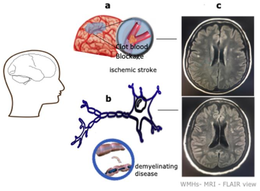
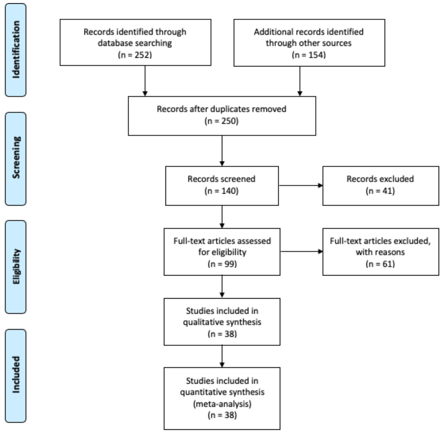
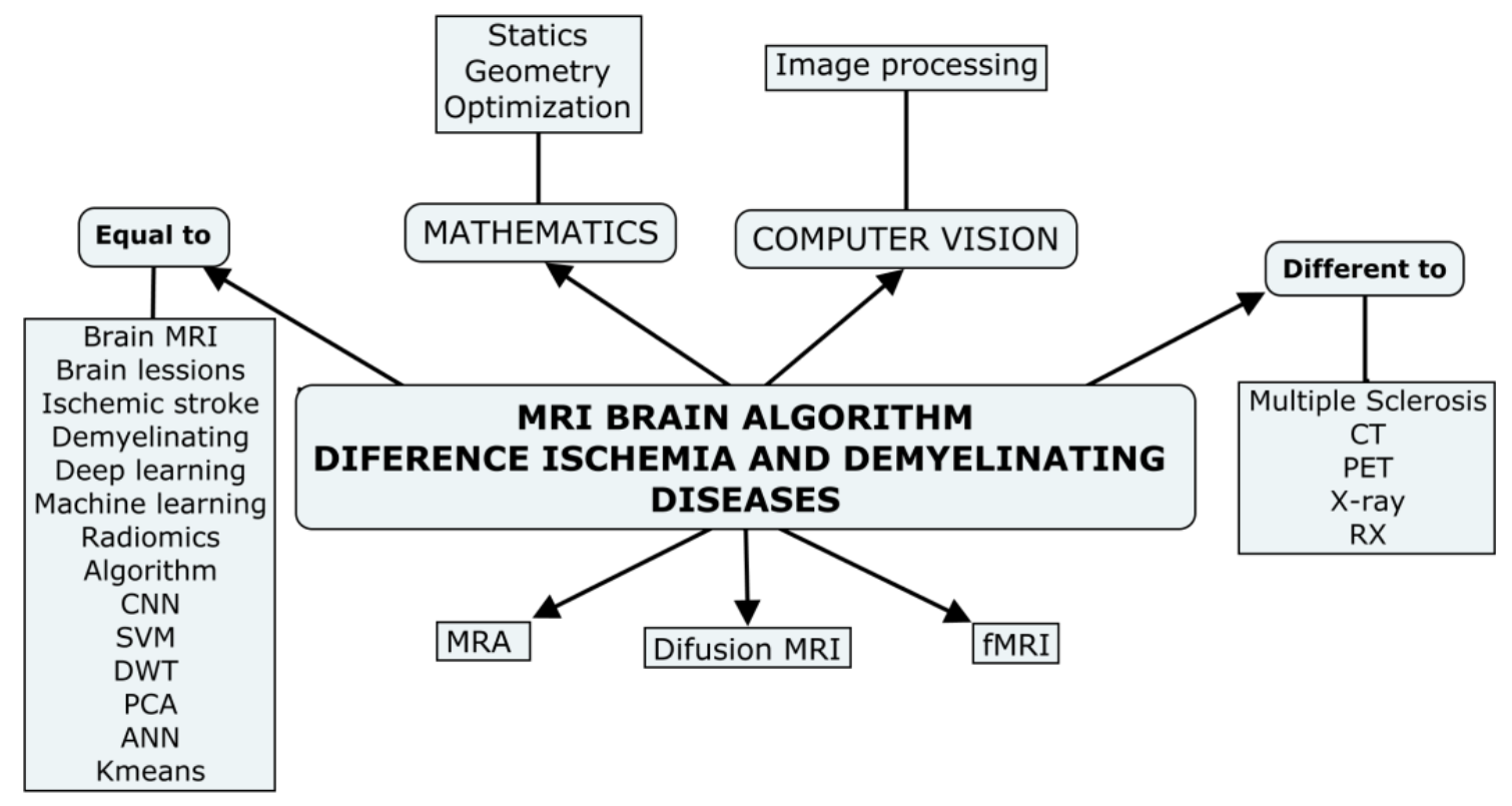
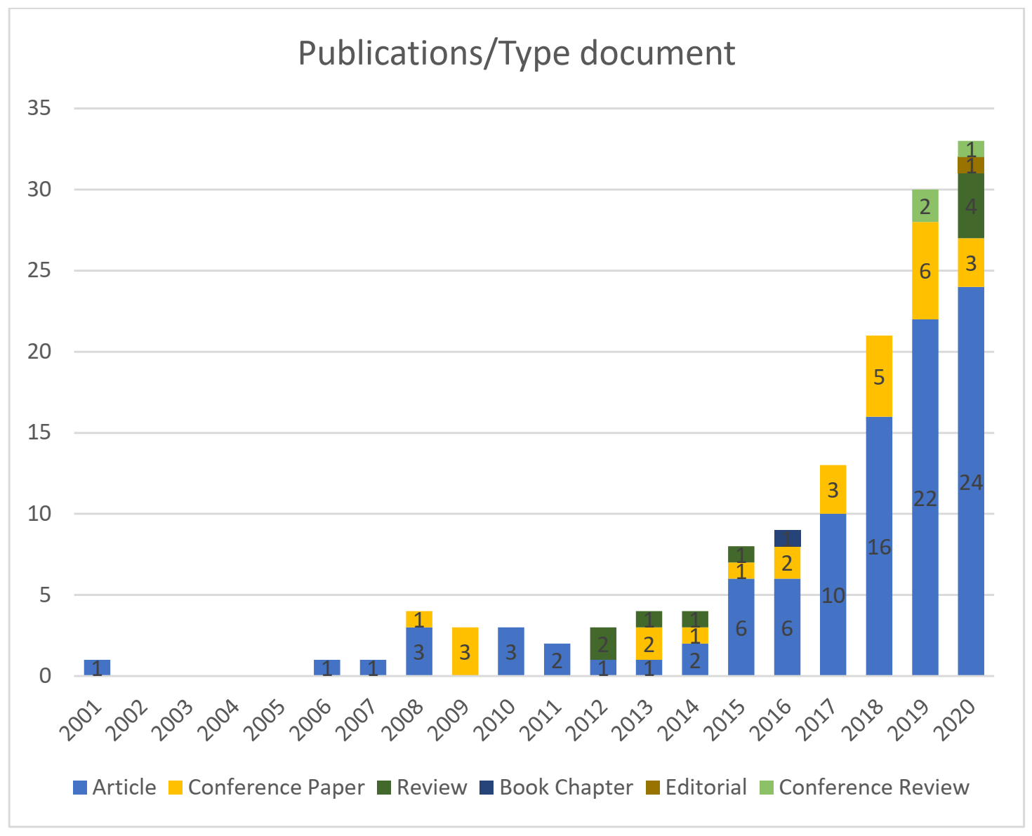
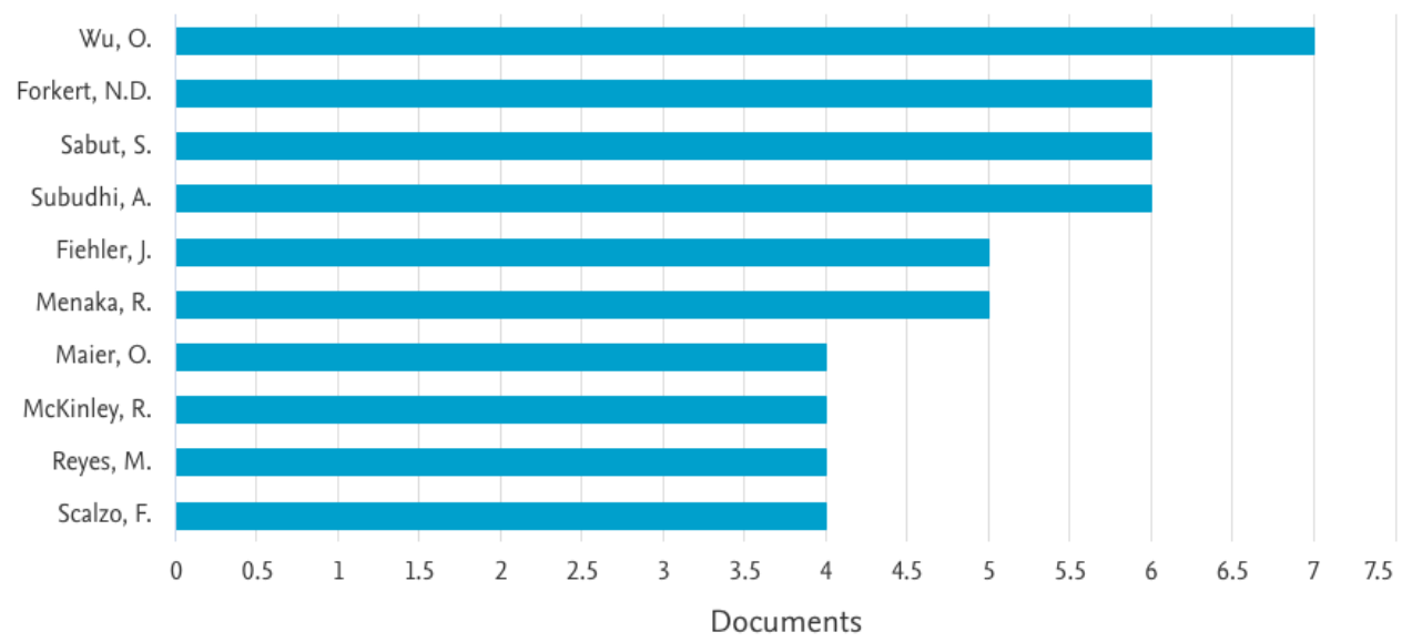
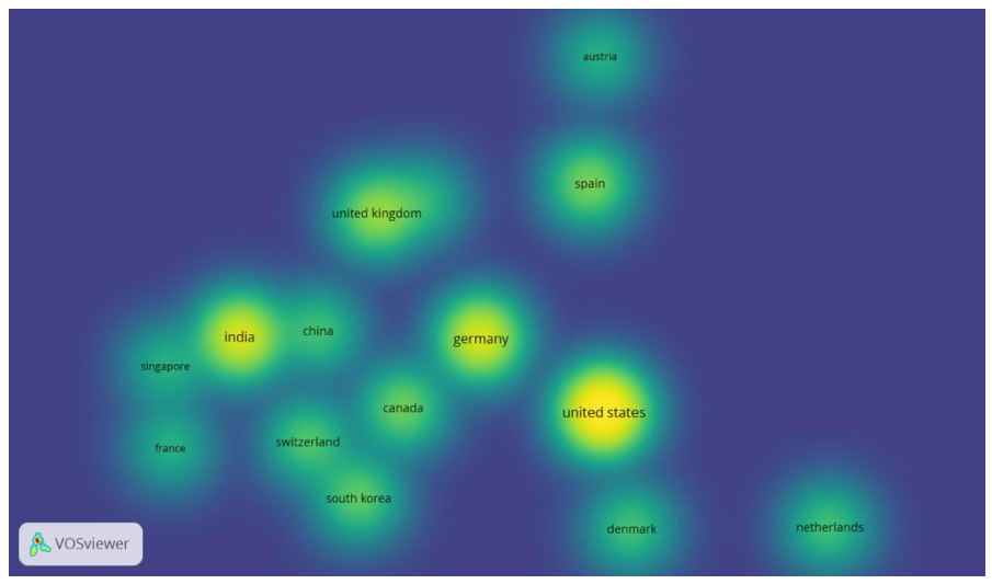
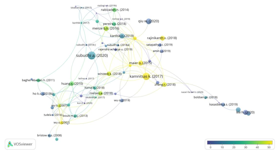
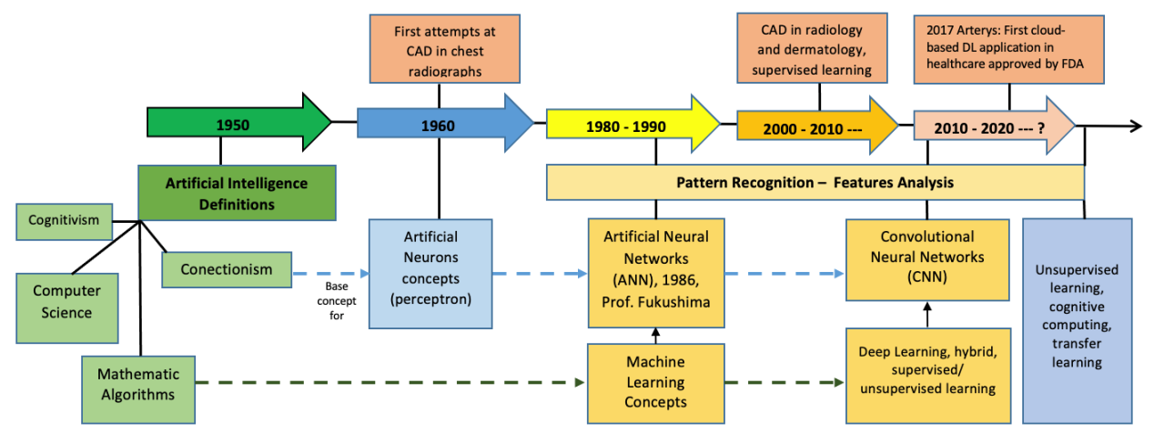
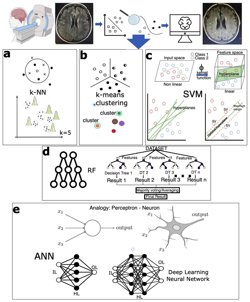
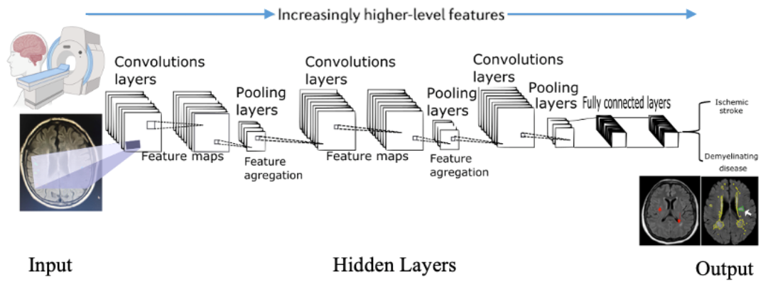
Table 1.
Key words used in the global semantic structure search.
| Magnetic resonance imaging | (((magnetic*) AND (resonanc*) AND (imag* OR picture OR visualiz*)) OR mri OR mra) |
| Brain processing | (algorithm* OR svm OR dwt OR kmeans OR pca OR cnn OR ann)) AND (“deep learning”) OR (“neural networks”) OR (“machine learning”) OR (“convolutional neural network”) OR (“radiomics”) |
| Disease | ((brain* OR cerebrum) AND ((ischemic AND strok*) OR (demyelinating AND (disease OR “brain lesions”)))) |
| Key words for semantic structure search in the Scopus database | TITLE-ABS-KEY ((((magnetic*) AND (resonanc*) AND (imag* OR picture OR visualiz*)) OR mri OR mra) AND ((brain* OR cerebrum) AND ((ischemic AND strok*) OR (demyelinating AND (disease OR “brain lesions”)))) AND (algorithm* OR svm OR dwt OR kmeans OR pca OR cnn OR ann)) AND (“deep learning”) OR (“neural networks”) OR (“machine learning”) OR (“convolutional neural network”) OR (“radiomics”) |
The symbol (*) represents a wildcard to help in the search when a word has multiple spelling variations.
Table 2.
List of the 10 most cited articles according to the normalization of the citations [58]. This table also shows the central theme of research, the type of image, and the methodology used in the processing.
Table 2.
List of the 10 most cited articles according to the normalization of the citations [58]. This table also shows the central theme of research, the type of image, and the methodology used in the processing.
| Article Title | Author/Year | Journal | Total Citations | Norm. Citations | Disease | Type of Images/ Dataset | Methodology | Metrics/ Observation |
|---|---|---|---|---|---|---|---|---|
| Efficient Multi-scale 3D CNN with Fully Connected CRF for Accurate Brain Lesion Segmentation [76] | Kamnitsas, K. et al. (2017) | Medical Image Analysis | 1062 | 7.54 | Brain injuries, brain tumors, ischemic stroke | MRI BRATS 2015 ISLES 2015 | 11-layer-deep 3D CNN | BRATS 2015 DSC: 84.9 Precision: 85.3 Sensitivity: 87.7 ISLES 2015 DSC: 66 Precision: 77 Sensitivity: 63 ASSD: 5.00 Haussdorf: 55.93 |
| ISLES 2015—A Public Evaluation Benchmark for Ischemic Stroke Lesion Segmentation from Multispectral MRI [26] | Maier O. et al. (2017) | Medical Image Analysis | 171 | 1.21 | Ischemic stroke | MR-DWI-PWI | RF-CNN | It is a comparison of tools developed in Challenge ISLES 2015. |
| Classifiers for Ischemic Stroke Lesion Segmentation: A Comparison Study [38] | Maier O. et al. (2015) | PLoS ONE | 78 | 2.87 | Ischemic stroke | MRI—private37 cases (patients) | Generalized linear models RDF CNN | DSC [0, 1]: 0.80 HD (mm): 15.79 ASSD (mm): 2.03 Prec. [0, 1]: 0.73 Rec. [0, 1]: 0.911 |
| Fully Automatic acute Ischemic Lesion Segmentation in DWI Using Convolutional Neural Networks [42] | Chen l. et al. (2017) | NeuroImage: Clinical Smart Innovation, Systems and Technologies, Vol 105. Springer | 77 | 0.55 | Ischemic stroke | MR-DWI—741 private subjects | CNN DeconvNets: EDD Net MUSCLE Net | DSC: 0.67 Lesion detection rate: 0.94 |
| Segmentation of Ischemic Stroke Lesion in Brain MRI Based on Social Group Optimization and Fuzzy-Tsallis Entropy [77] | Rajinikanth, V., Satapathy, S.C. (2018) | Arabian Journal for Science and Engineering | 56 | 2.60 | Ischemic stroke | ISLES 2015 MRI-FLAIR-DWI | Social group optimization monitored Fuzzy-Tsallis entropy | Precision: 98.11% DC: 88.54% Sensitivity: 99.65% Accuracy: 91.17% Specificity: 78.05% |
| Automatic Segmentation of Acute Ischemic Stroke from DWI Using 3-D Fully Convolutional DenseNets [74] | Zhang R. et al. (2018) | IEEE Transactions on Medical Imaging | 47 | 2.18 | Ischemic stroke | MR-DWI—242 private subjects: training (90), testing (90),validation (62) Additional dataset: ISLES 2015-SSIS | 3D-CNN | DSC: 79.13% Lesionwise precision: 92.67% Lesionwise F1 score: 89.25% |
| ISLES 2016 and 2017—Benchmarking Ischemic Stroke Lesion Outcome Prediction Based on Multispectral MRI [75] | Winzeck S. et al. (2018) | Frontiers in Neurology | 45 | 2.09 | Ischemic stroke | MR-DWI-PWIISLES 2016–2017 | RF-CNN | It is a comparison of tools developed in Challenge ISLES 2016–2017. |
| Prediction of Tissue Outcome and Assessment of Treatment Effect in Acute Ischemic Stroke Using Deep Learning [78] | Nielsen, A. et al. (2018) | Stroke | 42 | 1.95 | Ischemic stroke | MRI—222 private cases (patients) | CNN deep | AUC = 0.88 ± 0.12 |
| Enhancing Interpretability of Automatically Extracted Machine Learning Features: Application to a RBM-Random Forest System on Brain Lesion Segmentation [79] | Pereira, S. et al. (2018) | Medical Image Analysis | 30 | 1.39 | Brain lesions: Brain tumor ischemic stroke | MRI—multimodality BRATS 2013: training (30), leaderboard (25), challenge (10) SPES from MICCAI—ISLES: 30 training, 20 challenge | Restricted Boltzmann Machine for unsupervised feature learning, and a random forest classifier | BRATS 2013 Dice score: 0.81 SPES Dice score: 0.75 ± 0.14 ASSD: 2.43 ± 1.93 |
| Predicting Final Extent of Ischemic Infarction Using Artificial Neural Network Analysis of Multi-Parametric MRI in Patients with Stroke [80] | Bagher-Ebadian, H. et al. (2011) | PLoS ONE | 30 | 1.18 | Ischemic stroke | MRI-DWI: 12 subjects | ANN | Map of prediction correlation (r = 0.80, p < 0.0001) |
MRI: magnetic resonance imaging; DWI: diffusion-weighted imaging; PWI: perfusion-weighted imaging; FLAIR: fluid attenuated inversion recovery; BRATS: brain tumor image segmentation; ISLES: ischemic stroke lesion segmentation; MICCAI: medical image computing and computer-assisted intervention; SPES: stroke perfusion estimation; ANN: artificial neural network; CNN: convolutional neural network; RF: random forest; RDF: random decision forest; EDD Net: ensemble of two DeconvNets; MUSCLE Net: multi-scale convolutional label evaluation; DSC: Dice score coefficient; ASSD: average symmetric surface distance; HD: Haussdorf distance.
Table 3.
Summary of CNN architectures and principal libraries used to build models of DL. The data for this were collected from [16,127,128].
| Architectures of a CNN | ||
|---|---|---|
| Name | Reference | Details |
| LeNet | Backpropagation Applied to Handwritten Zip Code Recognition [129] | Yann LeCun 1990. Read zip codes, digits. |
| AlexNet | ImageNet Classification with Deep Convolutional [130] Neural Networks | Alex Krizhevsky, Ilya Sutskever and Geoff Hinton, in 2012 ILSVRC challenge. Similar to LeNet but deeper, bigger, and featured convolutional networks. |
| ZF Net | Visualizing and Understanding Convolutional Networks [131] | Matthew Zeiler and Rob Fergus, ILSVRC, 2013. Expanding the size of the middle convolutional layers and making the stride and filter size on the first layer smaller. |
| GoogLeNet | Going Deeper with Convolutions [132] | Szegedy et al., from Google, ILSVRC 2014. Going Deeper with Convolutions |
| VGGNet | Very Deep Convolutional Networks for Large-Scale Image Recognition [133] | Karen Simonyan and Andrew Zisserman in ILSVRC 2014. The depth of the network is a critical component for good performance. |
| ResNet | Residual Network [134] | Kaiming He et al., in ILSVRC 2015. It features special skip connections and a heavy use of batch normalization. |
| Highway nets | Highway Networks [135] | The architecture is characterized by the use of gating units that learn to regulate the flow of information through a network. |
| DenseNet | Densely Connected Convolutional Networks [136] | The dense convolutional network (DenseNet) connects each layer to every other layer in a feed-forward fashion. |
| SENets | Squeeze-and-Excitation Networks [137] | Model interdependencies between channels of the relationship of features used in a traditional CNN |
| NASNet | Neural Architecture Search Network [138] | Authors propose to search an architectural building block on a small dataset and then transfer the block to a larger dataset. |
| YOLO | You Only Look Once [139] | A unified model for object detection |
| GANs | Generative Adversarial Networks [120] | Framework for estimating generative models via adversarial nets |
| Siamese nets | Siamese Networks [140] | A Siamese neural network is a class of neural network architectures that contain two or more identical subnetworks. The word identical here means that they have the same configuration with the same parameters and weights. |
| U-Net | U-Net: Convolutional Networks for Biomedical Image Segmentation [141] | The architecture consists of a contracting path to capture context and a symmetric expanding path that enables precise localization. |
| V-net | V-Net: Fully Convolutional Neural Networks for Volumetric Medical Image Segmentation [142] | Architecture for 3D image segmentation based on a volumetric, fully convolutional neural network |
| Libraries Used to Build DL Models | ||
| GIMIAS | http://www.gimias.org/ (accessed on 10 December 2020) | A workflow-oriented environment for solving advanced, biomedical image computing and individualized simulation problems |
| SPM | https://www.fil.ion.ucl.ac.uk/spm/ (accessed on 10 December 2020) | The analysis of brain imaging data sequences using statistical parametric mapping as an assessment of spatially extended statistical processes used to test hypotheses about functional imaging data |
| FSL | https://fsl.fmrib.ox.ac.uk (accessed on 10 December 2020) | A collection of analysis tools for functional magnetic resonance images (fMRI), MRI, and diffusion tensor imaging (DTI) brain imaging data |
| PyBrain | http://pybrain.org/ (accessed on 10 December 2020) | Reinforcement learning, artificial intelligence, and neural network library |
| Caffe | http://caffe.berkeleyvision.org/ (accessed on 10 December 2020) | A deep ML framework |
| PyMVPA | http://www.pymvpa.org/ (accessed on 10 December 2020) | Statistical learning analysis platform |
| Weka | https://www.cs.waikato.ac.nz/ml/weka/ (accessed on 10 December 2020) | Data mining platform |
| Shogun | http://www.shogun-toolbox.org/ (accessed on 10 December 2020) | Machine learning framework |
| SciKit Learn | http://scikit-learn.org (accessed on 10 December 2020) | Scientific computation libraries |
| PRoNTo | http://www.mlnl.cs.ucl.ac.uk/pronto/ (accessed on 10 December 2020) | Machine learning framework |
| Tensorflow | http://playground.tensorflow.org (accessed on 10 December 2020) | Created by Google. It provides excellent performance and multiple Central processing units (CPU) and graphics processing unit(GPU) support. |
| Theano | https://pypi.org/project/Theano/ (accessed on 10 December 2020) | Easy to build a network but challenging to create a full solution. Uses symbolic logic and written in Python. |
| Keras | https://keras.io (accessed on 10 December 2020) | Created in Python, it is possible to use with Theano or Tensorflow backend. |
| Torch | http://torch.ch/docs/tutorials-demos.html (accessed on 10 December 2020) | Created in C. Performance is very good. |
| Pytorch | https://pytorch.org (accessed on 10 December 2020) | It is a Python front end to the Torch computational engine. It is an integration of Python with the Torch engine. Performance is higher than Torch with GPU integration facility. |
Table 4.
Summary of datasets dedicated to ischemia (stroke) and demyelinating diseases (multiple sclerosis (MS)). Brain medical image datasets are also listed.
Table 4.
Summary of datasets dedicated to ischemia (stroke) and demyelinating diseases (multiple sclerosis (MS)). Brain medical image datasets are also listed.
| Dataset Name | Details | Type: Private Public | Website | Reference/ Support |
|---|---|---|---|---|
| MICCAI | MS lesion segmentation challenge: data for competition in order to compare algorithms to segment the MS lesions since 2008 | Public and private.Some data require subscription. | https://www.nitrc.org/projects/msseg/ (accessed on 10 December 2020) | Akkus et al. (2017) [9] |
| BRATS | Brain tumor segmentation: MRI dataset for challenge BRATS since 2012.MRI modalities: T1, T1C, T2, FLAIR. BRATS 2015 contains 220 brains with high-grade and 54 brains with low-grade gliomas for training and 53 brains with mixed high- and low-grade gliomas for testing. | Public | https://ipp.cbica.upenn.edu/ (accessed on 10 December 2020) | Menze et al. (2015) [169] |
| ISLES | Dataset used for ischemic stroke lesion segmentation challenge since 2015 in order to evaluate stroke lesion/clinical outcome prediction from acute MRI scans. ISLES has two categories with individual datasets: SISS: sub-acute ischemic stroke lesion segmentation, which contains 36 subjects with modalities FLAIR, DWI, T2 TSE (turbo spin echo), and T1 TFE (turbo field echo). SPES: acute stroke outcome/penumbra estimation, which contain 20 subjects with 7 modalities, namely cerebral blood flow (CBF), cerebral blood volume (CBV), DWI, T1c, T2, Tmax, and time to peak (TTP). | Public, require registration and approval | https://www.smir.ch/ISLES/Start2016 (accessed on 10 December 2020) | Maier et al. (2017) [26] Winzeck et al. (2018) [75] |
| MTOP | Mild traumatic brain injury outcome: MRI data for challenge: 27 subjects | Public | https://www.smir.ch/MTOP/Start2016 (accessed on 10 December 2020) | Akkus et al. (2017) [9] |
| MSSEG | MS data for evaluate basic and advanced segmentation methods; 53 datasets (15 training data and 38 testing data). Modalities: 3D FLAIR, 3D T1-w3D, T1-w Gadolinium, and 2D DP/T2 | Public | https://portal.fli-iam.irisa.fr/msseg-challenge/data (accessed on 10 December 2020) | Commowick et al. (2018) [165] |
| NeoBrainS12 | Set includes T1 and T2 MRI of five infants. Challenge is to compare algorithms for segmentation of neonatal brain tissues and measurement of corresponding volumes using T1 and T2 MRI scans of the brain. | Private | https://neobrains12.isi.uu.nl/?page_id=52 (accessed on 10 December 2020) | Isgum et al. (2015) [170] |
| MRBrainS | Challenge for segmenting brain structures in MRI scans | Private and public, require registration and approval | https://mrbrains13.isi.uu.nl/downloads/ (accessed on 10 December 2020) | Mendrik, A.M. et al. (2015) [171] |
| OpenNeuro | An open repository of MRI, MEG, EEG, intracranial electroencephalography (iEEG), and electrocorticography (ECoG) datasets | Public | https://openneuro.org/ (accessed on 10 December 2020) | Laura and John Arnold Foundation (ljaf) National Science Foundation (NSF) National Institute of Health (NIH) Stanford SquishyMedia |
| UK Biobank | International platform of health data resources. Contain MR images from 15,000 participants, aiming to reach 100,000. | Private— Public, require registration and approval | https://www.ukbiobank.ac.uk/ (accessed on 10 December 2020) | UK Biobank |
| ATLAS | Anatomical Tracings of Lesions After Stroke (ATLAS) is an open-source dataset of 304 T1-weighted MRI with manually segmented lesions and metadata. | Public, require registration and approval | https://www.icpsr.umich.edu/web/pages/ (accessed on 10 December 2020) | Liew et al. [164] |
| ADNI | Alzheimer’s Disease Neuroimaging Initiative contains data from different types (clinical, genetic, MR images, PET images, bioespecimen) | Public, require registration and approval | http://adni.loni.usc.edu/data-samples/data-types/ (accessed on 10 December 2020) | Alzheimers Disease Neuroimaging Initiative (ADNI) |
| ABIDE | Neuroimaging data from the Autism Brain Imaging Data Exchange (ABIDE): 112 datasets from 539 individuals suffering from Autism spectrum disorders (ASD) and 573 typical controls. | Public, require registration and approval | http://preprocessed-connectomes-project.org/abide/ (accessed on 10 December 2020) | Craddock, C. et al. (2013) [172] |
| NIF | Neuroscience information framework project: is a semantically-enhanced search engine of neuroscience information. Data and biomedical resources. | Public | https://neuinfo.org/ (accessed on 10 December 2020) | Neuroscience Information Framework (NIF) |
| NEUROVAULT | A public repository of unthresholded statistical maps, parcellations, and atlases of the brain | Public | https://neurovault.org (accessed on 10 December 2020) | Gorgolewski et al. (2016) [173] |
| Integrated Datasets | A virtual database currently indexing a variety of datasets | Public, require registration | https://scicrunch.org/scicrunch/Resources/record/nlx_144509-1/SCR_010503/resolver (accessed on 10 December 2020) | FAIR Data Informatics Lab University of California, San Diego, USA |
| TCIA | The Cancer Imaging Archive is a repository with different collections of imaging datasets and diseases. | Public, require registration | https://www.cancerimagingarchive.net/collections/ (accessed on 10 December 2020) | Department of Biomedical Informatics at the University of Arkansas for Medical Sciences, USA |
| NiftyNEt | An open source convolutional neural network platform for medical image analysis and image-guided therapy | Public | https://niftynet.io (accessed on 10 December 2020) | Gibson et al. (2018) [174] |
| MONAI | MONAI is a PyTorch-based framework for deep learning in healthcare imaging. It provides domain-optimized foundational capabilities for developing healthcare imaging training workflows in a native PyTorch paradigm. | Public | https://monai.io/ (accessed on 10 December 2020) | Project started by NVIDIA and King’s College London for the AI research community |
| MSD | Medical Segmentation Decathlon: A challenge of machine learning algorithms for segmentation task. Give a data for 10 tasks: brain tumor, cardiac, liver, hippocampus, prostate, lung, pancreas, hepatic vessel, spleen, colon. Modality: MRI and CT | Public | http://medicaldecathlon.com (accessed on 10 December 2020) | Simpson et al. (2019) [175] |
| Grand Challenge | A platform for end-to-end development of machine learning solutions in biomedical imaging | Public: require registration | https://grand-challenge.org/ (accessed on 10 December 2020) | Contributors: Bram van Ginneken, Sjoerd Kerkstra, and James MeakinRadboud University Medical Center in Nijmegen, the Netherlands |
| StudierFenster | Open science platform for medical image processing | Public | http://studierfenster.icg.tugraz.at (accessed on 10 December 2020) | TU and the MedUni Graz in Austria |
Table 5.
Summary of documents related to ischemic stroke and demyelinating disease.
| Author/ Year | Dataset | MRI Technique | Software/ Methods Features Processing | Research Task | Technique AI | Metrics | ||
|---|---|---|---|---|---|---|---|---|
| Type Access | Image Modality | Composition | ||||||
| Huang et al. (2011) [72] | Private: 36 subjects’ experiment (rats), three groups of 12 | MRI: T2 + MRI-CBF-ADC | Method 1 Training: 1 Testing: 11 Method 2 Training: 11 Testing: 1 | Stroke | SVM + ANN | ADC + CBF: 86 + −2.7% 89 + −1.4% 93 + −0.8% | ||
| Giese et al. (2020) | MRI–genetics interface exploration (MRI-GENIE) | MRI: FLAIR | 2529 patients’ scan | Stroke | DL | |||
| Wu et al. (2019) [66] | MRI–genetics interface exploration (MRI-GENIE) | 2770 patients’ scan | Stroke | 3D CNN | Dice score: 0.81–0.96 | |||
| Nazari-Farsani et al. (2020) [33] | Private: 192, 3D MR images | MRI: DWI and ADC | 106 Stroke 86: healthy cases | Stroke | SVM: linear kernel and cross-validation | Accuracy: 73% Precision: 77% Sensitivity: 84% Specificity: 69% | ||
| Anbumozhi (2020) [21] | ISLES 2017: 75 images | MRI | 52: Healthy 23: stroke | Stroke | SVM and k-means clustering | Accuracy: 99.8% Precision: 97.3% Sensitivity: 98.8% Specificity: 94% | ||
| Subudhi et al. (2020) [28] | Private: 192 MR images | MRI: DWI | 122 PACS 36 LACS, 34 TACS | Expectation-maximization (EM) algorithm FODPSO: an advanced optimization method of Darwinian PSO | Stroke: LACS, PACS, TACS | SVM and random forest (RF) | Accuracy: 93.4% DSC: 0.94 | |
| Qiu et al. (2020) [184] | Private: 1000 patients | MRI and CT | Manually defined featuresU-net transfer learning | Stroke | Random forest | Accuracy: 95% | ||
| Li et al. (2004) [185] | Private: 20 patients | Diffusion tensor MRI (DT MRI) | 20 patients | Manual lesion tracing | Stroke | MSSC + PVVR | Similarity: 0.97 | |
| Ortiz-Ramón et al. (2019) [186] | Private: 100 patients | MRI: T1-weighted, T2-weighted, FLAIR | 20 patients | 1.5T GE Signa LX clinical scanner (General Electric, Milwaukee, WI | Software FSL, 3D texture analysis | Stroke | SVM (linear kernel) + random forest | AUC: 0.7–0.83 |
| Raina et al. (2020) [187] | ISLES 2015 | FLAIR, DWI, T1, T1-contrast | 28 patients | Reflective registration: free registration image with a reflected version of itself. FSL | Stroke | Two-path CNN + NLSymm Wider2dSeg + NLSymm | DSC: 0.54; 0.62 Precision: 0.52; 0.68 Recall: 0.65; 0.60 | |
| Grosser et al. (2020) [188] | Private: 99 patients | MRI: DWI and PWI, FLAIR | 99 patients | Software AnToNIa: tool for analysis multipurpose MR perfusion datasets | Stroke | ML: logistic regression, random forest, and XGBoost | ROC AUC: 0.893 +/−0.085 | |
| Lee et al. (2020) [189] | Private: 355 patients | MRI: DWI-FLAIR | 355 patients: 299 to train; 56 to test | 89 vector features | Stroke | ML: logistic regression, random forest, and SVM | Sensitivity and Specificity; Logistic Regression: 75.8%, 82.6% SVM: 72.7%, 82.6%. Random Forest: 75.8%,82.6% | |
| Melingi y Vivekanand (2018) [167] | Private, real-time dataset | MRI-DWI | Ischemic stroke | Kernelized fuzzy C-means (KFCM) clustering and SVM | Accuracy: 98.8% Sensitivity: 99% | |||
| Clêrigues et al. (2020) [190] | ISLES 2015 | Multimodal MRIT1, T2, FLAIR, DWI | Sub-acute ischemic stroke segmentation (SISS): 28 training and 36 testing cases Stroke penumbra estimation sub-task (SPES): 30 training and 20 testing cases | SISS and SPES | U-Net based CNN architecture using 3D convolutions, 4 resolution steps and 32 base filters | SISS: DSC = 0.59 ± 0.31 SPES: DSC = 0.84 ± 0.10 | ||
| Kumar et al. (2020) [179] | ISLES 2015 ISLES 2017 | Multimodal MRI: T1, T2, FLAIR, DWI | ISLES 2015 (SISS): 28 training and 36 testing cases (SPES): 30 training and 20 testing cases ISLES 2017: 43 training and 32 test cases | Ischemic stroke | Classifier-segmenter network:a combination of U-Net and fractal networks | ISLES 2015 (SISS) Accuracy: 0.9914 Dice coeff: 0.8833 Recall: 0.8973 Precision: 0.8760 ISLES 2015-SPES Accuracy: 0.9908 Dice coeff: 0.8993 Recall: 0.9091 Precision: 0.9084 ISLES 2017 Accuracy: 0.9923 Dice coeff: 0.6068 Recall: 0.6611 Precision: 0.6141 | ||
| Leite et al. (2015) [20] | Private images from 77 patients | T2-weighted MRI | 50 with MS, 19 healthy, 4 stroke 75% training set 25% testing set | WMH Stroke MS | Classifiers: SVM with RBF kernel OPF: optimum path forest with decision tree, LDA: Linear discriminant analysis with PCA kNN: k-nearest neighbor, K = 1, K = 3, K = 5 | Accuracy for classifier demyelinating and ischemic SVM: 86.5 +/− 0.09 k-NN: 83.57 0.07 OPF:81.23 0.06 LDA: 83.52 0.06 | ||
| Ghafoorian et al. (2016) [19] | Private: 362 patients’ MRI scans | FLAIR | 312 Training 50 Testing | WM cerebral SVD | AdaBoost + random forest | FROC analysis Sensitivity: 0.73 with 28 false positives | ||
| Bowles et al. (2017) [180] | Private Brain Research Imaging Centre of Edinburgh, 127 subjects | FLAIR | 20 Training | GE Signa Horizon HDx 1.5 T clinical scanner | Cerebral SVD MS | Image synthesis Gaussian mixture models SVM All of them compared with publicly available methods LST LesionTOADS and LPA | DSC: 0.70 ASSD: 1.23 HD: 38.6 Prec: 0.763 Recall: 0.695 Fazekas correlation: 0.862 ICC: 0.985 | |
| Brosch et al. (2016) [191] | MICCAI 2008 ISBI 2015 Private, clinical: 377 subjects | T1, T2, PD, and FLAIR T1, T2, PD, and FLAIR T1, T2, and FLAIR | MICCAI Training: 20 Testing: 23 ISBI Training: 20 Testing: 61 Validation: 1 CLINICAL: Training: 250 Testing: 77 Validation: 50 | Private: 1.5T and 3T scanners | MS | 3D Convolutional encoder networks | MICCAI VD: UNC 63.5%, CHB 52.0% TPR: UNC 47.1%, CHB 56.0% FPR: UNC 52.7%, CHB 49.8% ISBI DSC: 68.3% LTPR: 78.3% LFPR: 64.5% CLINICAL: DSC: 63.8% LTPR: 62.5% LFPR: 36.2% VD: 32.9 | |
| Valverde et al. (2017) [192] | (a) MICCAI 2008 (b) Private, clinical 1: 35 subjects (c) Private, clinical 2: 25 subjects | (a) T1, T2, PD, and FLAIR (b) T1, T2 and FLAI,R (c) T1, T2, and FLAIR | (a) Training:20 Testing: 25 (b) Training: ... Testing: ... (a) Training: ...Testing: ... | MS | 3D Cascade CNN | (a) VD: UNC 62.5%, CHB 48.8% TPR: UNC 55.5%, CHB 68.7% FPR: UNC 46.8%, CHB 46.0% (b) DSC: 53.5% VD:30.8% TPR: 77.0% FPR: 30.5% PPV: 70.3% (c): DSC: 56.0% VD: 27.5% TPR: 68.2% FPR: 33.6% PPV: 66.1% | ||
| Praveen et al. (2018) [193] | ISLES 2015: 28 volumetric brains | T1, FLAIR, DWI, and T2 | Training: 27 Testing: 1 | Ischemic stroke | Stacked sparse autoencoder (SSAE) + SVM | Precision: 0.968 DC: 0.943 Recall: 0.924 Accuracy: 0.904 | ||
| Guerrero et al. (2018) [125] | Private Brain Research Imaging Centre of Edinburgh, 127 subjects | T1 and FLAIR | Training: 127 | GE Signa Horizon HDx 1.5 T clinical scanner (General Electric, Milwaukee, WI) | WMH stroke | CNN—u-shaped residual network (uResNet) architecture | WMH Dice (std): 69.5 (16.1) Stroke Dice (std): 40.0 (25.2) | |
| Mitra et al. (2014) [182] | Private: 36 patients | T1W, T2W, FLAIR, and DWI | 3T MR (Magneton Trio; Siemens, Erlangen, Germany) scanner | Lesion (WMH) Ischemic stroke MS | Random forest | DSC (std): 0.60 (0.12) PPV (std): 0.75 (0.18) TPR (std): 0.53 (0.13) SMAD (std): 3.06 (3.17) VD (%) (std): 32.32 (21.64) | ||
| Menze et al. (2016) [36] | BRATS 2012–2013 Glioma data Private dataset for Stroke(Zurich): 18 datasets | T1, T2, T1W and FLAIR | Glioma Ischemic stroke | Gaussian mixtures and a probabilistic tissue atlas that employs expectation-maximization (EM) segmenter | FLAIR BRATS glioma, DSC: 0.79 (±0.06) Zurich Stroke DSC: 0.79 (±0.07) T1cBRATS glioma, DSC: 0.66 (±0.14) Zurich stroke DSC: 0.6479 (±0.18) | |||
| Subudhi et al. (2018) [194] | Private:142 patients | MR DWI | GE Medical Systems MRI 1.5 T and flip angle of 55° | Ischemic stroke | Watershed, relative fuzzy connectedness, and guided filter + multilayer perceptron (MLP) and RF | MLP NN DSC: 0.86 Random Forest DSC: 0.95 | ||
| Karthik et al. (2019) [168] | ISLES 2015: 28 volumetric brains | Multimodal MRI T1,T2,FLAIR, DWI | Ischemic stroke | FCN, propose variant of U-Net architecture CNN | DSC: 0.70 | |||
| Boldsen et al. (2018) [195] | Private: 108 patients | MRI: DWI | GE Signa Excite 1.5 T, GE Signa Excite 3 T, GE Signa HDx 1.5 T, GE Signa Horizon 1.5 T, Milwaukee, WI; Siemens TrioTim 3 T, Siemens Avanto 1.5 T, Siemens Sonata 1.5 T, Germany; Philips Gyroscan NT 1.5 T, Phillips Achieva 1.5 T, and Philips Intera 1.5 T, the Netherlands | Ischemic stroke | ATLAS machine learning algorithm COMBAT stroke | ATLAS Dice score: 0.6122 COMBAT stroke Dice score: 0.5636 | ||
| Wottschel et al. (2019) [196] | Private: 400 patients multicentre | T1, T2-weighted MRI | MS-WM lesions | SVM with cross-validation | Accuracy for multicentre (all dataset): 64.8–70.8% Accuracy for individual center (small dataset) 64.9–92.9% | |||
CBF: cerebral blood flow; ADC: apparent diffusion coefficient; SVD: small-vessel disease; TACS: total anterior circulation stroke syndrome; PACS: partial anterior circulation stroke syndrome; LACS: lacunar stroke syndrome; SISS: sub-acute ischemic stroke segmentation; SPES: stroke penumbra estimation; FROC: free-response receiving operating characteristic; COMBAT Stroke: computer-based decision support system for Thrombolysis in stroke.
Publisher’s Note: MDPI stays neutral with regard to jurisdictional claims in published maps and institutional affiliations. |
© 2021 by the authors. Licensee MDPI, Basel, Switzerland. This article is an open access article distributed under the terms and conditions of the Creative Commons Attribution (CC BY) license (http://creativecommons.org/licenses/by/4.0/).
Share and Cite
MDPI and ACS Style
Castillo, D.; Lakshminarayanan, V.; Rodríguez-Álvarez, M.J. MR Images, Brain Lesions, and Deep Learning. Appl. Sci. 2021, 11, 1675. https://doi.org/10.3390/app11041675
AMA Style
Castillo D, Lakshminarayanan V, Rodríguez-Álvarez MJ. MR Images, Brain Lesions, and Deep Learning. Applied Sciences. 2021; 11(4):1675. https://doi.org/10.3390/app11041675
Chicago/Turabian StyleCastillo, Darwin, Vasudevan Lakshminarayanan, and María José Rodríguez-Álvarez. 2021. "MR Images, Brain Lesions, and Deep Learning" Applied Sciences 11, no. 4: 1675. https://doi.org/10.3390/app11041675
Note that from the first issue of 2016, this journal uses article numbers instead of page numbers. See further details here.