The Usage of the Harmony Search Algorithm for the Optimal Design Problem of Reinforced Concrete Retaining Walls

Abstract

In this paper, the Harmony Search (HS) algorithm is utilized to perform single and multivariate parametric studies to acquire the optimization of both size and cost of reinforced concrete (RC) retaining walls embedded in pure frictional soils. The geotechnical properties of the backfill and foundation soil such as shear strength angle, unit weight, and the ultimate bearing pressure of the soil have been used to create different cases for evaluating the effects of site properties on the size and cost of the wall. The change of depth of excavation and surcharge loading condition is fictionalized for generating different environmental conditions for all envisaged soil profiles to predict possible rates of influences. The unit cost of the concrete has also been evaluated as a variant to show the economic constraints on the selection of structural materials. The results of the analyses represent the integrated influences of different significant parameters on the achievement of minimum cost-dimension optimization. Besides, a well-known commercial geotechnical engineering software is used to compare the appropriateness of the suggested designs in terms of both the attainment of geotechnical stability and the structural requirements. Consequently, this study can guide both researchers and designers to select the proper and optimal sections of RC-retaining wall systems with simultaneous analyses of parameters that are influenced by the design process. Furthermore, the optimization results indicate that a significant cost reduction may be achieved when compared with the traditional pre-design method.

1. Introduction

Reinforced concrete (RC) cantilever retaining walls are frequently used as vertical structural elements constructed to resist the lateral earth pressure by providing stability conditions. The stability term needs to satisfy both geotechnical and structural design requirements due to the interaction between soil and structure. The geotechnical design process of RC cantilever retaining walls involves stability requirements against the possibility of sliding, bearing capacity, and overturning. Studies including the investigations about the geotechnical design of retaining walls began with the development of lateral earth pressure theories proposed by Coulomb [1], Rankine [2], Boussinesq [3], Terzaghi [4], and Jacky [5]. Several studies have been conducted to predict the lateral load distributions due to the soil properties and their effects on the stability analysis performed by limit equilibrium solutions [6,7,8,9,10]. Under the above-mentioned stability purposes, the sections of the RC cantilever retaining walls have to acquire adequate shear and also moment capacities, the ultimate bearing pressure of the foundation soil does not allow the tensile stress, and the steel reinforcement used must satisfy the relevant code requirements for ensuring structural safety. To evaluate structural stability and minimization of flexural moments, a lot of research has been performed. In this context, Rhomberg and Street [11] utilized from the optimization techniques for the first time to obtain an optimal design for a retaining wall, Sarıbaş and Erbatur [12] studied the optimization problem of retaining walls in terms of a nonlinear programming state and focused on the weight optimization of the wall. Sasidhar et al. [13] performed optimum design analyses of retaining walls with the use of genetic algorithm that is concerning a structural synthesis which collects all engineering aspects to develop structures not only safe but also economic. In addition, Ashawi et al. [14] investigated the structural behavior of the tied-back retaining walls with a newly written computer code with a finite element-based software. Keskar and Adidam [15] used the relevant Indian Code of Practice to study the constrained optimization problem of retaining walls in terms of the material cost as the objective function. Dembicki and Chi [16] formulated an optimum design method for retaining walls as a non-linear multi-objective problem to minimize both the total weight and to maximize the structure stability. Pochtman et al. [17] considered the optimal design problem of the retaining walls with anchorage. Chau et al. [18] developed a prototype hybrid knowledge-based system to solve the optimum design problem of liquid retaining structures by an integrated consideration of the blackboard architecture, an expert system shell Visual Rule Studio and genetic algorithm. Sivakumar Babu and Basha [19] developed an approach for reliability-based design optimization of reinforced retaining walls considering the change of the treating backfill and foundation soil properties, geometrical properties of wall, and reinforcement and concrete properties as random variables. As a consequence of conducted studies with both engineering disciplines, the selected dimensions of the retaining wall system have to be supplied with. That is why, in practice, the first step of the design process involves selecting some of the dimensions according to experiential studies. This process is called proportioning or pre-design which allows for trial and error sequence until the sizes are finalized [20]. Pre-design sizes can be found in several studies [20,21,22], research reports [23] and codes [24,25]. The experiential proportioning process only involves ensuring stability requirements, but an expedient design has to develop the structures in both safety and minimum cost. Therefore, evaluating the optimum costs of structures with safe sizing can be defined as the most significant factor of the design stage. Methods for obtaining cost and sizing equilibrium of reinforced concrete retaining walls have been the main objective of many studies over the years and continue to be relevant due to the developments in information and computer technologies. Metaheuristic algorithms such as the genetic algorithm (GA) [12,26,27,28], big bang big crunch (BBBC) [29,30], particle swarm optimization (PSO) [31,32], firefly algorithm (FA) [33,34], harmony search (HS) algorithm [35,36], ant colony optimization (ACO), bat algorithm (BA) [37], charged system search (CSS) [38], simulated annealing (SA) [39,40,41], biogeography-based optimization algorithm (BBO) [42], teaching learning-based optimization (TLBO) [43], jaya algorithm (JA) [44], and flower pollination algorithm (FPA) [45] can be counted as the applied mew methods for the optimization process of retaining wall systems.

In the present study, sizing optimization via cost control process is taken into account for RC cantilever retaining walls with the use of the HS provided with MATLAB software. It is the aim to investigate the effects and influence rates of different soil properties, excavation depths, loading conditions, and material cost change on the dimensional requirements of supporting systems due to the cost optimization. Not only have a huge number of (105,000) analyses been performed to control the optimum dimensions of the wall system, but also evaluations have been made to obtain the relationships between the variants via dimensions and costs. Besides, the geotechnical software Geo5 which is working with the combined logic of both theoretical [46] analytical methods and finite element method [47], has been used to verify the stability conditions for the suggested cross sections by the performance of the optimization process. At last, the original novelty of this study compared with the related literature can be listed as follows:

• The most important parameters that can be effective for both safety and cost have been handled unprecedentedly by using a very wide parameter network for the design of RC-retaining walls.
• Both individual and dual effects of influencer design parameters are investigated.
• Results of the optimization analyses are compared by interpretations against the traditional pre-design method.
• Verification of the suggested solution method is conducted with a well-known geotechnical design software and the practicality of the usage of the HS algorithm is emphasized in terms of geotechnical engineering.

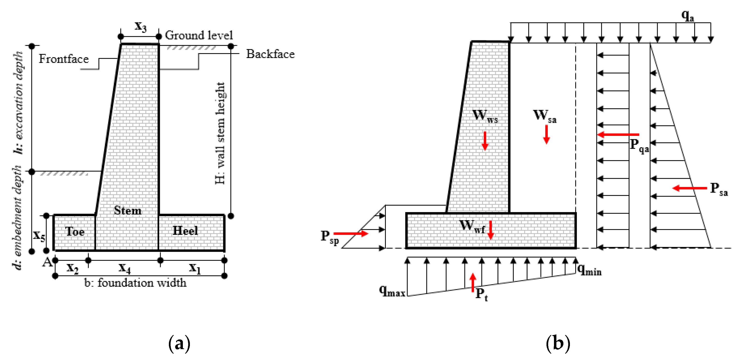
2. Stability Analysis Relating to the Design of RC-Retaining Walls

The profile of a standard T shaped retaining wall is given in Figure 1a. In Figure 1 the height of RC-retaining wall stem, depth of excavation, depth of embedment, the thickness of the wall foundation, the thickness of the wall stem at the top, the thickness of the wall stem at the bottom, the length of the toe, and the length of the heel are abbreviated by H, h, d, x₅, x₃, x₄, x₂, and x₁, respectively.

The mobilized stresses according to the excavation process can be defined as active and passive stress states and the distribution of the mentioned stresses are illustrated in Figure 1b. Generally, RC cantilever retaining walls at the planning stage can be designed for the active soil pressure case when the wall is sufficiently flexible [20]. Keeping this situation in mind, only active pressures are taken into consideration for calculations. Lateral earth pressures are calculated by Rankine Earth Pressure Theory with the use of Equations (1) and (2) for active (K_a) and passive (K_p) states [2].

$$K_a=ta{n}^2(45-\frac{\varnothing }{2})$$

(1)

$$K_p=ta{n}^2(45+\frac{\varnothing }{2})$$

(2)

P_sa and P_sp are the horizontal soil reaction forces for active and passive sides and can be calculated by Equations (3) and (4). The terms γ_s1, K_a1, c_s1, and γ_s2, K_a2, c_s2. γ represents the unit weight of soil, K_a represents active lateral earth pressure coefficient, and c_s represents the cohesion of the soil at the active site and the passive side of the wall, respectively. In Figure 1b and Figure 2b, it is supposed that a surcharge (q_a) is applied to the retaining system from the active side.

$$P_{sa}=\frac{1}{2}{\gamma }_{s1}{H}^2{K}_{a1}-2c_{s1}H\sqrt{K_{a1}}$$

(3)

$$P_{sp}=\frac{1}{2}{\gamma }_{s2}{d}^2{K}_{p2}+2c_{s2}d\sqrt{K_{p2}}$$

(4)

This surcharge is used to determine the acting horizontal load (P_qa) by the use of K_a1. The horizontal value of distributed load (P_qa) that is affected to the wall section from the active site of the wall can be determined by the multiplication of vertical surcharge (q_a) with the height of the wall (H) and with the active lateral earth pressure. W_ws and W_wf represent the weight of the stem and foundation base. W_sa represents the backfill soil weight existing on the foundation base. q_max and q_min values are the base pressures.

The sections of the wall have to be satisfied with both the equilibrium of forces and moment. Unbalanced external and internal loads can make possible modes of failure like sliding, overturning, and/or overstress in soil. The combination of lateral forces can cause the wall to slide through its base. The ratio of the total lateral resisting forces (ΣF_R) to the total lateral sliding forces (ΣF_s) gives the factor of safety value for sliding (Equation (5)). The resisting forces can be combined by the weights of the wall sections, the foundation soil friction resistance, and the lateral components of passive soil forces. Sliding forces include the lateral components of active soil forces and the influence of the loads acting from the backfill side.

$$Fo{S}_s=\frac{\Sigma F_R}{\Sigma F_S}$$

(5)

Another mode of failure consists of the overturning of the wall system about its toe point. The ratio of the total moments of resisting forces (ΣM_R) to total moments of sliding forces (ΣM_S) gives the factor of safety value for overturning (Equation (6)). Resisting moments are generated by the passive pressure of the soil, the self-weight of the overall wall, and the weight of backfill. Overturning moments can be generated by the active pressure of the soil and the surcharge loads which is acting from the active site of the RC wall. “A” point, shown in Figure 1, represents the overturning point of the wall. Sliding and resisting moment values can be calculated by the use of the distances between the envisaged forces and this mentioned point.

$$Fo{S}_o=\frac{\Sigma M_R}{\Sigma M_S}$$

(6)

The third mode of failure is soil bearing capacity failure and it can be evaluated by the ratio of ultimate bearing pressure of the soil (q_z,u) to the maximum degree of soil bearing pressure of the foundation (q_{z, max}) mobilized through the toe of the wall (Equation (7)).

$$Fo{S}_{bc}=\frac{q_{z,u}}{q_{z,max}}$$

(7)

The determination of the maximum and minimum limit values of foundation soil bearing pressure can be made by the use of Equation (8). It has to be noted that this equation is derived for shallow foundations.

$$q_{\begin{array}{c}min\\ max\end{array}}=\frac{\Sigma V}{b}(1\pm \frac{6e}{b})$$

(8)

e is the eccentricity value that can be defined between the moment and total vertical loads [20,48].

$$e=\frac{b}{2}\frac{\Sigma M_R-\Sigma M_0}{\Sigma V}$$

(9)

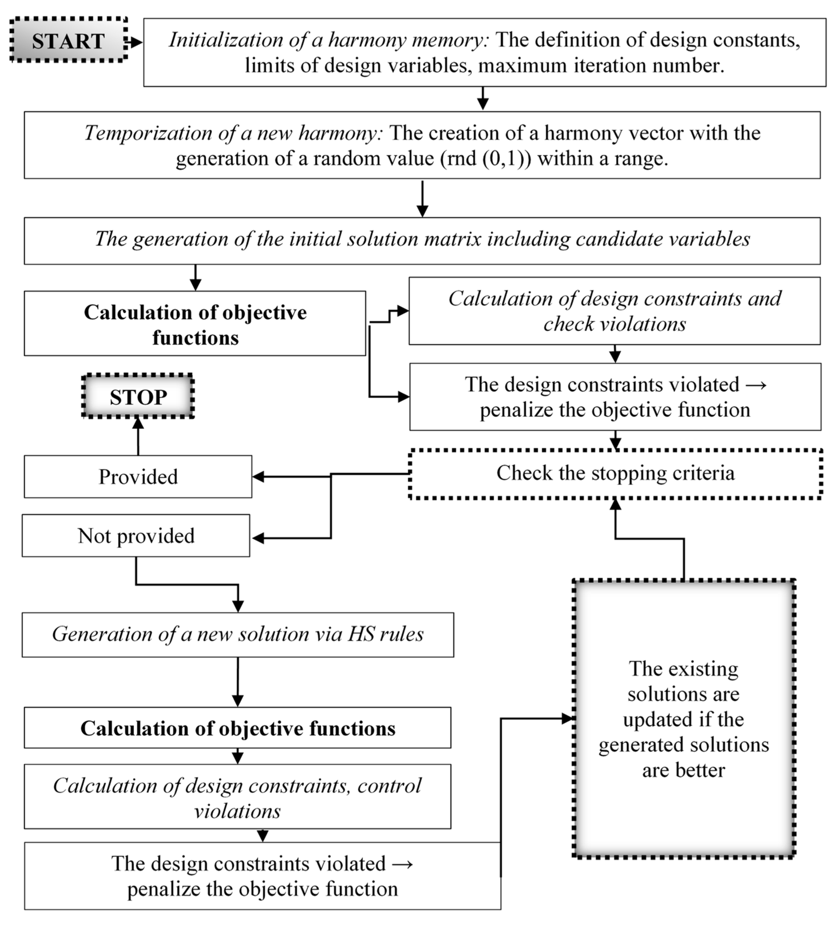
3. Harmony Search (HS)

HS is a meta-heuristic algorithm that is developed by Geem et al. [49]. The logic of the algorithm is depending on the natural musical performance which searches for a perfect state of harmony that is similar to pending jazz improvisation. This situation causes us to achieve a musically pleasing harmony as a perfect state. The perfect state can be calculated by an aesthetic standard and the process of obtaining the optimum solution investigates to find a global solution as a perfect state that is derived by the use of an objective function. The application of HS is based on the specific steps that are given in Figure 2 [50,51,52]. There are three parameters used in HS: harmony memory size (HMS), the pitch adjustment rate (PAR), and the harmony memory consideration rate (HMCR) at the first step of the application process. In general, the application process of the algorithm can be divided into five sequential steps. The first step consists of the definitions of the mentioned specific parameters like design constants, boundary values, and maximum iteration number. New harmony is temporized from the generation of a harmony vector with the presence of a random (rnd (0,1)) value which ranged between 0 and 1. Equation (10) is given to derive the upper (X_i,max) and the lower (X_i,min) limits of each (X_i).

$$X_i=X_{i,min}+rnd(0,1)·(X_{i,max}-X_{i,min})$$

(10)

The mentioned design constants and variables are used to calculate the design equations and then, the result of the objective function can be acquired. The outcomes of this solution are kept in the harmony vector. This process is reproducible depending on the HMS. The whole generated harmony vectors are kept in the initial solution matrix. In the second step, HMCR is utilized to reproduce a new vector by the selection of the appropriate method of solution. In such a case, the calculated HMCR value is bigger than the random one and the first method called general optimization of a vector is chosen by the generation of a random value. If it is not, a local optimization method is chosen. The third stage begins with the creation of a new harmony vector by the start of the iteration process. The specific rules of the HS algorithm are applied to obtain a new harmony vector with the use of different methods. The upper and lower boundaries are utilized as the limits to form the design variables randomly within the first method (Equation (10)). The probability to use a new vector generated with the use of a selected vector from the solution matrix (X_i,old) can be used as the second method to apply. The new values (X_i,new) are derived by adding the multiplication of PAR, the difference of the design variable limits, and rnd (0,1). The mathematical expression of the mentioned relation is given by Equation (11).

$$X_{i,new}=X_{i,old}+rnd(0,1)·PAR ·(X_{i,max}-X_{i,min})$$

(11)

In the fourth stage, comparisons are conducted between the new vector and the stored vectors within the solution matrix. A new vector is selected rather than the existing one provided that the next vector is better than the existing one. If not, the existing situation of the solution matrix is saved. The values that are achieved from the solution of the objective function are compared and the minimum value of the solutions is chosen as the best one. The comparison process is performed with the consideration of the design constraints. Besides, the number of the violations are controlled and the calculation that includes the minimum violation is chosen to be the better one if the violations of the design constraints exist for a new solution and existing solutions. If one of them is violated, the violated solution is eliminated. In the fifth stage, the control of the stopping criterion is done. The stop of the iterations is done if a satisfactory stopping criterion is reached. The maximum iteration number was assumed to be the stopping criterion in this study although there are various ways. Depending on the mentioned clear application process and the succeeding application examples in the literature studies [53,54,55,56,57], the HS algorithm has been chosen to be used in this study as an effective method among metaheuristic algorithms.

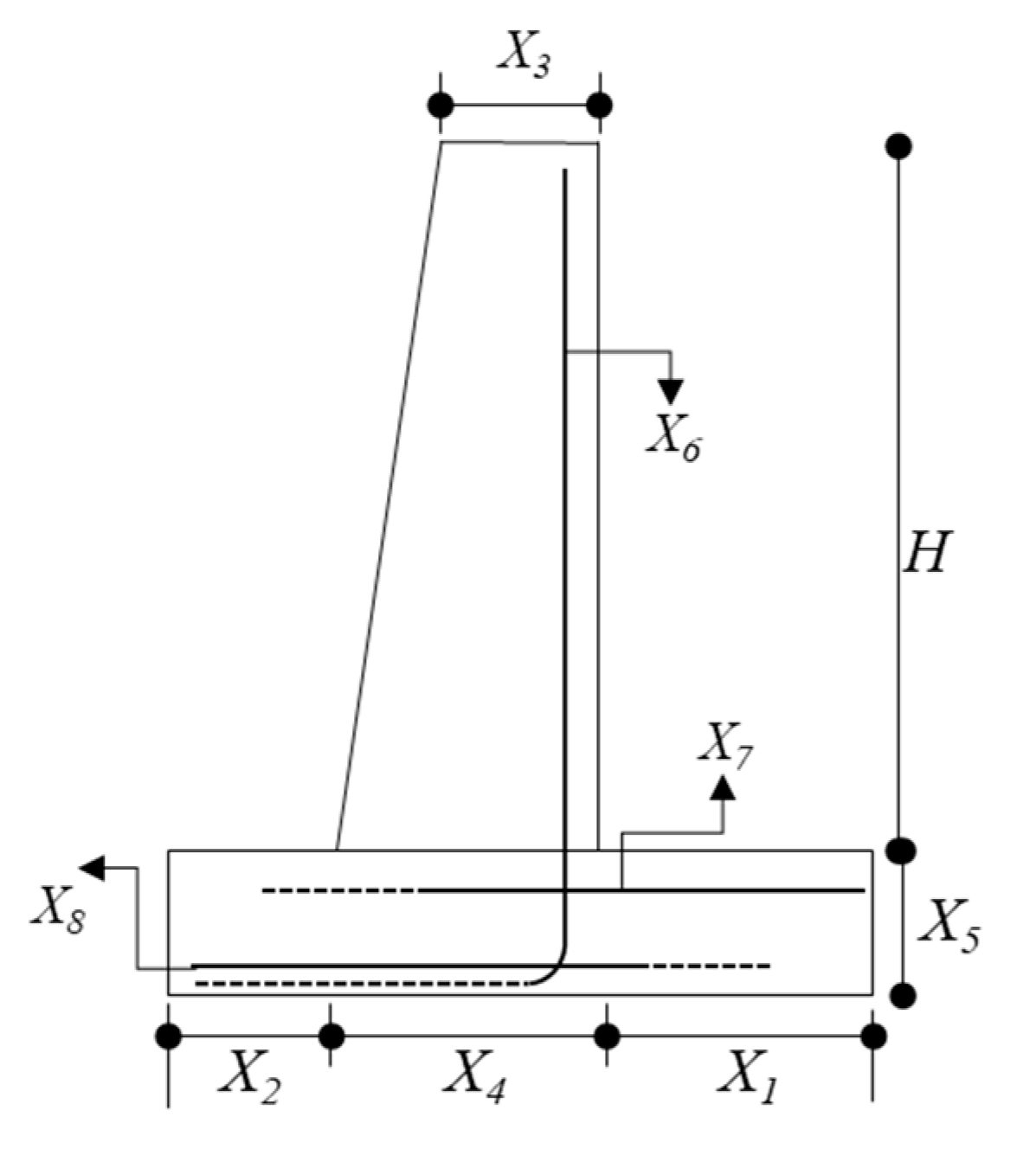
3.1. Design Variables

To apply HS analysis, a special design parameter set is generated for cantilever RC-retaining walls. Totally eight design parameters (X₁, X₂, X₃, X₄, X₅, X₆, X₇, X₈) are defined for cantilever RC-retaining walls in Figure 3. The definitions of related design parameters of cantilever RC-retaining walls are given in

Table 1. Definitions of wall design variables.

	Symbol	Parameter Description
Variables about Cross-section dimension	X1	The length of the wall heel (x1)
	X2	The length of the wall toe (x2)
	X3	The thickness of the wall stem at the top (x3)
	X4	The thickness of the wall stem at the bottom (x4)
	X5	The thickness of the wall foundation (x5)
Variables about reinforced concrete design	X6	Area of reinforcing bars of the stem
	X7	Area of reinforcing bars of foundation heel
	X8	Area of reinforcing bars of the toe

.

3.2. Design Constraints

There are three factors of safety for cantilever RC-retaining wall design. The structural requirement of the wall system is stated depending on American Concrete Institute Building Code Requirements for Structural Concrete (ACI 318-14) [58] by Equation (12). ACI code suggests using the equivalent rectangular compressive stress distribution, so the moment capacity of cantilever RC-retaining walls can be calculated.

$$g_{(j)}(x)\le 0 j=1,m$$

(12)

In Equation (12), m represents the number of design constraints which are defined in

Table 2. The constraints of design on strength and dimensions.

Description	Constraints
Safety condition for overturning stability	g1(X): FoSot,design ≥ FoSot
Safety condition for sliding	g2(X): FoSs,design ≥ FoSs
Safety condition for bearing capacity	g3(X): FoSbc,design ≥ FoSbc
Minimum bearing stress (qmin)	g4(X): qmin ≥ 0
Flexural strength capacities of critical sections (Md)	g5–7(X): Md ≥ Mu
Shear strength capacities of critical sections (Vd)	g8–10(X): Vd ≥ Vu
Minimum reinforcement areas of critical sections (Asmin)	g11–13(X): As ≥ Asmin
Maximum reinforcement areas of critical sections (Asmax)	g14–16(X): As ≤ Asmax

. The inequality of the function belongs to the design variable vector that can be addressed by X_T = {X₁, X₂ …, X_n}. The critical sections that can be defined as the highest moment and shear-force location of the stem and the foundation can only be controlled by the design of the reinforcement.

3.3. Objective Function

In the study, an objective function of the material cost is used to compare the effects of variants. The material cost values of both the concrete and the steel reinforcement are identified by using costs of unit volume/weight. The objective function can be written as a mathematical expression by Equation (13). In its equation, C_c represents the unit cost of concrete material and C_s does the unit cost of steel reinforcement. V_c is the volume of concrete and W_s is the weight of steel reinforcement per unit length.

$$\min f(X)=C_c·V_c+C_s·W_s$$

(13)

4. Design Examples of Cantilever RC-Retaining Walls

In the study, parametrical analyses are conducted to design cantilever RC-retaining walls. The aim is to evaluate the optimum dimensions of retaining systems by taking into account the minimization of material costs for different project conditions. The HS Algorithm is utilized to perform the analyses of geotechnical and structural stability and cost evaluation. A total of 105,000 analyses are conducted due to the different fictionalized cases.

The cases are divided into two stages. The first stage includes cost control of retaining systems and the second stage involves dimensional optimization. Parametrical analyses are performed with the related variants about project site properties, environmental conditions, project requirements, and economic constraints on the design process of retaining walls. The variable parameters of the analyses are assumed to be the excavation depth, the properties of backfill soil, the magnitude of surcharge load, the value of ultimate bearing pressure, and the cost of concrete.

The excavation depth is assumed to be changed between 3 and 12 m. These excavation depths are defined taking into consideration the applicable upper and lower boundaries of RC cantilever retaining wall heights suggested in existing design guidelines and technical literature [59,60,61,62,63,64]. Besides, the knowledge obtained from the previous studies of the authors for the evaluation of retaining wall heights is also considered [65,66].

At the design phase of the retaining walls, it is clear that the designers required the soil parameters such as the unit weight of soil and the shear strength angle for the determination of the lateral earth pressures. Unless the backfill soil parameters are supplied by the geotechnical consultant it is proper to predict them conservatively by using empirical relationships or according to proposed values from the literature. In the study, the surrounding soil of the wall system, the foundation soil profile, and backfill are selected as the same. It is assumed that the wall embeds into a homogenous soil stratum which is formed by cohesion-less soils and the geotechnical characteristics are chosen from the literature sources staying within the allowable limits. The unit weight of the soil, the shear strength angle, and the ultimate bearing pressure is assumed to be variables and various cases are derived to compare the influences of soil properties to the design problem of retaining walls and their costs. The unit weight of soil strata is preferred to be defined based on the suggestions of Bowles [48] and Das [67]. Bowles [48] defined the unit weight of granular soils due to their relative density and the shear strength angle values. The unit weight values are identified as 14–18, 17–20, and 17–22 kN/m³ for loose, medium, and dense sandy soils, respectively [48]. Das [67] defined the unit weight values of some basic soils in their natural state. The value 14.5 kN/m³ is stated for loose uniform sandy soils and 18 kN/m³ is stated for dense uniform sandy soils [67]. Accordingly, the value of the unit weight of the sandy soil is assumed between 14 to 20 kN/m³ to conduct the envisaged parametrical analysis. The internal friction angle (shear strength angle) values are also determined by the utilization of the suggestions of Bowles [48] and Das [67] and selected between 27 and 38°.

The possible soil bearing failure of cantilever RC-retaining wall foundation is predicted by using a proper safety factor with the computed ultimate bearing capacity. Numerous empirical methods are suggested both directly and indirectly to evaluate the ultimate bearing capacity after the discovery of soil bearing capacity equations by Terzaghi [68]. Terzaghi proposed the equations for the determination of the ultimate bearing capacity of shallow foundations. After Terzaghi, several well-accepted studies are conducted, and empirical relationships are evaluated to eliminate the inadequacies of previous relationships. The most known studies are performed by Meyerhof [69], Hansen [70], and Vesic [71]. Besides these, the most reliable method to obtain the value of ultimate bearing capacity is to conduct loading tests. However, the necessity of performing loading tests is not the concern of existing design guidelines and recent literature sources for the design of simple retaining structures such as retaining walls. Because of this situation, at the design stage of the RC-retaining walls, the use of empirical relationships is mostly preferred for the determination of the ultimate bearing capacity. Several ultimate bearing capacity values are assumed to investigate the stability conditions according to bearing capacity failure. The ultimate bearing capacity values of sandy soils are selected 200, 250, 300, 350, and 400 kPa, respectively, for all fictionalized cases (

Table 3. The design constants and the design variables of retaining walls.

Symbol	Definition	Value	Unit
H	The excavation depth	(3–12)	m
x3	Range of thickness of the wall stem at the top	0.2–3	m
x4	Range of thickness of the wall stem at the bottom	0.2–3	m
x5	Range of the foundation base thickness	0.2–10	m
Μ	Concrete-soil friction	tan (2/3) ϕ	-
fy	Yield strength of the steel material	420	MPa
f’c	Compressive strength of the concrete material	25	MPa
cc	Concrete cover thickness	30	mm
Esteel	The elasticity modulus of steel material	200	GPa
γsteel	Unit weight of the steel material	7.85	t/m3
γconcrete	Unit weight of the concrete material	25	kN/m3
Cs	The unit cost of the steel material per ton	700	$
FoSot	The safety factor value for overturning	1.5	-
FoSs	The safety factor value for sliding	1.5	-
FoSbc	The safety factor value for bearing capacity	3.0	-

).

The other influencer parameter on the stability of retaining walls can be identified as the external loading that acts on or in the soil from the active or passive side surcharge is applied. An infinite uniform distributed surcharge is applied to the top of the wall beginning from 0 to 20 kPa with individual steps like 0, 5, 10, 15, and 20 kPa (Table 3).

The change of the unit cost value of concrete material is also considered. Five different unit costs (USD 50, USD 75, USD 100, USD 125, USD 150) are selected to determine the effect of the material cost on the sizing of the retaining wall systems.

Numerical analyses are conducted to investigate two different cases on the optimum design of cantilever RC-retaining walls.

• Investigation of the effects of variables on costs (Case 1).
• Investigation of the effects of variables on dimensions of the wall (Case 2).

4.1. Numerical Cost Analysis of Cantilever Reinforced Concrete Retaining Walls (Case 1)

The change effects of excavation depth, soil parameters, environmental conditions, and unit cost of concrete are investigated to evaluate the cost of cantilever RC-retaining walls at the design stage. Case 1 is divided into subgroups to consider the individual effects of design components (Cases 1A, 1B, 1C, and 1D). Then, the dual effects of variables are investigated with the selection of specific cases.

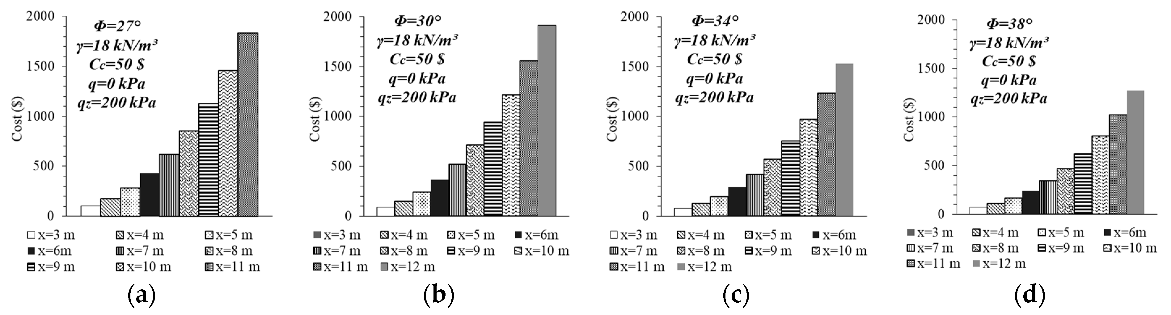
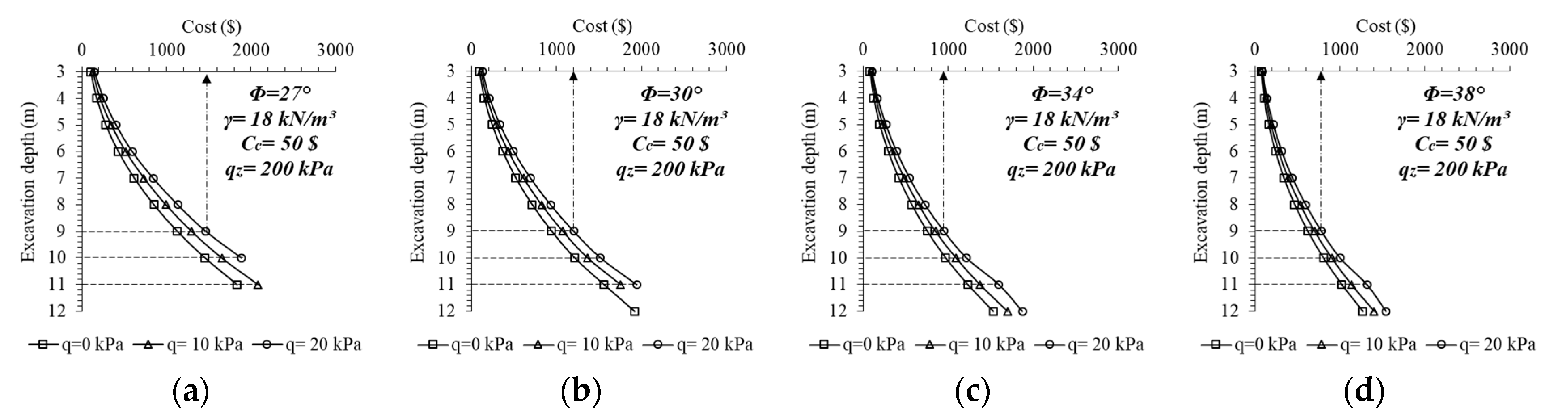
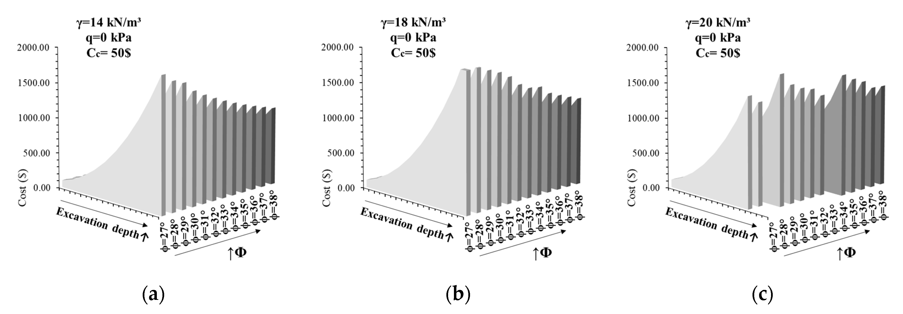
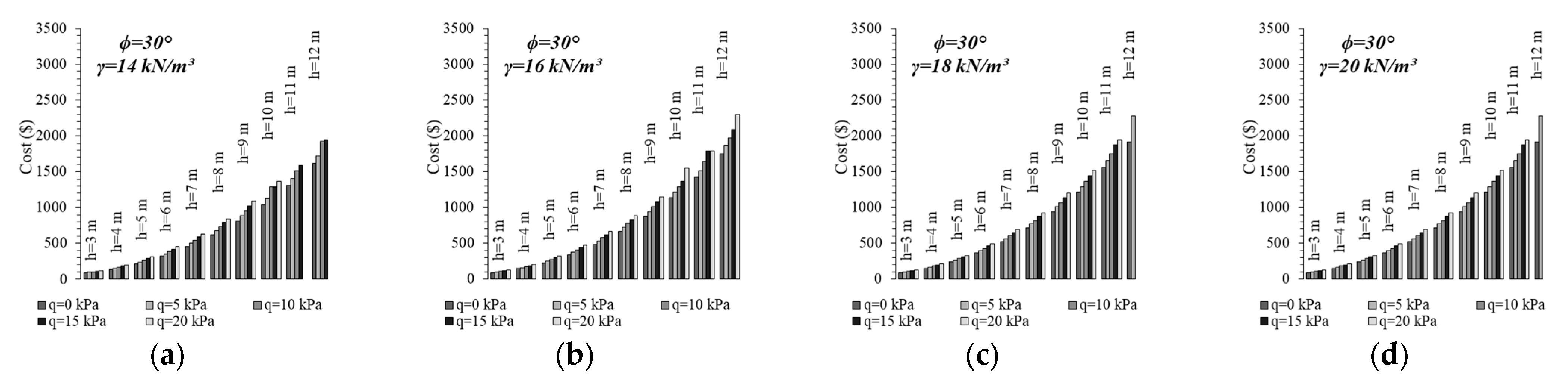
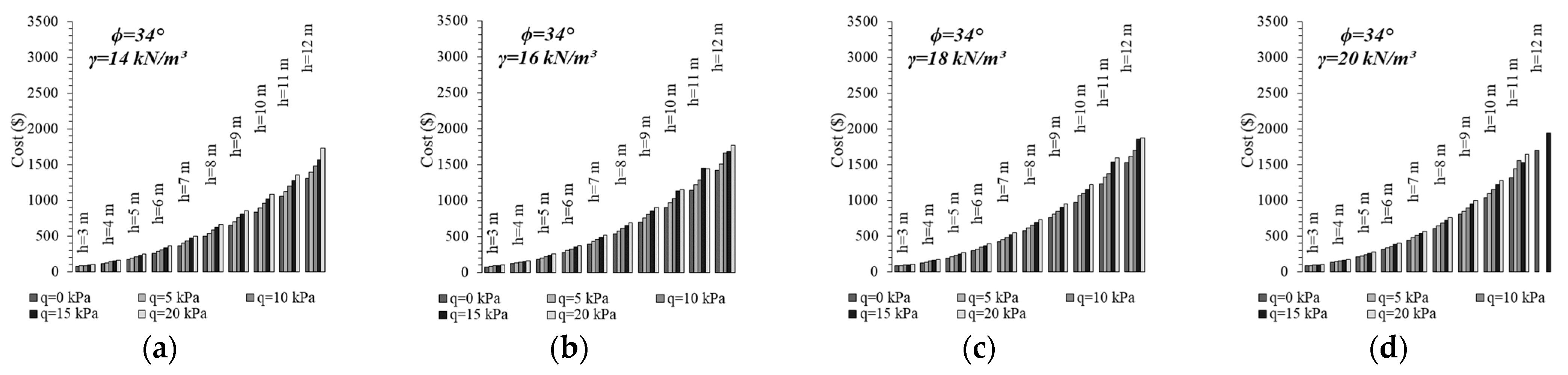
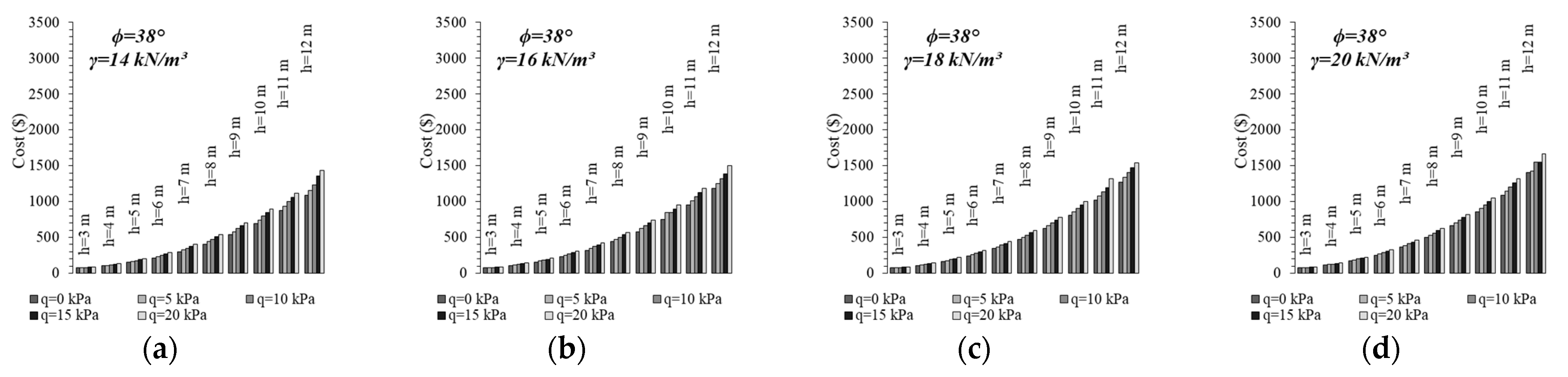
4.1.1. Investigation of the Influence of Excavation Depth Change (Case 1A)

For the evaluation of the individual influence of excavation depth on the behavior of walls, the excavation depths are selected as variables (3, 4, 5, 6, 7, 8, 9, 10, 11, and 12 m, respectively), and the other mentioned variable parameters that are shown in Table 3 are fixed as specific values. It is assumed that a surcharge load is applied adjacent to the top of the retaining system is selected as 0 and the unit weight of retained soil is selected 18 kN/m³. The unit volume cost of concrete is supposed to be USD 50. The ultimate bearing pressure of surrounding soil is preferred to be 200 kPa. The change in costs according to the increase of excavation depth is shown in Figure 4. It is seen from Figure 4 that the increase of excavation depth leads to a rise in the costs. The effect of internal friction angle change is also given in Figure 4. The internal friction angle is selected 27° (Figure 4a), 30° (Figure 4b), 34° (Figure 4c), and 38° (Figure 4d), respectively, for evaluating the dual effect degree interpretation. It can be seen from Figure 4a–d, the increase of effective friction angle causes to decrease the costs. The degree of excessive price volatility decreases with the increase of internal friction angle.

The effects of surcharge load change are also investigated. For that purpose, surcharge load is selected 0, 10, and 20 kPa, respectively. Comparative graphs are obtained using different internal friction angles (Figure 5).

The increase of the surcharge load leads to a rise in the total cost of retaining walls. However, the degree of this increase is remained lower for the smallest excavation depths. Internal friction angle values are increased from Figure 5a–d. The increase of the internal friction angle reduces the effects of surcharge load increase and decreases the final costs of retaining walls. It can be said that the effect of surcharge load change is significant for the smallest internal friction angles. Besides all these, the surcharge load change is less effective on the cost of retaining walls than the change of internal friction angle.

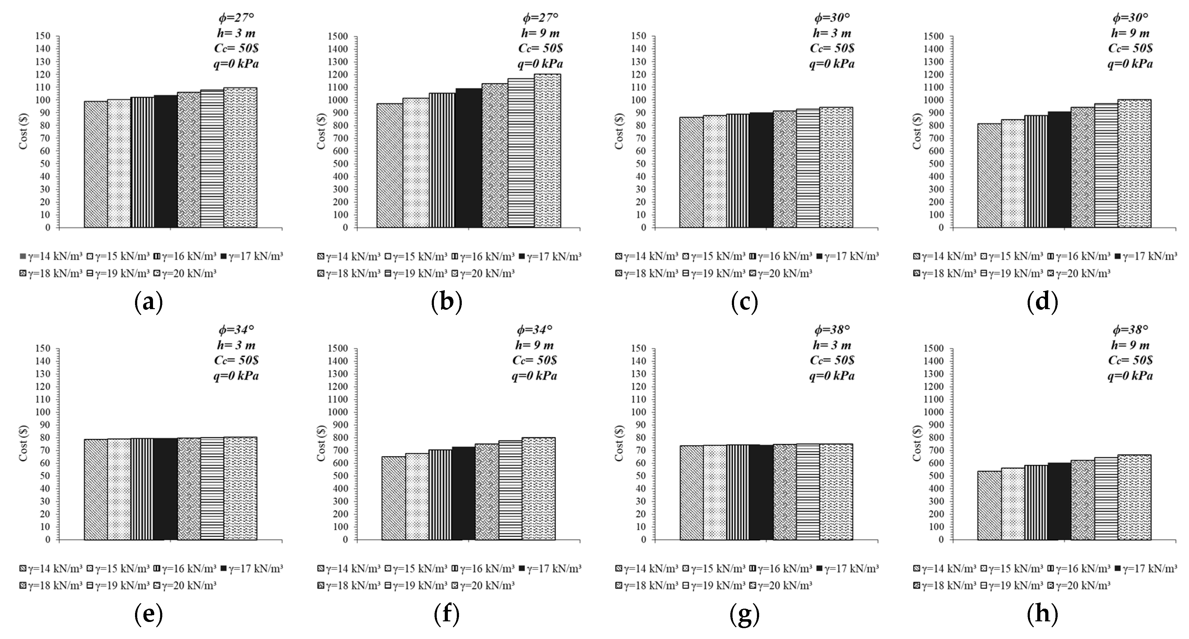
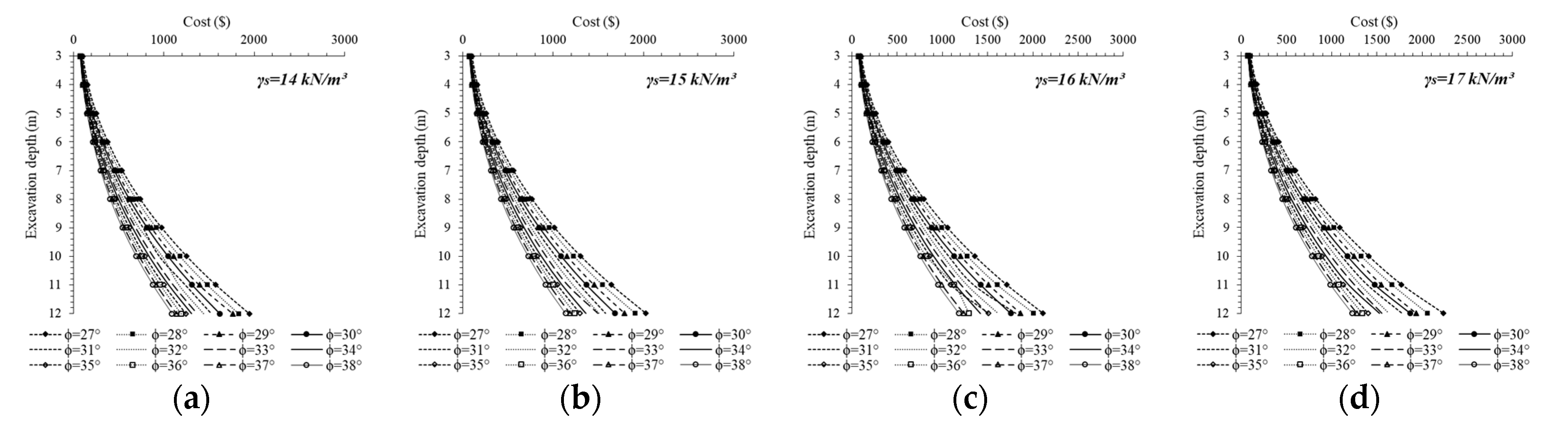
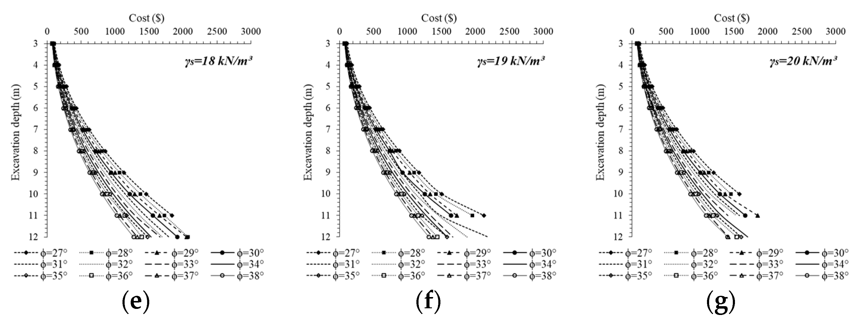
4.1.2. Investigation of the Influence of Soil Property Change (Case 1B)

The great component of the loads, which are activated at the construction of the retaining walls, mainly comprises due to lateral soil pressures. The determination of the lateral soil pressures is dependent on the physical characteristics and strength properties of the soil type. The foundation soil, backfill soil, and surrounding soil are assumed to be the same. Granular soils are preferred to perform analysis and the variants of the analyses are selected to be the unit weight, the initial friction angle, and the ultimate bearing pressure of the soil. To evaluate the effect of soil unit weight change on the cost of retaining walls, numerical analyses are conducted by the selection of specific cases. Constant project design properties are preferred to be used for defining the fictionalized cases except for the unit weight of soil. The internal friction angle is selected 27° (Figure 6a,b), 30° (Figure 6c,d), 34° (Figure 6e,f), and 38° (Figure 6g,h), respectively. The external load application is ignored, and the unit cost of concrete is assumed to be USD 50. Comparisons are made for both 3 m (Figure 6a,c,e,g) and 9 m (Figure 6b,d,f,h) excavation depths. In Figure 6, the effect of soil unit weight change against soil friction angle and excavation depth. It is significant to note that the stem depths are 3 and 9 m. When each graph is examined individually, it is seen that construction costs are raised with increasing ground unit volume weight.

The case with an internal friction angle, Φ = 27° significantly shows that the differentiation ratio of the costs gets higher with increasing excavation depth. The same trend is also encountered in other cases in Figure 6. It is calculated that the cost difference between the lower (14 kN/m³) and higher (20 kN/m³) soil unit weight is decreased depending on the increase of soil internal friction angle, especially in excavation depth at 3 m. The cost difference that is determined between the maximum and minimum soil unit weights is about 10% for the excavation depth at 3 m with Φ = 27° and around 23% at 9 m with Φ = 38°. In Figure 7, the exchange rate of construction costs dependent on the excavation depth against the internal friction angle is shown. Seven different types of soil unit weight are selected as constant values for each graph and the effects of change of soil friction angle and increase of excavation depth are monitored. The deepening of the excavation depth increased the construction costs as expected and maximum costs are achieved for the biggest friction angles. Figure 7e–g are shown for 18, 19, and 20 kN/m³ of soil unit weight, respectively. It is a remarkable condition that the construction cost could not be obtained for the excavation depth at 10, 11, and 12-m cases. This situation is the result of why there could not envisage a design that could provide technical adequateness (either geotechnical or static design safety requirements) within the limits of defined design variables.

The influence of the shear strength angle can be seen from Figure 4, Figure 5, Figure 6 and Figure 7, and also Figure 8 shows the effect of friction angle for the selected specific cases. Soil unit weight is assumed 14 (Figure 8a), 18 (Figure 8b), and 20 kN/m³ (Figure 8c), respectively.

In Figure 8, the vertical axis shows the construction costs, and the horizontal axes represent the excavation depth and the shear strength angle. It is clear to say that the increase of strength leads to a decrease in the construction costs because of a relationship between dimension changes. In Figure 8c, the decrease discontinuity which is occurring according to the increase of friction angle is broken down due to the lack of adequate design that is providing technical necessities within the limits of defined design variables.

Another investigation is the change of the ultimate bearing capacity of the foundation soil. Prototype model tests had been conducted for being experimental verification of some of the methods, but they could not produce realistic test results compared to full-scale prototypes because of scale effects. That is because the model behavior includes only a statistically small quantity of soil specimens compared with that involved with the full-scale tests. This condition cannot allow representing the whole soil medium that is going to be encountered in the field. Sandy soils can be representative examples for clarifying this situation because sand requires confinement for the generation of internal resistance [48]. Due to these reasons, in the context of this study, it is preferred to select appropriate ultimate bearing pressures at the design stage of the retaining wall to evaluate the influence on the cost and size of the system. Overall, 200, 250, 300, 350, and 400 kPa values are selected as the ultimate bearing pressure of the soil under the foundation loading condition. Different cases are fictionalized for the interpretation of the ultimate bearing capacity effect on the cost of retaining wall system. In Figure 9, two representative conditions are selected to identify the pressure effect on the cost of the wall system. In the first condition, the excavation depth is selected 9 and 12 m (Figure 9a–d). The internal friction angle and the unit weight of soil are assumed to be constant values 27° and 14 kN/m³, respectively.

In the second condition, besides the different excavation depths, surcharge load change is also evaluated (Figure 9a–d). It should be noted that the vertical axes have different numerical values in the plotted graphs. Figure 9a,b show that the increase of the excavation depth rises the costs of the whole wall system but there is no effect of the change of the ultimate bearing capacity on the costs if the surcharge load is not applied to the top of the wall. The increase of the surcharge load to 20 kPa has increased wall costs approximately 2% for the small values of ultimate bearing capacity (Figure 9c,d) but the increase of ultimate bearing capacity provides to equalize the costs. Figure 10 illustrates the influence of soil unit weight coupled with the surcharge load change on the costs. The excavation depth and the internal friction angle are selected as 9 m and 29°, respectively. The unit weight of the soil is identified as 14 kN/m³ in Figure 10a,c and 17 kN/m³ in Figure 10b,d. The surcharge load that is applied on the backfill side is assumed to be 0 and 20 kPa, respectively. The increase of soil unit weight does not influence the costs if the surcharge load is not applied. The increase in the surcharge load leads to rising costs for both selected unit weights. However, the rise of ultimate bearing pressure to a limit level the costs remain constant. Depending on the selected soil parameters and specified cases, this limit level of the ultimate surcharge load can be said 300 kPa.

Another case is fictionalized for designating the effect ratio and for evaluating the variance behavior of wall costs according to the increase of excavation depth. The excavation depth is assumed 12 m and internal friction of the soil is preferred to use 29°. The unit weight of the soil is selected 14 and 17 kN/m³, respectively. Surcharge load is also selected as a variant. Comparisons are conducted for Figure 10 and Figure 11. Unlike Figure 10a, the deepening of excavation causes to raise costs, approximately 3%, for the smallest ultimate bearing pressure. The increase of soil unit weight does not affect the costs similarly for both excavation depths.

The increase of soil unit weight and surcharge load together lead to obtaining the same behavior trend for both selected excavation depths. It can be said that the attainment of the reliable value of the ultimate bearing pressure of the soil under the application of wall foundation loads constitutes a different problem that has to be solved with an integrated perspective containing both geotechnical and structural engineering disciplines. In the study, this phenomenon is parametrically discussed with the assumption of various cases, but it is thought that the evaluations about the change of the ultimate bearing pressure cannot be generalized. The dependent factors of bearing capacity are still the concern of studies and there is not a common study that has been proved yet.

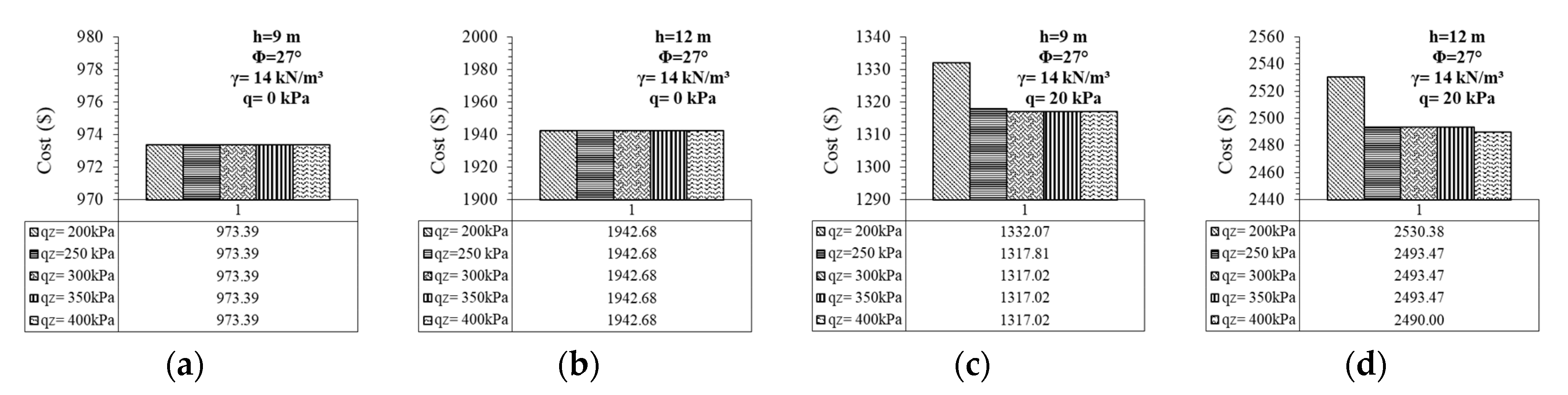
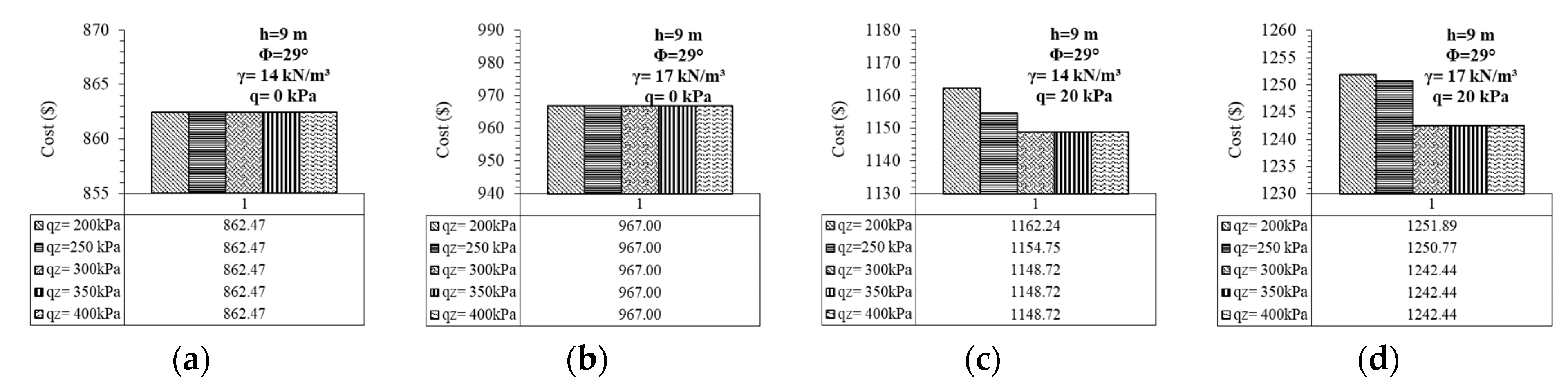
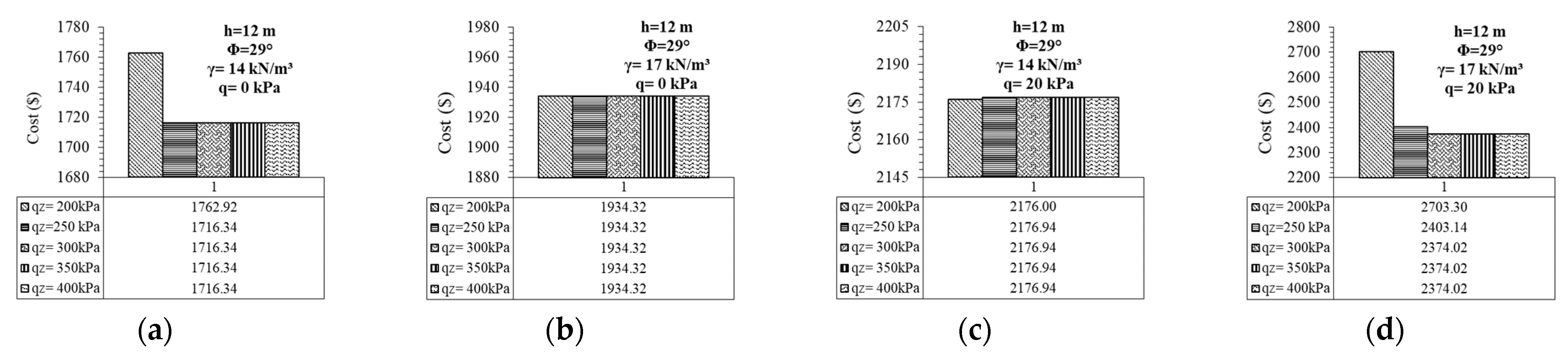
4.1.3. Investigation of the Influence of Surcharge Loading Condition Change (Case 1C)

The surcharge that is affected by the soil surface from the top of the wall system is assumed to be infinite and uniform. Five different loading conditions are fictionalized for evaluating the cost effects. First, there is no surcharge on the cantilever RC-retaining wall system. Next, it is assumed to apply 5, 10, 15, and 20 kPa surcharge loads, respectively. In Figure 12, Figure 13, Figure 14 and Figure 15, the change of cost according to the change of surcharge magnitude is given with the internal friction angles, Φ = 27°, Φ = 30°, Φ = 34°, and Φ = 38° respectively. These graphs also represent the integrated effects of the variants together. It is expected that the increment of the surcharge loading causes to rise of the active pressures that are acting to the wall as a distributing lateral load. This is the reason for extending the dimensions of the wall for reaching stability requirements. Furthermore, the rise of surcharge load against the increase of soil unit weight (Figure 12a–d) leads to a decrease in costs, especially for smaller degrees of friction angle.

For all the fictionalized cases, the increase of active surcharge load leads to a rise in costs. However, the rising ratio of the costs is smaller for more competent soils. This means that the improvement of soil physical conditions and strength properties causes to decrease in construction works and costs. The minimum cost change occurred in the case of the biggest internal friction angle and unit soil weight condition.

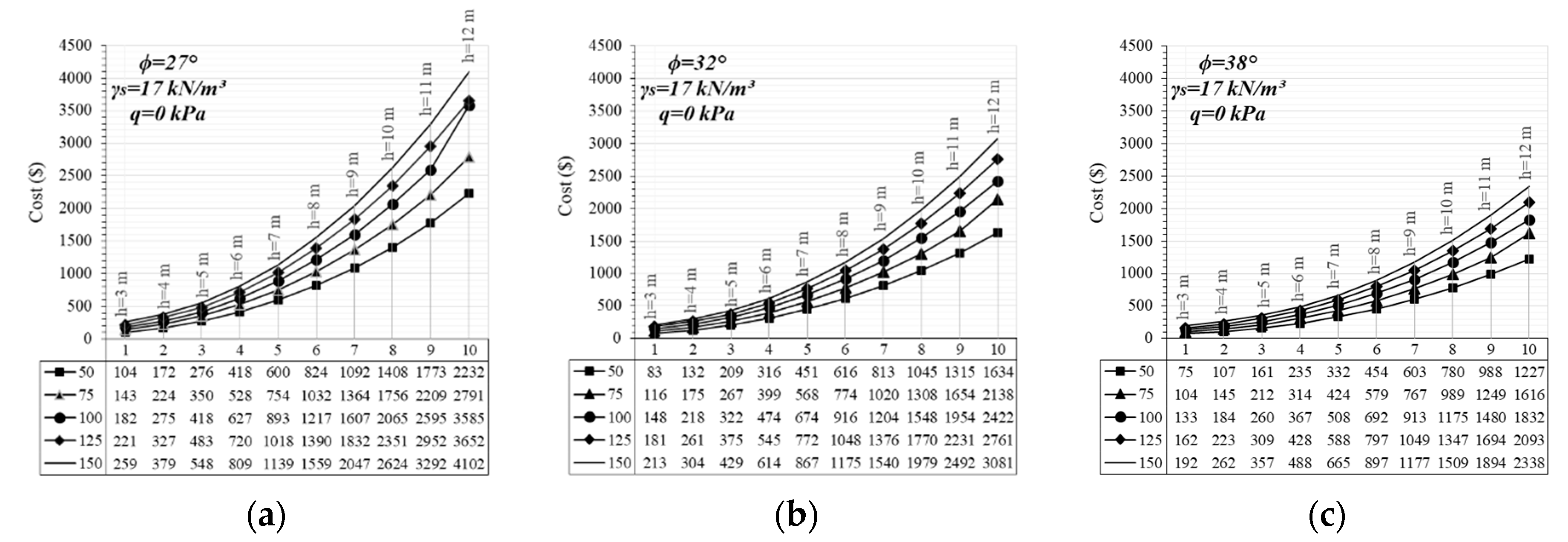
4.1.4. Investigation of the Influence of Unit Cost of Concrete Change (Case 1D)

The unit price of the concrete is selected as an important factor because the actual cost of the concrete differs by region due to the ingredients and manufacturing costs it. The unit cost of the concrete material is assumed to be USD 50, USD 75, USD 100, USD 125, and USD 150, respectively. Three specific cases are selected for the investigation of total cost change according to the concrete material cost. In Figure 16, the internal friction angle of the soil is selected 27, 32, and 38°, respectively. It is assumed that no surcharge load is applied to the system and the unit weight of the soil is defined as 17 kN/m³. The excavation depth change is also taken into account. As shown in Figure 16a,c, it can be said that the increase in concrete costs is cost-effective for the condition in which the soil is less strong. The improvement of the soil properties leads to lessening the effect of concrete cost and straitens the effective rate on the total cost. The cost increase ratio due to the rise of the unit cost of concrete is reduced with the decrease of excavation depth.

4.2. Numerical Dimension Analyses of Cantilever RC-Retaining Walls (Case 2)

In the second part of the study, the effects of excavation depth, soil parameters, environmental conditions, and unit costs of concrete are investigated to evaluate the change of dimensions of retaining walls at the design stage. Case 2 is divided into subgroups for the individual effects of design components (Cases 2A, 2B, and 2C). Later, the dual effects of variables are investigated with the selection of specific cases.

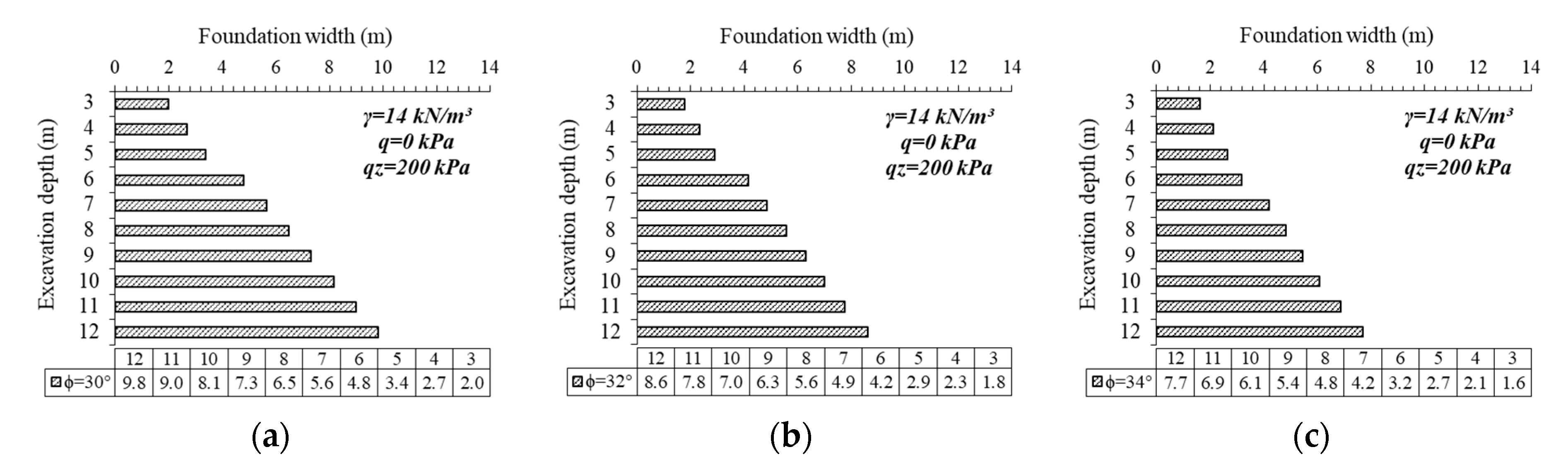
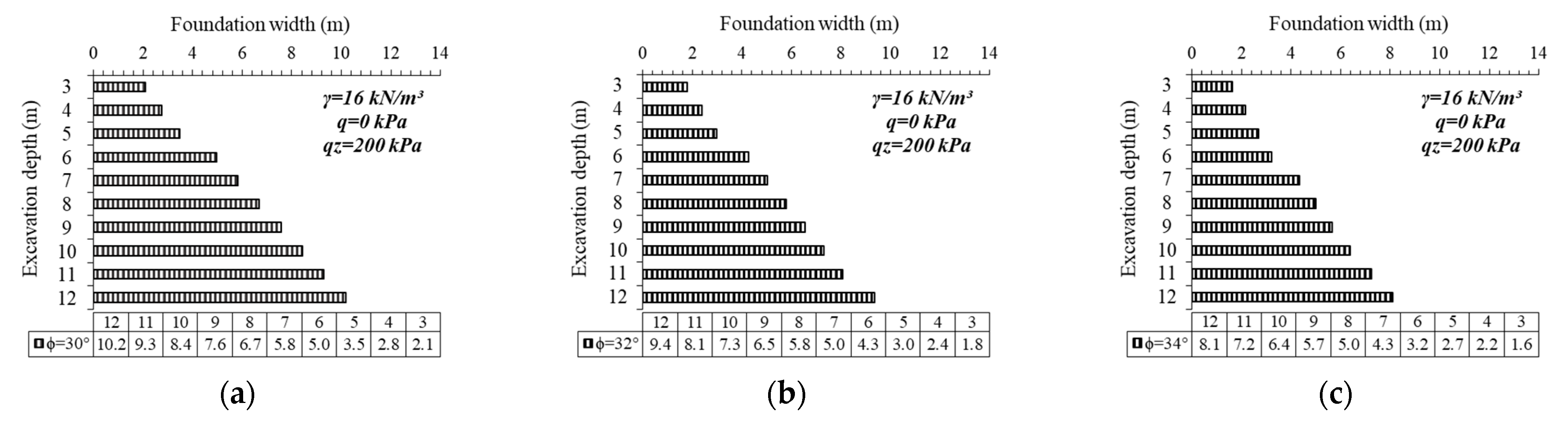
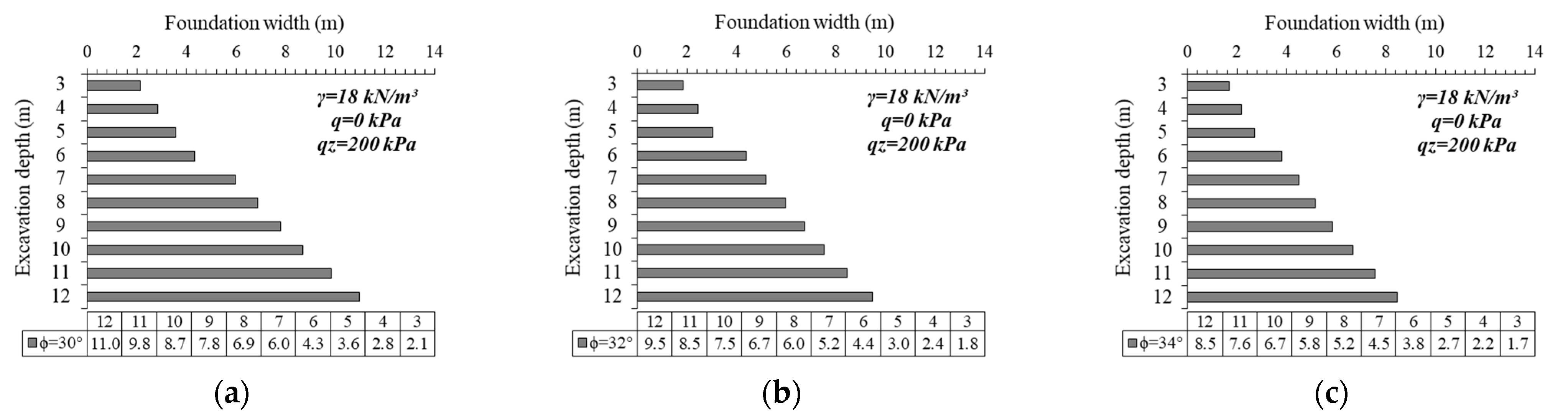
4.2.1. Investigation of the Influence of Excavation Depth Change (Case 2A)

The excavation depth is set to 3, 4, 5, 6, 7, 8, 9, 10, 11, and 12 m, respectively, and the analyses are performed to achieve design comparison with the application of HS. The influence of excavation depth change on the design of reinforced concrete retaining walls is investigated according to the selected reference cases with the use of dual parameter comparison. The change of the design dimensions is evaluated by the use of foundation width that is consisted of the sum of heel, toe, and wall stem widths. The heel width has been restricted with the use of a specific value (10 m). In Figure 17, Figure 18 and Figure 19, the influence of excavation depth against foundation width is given according to the differentiation of soil unit weights. In Figure 17, Figure 18 and Figure 19, the unit weight of the soil is assumed to be 14, 16, and 18 kN/m³. On the other hand, the change of soil internal friction angle is also considered with subdivisions of the related figures. Overall, 30, 32, and 34° of internal friction angle are selected for the selected cases. The surcharge load and the ultimate bearing pressure of the soil parameters are selected constant values (q = 0 kPa and q_z = 200 kPa). In Figure 17, Figure 18 and Figure 19, it can be seen that the increase of foundation depth leads to wide foundation base width for all the selected cases due to the increase of unbalanced active forces. The width of the foundation has been increased to ensure stability conditions according to the optimization technique. Optimization has been performed to evaluate average design according to the minimum costs and minimum dimensions of the wall systems. The increased ratio of the foundation width is particularly bigger for relatively loose soils (for example, γ = 14 kN/m³ and Φ = 30°). The rise of soil strength leads to a decrease in the foundation base width. In Figure 18 and Figure 19, the change of foundation width is investigated for 16 and 17 kN/m³ of soil unit weight, respectively. A similar trend is achieved for the increase of foundation width with the deepening of the excavation for Figure 18 and Figure 19.

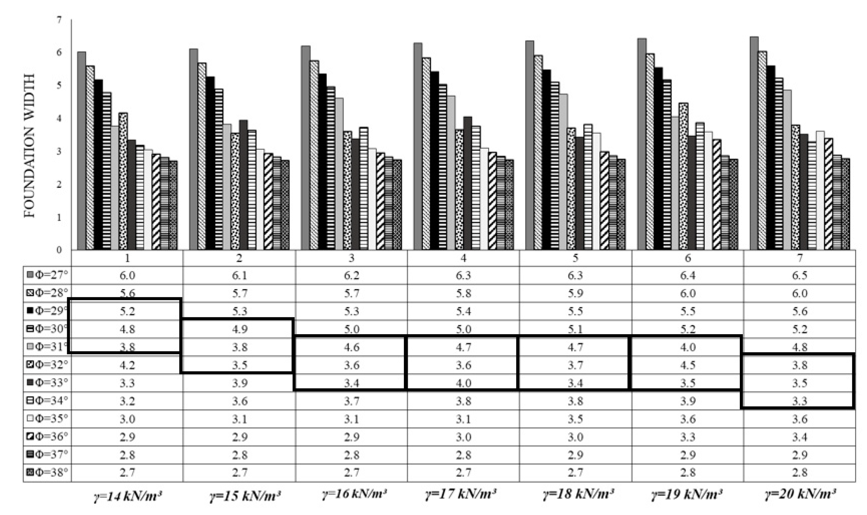
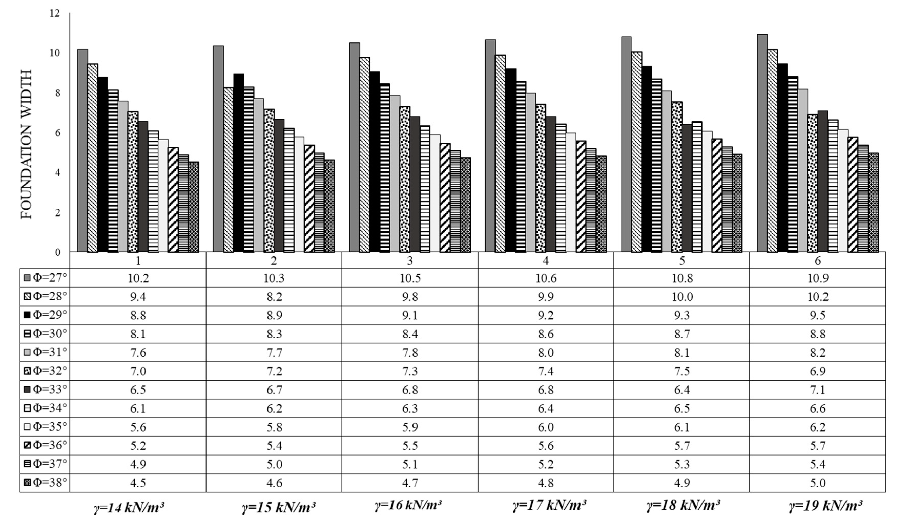
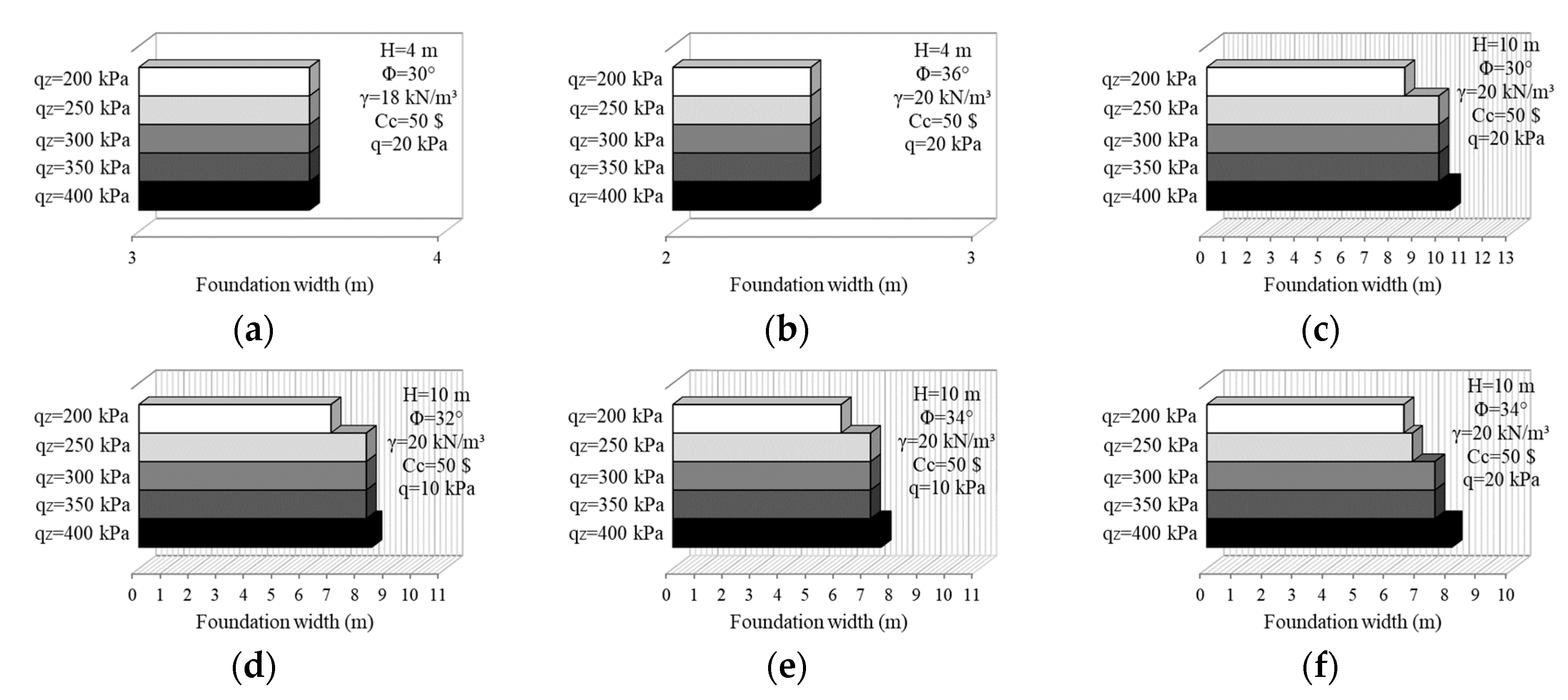
4.2.2. Investigation of the Influence of Soil Property Change (Case 2B)

The effects of the soil properties in the design of the wall are investigated by the use of different internal friction angles, unit weights, and ultimate bearing pressure values of the foundation with medium soil. Optimization analyses are conducted to acquire the width of the foundation base and integrated evaluations are shown in Figure 20, Figure 21 and Figure 22.

In Figure 20 and Figure 21, the differentiation of foundation width is investigated by the use of twelve (12) internal friction angles (27, 28, 29, 30, 31, 32, 33, 34, 35, 36, 37, and 38°) and seven (7) different soil unit weights (14, 15, 16, 17, 18, 19, and 20 kN/m³). The excavation depth is selected 6 and 10 m for Figure 20 and Figure 21, respectively. The surcharge load is assumed not to be applied and the ultimate bearing pressure of the foundation soil is supposed 300 kPa for the cases analyzed. In Figure 20 and Figure 21, it can be seen that the increase of the soil strength causes foundation base width to become narrow as is expected. The increase of the unit weight of the soil causes to raise the lateral active pressures acting on the wall sections. Therefore, the stability of the wall tried to be ensured by the enlargement of the wall foundation. Besides, the influence rate of the soil unit weight on the dimensions of the wall system is smaller than that of the soil strength when comparisons are conducted for a unit increase of related parameters.

Especially for Figure 20, the decrease of wall foundation base width against the increase of internal friction angle has exhibited irregularities for specific cases. These cases are shown with rectangular boundaries in Figure 20. The comparison of the traditional pre-design method and optimization approach of reinforced concrete retaining walls is explained with this situation. In the traditional pre-design method of retaining walls, the designer approximately selects the base and stem dimensions, checks them against stability. If the design is not safe, a trial and error procedure is applied. Then the allowable limits of the bearing pressure are computed, base shear and moment are evaluated. Provided that the largeness of base shear, it can be preferred to increase the embedment depth until the case satisfies. It will be proper to reduce the stem height to procure constant wall height. On the other hand, if the foundation base thickness is adequate, the toe and heel steel requirements are computed. Consequently, the traditional pre-design of reinforced concrete retaining walls primarily searches for the geotechnical stability criteria and structural design requirements for the second stage. It can be shown that this pre-design process involves much busywork and seems not to be convenient concerning economy, sizing, and duration [48]. Compared to the conventional design method, the optimization techniques enable an integrated loop considering both geotechnical stability and structural requirements simultaneously and ensure security and economy together. Two different structural materials with dissimilar mechanical properties and costs are used at the generation stage of structural calculations of optimization analysis.

For the attainment of the stability conditions, it is necessary to use the concrete material that is relatively more cost-effective than the steel material. On the contrary, if the design needs to extend the boundaries of the wall too large and/or thick to ensure stability conditions, the cost of whole concrete sections will have been over the expected limits. Under this circumstance, an optimization procedure allows the wall sections to become narrow and raise the density of steel material. Generally, if the cost of the concrete material is higher than the steel one for the proposed design of the wall, the optimization technique will allow reducing the foundation base width or other sections of the wall. The irregularity in Figure 20 shows that the minimization of concrete and steel material costs is also achieved except for geotechnical stability. In Figure 22, the influence of ultimate soil pressure change on the foundation width is also investigated and special graphs are illustrated for selected cases. Ultimate soil pressure is assumed to be 200, 250, 300, 350, and 400 kPa for all the selected cases. In Figure 22a,b, the depth of the excavation is selected 4 m, the surcharge load is assumed to be 20 kPa and the unit cost of the concrete is selected USD 50. The internal friction angle is 30, 36° and the unit weight of the soil is 18, 20 kN/m³, respectively. It can be said that for relatively small depths of excavation, the change of ultimate soil pressure does not affect the size of the wall system. This is because the active pressures are smaller than the resisting forces till a boundary excavation depth. Different from this situation, Figure 22c–f) present a dissimilar behavior against the change of ultimate soil pressure. The excavation depth is 10 m, the unit weight of the soil is 20 kN/m³, and the unit cost of the concrete is USD 50 for these cases. The internal friction angle is 30-32-34° for 20c-20d-20e/20f subdivisions of Figure 22, respectively. The increase of excavation depth associated with the increase in ultimate soil pressure leads to a change in the size of the foundation base due to the raised active pressures and stability requirements. Furthermore, the increase of surcharge load (Figure 22e,f) caused to enlarge the foundation width.

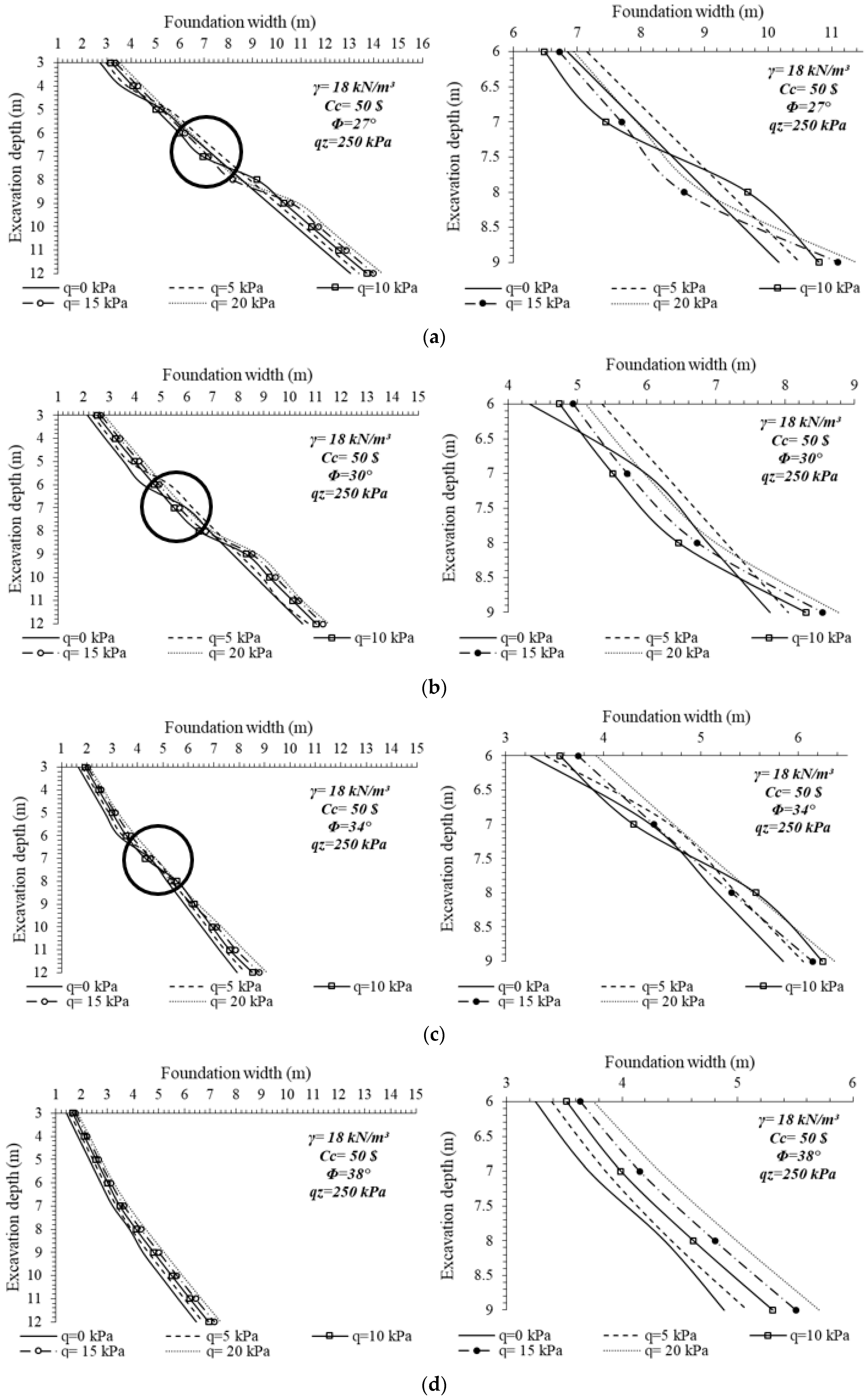
4.2.3. Investigation of the Influence of Surcharge Loading Condition Change (Case 2C)

Sizing analyses of reinforced concrete retaining walls are conducted considering that the surcharge load from the top of the wall system is infinite and uniform. Similar to the cost analyses, five different loading conditions are fictionalized for evaluating the cost effects (q = 0, 5, 10, 15, 20 kPa). The change of the foundation width against the surcharge load is shown in Figure 23. It is expected that the increment of the surcharge loading causes enlarging the foundation width because of the resultant increase of active sliding pressures. The increase of the sliding forces caused by surcharge is directly affected by the lateral earth coefficient of the soil. Accordingly, it is important to see the sizing differentiation induced by the soil strength. This situation is illustrated in Figure 23a–d for the case that initial soil friction angle is Φ = 27°, Φ = 30°, Φ = 34°, and Φ = 38°, respectively. The subdivisions of the figure are comprised of two different graphs. The first graph represents the change of foundation width against the whole excavation depth with the differentiation of various surcharge loads. The second graph is the detailed graph that represents the unexpected behavior tendency about the change of foundation width especially for the loading stages equal to and bigger than 10 kPa. It may be said that the depths between 7 and 9 m are critical design depths for loose to medium dense frictional soils because there has become a structural design change between these depths for all the cases. This condition is due to the optimization technique which searches for the results of the minimum material costs against minimum dimensions. Figure 23d represents dense frictional soil behavior under the change of surcharge conditions. The increase of soil strength reduces the dimensions of the wall foundation as shown in Figure 23d. According to this situation, the concrete volume cost used for the proposed design of the wall system has been smaller than the cost of steel for the alternative design.

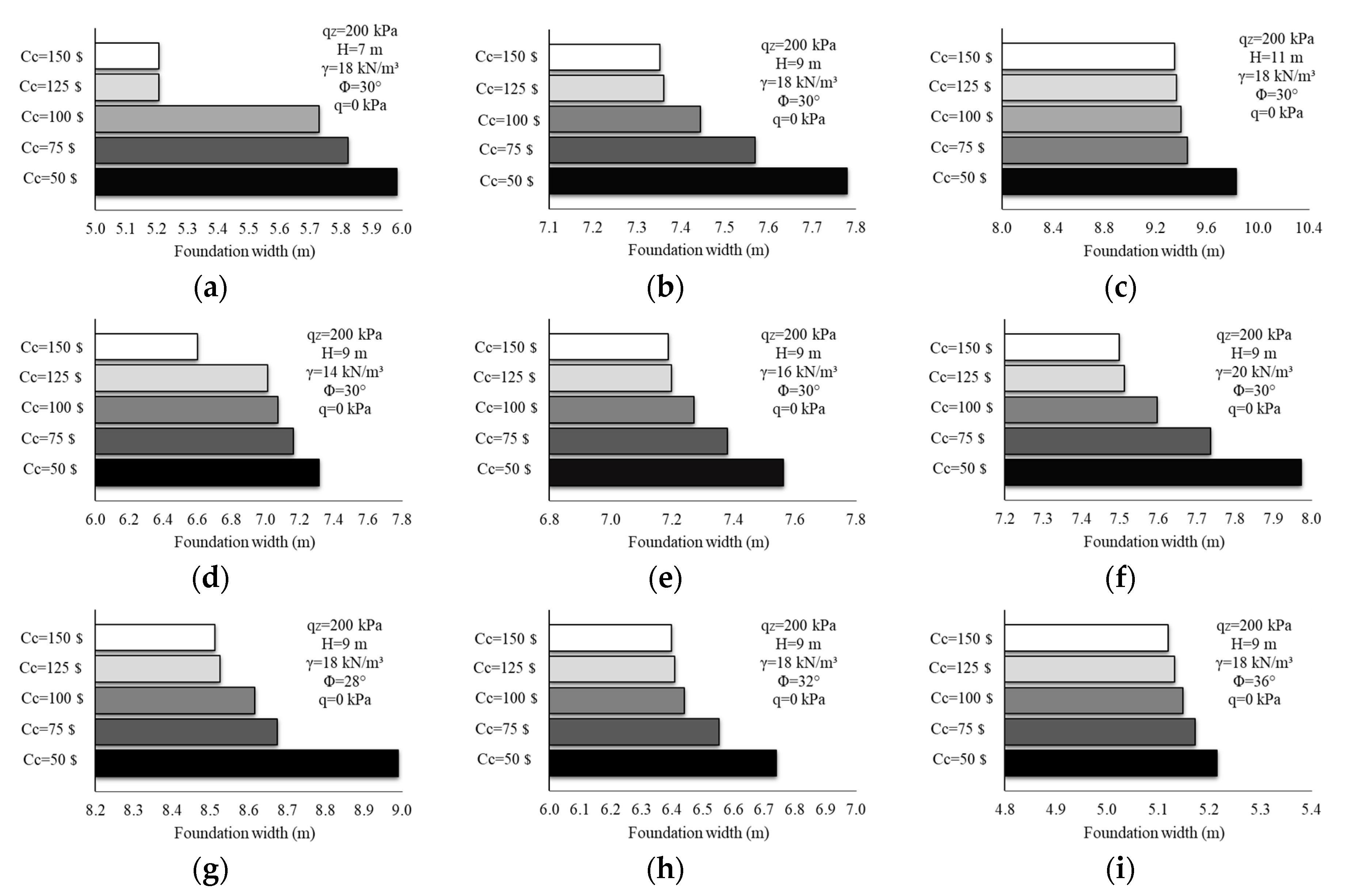
4.2.4. Investigation of the Influence of Concrete Cost Change (Case 2D)

Concrete and steel are the main components of retaining wall construction which can be defined as two different structural materials that have various costs according to the related region. Due to this reason, the unit cost of these materials plays a significant role in the optimum design. To evaluate this situation, dual effect comparisons are conducted, and the unit cost of the concrete is set to be USD 50, USD 75, USD 100, USD 125, and USD 150, respectively. Firstly, the concrete cost effect is acquired with the change of excavation depths (Figure 24a–c). The ultimate base pressure 200 kPa, internal friction angle 30°, unit weight of the soil 18 kN/m^3, and the surcharge load 0 kPa are assumed and shown for 7-, 9-, and 11-meter’s excavation depths in Figure 24a–c. In general, the increase of the excavation depth leads to an increase of foundation dimensions, but the rates of increase are differentiated according to the change of unit cost of concrete material. This means that the influence of the increase of concrete cost is especially significant for relatively smaller excavation depths for the cases. In Figure 24a, the excavation depth is assumed 7 m. The minimum charge of the unit cost of concrete leads the designs to be constructed predominantly with a further volume of concrete. The dimension differentiation ratio between the prices that are used as the upper and lower limits of the concrete unit cost is calculated approximately 15% for this specific case. The increment of the excavation width reduces this ratio nearly to 6%. Furthermore, after a specific limit cost of concrete, the design is not changed (for H = 7 m the limit cost is USD 125, for H = 9 m the limit cost is USD 125 and for H = 11 m the limit cost is nearly USD 75). The effect of soil unit weight change against the cost of concrete influence is shown in Figure 24d–f. The depth of excavation is assumed 9 m, the ultimate soil pressure is taken as 200 kN/m², the internal friction angle is 30°, and no surcharge load is applied. Overall, 14, 16, 40 kN/m³ values are taken as the soil unit weight values, respectively. The increase of the unit weight of the soil causes to rise of the unbalanced forces of the system, and it leads to an increase in the width of the foundation as expected. This means that the increment of the unit cost of concrete contributes the dimensions to be the same after a limit cost value. The maximum dimension change occurs 10% for the condition that the dual effects of unit weight of soil and the cost of concrete are taken into account. In Figure 24g,h,j, the influence of internal friction angle change against the unit cost of concrete is investigated. Constant parameters are selected as the same as the previous case, but the internal friction angles are assumed to be 28, 32, 36°, respectively. Maximum dimension change has occurred for the loosest soil conditions, and the influence ratio of the change is calculated maximum of 7%. The improvement of the soil properties leads to lessening the effect of concrete cost and straitens the effective rate on the total cost. Consequently, a similar behavior trend is exhibited for all the selected cases. The rise of concrete cost leads to an increase in steel amount through the design process to reduce the wall costs with the achievement of minimum sizing.

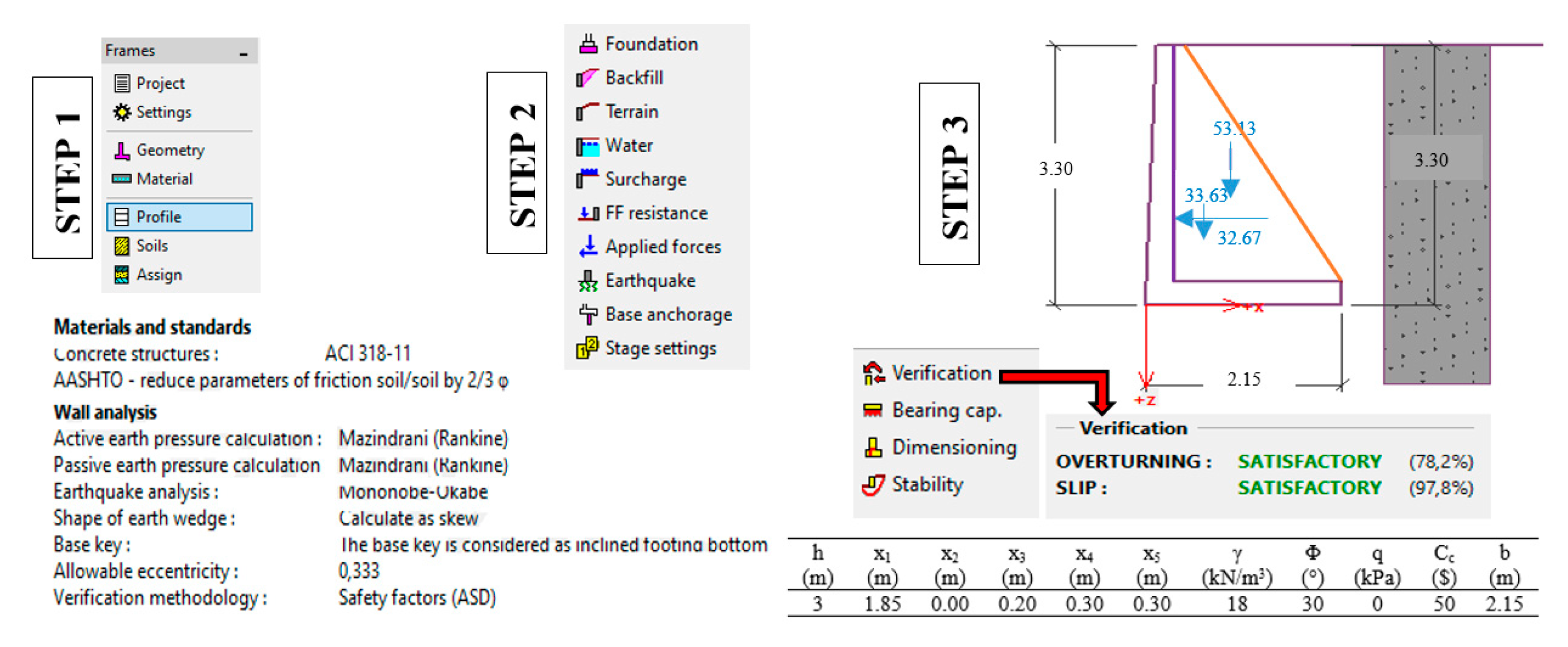
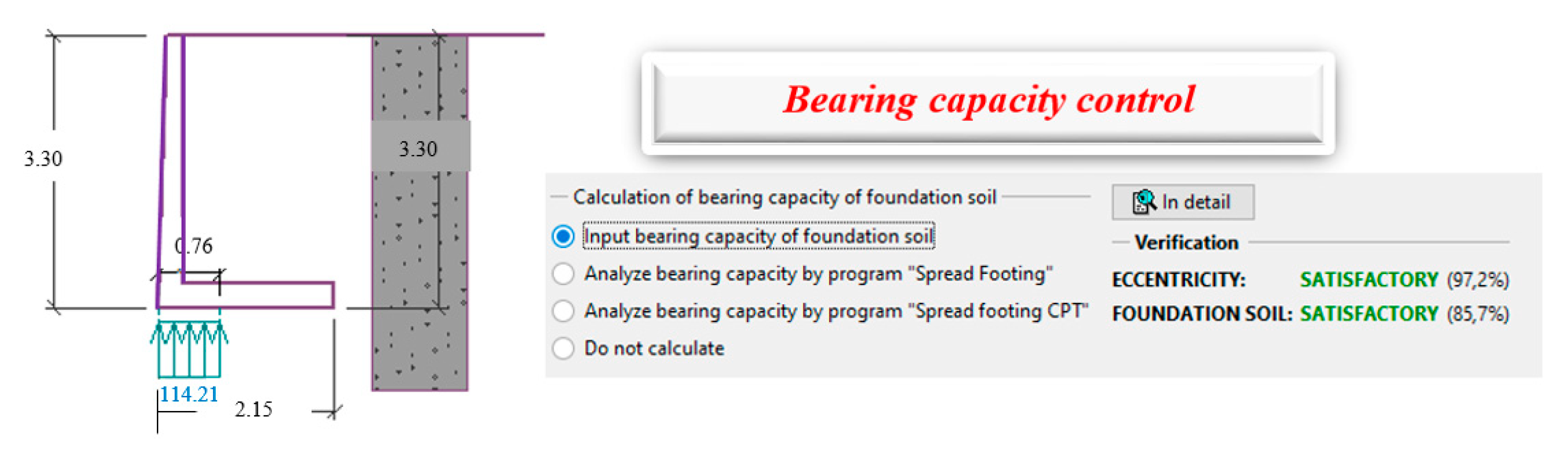
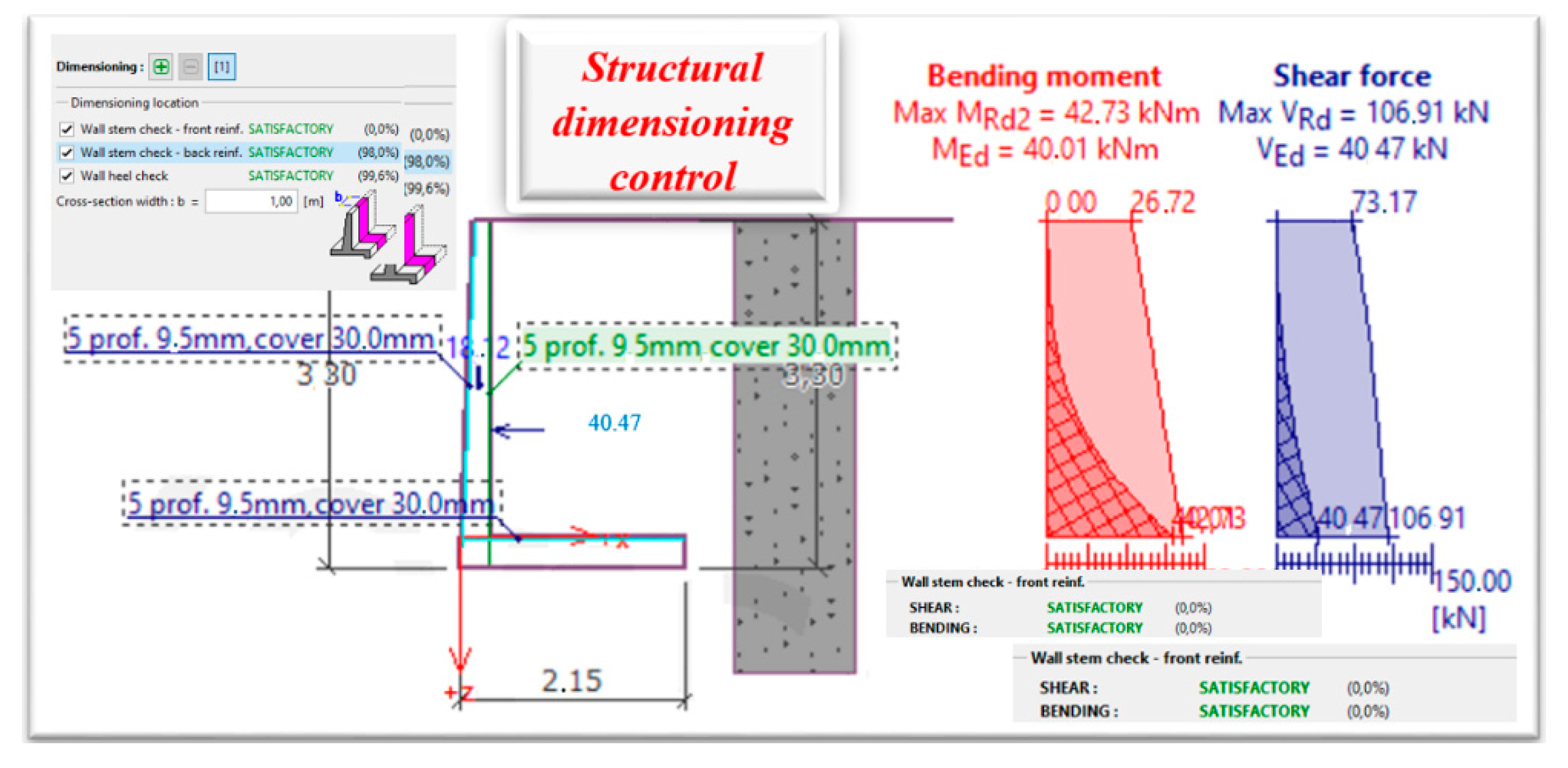
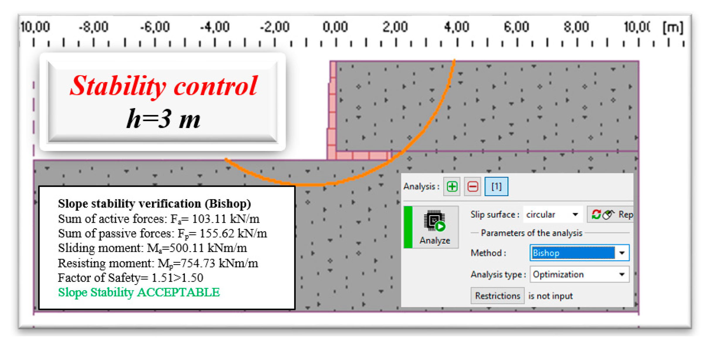
4.3. Numerical Analysis with Geo5 Software

To validate the design procedure arranged with the use of Harmony Search Algorithm for reinforced concrete retaining walls, numerical analyses were conducted using the commercial software Geo5 that is an effective software package depending on both analytical and finite element methods and developed for solving geotechnical problems like slope stability, foundations, retaining walls, and so on. The analytical method allows the users not only to design but also to check structure stability situations quickly and efficiently. The analytically designed structure is transferred to the finite element model for the overall analysis of the whole structure. This transmission process saves the computational time of designers and compares two independent solutions, so it increases the safety of the design [72,73,74,75,76,77]. Within the software context, there are 28 different moduli (like abutment, anti-slide pile, beam, cantilever wall, gabion, spread footing, and so on.) which include different geotechnical design structures individually. However, all moduli can transfer or communicate with each other and form an integrated total package. Besides, worldwide usage is ensured with the existence of design conditions proposed by various geotechnical (Caquot-Kerisel, Coulomb, Rankine, Absi, and so on) and structural (EN 1992-1-1, ACI 318, BS8110:1997 and so on) standards embedded into the software.

In the study, depending on the previously mentioned properties of the software, Geo5 version 2021 is preferred to be used to validate the suggested design dimensions. The free version of the software has been used without restrictions of the program, to analyze the selected specific cases. The shear strength angle and the unit weight of the foundation and backfill soil are assumed to be 30° and 18 kN/m³, respectively, and no surcharge loading is considered. All the envisaged cases that are analyzed with HS optimization logic have been also solved with Geo5 software, but the details of the analysis for the 3-m excavation depth only have been illustrated. The geotechnical and structural design standards are selected in the first step of the analyses conducted with Geo5 (Figure 25). The structural design requirements are modeled depending on the limitation of ACI 318, and AASHTO is used to model geotechnical standards. The active and passive earth pressure calculations are arranged to be performed with the use of Rankine theory. Besides, the foreseen geometry of the wall system, the properties of the soil formation, and the stratification situation of the foundation soil medium are defined at the first stage. The second stage of the analyses includes additional situations like the existence of the water table or external forces. In the context of the analyses considered for this section, there is not any necessary condition to define. The third step includes the verification of overturning and sliding safety, bearing capacity adequateness, structural dimensioning control, and overall stability research with slope analyses.

The HS optimization results for 3-m excavation depth is given in Figure 26. The total height of the wall is determined as 3.3-m by the sum of the excavation depth and the thickness of the foundation base. The L-shaped section is obtained without the toe length, and the heel length is suggested to be 1.85 m. The thickness of the stem at the top and bottom is calculated 0.2 and 0.3 m, respectively. Figure 26 reflects the bearing capacity adequateness for the envisaged dimensioning of the design. The eccentricity and foundation soil situations are found to be satisfactory.

The next step of the verification process is the control of structural dimensioning in terms of shear and bending conditions of wall stem and wall heel. In this context, Figure 27 shows that the front and back reinforcement and heel reinforcement are found to be adequate in terms of shear and bending moment.

The last step of the verification process is the control of overall stability (FoS_os) in terms of slope stability. Various methods such as the Bishop, Morgenstern-Price, Janbu, Fellenius/Petterson, and Spencer method, are presented to check the stability conditions of the wall depending on standard, optimization, and grid search analysis types. The analysis type “optimization” is thought to be perfect to compare the results of the optimization analyses conducted with HS. Furthermore, the Bishop method has been used to check the stability situation of the wall system and the circular slip surface assumption is made. The results of the analysis are presented in Figure 28. The boundary safety number is 1.5 for the Bishop method and the envisaged dimensioning of the wall system has ensured a 1.51 safety number. This situation reflects the applicability of the HS method for being an advantageous alternative and fast solution technique by considering lots of situations and conditions at the same time.

The application of the same procedure is exemplified for various excavation depths based on the suggested dimensions by the HS analyses.

Table 4. The comparison of the results of the HS algorithm and Geo5 analyses.

The Results of the HS Algorithm						FoS Values Determined via Geo5 Analysis
h (m)	x1 (m)	x2 (m)	x3 (m)	x4 (m)	x5 (m)	FoSs	FoSot	FoSbc	FoSos
3	1.85	0.00	0.20	0.30	0.30	2.41	2.05	4.08	1.51
4	2.52	0.00	0.20	0.31	0.30	2.40	2.04	4.08	1.53
5	3.13	0.00	0.20	0.43	0.31	2.46	2.07	4.11	1.50
6	3.76	0.00	0.20	0.55	0.38	2.43	2.02	3.96	1.51
7	4.25	1.00	0.20	0.74	0.41	2.43	1.87	3.08	1.50
8	4.84	1.14	0.20	0.90	0.49	2.44	1.87	3.07	1.52
9	5.42	1.29	0.20	1.07	0.57	2.43	1.87	3.05	1.52
10	6.00	1.43	0.20	1.26	0.66	2.42	1.87	3.03	1.51
11	6.92	1.62	0.20	1.29	0.79	2.40	1.86	3.01	1.53
12	7.28	2.08	0.20	1.61	0.89	2.40	1.84	3.00	1.52

shows the results of the comparisons that are conducted between the performance of Geo5 software analysis and HS solutions through the determination of safety factor values for sliding, overturning, bearing capacity, and also slope stability (overall failure). The factor of safety values for sliding, overturning, bearing capacity, and overall stability is applied 1.5, 1.5, 3, and 1.5, respectively, for HS analyses as shown in Table 3.

HS analyses are aimed to ensure the lateral and vertical forces and moment equilibrium for reaching the limit state depending on the foreseen factor of safety values although Geo5 analyses are searching for the total factor of safety values depending on the envisaged dimensions. Therefore, it can be a measurable parameter of the validation process of the HS analyses to compare the determining factor of safety values of Geo5 analyses with the limit factor of safety values. It can be seen that the factor of safety values against sliding, overturning, bearing capacity, and also overall stability is exceedingly supplied by Geo5 analyses. These results show that the optimization analyses conducted with the application of the HS algorithm are both fast, cost-effective, and satisfactory for the solution of reinforced concrete retaining wall problems.

5. Conclusions

In the research, design optimization of cantilever RC-retaining walls has been attempted by performing an analysis with regard to the minimization of sizing via cost control. A huge number of (105,000) analyses have been performed with HS to evaluate the effects of excavation depth, soil properties, cost of materials, and loading conditions on the dimensional requirements of supporting cantilever RC-retaining wall systems. Individual and dual effects of the influencer parameters are both investigated. Results of the optimization analysis are compared by interpretations and logic against the traditional pre-design method and also a practical software.

The outcomes of this study can be mentioned below:

• For the fictionalized cases, the increase of soil strength properties leads to a decrease in the costs, and maybe after a limit value of friction angle, the necessity of constructing a wall system is disappeared.
• The increase of the surcharge load causes to increase in the total cost of retaining walls, but the degree of this increase remains low for shallow excavation depths.
• The increase of the surcharge load raises costs for selected unit weights, but with the rise of ultimate bearing pressure to a limit level the costs remain constant.
• The increase of foundation depth widens the foundation base width for all the selected cases due to the increase of unbalanced active forces. In such a case, the maximum costs are achieved for the biggest friction angles.
• The increase of concrete costs is cost-effective for the condition in which the soil is less strong. Besides this, the improvement of the soil properties tends to lessen the effect of concrete cost and straitens the effective rate on the total cost. The cost increase ratio due to the rise of the unit cost of concrete is reduced with the decrease of excavation depth.
• In some cases, the rise of concrete prices directs the design to straighten the section of the wall and enhance steel density to ensure stability.
• The comparison of HS optimization analysis results with the results of a geotechnical engineering software proves the applicability of the suggested design dimensions to the real projects. Besides, the geotechnical software necessitates defining all the different situations which can be occurred based on the change of soil type, the change of soil stratification or the change of solution method, etc., with different individual analyses. This situation is too time-consuming; therefore, the usage of the HS optimization method allows the designers to consider various situations at the same time and complete the design process in a way to get answers to all situations that may occur in mind.
• Using optimization techniques not only achieves saving time but also suffices to check all the influencer parameter effects on the design by using less workforce simultaneously. Compared to the pre-design method and geotechnical design software solutions, the optimization techniques enable an integrated loop considering both geotechnical stability and structural requirements simultaneously and ensure security and economy together.

It is predicted that this study will guide and motivate the researchers and engineers to perform new analyses regarding the minimization process of cost and dimension analysis of RC-retaining walls with the use of different algorithms. Besides, this research may help both researchers and engineers while selecting and designing lateral earth supporting systems.

References

1. Coulomb, C.A. Essai sur une application des regles des maximis et minimis a quelques problemes de statique relatifs a l’artitecture. Mem. Acad. Royal Pres. Div. Sav. 1973, 7, 1776. [Google Scholar]
2. Rankine, W.J.M. On the stability of loose earth. Proc. R. Soc. Lond. 1857, 147, 9–27. [Google Scholar] [CrossRef] [Green Version]
3. Boussinesq, Sur la détermination de l’épaisseur minima que doit avoir un mur vertical d’une hauteur et d’une densité données, pour contenir un massif terreux sans cohésion, dont la surface supérieure est horizontale. Ann. Ponts Chaussées 1882, 3, 625.
4. Terzaghi, K. General wedge theory of earth pressure. Trans. ASCE 1941, 106, 68–97. [Google Scholar]
5. Jaky, J. The coefficient of earth pressure at rest. J. Soc. Hungarian Arch. Eng. Budapest Hungary 1944, 78, 355–358. [Google Scholar]
6. Caquot, A.; Kerisel, J. Tables for Calculation of Passive Pressure, Active Pressure and Bearing Capacity of Foundations; Gauthier-Villars: Paris, France, 1948. [Google Scholar]
7. Dubrova, G.A. Interaction of Soil and Structures; Izd. Rechnoy Transport: Moscow, Russia, 1963. [Google Scholar]
8. Harr, M.E. Foundations of Theoretical Soil Mechanics; McGraw-Hill: New York, NY, USA, 1966. [Google Scholar]
9. Das, B.M. Development in Geotechnical Engineering, Theoretical Foundation Engineering; Elsevier: Amsterdam, The Netherlands, 1987. [Google Scholar]
10. Kerisel, J.; Absi, E. Active and Passive Earth Pressure Tables, 3rd ed.; AA. Balkema: Rotterdam, The Netherlands, 1990. [Google Scholar]
11. Rhomberg, E.J.; Street, W.M. Optimal design of retaining walls. J. Struct. Div. 1987, 107, 992–1002. [Google Scholar]
12. Saribas, A.; Erbatur, F. Optimization and sensitivity of retaining structures. J. Geotech. Eng. 1996, 122, 649–656. [Google Scholar] [CrossRef]
13. Sasidhar, T.; Neeraja, D.; Samba, V. Murthy Sudhindra, Application of genetic algorithm technique for optimizing design of reinforced concrete retaining wall. Int. J. Civ. Eng. Technol. 2017, 8, 999–1007. [Google Scholar]
14. Alshawi, F.A.N.; Mohammed, A.I.; Farid, B.J. Optimum design of tied-back retaining walls. Struct. Eng. 1988, 66, 97–105. [Google Scholar]
15. Keskar, A.V.; Adidam, S.R. Minimum cost design of a cantilever retaining wall. Indian Concrete J. 1989, 63, 401–405. [Google Scholar]
16. Dembicki, E.; Chi, T. System analysis in calculation of cantilever retaining walls. Int. J. Numer. Anal. Methods Geomech. 1989, 13, 599–610. [Google Scholar] [CrossRef]
17. Pochtman, Y.M.; Zhmuro, O.V.; Landa, M.S. Design of an optimal retaining wall with anchorage. Soil Mech. Found. Eng. 1988, 25, 508–510. [Google Scholar] [CrossRef]
18. Chau, K.W.; Albermani, F. Knowledge-based system on optimum design of liquid retaining structures with genetic algorithms. J. Struct. Eng. 2003, 129, 1312–1321. [Google Scholar] [CrossRef] [Green Version]
19. Sivakumar Babu, G.L.; Basha, B.M. Optimum design of cantilever retaining walls using target reliability approach. Int. J. Geomech. 2008, 8, 240–252. [Google Scholar] [CrossRef]
20. Azizi, F. Applied Analysis in Geotechnics, E & FN Spon; Taylor and Francis Group: New York, NY, USA, 2000. [Google Scholar]
21. Mc Cormac, J.C.; Brown, R.H. Design of Reinforced Concrete; John Wiley & Sons: Hoboken, NJ, USA, 2015. [Google Scholar]
22. Bowles, J.E. Analytical and Computer Methods in Foundation Engineering; McGraw-Hill Companies: New York, NY, USA, 1974. [Google Scholar]
23. Bruner, R.F.; Coyle, H.M.; Bartoskewitz, R.E. Cantilever Retaining Wall Design; Research Report Diss.; Texas A&M University: College Station, TX, USA, 1983. [Google Scholar]
24. BS 8100: Code of Practice for the Structural Use of Concrete in Buildings and Structures, Part 1: Code of Practice for Design and Construction, British Standard, UK. 1997. Available online: https://crcrecruits.files.wordpress.com/2014/04/bs8110-1-1997-structural-use-of-concrete-design-construction.pdf (accessed on 31 January 2021).
25. Designers’ Guide to EN 1997-1 Eurocode 7: Geotechnical Design—General Rules; Thomas Telford Ltd.: London, UK, 2004.
26. Goldberg, D.E. Genetic Algorithms in Search, Optimization and Machine Learning; Addison Wesley: Boston, MA, USA, 1989. [Google Scholar]
27. Holland, J.H. Adaptation in Natural and Artificial Systems; University of Michigan Press: Ann Arbor, MI, USA, 1975. [Google Scholar]
28. Kaveh, A.; Kalateh-Ahani, M.; Fahimi-Farzam, M. Constructability optimal design of reinforced concrete retaining walls using a multi-objective genetic algorithm. Struct. Eng. Mech. 2013, 47, 227–245. [Google Scholar] [CrossRef]
29. Dorigo, M.; Maniezzo, V.; Colorni, A. The ant system: Optimization by a colony of cooperating agents. IEEE Trans. Syst. Man Cybernet B 1996, 26, 29–41. [Google Scholar] [CrossRef] [Green Version]
30. Camp, C.V.; Akin, A. Design of Retaining Walls Using Big Bang-Big Crunch Optimization. J. Struct. Eng. ASCE 2012, 138, 438–448. [Google Scholar] [CrossRef]
31. Kennedy, J.; Eberhart, R.C. Particle swarm optimization. In Proceedings of the IEEE International Conference on Neural Networks No. IV, Perth, Australia, 27 November–1 December 1995; pp. 1942–1948. [Google Scholar]
32. Ahmadi-Nedushan, B.; Varaee, H. Optimal Design of Reinforced Concrete Retaining Walls using a Swarm Intelligence Technique. Proceedings of the First International Conference on Soft Computing Technology in Civil, Structural and Environmental Engineering; Civil-Comp Press: Stirlingshire, UK, 2009. Paper 26. Available online: https://www.ctresources.info/ccp/paper.html?id=5608 (accessed on 31 January 2021).
33. Yang, X.S. Firefly Algorithms for Multimodal Optimization. In Stochastic algorithms: Foundations and Applications; Springer: Berlin/Heidelberg, Germany, 2009; pp. 169–178. [Google Scholar]
34. Sheikholeslami, R.; Gholipour Khalili, B.; Zahrai, S.M. Optimum Cost Design of Reinforced Concrete Retaining Walls Using Hybrid Firefly Algorithm. Int. J. Eng. Technol. 2014, 6, 465–470. [Google Scholar] [CrossRef] [Green Version]
35. Geem, Z.W.; Kim, J.H.; Loganathan, G.V. A new heuristic optimization algorithm: Harmony search. Simulation 2001, 76, 60–68. [Google Scholar] [CrossRef]
36. Kaveh, A.; Abadi, A.S.M. Harmony search based algorithms for the optimum cost design of reinforced concrete cantilever retaining walls. Int. J. Civ. Eng. 2011, 9, 1–8. [Google Scholar]
37. Yang, X.S. A New Metaheuristic Bat-Inspired Algorithm. In Nature Inspired Cooperative Strategies for Optimization (NISCO 2010), Studies in Computational Intelligence; Springer: Berlin/Heidelberg, Germany, 2010; pp. 65–74. [Google Scholar]
38. Talatahari, S.; Sheikholeslami, R. Optimum design of gravity and reinforced retaining walls using enhanced charged system search algorithm. KSCE J. Civ. Eng. 2014, 18, 1464–1469. [Google Scholar] [CrossRef]
39. Ceranic, B.; Fryer, C.; Baines, R.W. An application of simulated annealing to the optimum design of reinforced concrete retaining structures. Comput. Struct. 2001, 79, 1569–1581. [Google Scholar] [CrossRef] [Green Version]
40. Yepes, V.; Alcala, J.; Perea, C.; Gonzalez-Vidosa, F. A parametric study of optimum earth-retaining walls by simulated annealing. Eng. Struct. 2008, 30, 821–830. [Google Scholar] [CrossRef]
41. Pei, Y.; Xia, Y. Design of cantilever retaining walls using heuristic optimization algorithms. Procedia Earth Planet. Sci. 2012, 5, 32–36. [Google Scholar] [CrossRef] [Green Version]
42. Aydogdu, I. Cost optimization of reinforced concrete cantilever retaining walls under seismic loading using a biogeography-based optimization algorithm with Levy flights. Eng. Optim. 2017, 49, 381–400. [Google Scholar] [CrossRef]
43. Kayabekir, A.E.; Yücel, M.; Bekdaş, G.; Nigdeli, S.M. Comparative Study of Optimum Cost Design of Reinforced Concrete Retaining Wall via Metaheuristics. Chall. J. Concr. Res. Lett. 2020, 11, 75–81. [Google Scholar] [CrossRef]
44. Kayabekir, A.E.; Akbay Arama, Z.; Bekdaş, G.; Dalyan, İ. L-shaped reinforced concrete retaining wall design: Cost and sizing optimization. Chall. J. Struct. Mech. 2020, 6, 140–149. [Google Scholar] [CrossRef]
45. Mergos, P.E.; Mantoglou, F. Optimum design of reinforced concrete retaining wall with the flower pollination algorithm. Struct. Multidiscip. Optim. 2019, 61, 575–585. [Google Scholar] [CrossRef]
46. Powrie, W. Limit equilibrium analysis of embedded retaining walls. Geotechnique 1996, 46, 709–723. [Google Scholar] [CrossRef]
47. GEO5. User’s Manual; Fine Software Company: Praha, Czech Republic, 2021. [Google Scholar]
48. Bowles, J.E. Foundation Analysis and Design; McGraw-Hill: New York, NY, USA, 1988. [Google Scholar]
49. Geem, Z.W.; Lee, K.S.; Park, Y. Application of harmony search to vehicle routing. Am. J. Appl. Sci. 2005, 2, 1552–1557. [Google Scholar] [CrossRef] [Green Version]
50. Khajehzadeh, M.; Taha, M.R.; El-Shafie, A. Harmony search algorithm for probabilistic analysis of earth slope. Electron. J. Geotech. Eng. 2010, 15, 1647–1659. [Google Scholar]
51. Ulusoy, S.; Kayabekir, A.E.; Bekdaş, G.; Niğdeli, S.M. Metaheuristic algorithms in optimum design of reinforced concrete beam by ınvestigating strength of concrete. Chall. J. Concr. Res. Lett. 2020, 11, 33–37. [Google Scholar] [CrossRef]
52. Ulusoy, S.; Kayabekir, A.E.; Bekdaş, G.; Nigdeli, S.M. Optimum design of reinforced concrete multi-story multi-span frame structures under static loads. Int. J. Eng. Technol. 2018, 10, 403–407. [Google Scholar] [CrossRef] [Green Version]
53. Vasebi, A.; Fesanghary, M.; Bathaee, S.M.T. Combine heat and power economic dispatch by harmony search algorithm. Int. J. Electr. Power Energy Syst. 2007, 29, 713–719. [Google Scholar] [CrossRef]
54. Degertekin, O. Optimum design of steel frames using harmony search algorithm. Struct. Multidiscip. Optim. 2008, 36, 393–401. [Google Scholar] [CrossRef]
55. Tsakirakis, E.; Marinaki, M.; Marinakis, Y.; Matsatsinis, N. A similarity hybrid harmony search algorithm for the Team Orienteering problem. Appl. Soft Comput. 2019, 80, 776–796. [Google Scholar] [CrossRef]
56. Gao, Z.; Suganthan, P.N.; Pan, Q.K.; Chua, T.J.; Cai, T.X.; Chong, C.S. Discreet harmony search algorithm for flexible job shop scheduling problem with multiple objectives. J. Intell. Manuf. 2016, 27, 363–374. [Google Scholar] [CrossRef]
57. Chen, Y.; Prayogo, D.; Wu, Y.W.; Lukito, M.M. A Hybrid Harmony Search algorithm for discreet sizing optimization of truss structure. Autom. Construct. 2016, 69, 21–33. [Google Scholar] [CrossRef]
58. Building Code Requirements for Structural Concrete and Commentary; ACI Committee: Farmington Hills, MI, USA, 2014.
59. TS13655, “Specification for Masonry Units—Foamed Concrete Masonry Units”, Ankara, Tukey. 2015. Available online: http://www.puntofocal.gov.ar/notific_otros_miembros/ken860_t.pdf (accessed on 31 January 2021).
60. EN 1996-1-1, Eurocode 6—Design of Masonry Structures, London, UK. 2005. Available online: https://www.phd.eng.br/wp-content/uploads/2015/02/en.1996.1.1.2005.pdf (accessed on 31 January 2021).
61. American Association of State Highway and Transportation Officials (AASHTO). Standard Specifications for Highway Bridges, 17th ed.; AASHTO: Washington, DC, USA, 2002. [Google Scholar]
62. Bond, A.J. Implementation and Evolution of Eurocode 7, Modern Geotechnical Design Codes of Practice; IOS Press: Amsterdam, The Netherlands, 2013; pp. 3–14. [Google Scholar]
63. Bond, A.J.; Harris, A.J. Decoding Eurocode 7; Taylor & Francis: London, UK, 2008. [Google Scholar]
64. Eurocode 7: Geotechnical Design. Part 1: General Rules; CEN: London, UK, 1995.
65. Arama, Z.A.; Kayabekir, A.E.; Bekdaş, G.; Geem, Z.W. CO(2)and Cost Optimization of Reinforced Concrete Cantilever Soldier Piles: A Parametric Study with Harmony Search Algorithm. Sustainability 2020, 12, 5906. [Google Scholar] [CrossRef]
66. Kayabekir, A.E.; Arama, Z.A.; Bekdas, G.; Dalyan, I. Effects of Soil Geotechnical Properties on the Prediction of Optimal Dimensions of Restricted Reinforced Concrete Retaining Walls. Hittite J. Sci. Eng. 2020, 7, 205–213. [Google Scholar] [CrossRef]
67. Das, B.M. Principals of Geotechnical Engineering, 7th ed.; Cengage Learning: Boston, MA, USA, 2010. [Google Scholar]
68. Terzaghi, K. Theoretical Soil Mechanics; John Wiley and Sons: New York, NY, USA, 1943. [Google Scholar]
69. Meyerhof, G.G. The ultimate bearing capacity of foundations. Géotechnique 1951, 2, 301–332. [Google Scholar] [CrossRef]
70. Hansen, J.B. A Revised and Extended Formula for Bearing Capacity; Danish Geotechnical Institute: Copenhagen, Denmark, 1970. [Google Scholar]
71. Vesic, A.S. Bearing capacity of shallow foundations. In Foundation Engineering Handbook; Winterkorn, H.F., Fang, H.Y., Eds.; Van Nostrand Reinhold: New York, NY, USA, 1975; pp. 121–147. [Google Scholar]
72. Sharma, A.; Ramkrishnan, R. Parametric Optimization and Multi-regression Analysis for Soil Nailing Using Numerical Approaches. Geotech. Geol. Eng. 2020, 38, 3505–3523. [Google Scholar] [CrossRef]
73. Žagarinskas, M.; Daukšys, M.; Mockienė, J. Research on Installation Technologies of Retaining Walls with Ground Anchors. J. Sustain. Arch. Civ. Eng. 2020, 26, 53–64. [Google Scholar]
74. Alexiou, A.; Zachos, D.; Alamanis, N.; Chouliaras, I.; Papageorgiou, G. Construction Cost Analysis of Retaining Walls. IJEAT 2020, 9, 1909–1914. [Google Scholar]
75. Rameesha, K.; Kannanayakkal, A.; Chithira, P.U.; Shamsudheen, N.; Vibitha, P.K. Stability Analysis of Retaining Wall using GEO5 in Kuranchery. Int. J. Innov. Sci. Res. Technol. 2019, 4, 529–621. [Google Scholar]
76. Kumar, K.H.; Krishna, B.R.; Prasad, T.S. Cantilever Retaining Wall using GEO5 Software-A REVIEW. In Proceeding of the National Conference on Emerging Trends in Civil Engineering, Andhra Pradesh, India, 26–27 June 2020; pp. 134–147. [Google Scholar]
77. Neeraj, A.B.; Ali, N. Stability of Counterfort Retaining Wall using Crusher Dust as Backfill Material (By GEO5 Software). IRJET 2008, 7, 3183–3189. [Google Scholar]
Figure 1. (a) The profile of the reinforced concrete (RC) cantilever retaining wall; (b) the loads and stresses acting on the RC cantilever retaining wall.
Applsci 11 01343 g001
Figure 2. The flowchart of the Harmony Search (HS) process.
Applsci 11 01343 g002
Figure 3. The variables of design of a cantilever RC-retaining wall.
Applsci 11 01343 g003
Figure 4. Change of construction costs against internal friction angle and excavation depth (a) Φ = 27°; (b) Φ = 30°; (c) Φ = 34°; (d) Φ = 38°.
Applsci 11 01343 g004
Figure 5. Change of construction costs against excavation depth, surcharge loading and internal friction angle: (a) Φ = 27°; (b) Φ = 30°; (c) Φ = 34°; (d) Φ = 38°.
Applsci 11 01343 g005
Figure 6. Change of construction costs against soil unit weight (a) h = 3 m, Φ = 27°; (b) h = 9 m, Φ = 27°; (c) h = 3 m, Φ = 30°; (d) h = 9 m, Φ = 30°; (e) h = 3 m, Φ = 34°; (f) h = 9 m, Φ = 34°; (g) h = 3 m, Φ = 38°; (h) h = 9 m, Φ = 34°.
Applsci 11 01343 g006
Figure 7. Change of construction costs against the excavation depth, the shear strength angle, and the unit weight of soil (a) γ = 14 kN/m³; (b) γ = 15 kN/m³; (c) γ = 16 kN/m³; (d) γ = 17 kN/m³; (e) γ = 18 kN/m³; (f) γ = 19 kN/m³; (g) γ = 20 kN/m³.
Applsci 11 01343 g007aApplsci 11 01343 g007b
Figure 8. Change of construction costs against the shear strength angle and the unit weight of soil (a) γ = 14 kN/m³; (b) γ = 18 kN/m³; (c) γ = 20 kN/m³.
Applsci 11 01343 g008
Figure 9. Change of construction costs against the change of the ultimate bearing capacity of the soil under the loading of retaining wall foundation for Φ = 27° and γ = 14 kN/m3 case (a) h = 9 m, q = 0 kPa; (b) h = 12 m, q = 0 kPa; (c) h = 9 m, q = 20 kPa; (d) h = 12 m, q = 20 kPa.
Applsci 11 01343 g009
Figure 10. Change of construction costs against the change of the ultimate bearing capacity of the soil under the loading of retaining wall foundation for Φ = 29° and h = 9 m case (a) γ = 14 kN/m³, q = 0 kPa; (b) γ = 17 kN/m³, q = 0 kPa; (c) γ = 14 kN/m³, q = 20 kPa; (d) γ = 17 kN/m³, q = 20 kPa.
Applsci 11 01343 g010
Figure 11. Change of construction costs against the change of the ultimate bearing capacity of the soil under the loading of retaining wall foundation for Φ = 29° and h = 12 m case (a) γ = 14 kN/m³, q = 0 kPa; (b) γ = 17 kN/m³, q = 0 kPa; (c) γ = 14 kN/m³, q = 20 kPa; (d) γ = 17 kN/m³, q = 20 kPa.
Applsci 11 01343 g011
Figure 12. Change of construction costs against the surcharge load magnitude (Φ = 27°) (a) γ = 14 kN/m³; (b) γ = 16 kN/m³; (c) γ = 18 kN/m³; (d) γ = 20 kN/m³.
Applsci 11 01343 g012
Figure 13. Change of construction costs against the surcharge load magnitude (Φ = 30°) (a) γ = 14 kN/m³; (b) γ = 16 kN/m³; (c) γ = 18 kN/m³; (d) γ = 20 kN/m³.
Applsci 11 01343 g013
Figure 14. Change of construction costs against the surcharge load magnitude (Φ = 34°) (a) γ = 14 kN/m³; (b) γ = 16 kN/m³; (c) γ = 18 kN/m³; (d) γ = 20 kN/m³.
Applsci 11 01343 g014
Figure 15. Change of construction costs against the surcharge load magnitude (Φ = 38°) (a) γ = 14 kN/m³; (b) γ = 16 kN/m³; (c) γ = 18 kN/m³; (d) γ = 20 kN/m³.
Applsci 11 01343 g015
Figure 16. Change of construction costs against the unit cost of concrete (Φ = 27, 32, and 38°) (a) Φ = 27°; (b) Φ = 32°; (c) Φ = 38°.
Applsci 11 01343 g016
Figure 17. Change of retaining wall design against the change of excavation depth (γ = 14 kN/m3) (a) Φ = 30°; (b) Φ = 32°; (c) Φ = 34°.
Applsci 11 01343 g017
Figure 18. Change of retaining wall design against the change of excavation depth (γ = 16 kN/m3) (a) Φ = 30°; (b) Φ = 32°; (c) Φ = 34°.
Applsci 11 01343 g018
Figure 19. Change of retaining wall design against the change of excavation depth (γ = 18 kN/m3) (a) Φ = 30°; (b) Φ = 32°; (c) Φ = 34°.
Applsci 11 01343 g019
Figure 20. The change of foundation width against friction angle and soil unit weight (H = 6 m).
Applsci 11 01343 g020
Figure 21. The change of foundation width against friction angle and soil unit weight (H = 10 m).
Applsci 11 01343 g021
Figure 22. The change of foundation width against ultimate soil pressure (a) H = 4 m, Φ = 30°; (b) H = 4 m, Φ = 36°; (c) H = 10 m, Φ = 30°; (d) H = 10 m, Φ = 32°, q = 10 kPa; (e) H = 10 m, Φ = 34°, q = 10 kPa; (f) H = 10 m, Φ = 34°, q = 20 kPa.
Applsci 11 01343 g022
Figure 23. The change of foundation width against surcharge load (a) Φ = 27°; (b) Φ = 30°; (c) Φ = 34°; (d) Φ = 38°.
Applsci 11 01343 g023
Figure 24. The change of foundation width against the unit cost of concrete (a) Φ = 30°, H = 7 m, γ = 18 kN/m³; (b) Φ = 30°, H = 9 m, γ = 18 kN/m³; (c) Φ = 30°, H = 11 m, γ = 18 kN/m³; (d) Φ = 30°, H = 9 m, γ = 14 kN/m³; (e) Φ = 30°, H = 9 m, γ = 16 kN/m³; (f) Φ = 30°, H = 9 m, γ = 20 kN/m³; (g) Φ = 28°, H = 9 m, γ = 18 kN/m³; (h) Φ = 32°, H = 9 m, γ = 18 kN/m³; (i) Φ = 36°, H = 9 m, γ = 18 kN/m³.
Applsci 11 01343 g024
Figure 25. The steps of analysis via Geo5.
Applsci 11 01343 g025
Figure 26. The control of bearing capacity adequateness via Geo5.
Applsci 11 01343 g026
Figure 27. The control of structural dimensioning.
Applsci 11 01343 g027
Figure 28. The control of slope stability condition.
Applsci 11 01343 g028