Multiparameter Approach for Damage Propagation Analysis in Fiber-Reinforced Polymer Composites


Dipartimento di Meccanica, Matematica e Management, Politecnico di Bari, Via Orabona 4, 70125 Bari, Italy
*
Author to whom correspondence should be addressed.
Appl. Sci. 2021, 11(1), 393; https://doi.org/10.3390/app11010393
Submission received: 3 December 2020
/
Revised: 29 December 2020
/
Accepted: 30 December 2020
/
Published: 3 January 2021
(This article belongs to the Special Issue Acoustics and Vibrations Analyses of Materials at Different Scales: Experimental and Numerical Approaches)
Abstract
:Assessing the damage evolution in carbon-fiber-reinforced polymer (CFRP) composites is an intricate task due to their complex mechanical responses. The acoustic emission technique (AE) is a non-destructive evaluation tool that is based on the recording of sound waves generated inside the material as a consequence of the presence of active defects. Proper analysis of the recorded waves can be used for monitoring the damage evolution in many materials, including composites. The acoustic track associated with the entire loading history of the sample or the structures is usually followed by using some descriptors, such as the amplitude of the sound waves and the number of counts. In this study, the acoustic emission in CFRP single-lap shear joints was monitored by using a multiparameter approach based on the contemporary analysis of multiple features, such as the absolute signal level (ASL), initiation frequency, and reverberation frequency, to understand whether a proper combination of them can be adopted for a more robust description of the damage propagation in CFRP structures. For selecting the best features, principal component analysis (PCA) was used. The selected features were classified into different clusters using fuzzy c-means (FCM) data clustering for analyzing the damage modes.
1. Introduction
The acoustic emission (AE) technique is based on the detection and interpretation of sound waves that are caused by rapid internal displacements in a material and traveling at an ultrasonic velocity [1,2]. The formation and propagation of cracks due to different damage sources are the sources of these acoustic signals. In simple words, when a material is locally and irreversibly deformed, it releases energy in the form of elastic waves and the AE technique is based on the analysis of these elastic waves. The characteristics of these elastic waves are studied in their frequency domain or time–frequency domain using different types of waveform analysis [3].
The waveform analysis involves post-processing of the acoustic signals after their acquisition. This post-processing sometimes requires high computational power and consumes lots of storage space. In particular, when the continuous acoustic signals are studied in their time–frequency domain, the data processing consumes lots of time. For these reasons, the acoustic signals can be characterized in terms of their energy, peak amplitude, duration, rise time, and so many other different parameters. These parameters are derived from the acoustic signals that can define the characteristics of the acoustic source.
There exists a longstanding debate on which are the most relevant parameters that can be used for describing the damage characteristics most efficiently [3]. The peak amplitude and peak frequency of the waveform often stand out as the best parameters for defining the characteristics of the acoustic source. In the last 5 years, several researchers have shown that the peak amplitude and peak frequency of the acoustic waveform provide misleading information about the damage characteristics, especially in fiber-reinforced polymer (FRP) composites [4,5,6]. This is because several damage characteristics release acoustic waveforms with the same peak frequency. For instance, in a carbon-fiber-reinforced polymer (CFRP) material, the fiber breakage during static tension loading releases acoustic signals with the same frequency as interlaminar crack propagation [4].
Analyzing the acoustic emission signals based only on their peak frequency is the reason for this anomaly. To avoid this erroneous description of the damage characteristics of the acoustic source, a multiparameter approach is required. The debate resumed once again on the conception of the multiparameter approach: what are the parameters that can be selected? A few researchers have used the rise time and rise angle (RA) of the acoustic waveforms [7], while some others have used absolute energy [8]. A definite set of parameters has not been specifically defined as the optimal set of parameters for analyzing the damage characteristics.
Recently, Guel et al. [9] used a multiparameter approach by integrating the acoustic results recorded from two different types of piezoelectric sensors. The parameters they used for this analysis were centroid frequency, peak frequency, and energy. Although these parameters have been commonly used by several researchers in the past, Guel et al. used an exploratory data analysis for selecting these parameters [9]. Nonetheless, the parameters they used for analysis are quite common in the literature.
In this research work, principal component analysis (PCA) was used for identifying the sets of parameters for analysis. The initial parameter set that was considered were the peak amplitude, absolute signal level (ASL), initiation frequency (I-Frequency), peak frequency (P-Frequency), average frequency (A-Frequency), and reverberation frequency (R-Frequency). These parameters may represent the characteristic features of the waveform. Furthermore, during the preliminary analysis and our previous research works [6], the authors have identified that the acoustic signals observed from different damage modes are highly asymmetrical. The propagation of the acoustic signals released from the different damage sources may be responsible for the asymmetry of these signals. For this reason, the I-Frequency and R-Frequency, alongside other AE signals, were considered for analysis.
The selected signals were clustered using the fuzzy c-means data clustering technique into different classes. In this research work, the acoustic signals used were recorded from CFRP laminates bonded in the single-lap shear (SLS) configuration and then subjected to a static tensile load. An attempt was made to correlate the AE parameters (which were selected using PCA and clustered using fuzzy c-means) with the different damage modes. The novelty of this work is the usage of I-Frequency and R-Frequency, which has not been investigated extensively in the literature for damage characterization in CFRP.
An introduction to CFRP composites and their damage modes can be found in several standard textbooks and the literature [10,11,12]. Similarly, a basic introduction about the AE technique and its application to the damage propagation analysis in CFRP can also be found in standard textbooks and several review articles [2,3,13,14,15]. To avoid any redundant information, basic introductions are not provided in this section. The definitions of the AE parameters that were used in this study are presented in the subsequent sections.
2. Experimental Procedure
2.1. Materials
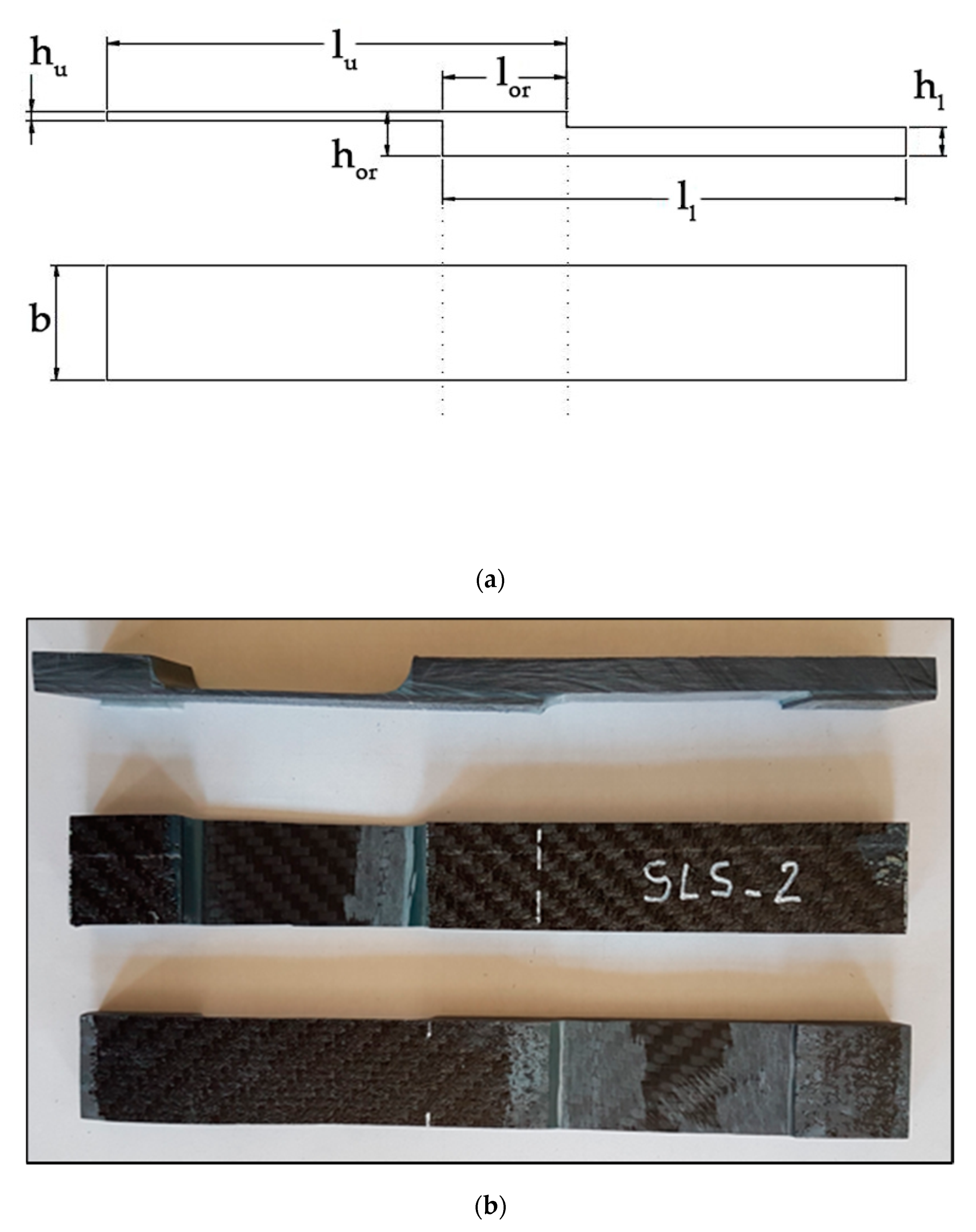
CFRP specimens in the SLS configuration were used in this study. The CFRP prepreg laminates were prepared by impregnating high-strength carbon fibers in the epoxy matrix (SATTI CIT CC206 ER 460). The carbon fibers were woven in the epoxy matrix in a stitched configuration. The laminate plies, which had a nominal thickness of 0.244 mm, were cured using the autoclave method. The upper and lower adherends for the SLS configuration were prepared using the autoclave method. Then, a high-strength epoxy adhesive EA9395, with a shear strength of 25 MPa and a peel strength of 65 MPa, was used for bonding the upper and lower adherends in the SLS configuration. The dimensions of the specimens, the laminate layup configuration, and other dimensional details are presented in Table 1 and Figure 1. A total of three specimens were tested for this research work and were named SLS 1, SLS 2, and SLS 3.
2.2. Experimental Setup
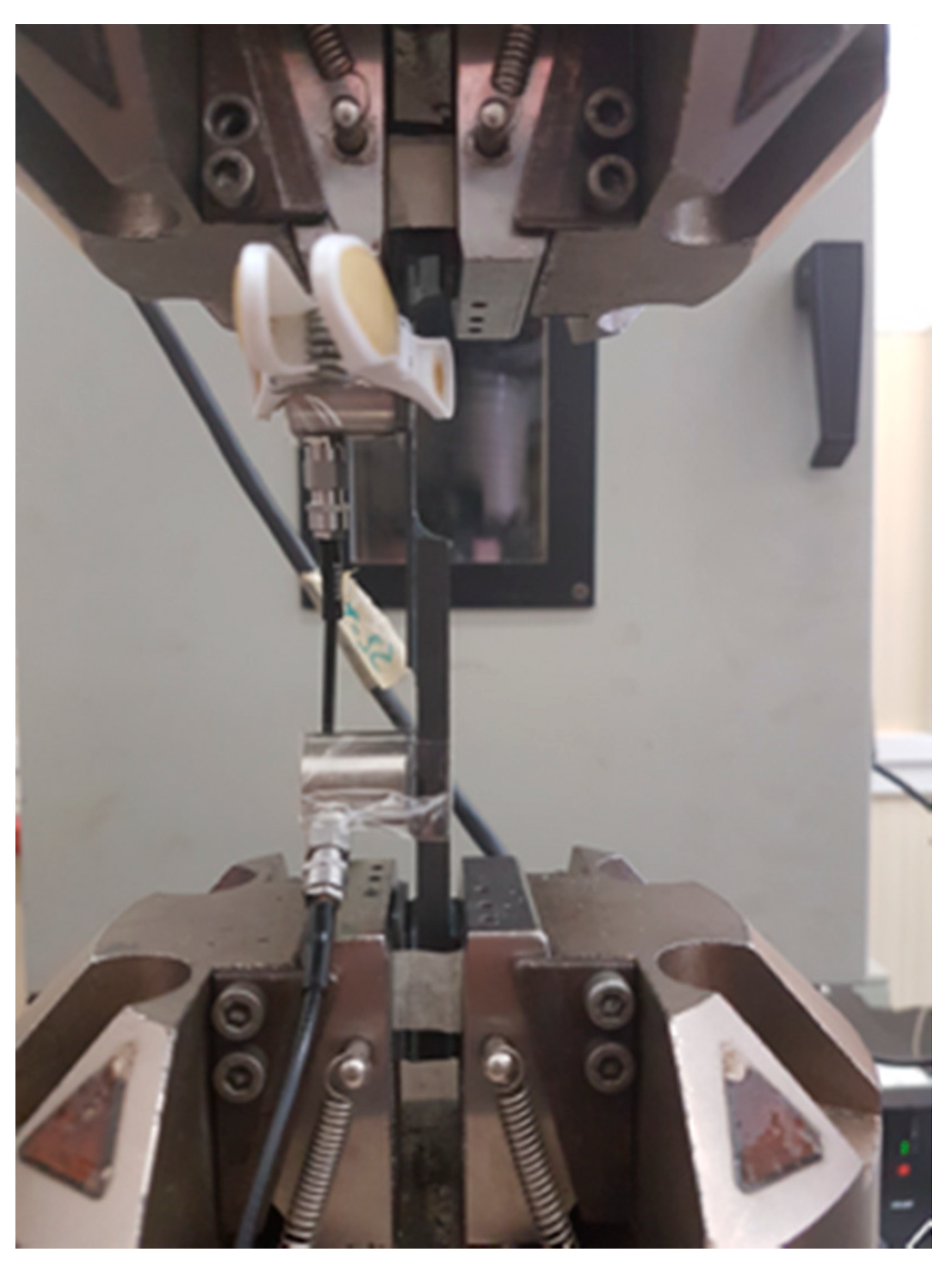
Two narrow-band, general-purpose piezoelectric sensors R-30α (Physical Acoustics, MISTRAS Group, Princeton Jct, NJ, USA) were mounted on the SLS specimens for recording the acoustic signals. The sensors have an operating range of 150 kHz to 400 kHz. The sensors were mounted on the specimens at a distance of 40 mm from the center (Figure 2). The acoustic events generated across this distance, which covered the adhesive overlap region, were recorded for this study. A thin layer of silicone gel separated the piezoelectric transducer surface and the specimen to improve the acoustic coupling and to avoid recording any reverberating signals. All the AE signals were amplified by 40 dB using a 2/4/6 AE pre-amplifier (Physical Acoustics, MISTRAS Group, Princeton Jct, NJ, USA). The acoustic waveforms were recorded at a sampling rate of 1 MSps (1 megasamples per second). The threshold for the acquisition was set as 40 dB.
For the static tensile loading, the ASTM D5868—Standard Test Method for Lap Shear Adhesion for Fiber-Reinforced Plastic Bonding was followed [16]. The static tensile loading was applied in a displacement-controlled mode at a crosshead displacement speed of 13 mm/min. The SLS specimens carried most of the load in the adhesive overlap region in the displacement-controlled testing mode. All the tests were carried out in the INSTRON Servo-Hydraulic testing machine (INSTRON, Norwood, MA, USA), which has a loading capacity of 100 kN.
2.3. Acoustic Emission Features
The acoustic emission descriptors considered for this study are explained in this section. First, the most commonly used parameter, namely, peak amplitude, was used. It represents the largest voltage peak of the recorded AE signal () relative to the reference voltage () set at the pre-amplifier. It is measured in decibels (dB) and it can be expressed as:
Unlike the peak amplitude, which only represents the largest voltage peak, the average signal level (ASL) measures both the negative and positive amplitudes in an acoustic signal with equal weights. In simple words, it provides the average level of the signal in decibels. It can be expressed in volts as:
where is the total number of discretized signal points, is the transient voltage, and is the duration of the signal. The ASL in dB can be expressed as:
The I-Frequency measures the characteristic frequency of the acoustic signal before the peak amplitude is recorded. It is the ratio of the total number of acoustic counts before the peak amplitude (P.Counts) and the duration of the signal for that same instant (Rise time).
R-Frequency is the exact opposite measure of the I-Frequency. It measures the characteristic frequency of the signal after the peak amplitude. It is the ratio of the number of counts after the peak amplitude (Ringdown Counts) and the duration of the signal after that same instance:
A-Frequency is the ratio of the total number of counts recorded above the threshold of acquisition to the duration of the signal:
The peak frequency of an AE signal is the frequency with the largest magnitude when the signal coefficients are analyzed in their frequency domain using a fast Fourier transform (FFT).
These are the parameters that were considered for this study. The method for selecting the best parameters among the aforementioned parameters and the procedure followed for clustering the selected parameters are presented in the next section.
2.4. Methodology for Data Clustering
The different AE features provide the characteristic representation of the acoustic waveform. Many of these AE features are closely related to one another. For example, the absolute energy of the AE signal and the ASL are in direct relationship with the RMS voltage. Absolute energy is directly proportional to the square of the RMS voltage, while ASL is analogous to RMS voltage, with the only difference being that RMS voltage is measured in millivolts or microvolts, whereas ASL is measured in decibels. As such, using both RMS voltage and ASL for analyzing the signal characteristics is redundant.
PCA is a multivariable data reduction technique. The core idea of PCA is to reduce the dimensionally of a dataset that has a large number of interrelated variables, which is essentially the case in this research work. The data reduction is done while retaining as much of the variation present in the dataset as possible. The data reduction is achieved by reducing the data dimensions into new correlated features called principal components, which are minimally correlated.
These principal components form a symmetric matrix, where the eigenvectors of the matrix form the elements of the matrix. These eigenvectors can be defined as the characteristic vectors of the matrix. They are unique in the sense that they remain directionally invariant under linear transformation by its parent matrix. The other details about this analysis can be found in the source article presented by Hotelling [17]. The procedure for calculating the principal components is summarized by Maćkiewicz and Ratajczak [18].
The multiple parameters were reduced using PCA and the characteristic parameters were selected for analysis. Then, these selected parameters were clustered using the fuzzy c-means (FCM) data clustering method. The FCM is a data clustering method for any two-dimensional data. The dataset is clustered into a predefined number of clusters in FCM [19]. Unlike other data clustering methods, in which all the data points belong to only one cluster, in FCM, the data points belong to all the clusters to some degree. The degree of membership is based on the distance between the data point and the centroid of each cluster. The data point has a large degree of membership with the cluster that has the closest centroid, while it has a smaller degree of membership with the cluster that has the farthest centroid.
The assignment of the centroids and the data points to each cluster is determined by the objective function. By iterating, the distance from any given data point to a cluster center is weighted by the membership of that data point in the cluster.
The detailed procedure for performing FCM on a dataset can be found elsewhere. Both the PCA and FCM are popular data analysis methods and their procedures have been described in the literature over the years [17,18,19]. Hence, they are not provided here. Both the FCM and PCA were carried out in MATLAB® -(R2019b); the FCM was supported by the fuzzy logic toolbox in MATLAB® (R2019b).
3. Results and Discussions
The AE data from testing the SLS specimens SLS 1, SLS 2, and SLS 3 were recorded using a pair of piezoelectric sensors. The parameters mentioned in Section 2.3 were derived from the PAC PCI-2 data acquisition system (Physical Acoustics, MISTRAS Group, Princeton Jct, USA).
3.1. PCA for Data Reduction and the Selection of AE Features
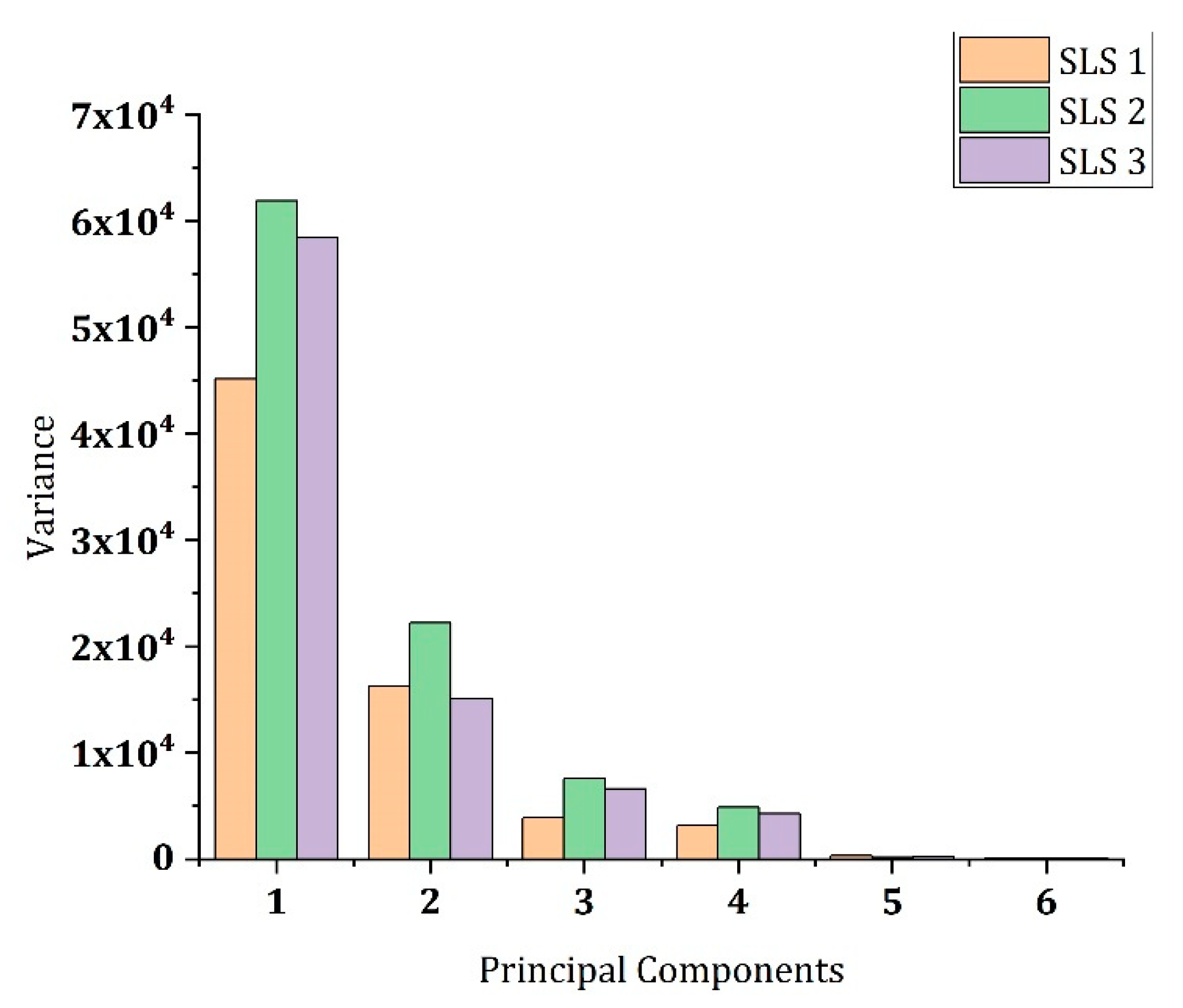
The input parameters of peak amplitude, ASL, I-Frequency, R-Frequency, P-Frequency, and A-Frequency were reduced into their eigenvector matrix using PCA. The variances of the eigenvalues of the eigenvector matrix or the different principal components were also calculated. The scree plots describing the variance of the different principal components are presented in Figure 3. As indicated in the introduction section, the different principal components are the orthogonal linear transformations of the AE data. The set of principal components from 1 to 6 provides a representation of the reduced dataset.
The variances of the first and second principal components were significantly larger than the remaining components combined. Thus, the dataset was reduced to only the first two principal components PC 1 and PC 2.
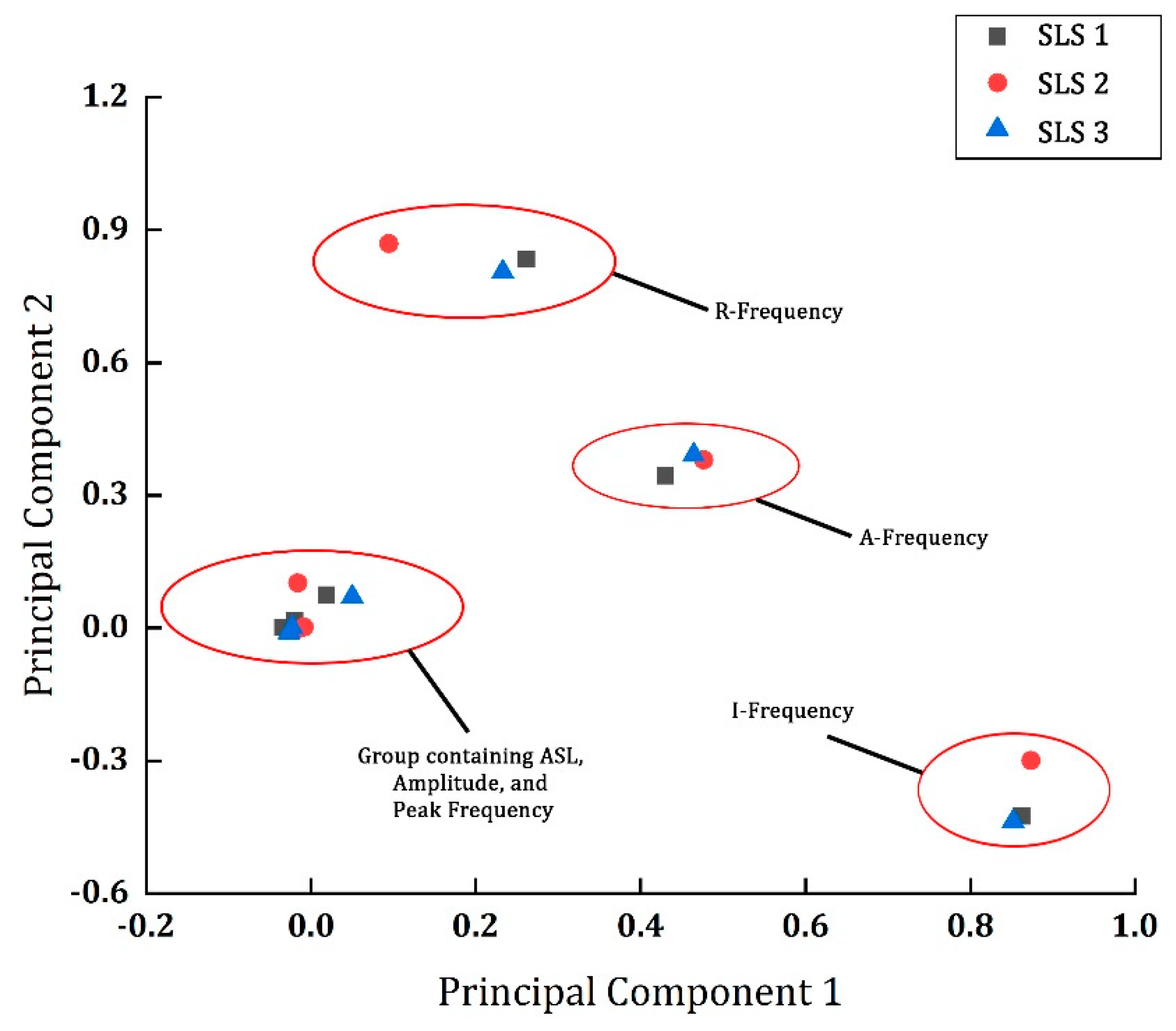
For the reduced data, the eigenvalues of the principal components PC 1 and PC 2 of all the AE parameters are presented in Figure 4. It can be observed that the peak amplitude, peak frequency, and amplitude formed a group with the eigenvalues of PC 1 and PC 2 close to each other. Therefore, a representative AE parameter from this group was selected for further analysis. In this work, the peak amplitude was selected as the representative from the group.
It can also be observed from Figure 4 that the I-Frequency, R-Frequency, and A-Frequency had large variations in their eigenvalues for PC 1 and PC 2 and could not be constituted into a group. This means that there existed a large variation in these parameters. Therefore, the I-Frequency and R-Frequency were considered for the analysis.
From the PCA results, three parameters from the initially assigned group of six parameters were selected: amplitude, I-Frequency, and R-Frequency. Instead of going through a rigorous process of analyzing all the parameters and finding the optimal parameters for analysis, the PCA reduced the dimensionality of the dataset into three parameters. For comparison purposes, the amplitude from the ASL, amplitude, and P-Frequency group was compared with I-Frequency and R-Frequency.
There was a specific reason for comparing the amplitude with these two parameters. For several years in the research of damage assessments using AE, the peak amplitude values were directly related to the damage modes. For instance, the most general trend was that the AE signals with an amplitude above 60–70 dB represent fiber breakage, 35–50 dB represents matrix cracking, and 50–60 dB represents fiber debonding or delamination. There is no definite value for this correlation of the amplitude with damage modes. Different authors use different values based on their experimental results. A summary of this information can be found in the literature [3,20].
In recent years, however, some researchers have argued that the AE signals with high amplitudes not only represent fiber breakage but also interlaminar crack growth [4]. This is because of the mode of propagation and the degree of absorption of the AE waveforms. The peak amplitude only corresponds to the largest voltage peak and the modes of propagation, while the degree of absorption in the propagation medium is ignored. For this reason, the I-Frequency and R-Frequency were considered for this study.
The decaying frequency of the AE signals can be defined using the R-Frequency, while the I-Frequency can define the characteristics of the initiation level before the largest amplitude is recorded. Hence, these two parameters, when compared with the peak amplitude of the signal, can provide information about the acoustic signal characteristics.
3.2. Fuzzy c-Means Data Clustering Results
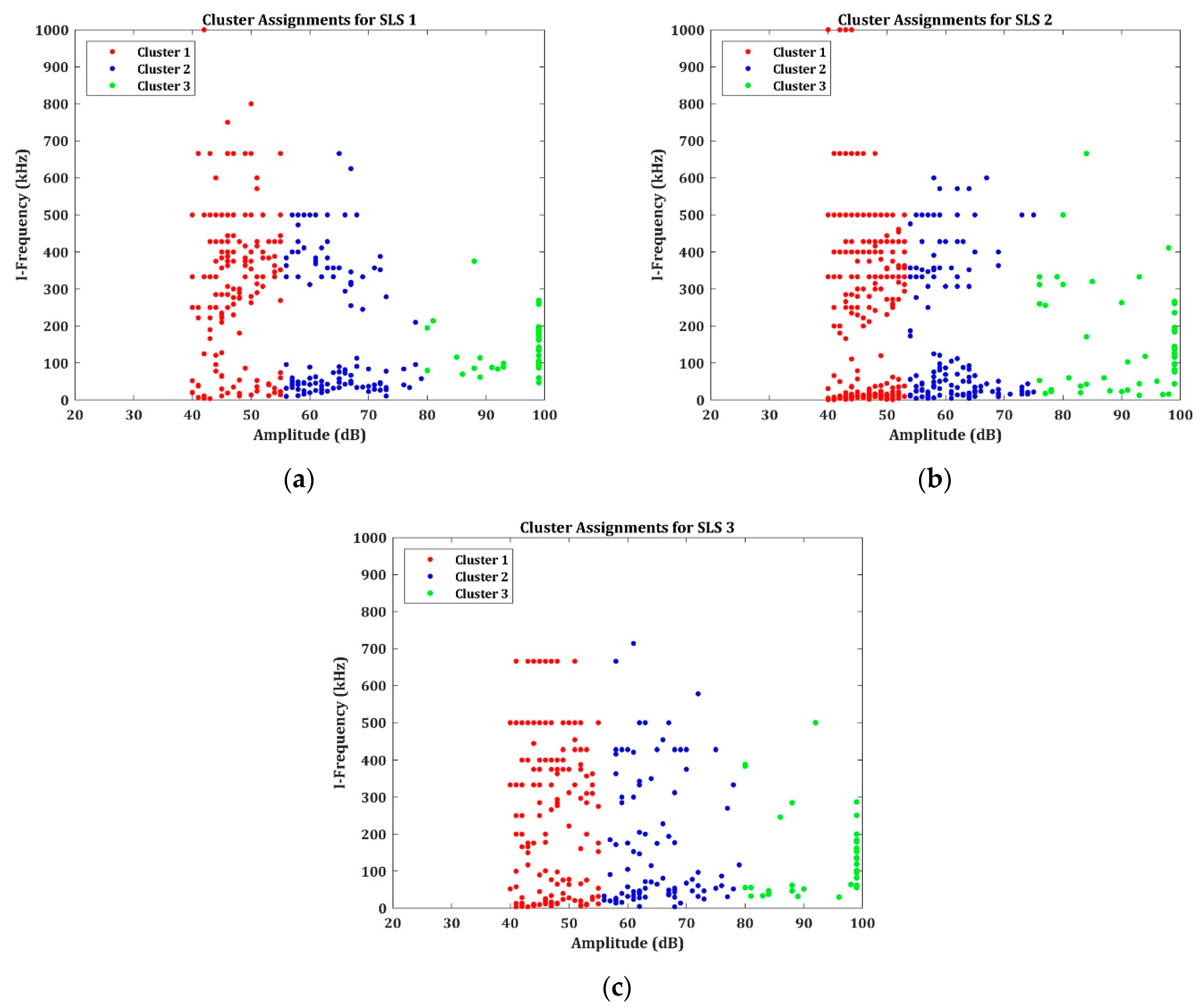
The I-Frequency and R-Frequency with respect to the different amplitudes of the recorded AE events were clustered using the FCM clustering technique. Initially, for selecting the optimal number of clusters, the Davies–Bouldin Index (DBI) was calculated for the abovementioned data. The DBI with the minimum value for the different clusters N = 1, 2, …, 6 is supposed to be selected as the optimal number of clusters. For all sets of data recorded for SLS 1, SLS 2, and SLS 3, the DBI returned the lowest value for N = 3. The FCM was used for clustering I-Frequency and R-Frequency into three clusters. The clustered data of I-Frequency and R-Frequency with respect to amplitude is presented in Figure 5 and Figure 6, respectively, for all SLS specimens.
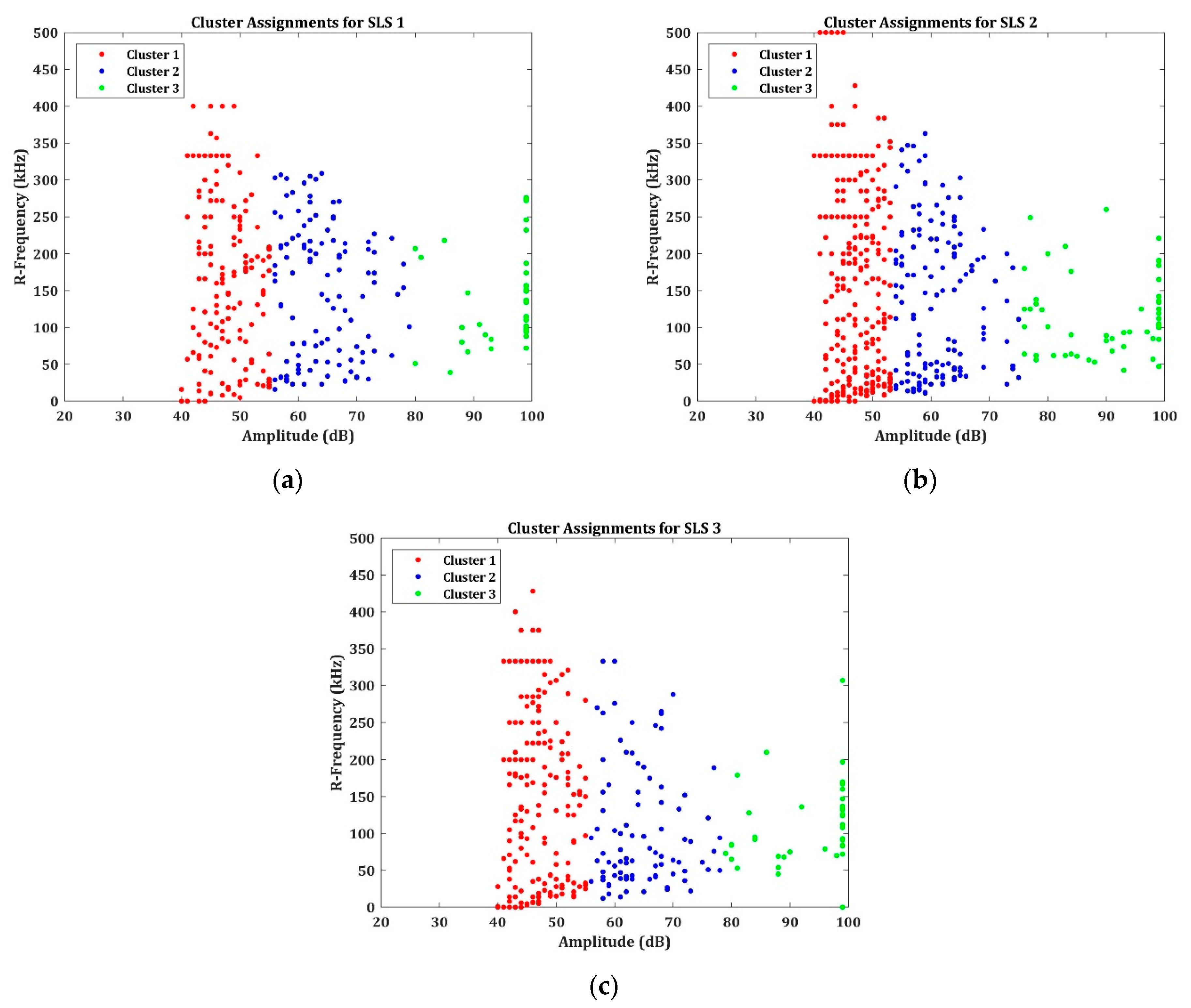
The clustered data in Figure 5 shows that despite the peak amplitude level, the R-frequency of the recorded waveforms varied significantly. Similar results are also observed in Figure 6 for the R-Frequency. Furthermore, the frequency levels for I-Frequency and R-Frequency in Figure 5 and Figure 6 were not very similar for all the AE signals. They differed significantly in several instances. For example, in Figure 5a,b, which shows the I-Frequency of the recorded signals, there were very few AE events recorded between the frequencies of 100 and 200 kHz in cluster 2, and even less AE signals between 100 and 300 kHz below 90 dB in cluster 3. However, in Figure 6a,b, which shows the R-Frequency, the number of AE signals in the frequency range of 100 to 300 kHz was significantly higher. This also meant that the frequency rate of absorption, which can be indicated by the R-Frequency, varied significantly from the I-Frequency. A question may arise: why did the I-Frequency range from 0 to 1000 kHz, while the R-Frequency was only below 500 kHz. The I-Frequency was calculated using Equation (4), which is the ratio of P.Counts to the rise time. If the second or third count of the AE waveform has the largest amplitude, then P.Counts is counted as 1 or 2, respectively. This also means that there was a huge possibility that the rise time could be very short during these instances. By considering the large differences between the short duration of the rise time and the duration of the AE signal, the variation between the I-Frequency and R-Frequency was quite common. This was the reason for the wide range of I-Frequency compared to the R-Frequency.
The I-Frequency clusters can be classified as follows: cluster 1 had AE signals with a low amplitude but with the I-Frequency spread between 0 and 1000 kHz; cluster 2 had AE signals with a moderate amplitude (mostly between 55 and 75/80 dB) with the I-Frequency spread between 0 and 700 kHz; cluster 3 had the signals with higher amplitude (>75/80 dB) but with the I-Frequency spread between 0 and 500 kHz, ignoring the outliers. Since I-Frequency is inversely proportional to the rise time, it can be used as a parameter for classifying the type of damage mode that the AE signals have as their source. Several reports have indicated that the AE signals with a larger peak amplitude and a shorter rise time correspond to an interlaminar crack as the source, while the signals with a smaller peak amplitude and a longer rise time may correspond to the shearing mode under tensile loading. Analogous with these observations, the differences between the shearing mode and the interlaminar crack can be identified [3,5,7]. A detailed explanation of how to identify the damage sources is presented in the next section.
The R-Frequency represents the amount of absorption of the AE signals. The AE signals generally propagate in two different modes: symmetrical and asymmetrical. The symmetrical mode AE signals carry a lower frequency component but have less dispersion in their energy during propagation. The low amount of dispersion means that the R-Frequency can be high for the symmetrical mode. This is because the signal duration in the symmetrical mode of propagation is very low, which leads to the higher R-Frequency. The AE signals generated from matrix cracking and delamination release AE signals, which propagate in symmetric mode. In contrast, the AE signals, which are propagating in asymmetric mode, have a higher frequency and disperse more during propagation. The asymmetric mode AE signals can have a lower R-Frequency compared to the symmetric mode AE signals. These asymmetric AE signals mostly have fiber breakage or interlaminar crack growth as their AE source.
3.3. Damage Assessment Using AE Descriptors
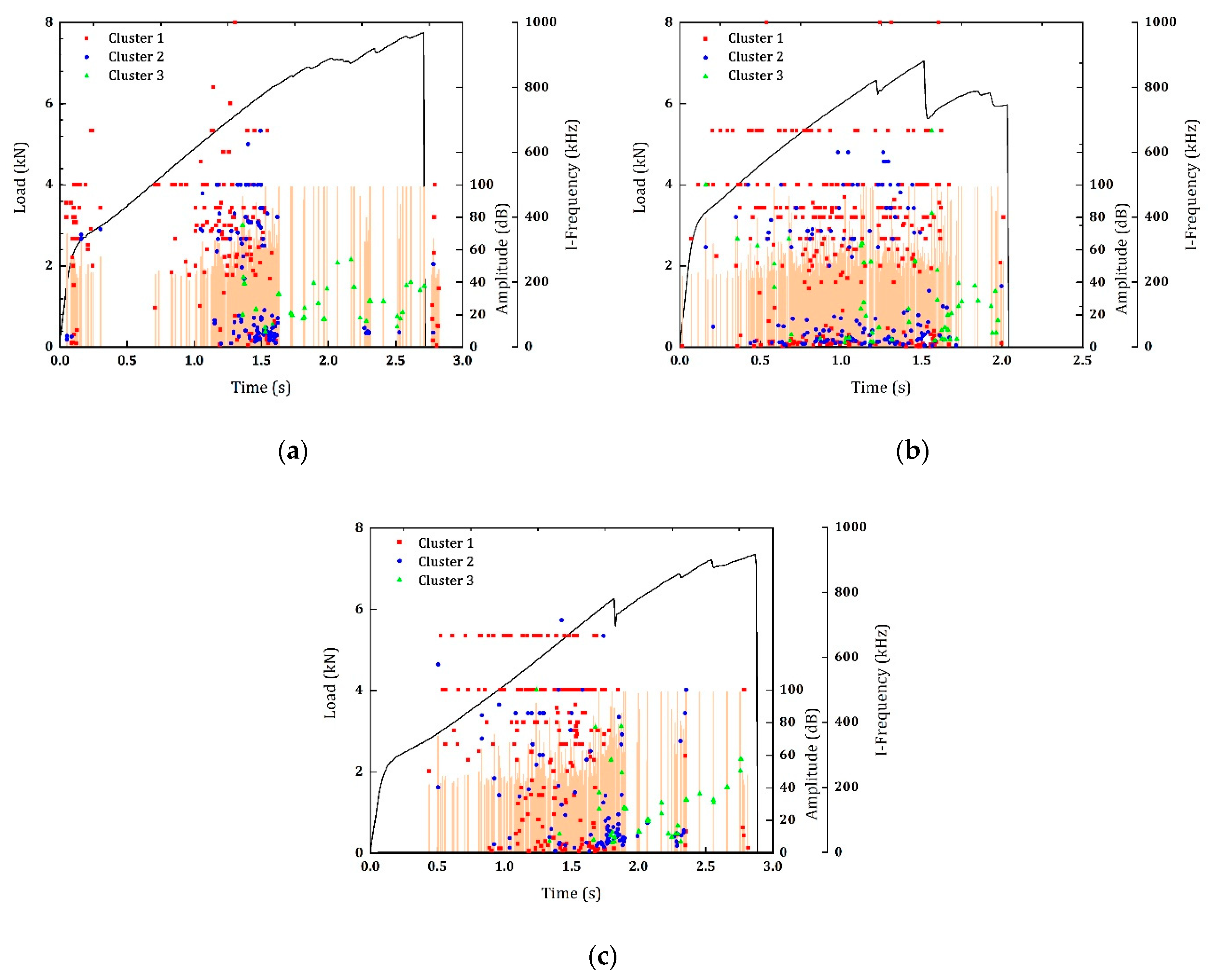
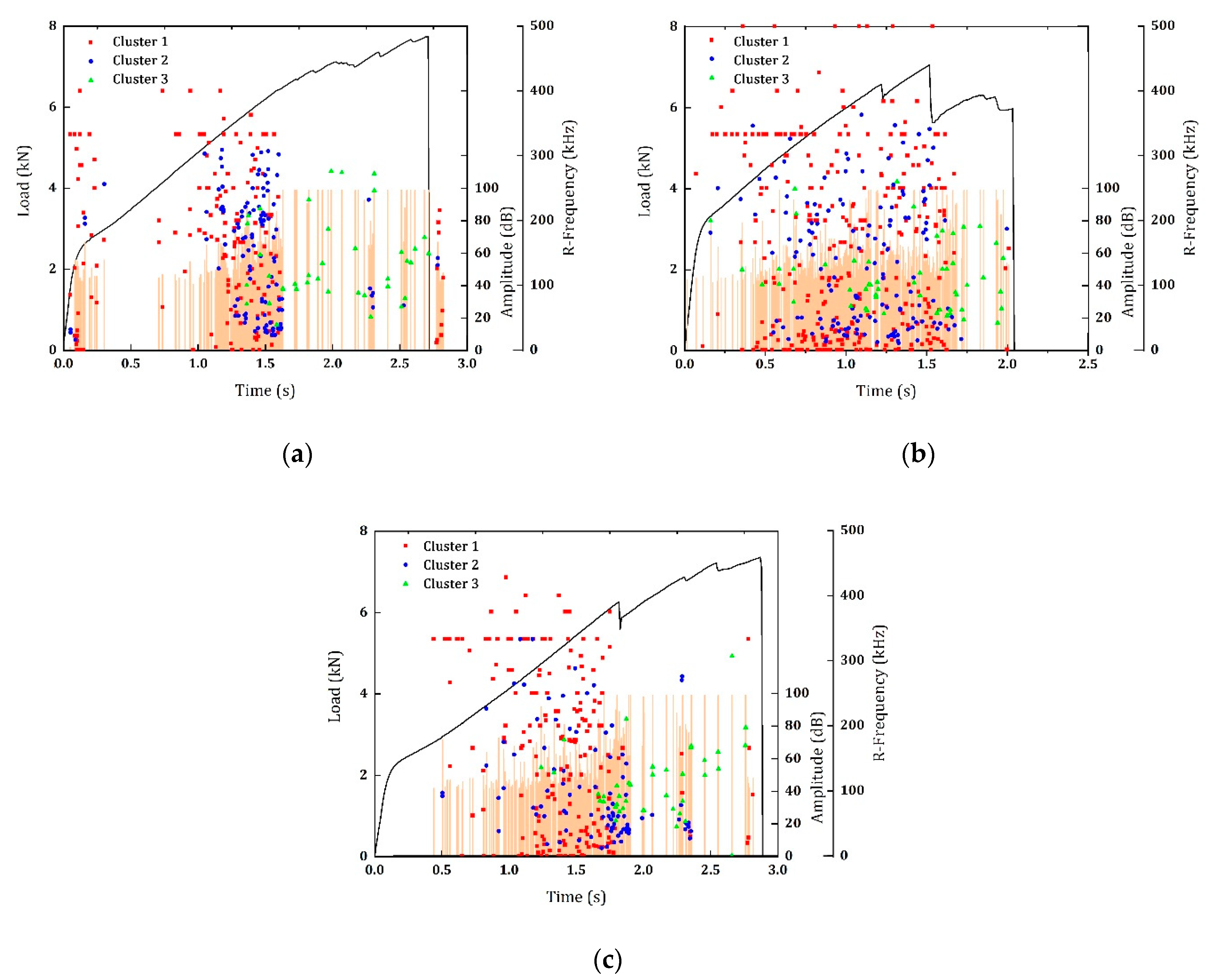
For assessing the damage modes properly, it is essential to map the AE descriptors with the load response of the SLS specimens. The clustered AE data were plotted with respect to the load response of the SLS specimens for detailed analysis. The SLS load response results with I-Frequency and amplitude are presented in Figure 7 and the results with R-Frequency and amplitude are presented in Figure 8.
In Figure 7a, the amplitude and clustered I-Frequency are plotted with respect to the load response of the SLS 1 specimen. First of all, the load responses had multiple load peaks before the final fracture. In our previous works, the authors classified these peaks as regions of initial rupture and final rupture [21]. For SLS 1, the initial rupture occurred at 7.05 kN and the final rupture occurred at 7.75 kN. From the point of initial rupture to the final rupture (roughly between 1.75 s and 2.75 s, the majority of the I-Frequency components were in cluster 3. Comparing this observation with Figure 5a, it can be identified that these clusters belonged to the category of AE signals with a high amplitude and low I-Frequency (<200 kHz). Similarly, if the results are compared with Figure 6a and Figure 8a, again, the AE signals had a low R-Frequency (<200 kHz). This implies that the signals were highly symmetric since both I-Frequency and R-Frequency were below 200 kHz, and at the same time, the peak amplitude was higher. These types of AE signals normally have interlaminar crack growth as their source. If the same figures are compared for the initial stages of load response, say before 0.5 s, the I-Frequency and R-Frequency were highly asymmetric. The signals during this stage were deemed to be asymmetric in the sense that the I-Frequency and R-Frequency varied significantly in the very few AE signals recorded during that short duration. In our previous reports, the authors indicated that this initial loading stage may represent the sliding of the specimen inside the loading grips [21]. The next important stage was the stage between the initial stage and the initial rupture (between 0.75 s and 1.75 s). In Figure 7a, most of the AE signals had I-Frequencies in clusters 1 and 2. A similar observation could be found for R-Frequency in Figure 8a. Owing to the absence of cluster 3 in I-Frequency and R-Frequency, the damage modes in these regions were probably due to the matrix cracking and delamination. It has been indicated by several researchers that in adhesive-bonded components, under static loading conditions, a majority of the load is carried by the adherends [22,23]. The delamination, however, initiated at the vicinity of the adhesive layer and the adherend and extended through the thickness of the adhesive layer. The region before the initial rupture suffered extensive microcracking in the thick adhesive layer and the delamination was initiated. However, the specimen SLS 1 retained its load-carrying capability until it reached 7.75 kN. During this transition stage, the crack had grew through the thickness, releasing AE signals with a high symmetry between I-Frequency and R-Frequency, resulting in the final fracture.
For specimen SLS 2 (Figure 7b and Figure 8b), more than one load peak can be observed. Nonetheless, the major initial rupture occurred at 1.5 s with the load peak of 7.05 kN and the final rupture at 2.25 s at 5.96 kN. It is clear from this observation that the damage modes of SLS 2 were different from those of SLS 1. However, there was an ambiguity in how this damage mode progressed. Comparing these results with the I-Frequency and R-Frequency clusters of Figure 5b and Figure 6b, the cluster 3 signals of I-Frequency and R-Frequency were distributed throughout the loading regions. Between the transition period of the initial and final ruptures, which lasted for only 0.75 s, a significant number of cluster 3 signals were observed. Even though this stage was shorter in duration, these signals still referred to the interlaminar crack growth. The distribution of cluster 3 throughout the loading stages indicates that the crack growth was initiated at a very early stage in SLS 2. This was probably the reason for the very low final rupture load (5.96 kN) compared to the SLS 1 specimen.
The results of the SLS 3 specimens are presented in Figure 7c and Figure 8c, which were almost identical to SLS 1. Interlaminar crack growth was observed between the initial and final rupture stages, which were at 5.93 kN (at 1.75 s) and 7.36 kN (at 2.75 s). The AE signals that corresponded to the matrix cracking and delamination were distributed after the duration of 0.5 s.
The I-Frequency and R-Frequency clustered data can provide information about the damage modes. More detailed analysis, such as counting the number of signals corresponding to matrix cracking and interlaminar crack growth and mapping them with the in-line fractographic analysis can provide detailed information about these parameters.
4. Conclusions
An acoustic emission multiparameter approach was used for identifying the damage modes occurring in CFRP specimens configured in a single-lap shear (SLS) configuration. First, from different AE features, the best features for analysis were selected by reducing their dimensions into principal components using PCA. From the scree plot of the variance for different principal components, it was concluded that the dataset can be reduced to two dimensions. Consequently, from the PCA analysis, the I-Frequency, R-Frequency, and peak amplitudes were chosen to be the best features for analysis. The selected features were clustered using the FCM algorithm into three clusters. Each cluster had I-Frequency and R-Frequency distributed over their peak amplitudes. Then, this clustered information was plotted over the load responses of the SLS specimens for identifying the damage modes. The different damage modes, such as matrix cracking, interlaminar crack growth, and the initial/final stages of rupture were identified by comparing the clustered I-Frequency and R-Frequency of the AE signals plotted over the load responses of the specimens under loading. The future scope of this work is to extend this with an in-line fractographic analysis to directly relate the observed damage modes with the AE features. With this, the AE features can more effectively be used for damage analysis.
Author Contributions
Conceptualization, P.K.V., C.B. and G.P.; methodology, P.K.V.; validation, P.K.V., C.B. and G.P.; formal analysis, P.K.V., C.B. and G.P.; investigation, P.K.V., C.B. and G.P.; data curation, P.K.V. and C.B.; writing—original draft preparation, P.K.V.; writing—review and editing, P.K.V., C.B. and G.P.; supervision, C.B. and C.C.; project administration, C.C. All authors have read and agreed to the published version of the manuscript.
Funding
This research received no external funding.
Institutional Review Board Statement
Not applicable.
Informed Consent Statement
Not applicable.
Data Availability Statement
The data presented in this study are available on request from the corresponding author. The data are not publicly available because it is a part of an extended research campaign.
Conflicts of Interest
The authors declare no conflict of interest.
References
- Giordano, M.; Condelli, L.; Nicolais, L. Acoustic emission wave propagation in a viscoelastic plate. Compos. Sci. Tech. 1999, 59, 1735–1743. [Google Scholar]
- Sause, M.G.R. Acoustic Emission. In In Situ Monitoring of Fiber-Reinforced Composites; Springer: Berlin/Heidelberg, Germany, 2016; Volume 242, p. 131. [Google Scholar]
- Barile, C.; Casavola, C.; Pappalettera, G.; Vimalathithan, P.K. Application of different acoustic emission descriptors in damage assessment of fiber reinforced plastics: A comprehensive review. Eng. Fract. Mech. 2020, 235, 107083. [Google Scholar] [CrossRef]
- Oz, F.E.; Ersoy, N.; Lomov, S.V. Do high frequency acoustic emission events always represent fibre failure in CFRP laminates? Compos. Part. A Appl. S 2017, 103, 230–235. [Google Scholar] [CrossRef]
- Barile, C.; Casavola, C.; Pappalettera, G.; Vimalathithan, P.K. Damage characterization in composite materials using acoustic emission signal-based and parameter-based data. Compos. Part. B Eng. 2019, 178, 107469. [Google Scholar] [CrossRef]
- Barile, C.; Casavola, C.; Pappalettera, G.; Vimalathithan, P.K. Damage assessment of carbon fibre reinforced plastic using acoustic emission technique: Experimental and numerical approach. Struct. Health Monit. 2020. [Google Scholar] [CrossRef]
- Aggelis, D.J.; Barkoula, N.M.; Matikas, T.E.; Paipetis, A.S. Acoustic structural health monitoring of composite materials: Damage identification and evaluation in cross ply laminates using acoustic emission and ultrasonics. Compos. Sci. Technol. 2012, 72, 1127–1133. [Google Scholar] [CrossRef]
- Kharrat, M.; Ramasso, E.; Placet, V.; Boubakar, M.L. A signal processing approach for enhanced Acoustic Emission data analysis in high activity systems: Application to organic matrix composites. Mech. Syst. Signal. Pr. 2016, 70–71, 1038–1055. [Google Scholar] [CrossRef] [Green Version]
- Guel, N.; Hamam, Z.; Godin, N.; Reynaud, P.; Caty, O.; Bouillon, F.; Paillassa, A. Data Merging of AE Sensors with Different Frequency Resolution for the Detection and Identification of Damage in Oxide-Based Ceramic Matrix Composites. Materials 2020, 13, 4691. [Google Scholar] [CrossRef] [PubMed]
- Soden, P.D.; Hinton, M.J.; Kaddour, A.S. Biaxial test results for strength and deformation of a range of E-glass and carbon fibre reinforced composite laminates: Failure exercise benchmark data. Compos. Sci. Technol. 2002, 62, 1489–1514. [Google Scholar] [CrossRef]
- Hinton, M.J.; Kaddour, A.S.; Soden, P.D. Evaluation of failure prediction in composite laminates: Background to “part B” of the exercise. Compos. Sci. Technol. 2002, 62, 1481–1488. [Google Scholar] [CrossRef]
- Hinton, M.J.; Soden, P.D. Predicting failure in composite laminates: The background to the exercise. Compos. Sci. Technol. 1998, 58, 1001–1010. [Google Scholar] [CrossRef]
- Liptai, R.G.; Harris, D.O.; Tatro, C.A. (Eds.) An introduction to acoustic emission. In Acoustic Emission; ASTM International: West Conshohocken, PA, USA, 1972; pp. 3–10. [Google Scholar]
- Liptai, R.G. Acoustic emission from composite materials. In Composite Materials: Testing and Design; Corten, H., Ed.; ASTM International: West Conshohocken, PA, USA, 1972; pp. 285–298. [Google Scholar]
- Hamstad, M.A. Thirty years of advances and some remaining challenges in the application of acoustic emission to composite materials. In Acoustic Emission—Beyond the Millennium; Kishi, T., Ohtsu, M., Yuyama, S., Eds.; Elsevier: Oxford, UK, 2000; pp. 77–91. [Google Scholar]
- ASTM D5868-01(2014). Standard Test Method for Lap Shear Adhesion for Fiber Reinforced Plastic (FRP) 361 Bonding; ASTM International: West Conshohocken, PA, USA, 2014. [Google Scholar]
- Hotelling, H. Analysis of a complex of statistical variables into principal components. J. Educ. Psychol. 1933, 24, 417. [Google Scholar] [CrossRef]
- Maćkiewicz, A.; Ratajczak, W. Principal Component Analysis. Comput. Geosci. 1993, 19, 303–342. [Google Scholar] [CrossRef]
- Fotouhi, M.; Sadeghi, S.; Jalalvand, M.; Ahmadi, M. Analysis of the damage mechanisms in mixed-mode delamination of laminated composites using acoustic emission data clustering. J. Therm. Compos. Mater. 2017, 30, 318–340. [Google Scholar] [CrossRef] [Green Version]
- Chandarana, N.; Sanchez, D.M.; Soutis, C.; Gresil, M. Early Damage Detection in Composites during Fabrication and Mechanical Testing. Materials 2017, 10, 685. [Google Scholar] [CrossRef] [PubMed]
- Barile, C.; Casavola, C.; Moramarco, V.; Pappalettere, C.; Vimalathithan, P.K. Bonding Characteristics of Single- and Joggled-Lap CFRP Specimens: Mechanical and Acoustic Investigations. Appl. Sci. 2020, 10, 1782. [Google Scholar] [CrossRef] [Green Version]
- Roderick, G.L.; Everett, R.A.; Crews, J.H. Debond propagation in composite-reinforced metals. In Fatigue of Composite Materials; ASTM International: West Conshohocken, PA, USA, 1975. [Google Scholar]
- Mangalgiri, P.D.; Johnson, W.S.; Everett, R.A., Jr. Effect of adherend thickness and mixed mode loading on debond growth in adhesively bonded composite joints. J. Adhes. 1987, 23, 263–288. [Google Scholar] [CrossRef]
Figure 1.
(a) Schematic configuration of a single-lap shear (SLS) specimen and (b) SLS specimens prepared using the autoclave method.
Figure 1.
(a) Schematic configuration of a single-lap shear (SLS) specimen and (b) SLS specimens prepared using the autoclave method.

Figure 2.
Experimental setup with AE sensors mounted on the specimen.

Figure 3.
Scree plot for the different principal components for SLS 1, SLS 2, and SLS 3.

Figure 4.
Principal components PC 1 and PC 2 for all the parameters selected for all specimens.

Figure 5.
I-Frequency vs. amplitude plotted as three clusters using FCM for the (a) SLS 1, (b) SLS 2, and (c) SLS 3 specimens.
Figure 5.
I-Frequency vs. amplitude plotted as three clusters using FCM for the (a) SLS 1, (b) SLS 2, and (c) SLS 3 specimens.

Figure 6.
R-Frequency vs. amplitude plotted as three clusters using FCM for the (a) SLS 1, (b) SLS 2, and (c) SLS 3 specimens.
Figure 6.
R-Frequency vs. amplitude plotted as three clusters using FCM for the (a) SLS 1, (b) SLS 2, and (c) SLS 3 specimens.

Figure 7.
Load, amplitude, and clustered I-Frequency vs. time for the (a) SLS 1, (b) SLS 2, and (c) SLS 3 specimens.
Figure 7.
Load, amplitude, and clustered I-Frequency vs. time for the (a) SLS 1, (b) SLS 2, and (c) SLS 3 specimens.

Figure 8.
Load, amplitude, and clustered R-Frequency vs. time for the (a) SLS 1, (b) SLS 2, and (c) SLS 3 specimens.
Figure 8.
Load, amplitude, and clustered R-Frequency vs. time for the (a) SLS 1, (b) SLS 2, and (c) SLS 3 specimens.


Table 1.
SLS specimen nomenclature, geometry, and configurations.
| Upper Adherend | ||||
| Length lu (mm) | Width bu (mm) | Thickness hu (mm) | No. of Plies | Stacking Sequence |
| 101.6 ± 0.11 | 25.33 ± 0.12 | 1.3 ± 0.05 | 5 | +45/+45/+45/−45/+45 |
| Lower Adherend | ||||
| Length ll (mm) | Width bl (mm) | Thickness hl (mm) | No. of Plies | Stacking Sequence |
| 101.6 ± 0.09 | 25.33 ± 0.14 | 6.4 ± 0.12 | 26 | +45/[+45/−45]12/+45 |
| Overlapping Region | ||||
| Length lor (mm) | Width bor (mm) | Thickness hor (mm) | ||
| 26 ± 0.12 | 25.33 ± 0.25 | 8.5 ± 0.11 | ||
Publisher’s Note: MDPI stays neutral with regard to jurisdictional claims in published maps and institutional affiliations. |
© 2021 by the authors. Licensee MDPI, Basel, Switzerland. This article is an open access article distributed under the terms and conditions of the Creative Commons Attribution (CC BY) license (http://creativecommons.org/licenses/by/4.0/).
Share and Cite
MDPI and ACS Style
Barile, C.; Casavola, C.; Pappalettera, G.; Vimalathithan, P.K. Multiparameter Approach for Damage Propagation Analysis in Fiber-Reinforced Polymer Composites. Appl. Sci. 2021, 11, 393. https://doi.org/10.3390/app11010393
AMA Style
Barile C, Casavola C, Pappalettera G, Vimalathithan PK. Multiparameter Approach for Damage Propagation Analysis in Fiber-Reinforced Polymer Composites. Applied Sciences. 2021; 11(1):393. https://doi.org/10.3390/app11010393
Chicago/Turabian StyleBarile, Claudia, Caterina Casavola, Giovanni Pappalettera, and Paramsamy Kannan Vimalathithan. 2021. "Multiparameter Approach for Damage Propagation Analysis in Fiber-Reinforced Polymer Composites" Applied Sciences 11, no. 1: 393. https://doi.org/10.3390/app11010393
Note that from the first issue of 2016, this journal uses article numbers instead of page numbers. See further details here.