Application of Predictive Maintenance Concepts Using Artificial Intelligence Tools


Faculty of Engineering, University of Porto, 4200-465 Porto, Portugal
*
Author to whom correspondence should be addressed.
Appl. Sci. 2021, 11(1), 18; https://doi.org/10.3390/app11010018
Submission received: 19 November 2020
/
Revised: 16 December 2020
/
Accepted: 18 December 2020
/
Published: 22 December 2020
(This article belongs to the Special Issue Systems Engineering: Availability and Reliability)
Abstract
:The growing competitiveness of the market, coupled with the increase in automation driven with the advent of Industry 4.0, highlights the importance of maintenance within organizations. At the same time, the amount of data capable of being extracted from industrial systems has increased exponentially due to the proliferation of sensors, transmission devices and data storage via Internet of Things. These data, when processed and analyzed, can provide valuable information and knowledge about the equipment, allowing a move towards predictive maintenance. Maintenance is fundamental to a company’s competitiveness, since actions taken at this level have a direct impact on aspects such as cost and quality of products. Hence, equipment failures need to be identified and resolved. Artificial Intelligence tools, in particular Machine Learning, exhibit enormous potential in the analysis of large amounts of data, now readily available, thus aiming to improve the availability of systems, reducing maintenance costs, and increasing operational performance and support in decision making. In this dissertation, Artificial Intelligence tools, more specifically Machine Learning, are applied to a set of data made available online and the specifics of this implementation are analyzed as well as the definition of methodologies, in order to provide information and tools to the maintenance area.
1. Introduction
Maintenance is a relevant factor for the competitiveness of an organization, since the actions carried out at this level have a direct impact on aspects such as the cost, deadlines and quality of the products produced or services provided [1,2]. Maintenance is a support to the operational area of a company and cannot be dissociated from it, given the implication it has in terms of the efficiency of productive assets. These two areas, operation and maintenance, must operate in parallel in order to guarantee the availability and the rapid response of human and material resources to operational problems, thus ensuring the achievement of objectives with the maximization of available resources. Thus, it becomes important not only to achieve the proposed objectives, but also to achieve them with the minimum consumption or use of resources [2].
It is in this context of constant transformation that Industry 4.0 arises [1]. Industry 4.0 implements the tools provided by advances in information and communication technologies in order to increase the levels of automation and digitalization in industrial and production processes [1,3]. The objective is to manage the entire value chain process, improving production efficiency and creating superior products and services. One of the key points of this technological evolution is the data, which is now more easily read, processed, stored, analyzed and shared between machines and human beings [4]. Additionally, the Internet of Things (IoT) is defined as an ecosystem in which the objects and equipment inserted in it are equipped with sensors and other digital devices, thus being able to gather and exchange information with each other, in a networked system [1].
In recent years, a drop in cost and an increase in the reliability of sensors, data transmission and storage devices have promoted the emergence of condition monitoring systems for industrial equipment. Simultaneously, the IoT allows real-time transmission of this information about the conditions of the systems captured by different monitoring devices. This development offers an excellent opportunity to use condition monitoring data intelligently within predictive maintenance, combining the ability to collect data with an effective and integrated analysis of it [5].
In this sense, the potential of Artificial Intelligence tools, more specifically Machine Learning, allows us to aim for an improvement in the availability of systems, reducing maintenance costs, increasing operational performance and safety, and the ability to support decision making in relation to the ideal time and the ideal action for carrying out the maintenance intervention [4,5,6,7].
Machine Learning can be defined as “the field of study that gives the computer the ability to learn without being explicitly programmed”. It can be said that “Machine Learning algorithms use computational methods to learn information directly from data without using predefined equations as a model” [8].
The main objective of this work is to apply Artificial Intelligence tools, more specifically Machine Learning, to a set of data, coming from different sources, available online [9]. Furthermore, we seek to analyze the specificities of this implementation and the definition of methodologies, in order to provide information and tools to the maintenance area.
2. Machine Learning Process Workflow and Techniques
One of the main difficulties of applying a Machine Learning process to maintenance data is the choice of the right workflow, as in literature there are many different approaches to this problem, depending on the origin of the data and the objectives of the analysis [10,11,12,13]. As the different applications are difficult to compare, in this work it was decided to explore a simple but complete framework and to use a set of data that can be used by other researchers, as the data set is publicly available.
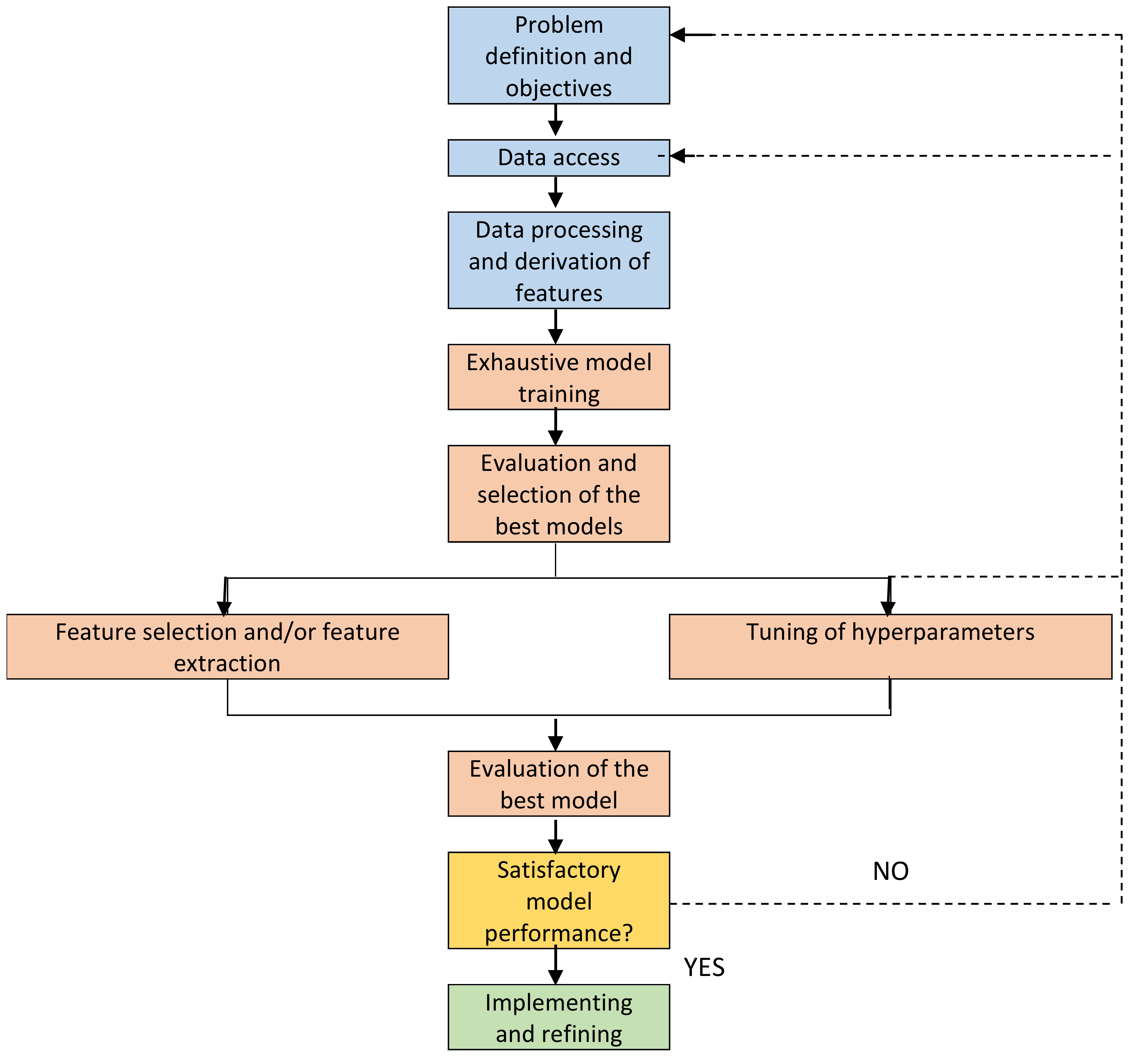
In the present work, the workflow presented in [14], represented in Figure 1, will be followed. From our point of view, a Machine Learning project must always start with the establishment of rigorous and clear definition of the objectives, since such a system fulfills a very specific task and the definition of vague objectives can mean that the model developed is not able to predict exactly what it is intended to.
Quite possibly, the most important part of a Machine Learning project is the ability to understand the data used and how it relates to the task we want to solve. It will not be effective to randomly choose an algorithm, use the data set we have available and expect good results [15]. It is necessary to understand what is happening in the data set before starting to build a model. When building a Machine Learning solution, we must answer or at least keep in mind the following questions: What questions are we trying to answer? Does the available data set allow you to answer these questions? What is the best way to paraphrase my question as a Machine Learning problem? Is the available data set sufficient to represent the problem we are trying to solve? What features (or attributes) have been extracted and will they be able to lead to the correct predictions? How to measure the success of the application of Machine Learning? How will the Machine Learning solution interact with the rest of the process?
Machine Learning algorithms and methods are only part of a larger process for solving a specific problem, and it is important to keep that in mind. Sometimes, a lot of time is spent building complex Machine Learning solutions, only to discover in the end that they do not solve the problem that we were waiting for [16]. By deepening the technical aspects of Machine Learning, it is easy to lose sight of the final goals. It is important to keep in mind all the assumptions created, either explicitly or implicitly, when building Machine Learning models.
Typical machine learning algorithms, such as the hidden Markov models [17], hidden semi-Markov models [18], self-organizing neural network [19], SVM [20], multimodal deep support vector classification [21], deep random forest [22], genetic algorithms [23], blind source separation [24], fuzzy logic [25], k-nearest neighbor algorithms [26] and Bayesian algorithms [27], etc., have been applied in fault diagnosis of dynamic equipment. To the best of our knowledge, there are two main categories of approach for fault diagnosis of gearboxes: Data-driven and physical model-based methods. Although these methods have been successfully applied in many applications, it is very difficult to know what is the best algorithm to apply to a particular data set.
A systematic review of the scientific literature was carried out in [28], from which it is possible to draw several conclusions. Predictive maintenance strategies are being applied to the most diverse equipment, in multiple areas. The equipment where these methods are applied include, but are not limited to, turbines, engines, compressors, pumps. About 89% of the published papers use a set of real data, with 11% using synthetic data. Regarding the use of Machine Learning algorithms in scientific publications, the most used is Random Forest (RF)—33%, followed by methods based on Neural Networks (NN), such as Artificial NN, Convolution NN, Long Short-Term Memory Metwork (LSTM) and Deep Learning—27%, Support Vector Machine (SVM)—25% and k-means—13%. There was also a greater tendency to use vibration signals.
3. Application Example
3.1. Data Applied
Throughout this paragraph, the process of implementing Machine Learning algorithms to a set of maintenance data will be detailed and explained.
First, the data set is presented and the choice is justified. Then, the objectives of this Machine Learning application are rigorously and clearly established. Subsequently, the data set is processed through feature engineering, creating new features in order to seek better performance from the models. The data set used is key to solving Machine Learning problems. A sensible choice of what data to use and how to handle it is crucial to improving the performance of the algorithms. According to Domingos [29], feature engineering is the key to Machine Learning projects and that, often, the measured signals are not suitable for the learning process, and it is necessary to build features from those that are.
Then, the data set is divided into training, validation and testing subsets and the first application of Machine Learning models was carried out, where a variety of algorithms were trained and evaluated. The training process of the algorithms is carried out in the training subset and the validation subset provides an impartial assessment of the fit of the models to the training data, while simultaneously fine-tuning the model and its hyper-parameters in order to seek better performance. Finally, the test set is used to obtain an estimate of the model’s performance, simulating its behavior for future data.
3.2. Data Sources
Despite the growth of this area, due to business competitiveness, sharing sensitive information of this nature is rare, which means that the number of publicly available datasets (relevant to this application) is very scarce.
Within an industrial environment, there is a very complete data set, made available by Microsoft, published in [9], of relevance to the present project.
This dataset contains data from five different sources:
- real-time telemetry;
- error log;
- maintenance history;
- fault history; and
- information about machines
The data were acquired over a year (2015) for one hundred machines, except for the maintenance history, which also contains records for the year 2014.
For a total of one hundred machines, from four different models, the data set contains 876,100 hourly telemetry records, that is, 8761 records per machine. The failure records contain 3919 entries and the maintenance history 3286. The failure history has 761 records, that is, on average, about 8 failure records per machine, throughout 2015. Each machine has 4 components of interest for analysis and also 4 sensors, which measure tension, pressure, vibration and rotation. A controller monitors the system and is able to alert you to the occurrence of 5 types of errors.
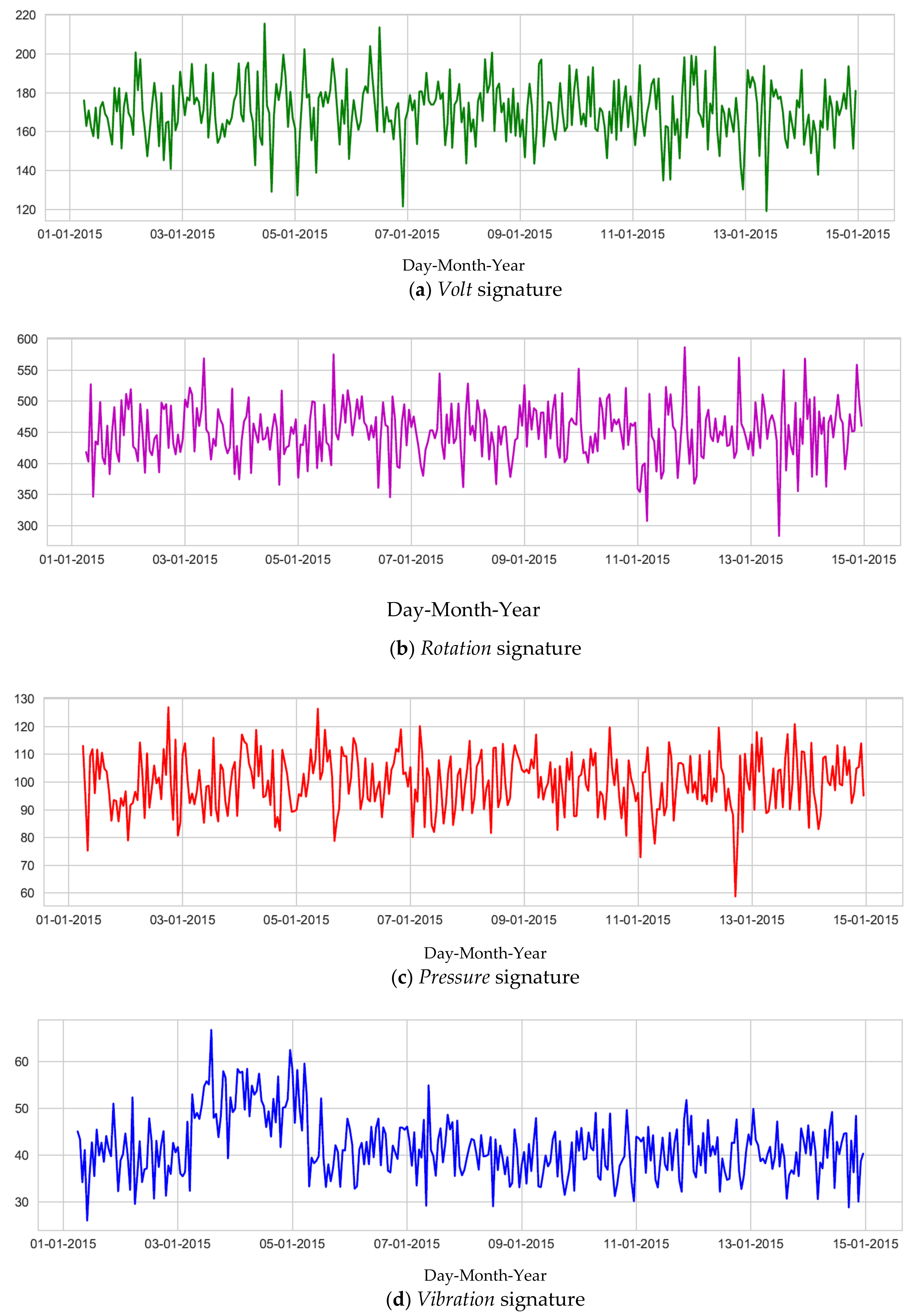
Thus, real-time telemetry data consists of measurements from different sensors (4 per machine), with the associated date and time. The measurements of voltage (“volt”), rotation (“rotate”), pressure (“pressure”) and vibration (“vibration”) are acquired in real time and the average of these measurements over an hour is recorded in Table 1.
To better understand the behavior of each sensor, a simple statistical analysis is performed in Table 2, where the mean, the standard deviation, and the minimum and maximum values are calculated for the parameters voltage (“volt”), rotation (“rotate”), pressure (“pressure”) and vibration (“vibration”) during 2015. As an example, Figure 2 shows the graphical evolutions of the Tension signals (Figure 2a), Rotation (Figure 2b), Pressure (Figure 2c) and Vibration (Figure 2d), over the first fifteen days of January 2015, for machine 1 (machineID = 1).
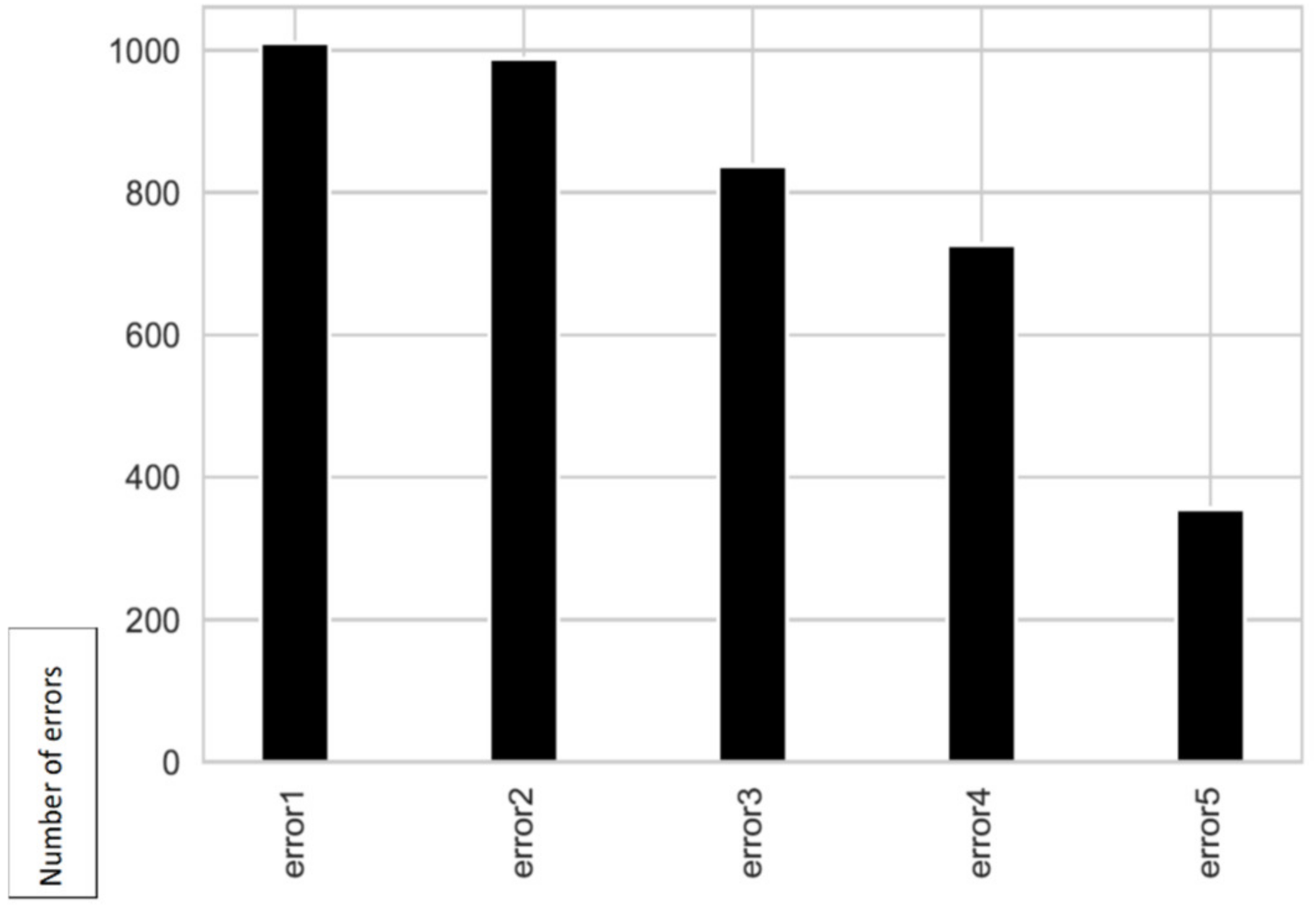
The second source of information is the error log. These are errors that did not immediately lead to a failure, as the machine remained operational. There are 5 types of errors: error1, error2, error3, error4, error5. The date and time are rounded to the nearest time. Each record consists of a date/time, machine and type of error—Table 3. The total number of error records over the year 2015 is 3919. In Figure 3 it is possible to observe the number of errors per type over the year 2015.
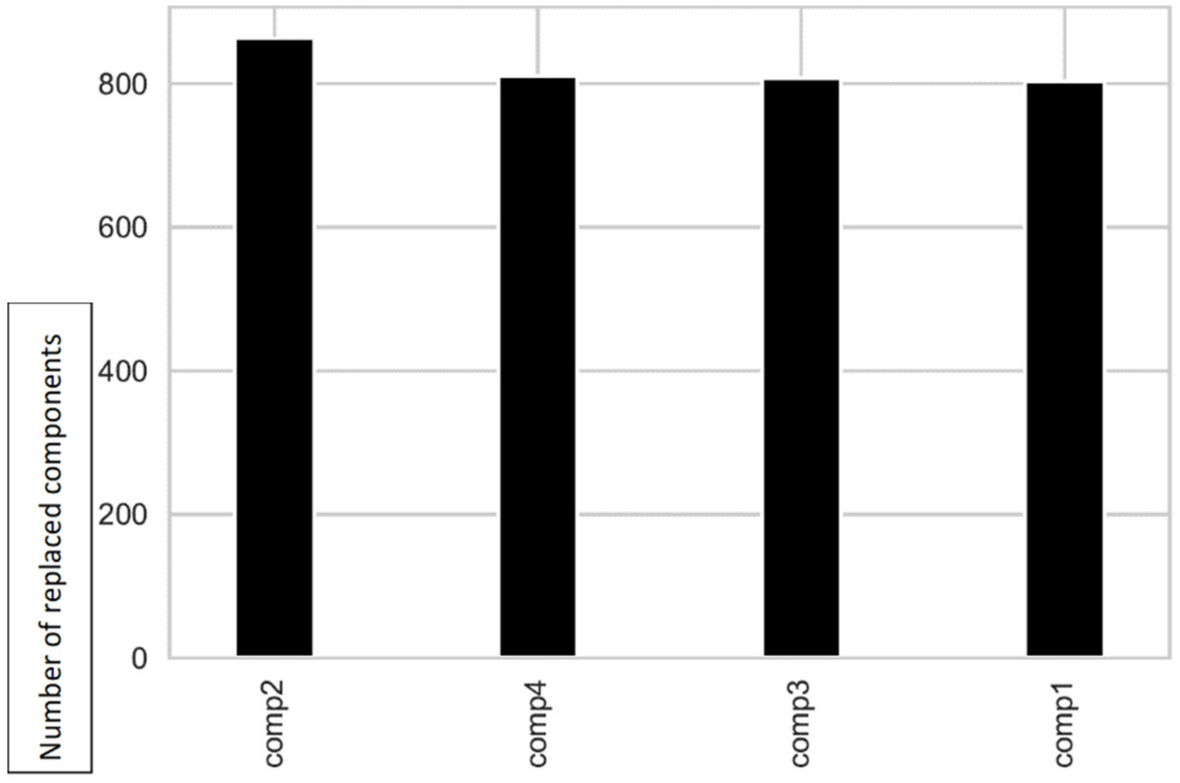
The maintenance records contain data of component replacements resulting from a scheduled or unscheduled maintenance intervention, periodic inspections, or performance degradation. In case of maintenance intervention due to the failure of a component, a fault record is also generated, see next paragraph. For each machine, this data set contains information about 4 types of components: comp1, comp2, comp3, comp4. The date and time are rounded to the nearest time. Each record consists of a date/time, machine and the type of component replaced—Table 4. The total number of maintenance records throughout 2015 is 3286. As previously mentioned, the maintenance records also contain entries for 2014. Figure 4 shows the number of components replaced, by type. It is possible to observe that in this case the number of substitutions is similar for the 4 types of components.
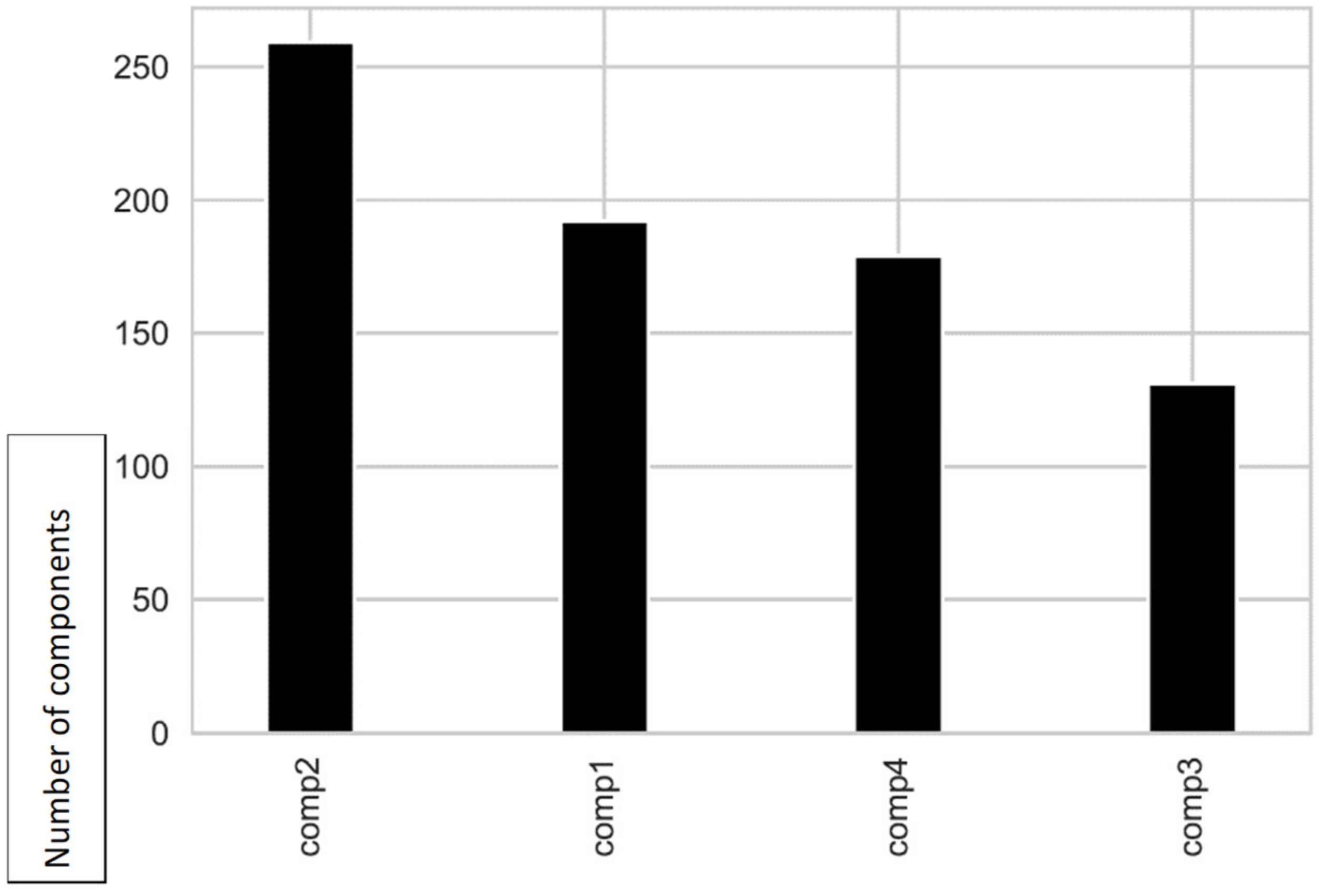
The fault records contain the component replacement records, resulting from the maintenance intervention, due to the occurrence of a fault. The data is for the 4 types of components: comp1, comp2, comp3, comp4. The date and time are rounded to the nearest time. Each record consists of a date/time, machine and the type of replaced component—Table 5. The total number of failure records during 2015 is 761. In Figure 5, it is possible to observe the number of replacements, by type of component, during 2015, due to the occurrence of a failure.
3.3. Definition of Objectives
As already mentioned, a Machine Learning project must start with the rigorous and clear establishment of objectives. In this case, the main objective of the models used will be to predict the probability of a failure occurring within the defined time window. More specifically, the probability of a machine failure occurring in the next 24 h (duration of the time window chosen for this application) related to one of the components (components 1, 2, 3 or 4).
Then, given that a particular and clear objective has already been set, more specific questions can be asked about Machine Learning itself: (1) Should supervised, unsupervised, or reinforcement learning models be chosen or, possibly, combinations of learning modes? (2) Whether supervised learning, classification, or regression? (3) Are models intended to train immediately as new data is obtained (batch learning or online learning)?
After analyzing the problem, and bearing in mind the proposed objective, we opted for supervised learning and, in particular, classification. Furthermore, taking into account the existence of 4 different components under analysis, the problem will be multi-class classification (“Multiclass Classification”). It was also considered that it will not be necessary, given the scope of the problem and the nature of the data, for models to train immediately as new data is obtained. Therefore, we are facing a problem of batch learning.
3.4. Feature Engineering
A feature is a predictive attribute for the model. The purpose of feature engineering is to seek to increase the predictive power of Machine Learning algorithms, creating new features from the available data. As a rule, feature engineering is carried out in the first place and then the selection of features occurs, eliminating irrelevant, redundant or highly correlated features. Starting from the different sources of information presented in the previous paragraphs, a single dataset will be created, which will be used for the application of predictive models.
The historical data that models have access to are individual moments in the past. In particular, for telemetry data, disturbances resulting from measurements, such as noise, are possible, thus making the predictive task more difficult. In this way, the data can be aggregated in time windows, thus allowing to “smooth” the values, minimizing the effects of noise on the features used by the models.
Bearing in mind how far in the future the model should be able to predict, according to the requirements of the project, it is important to define how far it should “look” to make these predictions. This interval of time passed to where the model should “look back” is called lag. Several features can be extracted from these time intervals—lag features. The data set used to generate lag features usually has a date/time associated with it.
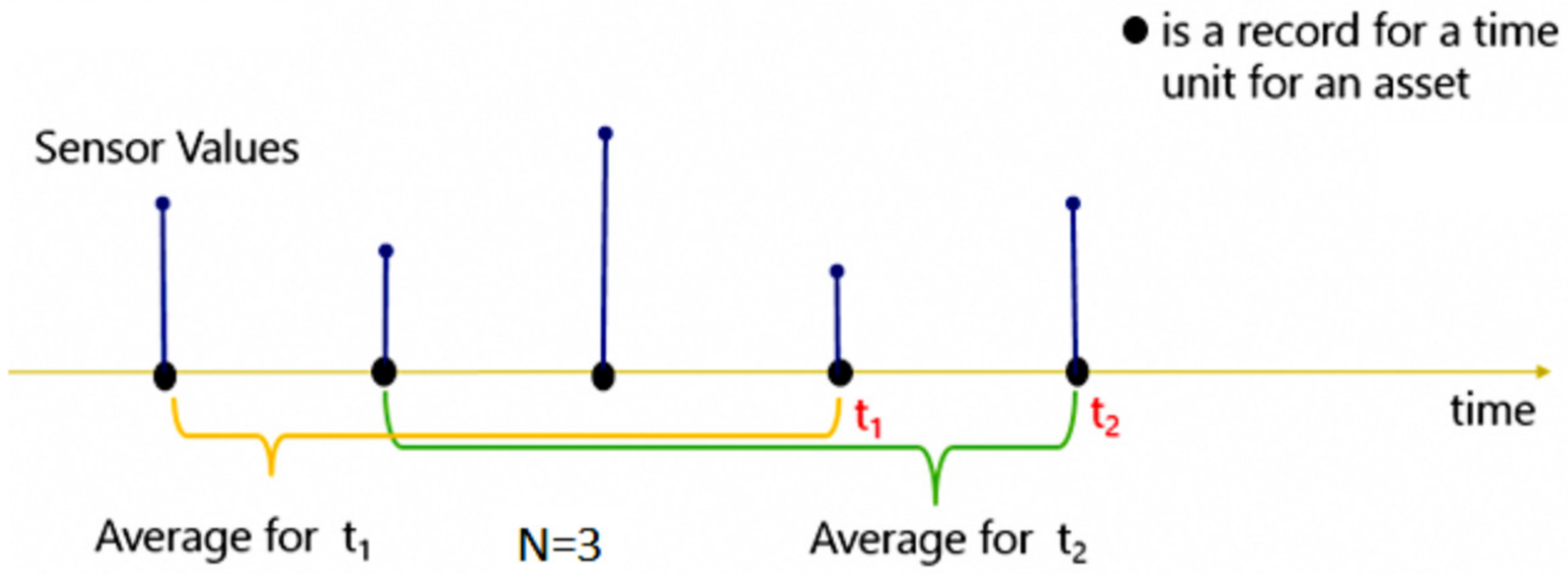
For each record, a time window of dimension N is created and the lag features are calculated for the period N before the date/time of that record. Figure 7 shows an example of this application for a ti measurement with N = 3. The value of N is typically in minutes or hours, depending on the nature of the data.
Thus, two temporal windows were created. The first, of 3 h, in order to allow us to portray the behavior of telemetry data in the short term (Table 7) and the second, of 24 h, in order to represent the long-term evolution (Table 8). In each of these time intervals, two new parameters were calculated every 3 h for each of the features: the moving average and the standard deviation. Note that, in the case of N = 24 h (Table 8), naturally the two new parameters are not available for the initial moments (first 24 h).
As with telemetry data, the error log also has a date/time associated with it. However, these data are categorical and not numerical. In this case, the number of errors of each type is added, every 3 h, for the time window N = 24 (Table 9). Each line in the table represents the sum of the number of errors of each type in the 24 h prior to the indicated datetime.
The maintenance log, which contains information related to the replacement of components, allows the generation of new potentially important features, such as, for example, how long ago a component was last replaced—Table 10. It is expected that this feature relates well to the possible failures of the components, since, the longer the time of use of a component, the greater the expected degradation.
It is relevant to note that the creation of features based on maintenance data is not as linear as in the previous cases. However, this type of case-specific feature engineering is very common in predictive maintenance, where domain knowledge and experience play a crucial role in understanding and creating relevant features.
Finally, information about the machines can be used without further modifications, that is, information related to the model and number of years in service of each machine—Table 6.
3.5. Feature Selection
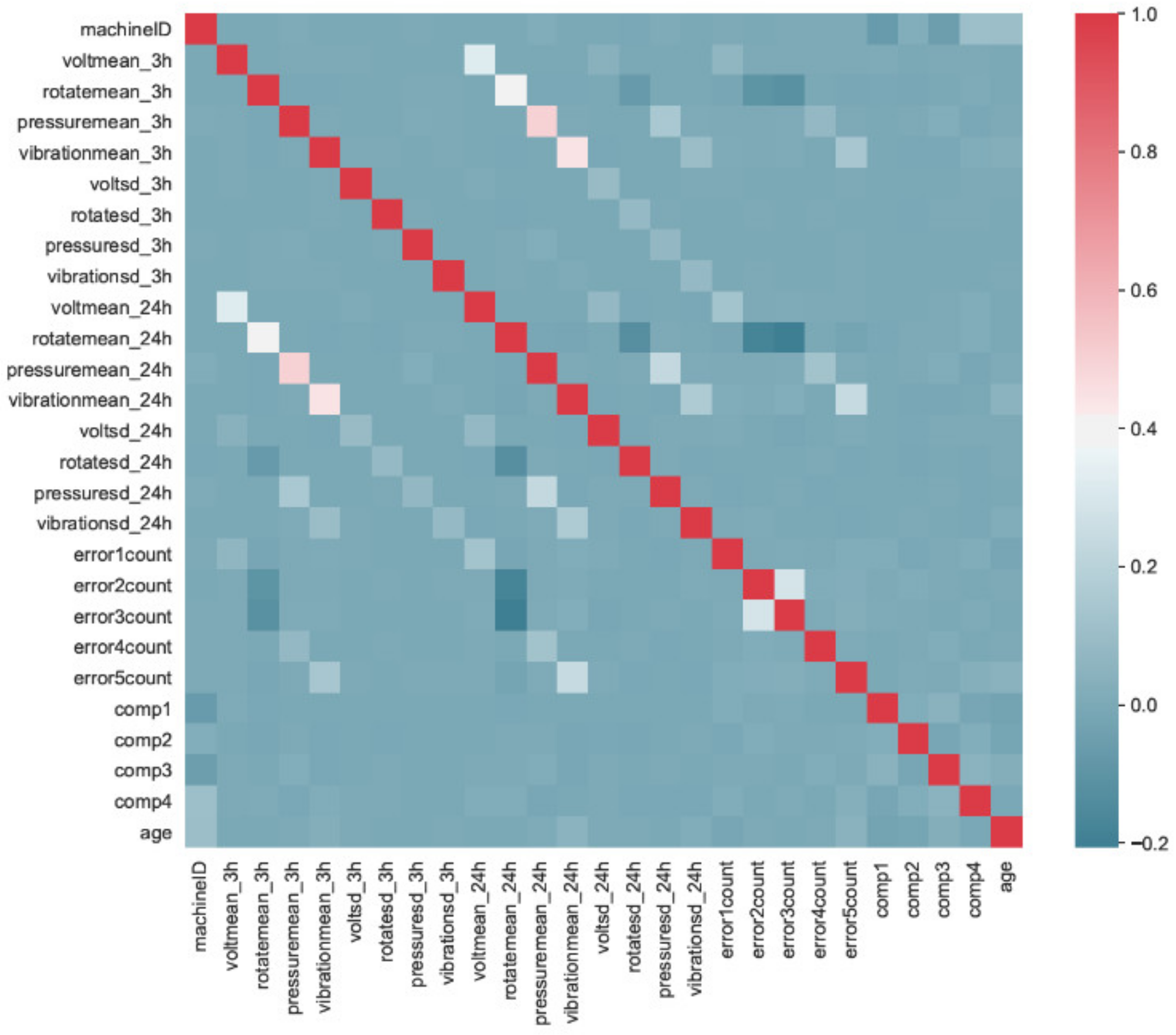
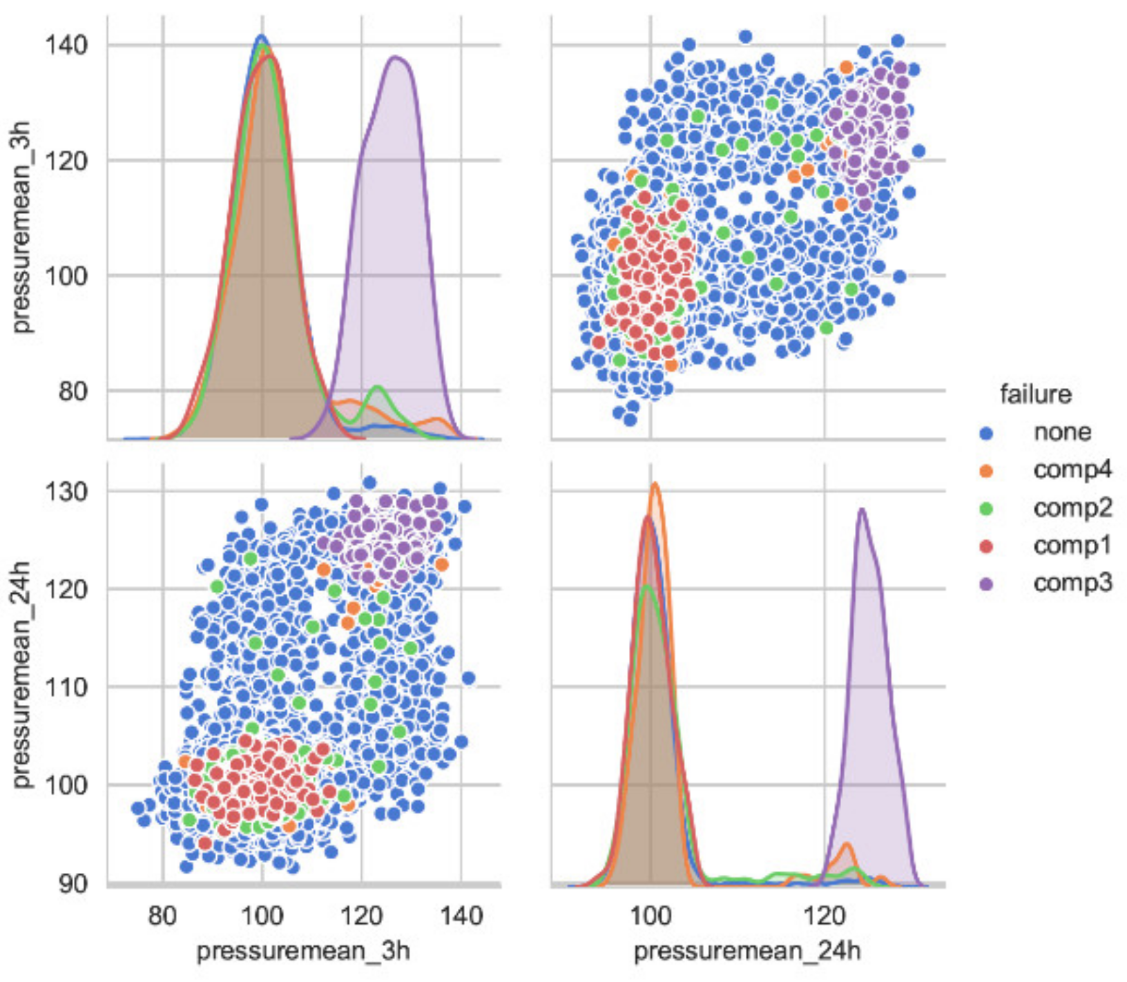
An analysis of the linear correlation between the variables was performed (Figure 8). The correlation coefficient varies between −1 and 1. This coefficient makes it possible to see whether one variable justifies the linear variation of another. When it is close to 1, it means that there is a strong positive correlation, that is, if a given feature A increases, then feature B also increases and if A decreases, B it also decreases.
In this case, it appears that the correlation between the features is mostly low or nonexistent (correlation coefficient close to zero). Even so, in the case of the features pressuremean_3h and pressuremean_24h, the value of the correlation coefficient is approximately 0.5 and a more detailed analysis will be relevant.
Thus, Figure 9 shows the failures, by type of components, according to the evolution of the features pressuremean_3h and pressuremean_24h. It is possible to observe that, for components 1 and 3, there are clusters of points.
However, the same is not true for components 2 and 4. It is likewise possible to observe that most failures for component 3 occur for higher pressuremean_3h and pressuremean_24h values, when compared with the other components. Thus, it was decided to keep both features, since there is a clear relationship between these and the occurrence of failures in at least some of the components
3.6. Classification of Data and Construction of Labels
As previously mentioned, the problem of predictive maintenance under analysis is a case of Supervised Learning. In order to train a model to predict failures, it is necessary for not only examples of failure but also a time series of observations that led to that failure. Furthermore, the model needs examples of “normal” operating periods in order to be able to see the difference between the two. The classification between these two states is binary (stable or without failure/unstable or with failure). With this information available (stable/unstable), the model is only useful if it is able to promptly alert you to the imminence of a failure.
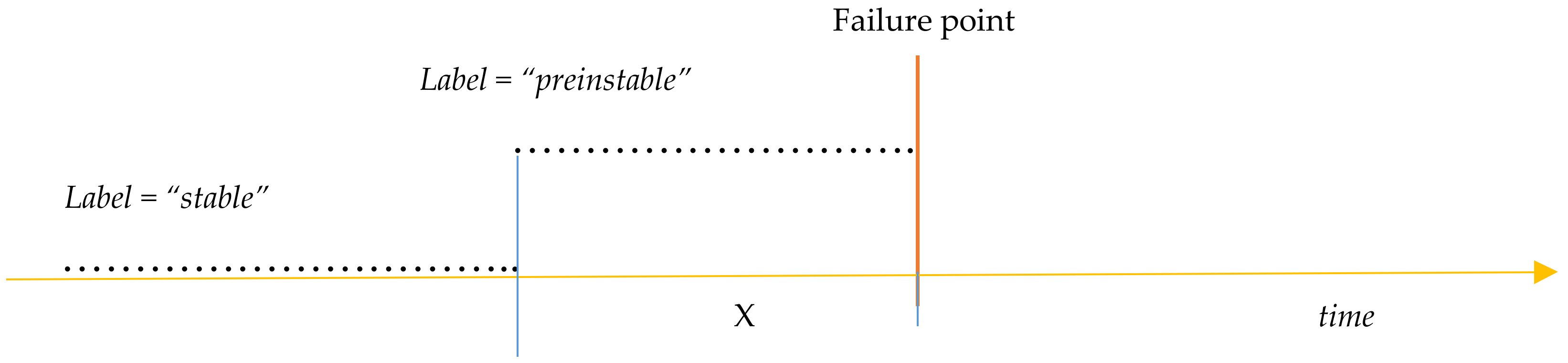
In order to fulfill this early warning criterion, it is necessary to modify the definition of the failure event label, which occurs at a specific time, to a time interval where the failure event may occur. The time until the failure occurs, which delimits the boundary between the two categories, must be chosen according to operational criteria. Is the knowledge that a failure will occur within 12 h sufficient to prevent it? And what about 24 h? And two weeks? The model’s ability to predict a failure will also depend on the duration of this time window.
This process is illustrated in Figure 10. In order to achieve the reset from unstable to pre-unstable, observations within the time window (represented by “X” in Figure 9) before the occurrence of a failure have been labeled as pre-instable, while records outside this time interval X have been labeled as stable.
The main objective of the Machine Learning models used will be to predict the probability of a failure occurring within this time window. In this case, more specifically, the probability of a machine failure occurring in the next 24 h (duration of the time window chosen for this application) related to one of the components (components 1,2,3 or 4). Thus, a new categorical feature “failure” was created, where all records in the 24 h prior to the occurrence of a failure in component 1 have the value failure = comp1 and so on for components 2,3 and 4. Records that do not check these conditions have the value of failure = none. This leads to the problem turning from a binary problem (stable/pre-unstable) to a multi-class classification problem (stable/n pre-unstable component). It should also be noted that, henceforth, due to this redefinition of failure event, when it is mentioned that a certain algorithm predicts a failure, in fact, what is being mentioned is that the algorithm predicts the occurrence of a failure within this time window.
Table 11 shows examples of failure in component 2. Note that the first 8 records occur in the 24 h prior to the occurrence of the first failure of component 2. The next 8 records in the 24 h prior to another failure of component 2.
3.7. Data Splitting
When working with associated day and time data, as is the case here, the division between the training, validation and test sets must be carried out carefully, in order to ensure that the evaluations obtained correspond to the actual performance that should be expected of the models, since there is an inherent temporal correlation between observations (high similarity between temporally close data). This validation technique is called Holdout.
In problems of predictive maintenance, in most situations, the best option is to perform a division based on time, that is, choose a point in time, train the model with all records prior to that point, using the later records to validate the model. This methodology also allows to simulate how the model will actually behave in practice.
Thus, in the present application, the registrations until 08/31/2015 1:00:00 were assigned to the test set, the registrations between 01/09/2015 1:00:00 and 31/10/2015 1:00:00 to the validation set and registration from 01-11-2015 1:00:00 to the test set. In order to guarantee that the data in different sets do not share time windows, the records at the borders, that is, the records of the 24 h preceding the date of division, have been removed. Thus, Table 12 shows the amount of data that was attributed to each of the sets and the percentage that corresponds to failures.
3.8. Class Imbalance in Maintenance Problem Applications
Something to take into account in predictive maintenance is the fact that the occurrence of failures is rare during the life cycle of a given machine, when compared to normal operation. This leads to an imbalance between classes (Table 13), which usually leads to an illusory performance on the part of the algorithms, which tend to classify the most common example more often at the expense of the less common, since the total number of incorrect classifications are thus less. Therefore, the Recall and Precision values can be low, although the Accuracy value is high. A clear example of this phenomenon is, in the validation set (where most of the evaluation metrics will be calculated), where 98.11% (Table 12) of the data correspond to the Stable category (failure = none), that is, a model (without any use) that provides functioning stable values at all times would have an Accuracy of 98.11%. It is therefore essential to look at other evaluation metrics.
For a considerable number of critical equipment applications, the model’s inability to predict a failure can be exorbitantly expensive. In predictive maintenance, as a general rule, the most important is the number of real failures that the model is capable of predicting, that is, the model’s Recall3. This parameter becomes even more important as the consequences of false negatives, that is, true failures that the model was unable to predict, exceed the consequences of false positives, that is, a false prediction of a failure. This phenomenon is known as “incorrect classification cost” and can be estimated by companies according to the cost of repair, parts and labor. Generally, it is preferable that the model errs as a precaution, since it will be more economical to carry out a maintenance check than a partial or total interruption of the operation. However, the wrong prediction of a failure, that is, a false positive, can also lead to a loss of time and resources. In this case, the model must be adjusted to a high Precision. However, as mentioned earlier, the Recall and Precision metrics are not independent: Increasing one implies decreasing the other.
3.9. Application of Models in the Validation Set
In this first application, the validation set is used in order to understand how a wide variety of models behave, as well as to look for the tuning of the hyper-parameters of certain models. Such an approach is due to the fact that it is not possible, at the outset, to determine which algorithm is most suitable for a given problem. When training and evaluating a wide variety of models at an early stage, it is possible to see which ones have the greatest potential, however, for this step to be successful, it is necessary that the metrics for evaluating the models have been chosen in accordance with the established objectives.
The models tested were K-Nearest Neighbors, Decision Tree, Random Forest, Naïve Bayes and Artificial Neural Networks. The best results were obtained by Random Forest and Artificial Neural Networks models [32].
3.10. Test Set Behavior
The validation set has been used, so far, to fine-tune the models and respective hyper-parameters, in order to seek better performance. It is now important to check how the models behave in the test set. Although, in a real case, it is advisable to evaluate only the model that is intended to be implemented [8], this section presents the results obtained for the evaluation of the two best models (in the validation set), in this case, Random Forest and Artificial Neural Networks, with min-max scaling normalization.
Table 14 and Table 15 show the values obtained for Precision, Recall and F1 Score, for the Random Forest and Artificial Neural Network model, respectively, in the validation and test sets.
As expected, there is a generalized decrease in performance of the evaluation metrics in the test set. Still, the results remain satisfactory. As previously mentioned, in predictive maintenance, as a general rule, the most important is the number of real failures that the model is capable of predicting, that is, the value of the model’s Recall parameter [28]. This parameter becomes even more important as the consequences of false negatives, that is, true failures that the model was unable to predict, exceed the consequences of false positives, that is, a false prediction of a failure [33,34].
For both models, there is a drop in the value of Recall (and, consequently, of F1Score) to values below 90% for component 1 in the test set. In the present application, the four components were considered to be of equal importance.
In a real application, where it may be possible to know more information about each one of them (such as cost, importance in the process, location in the equipment, ease of replacement), the analysis may involve trying to optimize certain metrics that are considered to be of greater relevance.
4. Conclusions
In this paper, Machine Learning models were applied to a dataset available online. The data set used was published by Microsoft, in [9], in a Notebook for Predictive Maintenance and Machine Learning. The use of this data set was justified. In the implementation carried out in the present project, until the final phase of feature engineering, the steps presented in that Notebook were followed. However, from that moment on, as it is considered that the approach presented in [9] is too simplistic (no validation technique is used and only a single model is applied), it was decided to deepen the analysis with the implementation of the Holdout validation, which divides the data set into three subsets (Training, Validation and Test), as well as various Machine Learning models, thus showing how to fine-tune the models and respective hyper-parameters using the validation set.
The fact that it is a multi-class classification problem added complexity to the analysis and, perhaps, starting with a binary classification problem may be advisable for a better understanding of the basic concepts of Machine Learning, fundamental to the success of any application.
It is possible to address the imbalance between classes, very common in maintenance applications, since the occurrence of failures is rare during the life cycle of a given machine, when compared to its normal operation.
At the outset, and knowing that a sensible choice of which data to use and how to handle it is crucial for the performance of Machine Learning algorithms, good results would be expected based on the result obtained. However, more important than any result was the demonstration of a methodology, starting from data of different types and sources (very common in maintenance applications), that allowed us to show how it is possible to visualize and treat them in order to apply Artificial Intelligence tools in the analysis of maintenance data, in this case, Machine Learning.
Although the results obtained compare well with those presented so far in the literature, the biggest disadvantage in using the presented methodology lies in the definition of the features. If the selection of features is not the most correct, the results obtained can lead to wrong predictions. For future work, the application of feature learning concepts will be considered instead of feature engineering, which appears to be promising to improve the results obtained [35,36].
Author Contributions
D.C.: developed and performed the work during is M.Sc. thesis; L.F.: supervised the work and prepared and edited the manuscript. All authors have read and agreed to the published version of the manuscript.
Funding
This research received no external funding.
Conflicts of Interest
The authors declare no conflict of interest.
References
- Gilchrist, A. Industry 4.0: The Industrial Internet of Things; Springer: Berlin/Heidelberg, Germany, 2016; ISBN 978-1-4842-2047-4. [Google Scholar]
- Kobbacy, K.A.H.; Murthy, D.N.P. (Eds.) Complex System Maintenance Handbook; Springer Science & Business Media: Berlin/Heidelberg, Germany, 2008; ISBN 978-1849967006. [Google Scholar]
- Kagermann, H.; Lukas, W.-D.; Wahlster, W. Securing the Future of German Manufacturing Industry Recommendations for Implementing the Strategic Initiative INDUSTRIE 4.0; Final report of the Industrie 4.0 Working Group; Acatech-National Academy of Science and Engineering: Frankfurt, Germany, 2013. [Google Scholar]
- Ribau, J. Afinal, o que é isto da Indústria 4.0? Available online: https://visao.sapo (accessed on 7 June 2020). (In Portuguese).
- Paolanti, M.; Romeo, L.; Felicetti, A.; Mancini, A.; Frontoni, E.; Loncarski, J. Machine learning approach for predictive maintenance in industry 4.0. In Proceedings of the 14th IEEE/ASME International Conference on Mechatronic and Embedded Systems and Applications (MESA), Oulu, Finland, 2–4 July 2018; pp. 1–6. [Google Scholar]
- Li, Y.; Wang, K. Modified convolutional neural network with global average pooling for intelligent fault diagnosis of industrial gearbox. Eksploat. Niezawodn. Maint. Reliab. 2020, 22, 63–72. [Google Scholar] [CrossRef]
- Rodrigues, J.; Costa, I.; Torres Farinha, J.; Mendes, M.; Margalho, L. Predicting motor oil condition using artificial neural networks and principal component analysis. Eksploat. Niezawodn. Maint. Reliab. 2020, 22, 440–448. [Google Scholar] [CrossRef]
- Müller, A.C.; Guido, S. Introduction to Machine Learning with Python: A Guide for Data Scientists; O’Reilly Media Inc.: Sebastopol, CA, USA, 2016; ISBN 1449369901. [Google Scholar]
- Microsoft. Predictive Maintenance Modelling Guide. 2018. Available online: https://notebooks.azure.com/Microsoft/projects/PredictiveMaintenance (accessed on 1 May 2020).
- Çınar, Z.M.; Abdussalam Nuhu, A.; Zeeshan, Q.; Korhan, O.; Asmael, M.; Safaei, B. Machine Learning in Predictive Maintenance towards Sustainable Smart Manufacturing in Industry 4.0. Sustainability 2020, 12, 8211. [Google Scholar] [CrossRef]
- Cheng, J.C.; Chen, W.; Chen, K.; Wang, Q. Data-driven predictive maintenance planning framework for MEP components based on BIM and IoT using machine learning algorithms. Autom. Constr. 2020, 112, 103087. [Google Scholar] [CrossRef]
- Ran, Y.; Zhou, X.; Lin, P.; Wen, Y.; Deng, R. A Survey of Predictive Maintenance: Systems, Purposes and Approaches. IEEE Commun. Surv. Tutor 2019, arXiv:191207383R. [Google Scholar]
- Florian, E.; Sgarbossa, F.; Zennaro, I. Machine learning for predictive maintenance: A methodological framework. In Proceedings of the XXIV Summer School “Francesco Turco”—Industrial Systems Engineering, Bergamo, Italy, 9–11 September 2020. [Google Scholar]
- Filipe Gomes Pereira, L. Previsão de Falhas em Empanques Mecânicos da Refinaria de Matosinhos Usando Modelos de Machine Learning. Master’s Thesis, FEUP, University of Porto, Porto, Portugal, 2018. [Google Scholar]
- Kanawaday, A.; Sane, A. Machine learning for predictive maintenance of industrial machines using IoT sensor data. In Proceedings of the 8th IEEE International Conference on Software Engineering and Service Science (ICSESS), Beijing, China, 24–26 November 2017; pp. 87–90, ISBN 1538604973. [Google Scholar]
- Ali, Y.H. Artificial Intelligence Application in Machine Condition Monitoring and Fault Diagnosis. Artif. Intell. Emerg. Trends Appl. 2018, 14, 275–291. [Google Scholar] [CrossRef]
- Mba, C.U.; Makis, V.; Marchesiello, S.; Fasana, A.; Garibaldi, L. Condition monitoring and state classification of gearboxes using stochastic resonance and hidden markov models. Measurement 2018, 126, 76–95. [Google Scholar] [CrossRef]
- Li, X.; Makis, V.; Zuo, H.; Cai, J. Optimal bayesian control policy for gear shaft fault detection using hidden semi-markov model. Comput. Ind. Eng. 2018, 119, 21–35. [Google Scholar] [CrossRef]
- Zuber, N.; Bajrićb, R. Gearbox faults feature selection and severity classification using machine learning. Eksploat. Niezawodn. Maint. Reliab. 2020, 22, 748–756. [Google Scholar] [CrossRef]
- Zaeri, R.; Ghanbarzadeh, A.; Attaran, B.; Moradi, S. Artificial neural network based fault diagnostics of rolling element bearings using continuous wavelet transform. In Proceedings of the 2nd International Conference on Control, Instrumentation and Automation, Shiraz, Iran, 27–29 December 2011; pp. 753–758. [Google Scholar] [CrossRef]
- Li, C.; Zurita, G.; Cerrada, M.; Cabrera, D. Multimodal deep support vector classification with homologous features and its application to gearbox fault diagnosis. Neurocomputing 2015, 168, 119–127. [Google Scholar] [CrossRef]
- Saufi, S.R.; Ahmad, Z.A.B.; Leong, M.S.; Lim, M.H. An intelligent bearing fault diagnosis system: A review. MATEC Web Conf. 2019, 255, 06005. [Google Scholar] [CrossRef]
- Chen, F.; Tang, B.; Chen, R. A novel fault diagnosis model for gearbox based on wavelet support vector machine with immune genetic algorithm. Measurement 2013, 46, 220–232. [Google Scholar] [CrossRef]
- Li, Z.; Peng, Z. A new nonlinear blind source separation method with chaos indicators for decoupling diagnosis of hybrid failures: A marine propulsion gearbox case with a large speed variation. Chaos Solitons Fractals 2016, 89, 27–39. [Google Scholar] [CrossRef]
- Cerrada, M.; Li, C.; Sánchez, R.V.; Pacheco, F.; Cabrera, D.; Oliveira, J.V.D. A fuzzy transition based approach for fault severity prediction in helical gearboxes. Fuzzy Sets Syst. 2018, 337, 52–73. [Google Scholar] [CrossRef]
- Lei, Y.; Zuo, M.J. Gear crack level identification based on weighted k-nearest neighbor classification algorithm. Mech. Syst. Sig. Process. 2009, 23, 1535–1547. [Google Scholar] [CrossRef]
- Jiang, R.; Yu, J.; Makis, V. Optimal bayesian estimation and control scheme for gear shaft fault detection. Comput. Ind. Eng. 2012, 63, 754–762. [Google Scholar] [CrossRef]
- Thyago, P.; Carvalho, A.; Fabrízzio, M.N.; Soares, R.V.; Roberto Francisco, P.; Basto, S.A. A systematic literature review of machine learning methods applied to predictive maintenance. Comput. Ind. Eng. 2019, 137, 106024. [Google Scholar]
- Domingos, P. A Few Useful Things to Know About Machine Learning. Commun. ACM 2012, 55, 78–87. [Google Scholar] [CrossRef] [Green Version]
- Géron, A. Hands-On Machine Learning with Scikit-Learn and Tensor-Flow: Concepts, Tools, and Techniques to Build Intelligent Systems; O’Reilly Media Inc.: Sebastopol, CA, USA, 2019; ISBN 978-1491962299. [Google Scholar]
- Pedregosa, F.; Varoquaux, G.; Gramfort, A.; Michel, V.; Thirion, B.; Grisel, O.; Blondel, M.; Prettenhofer, P.; Weiss, R.; Dubourg, V.; et al. Scikit-learn: Machine Learning in Python. J. Mach. Learn. Res. 2011, 12, 2825–2830. [Google Scholar]
- Cardoso, D. Application of Predictive Maintenance Concepts with Application of Artificial Intelligence Tools. Master’s Thesis, FEUP, University of Porto, Porto, Portugal, 2020. [Google Scholar]
- Microsoft. Azure AI Guide for Predictive Maintenance Solutions. Available online: https://docs.microsoft.com/en-us/azure/machine-learning/team-data-science-process/predictive-maintenance-playbook (accessed on 20 April 2020).
- Poosapati, V.; Katneni, V.; Manda, V.K.; Ramesh, T.L.V. Enabling Cognitive Predictive Maintenance Using Machine Learning: Approaches and Design Methodologies. In Soft Computing and Signal Processing; Springer: Berlin/Heidelberg, Germany, 2019; pp. 37–45. [Google Scholar]
- LeCun, Y.; Bengio, Y.; Hinton, G. Deep learning. Nature 2015, 521, 436–444. [Google Scholar] [CrossRef]
- González-Muñiz, A.; Díaz, I.; Cuadrado, A.A. DCNN for condition monitoring and fault detection in rotating machines and its contribution to the understanding of machine nature. Heliyon 2020, 6, e03395. [Google Scholar] [CrossRef] [PubMed]
Figure 1.
Machine Learning process workflow [14].
Figure 1.
Machine Learning process workflow [14].

Figure 2.
Evolution of Telemetry data over the first fifteen days of January 2015, for the machine 1.
Figure 2.
Evolution of Telemetry data over the first fifteen days of January 2015, for the machine 1.

Figure 3.
Representation of the number of errors by type.

Figure 4.
Representation of the number of components replaced, by type.

Figure 5.
Representation of the number of components replaced, by type, due to the occurrence of a failure.
Figure 5.
Representation of the number of components replaced, by type, due to the occurrence of a failure.

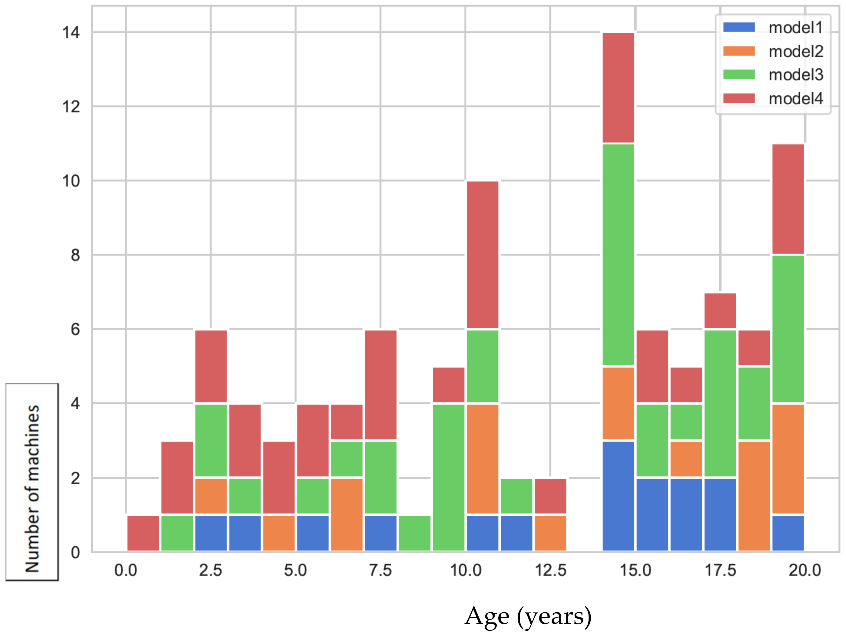
Figure 6.
Histogram representing the number of machines and service time, by model.

Figure 7.
Lag Features [9].
Figure 7.
Lag Features [9].

Figure 8.
Features correlation.

Figure 9.
Detailed analysis of the correlation between features pressuremean_3h and pressuremean_24h.
Figure 9.
Detailed analysis of the correlation between features pressuremean_3h and pressuremean_24h.

Figure 10.
Data classification and label construction—adapted from [9].
Figure 10.
Data classification and label construction—adapted from [9].


Table 1.
Typical example of real-time telemetry recording.
| Datetime | machineID | Volt | Rotate | Pressure | Vibration | |
|---|---|---|---|---|---|---|
| 0 | 2015-01-01 06:00:00 | 1 | 176.217853 | 418.504078 | 113.077935 | 45.087686 |
| 1 | 2015-01-01 07:00:00 | 1 | 162.879223 | 402.747490 | 95.460525 | 402.747490 |
| 2 | 2015-01-01 08:00:00 | 1 | 170.989902 | 527.349825 | 75.237905 | 34.178847 |
| 3 | 2015-01-01 09:00:00 | 1 | 162.462833 | 346.149335 | 109.248561 | 41.122144 |
| 4 | 2015-01-01 10:00:00 | 1 | 157.610021 | 435.376873 | 111.886648 | 25.990511 |
Table 2.
Statistical analysis of telemetry data in real time.
| Volt | Rotate | Pressure | Vibration | |
|---|---|---|---|---|
| count | 876100 | 876100 | 876100 | 876100 |
| mean | 170.777736 | 446.605119 | 100.858668 | 40.385007 |
| std | 15.509114 | 52.673886 | 11.048679 | 5.370361 |
| min | 97.333604 | 138.432075 | 51.237106 | 14.877054 |
| 25% | 160.304927 | 412.305714 | 93.498181 | 36.777299 |
| 50% | 170.607338 | 447.558150 | 100.425559 | 40.237247 |
| 75% | 181.004493 | 482.176600 | 107.555231 | 43.784938 |
| max | 255.124717 | 695.0209841 | 185.951998 | 76.791072 |
Table 3.
Typical error logging example.
| Datetime | machineID | errorID | |
|---|---|---|---|
| 0 | 2015-01-03 07:00:00 | 1 | error1 |
| 1 | 2015-01-03 20:00:00 | 1 | error3 |
| 2 | 2015-01-04 06:00:00 | 1 | error5 |
| 3 | 2015-01-10 15:00:00 | 1 | error4 |
| 4 | 2015-01-22 10:00:00 | 1 | error4 |
Table 4.
Typical example of maintenance records.
| Datetime | machineID | comp | |
|---|---|---|---|
| 0 | 2014-06-01 06:00:00 | 1 | comp2 |
| 1 | 2014-07-16 06:00:00 | 1 | comp4 |
| 2 | 2014-07-31 06:00:00 | 1 | comp3 |
| 3 | 2014-12-13 06:00:00 | 1 | comp1 |
| 4 | 2015-01-05 06:00:00 | 1 | comp 4 |
Table 5.
Typical example of failure records.
| Datetime | machineID | Failure | |
|---|---|---|---|
| 0 | 2015-01-05 06:00:00 | 1 | comp 4 |
| 1 | 2015-03-06 06:00:00 | 1 | comp 1 |
| 2 | 2015-04-20 06:00:00 | 1 | comp2 |
| 3 | 2015-06-19 06:00:00 | 1 | comp4 |
| 4 | 2015-09-02 06:00:00 | 1 | comp 4 |
Table 6.
Typical example of information for each machine.
| machineID | Model | Age | |
|---|---|---|---|
| 0 | 1 | model3 | 18 |
| 1 | 2 | model4 | 7 |
| 2 | 3 | model3 | 8 |
| 3 | 4 | model3 | 7 |
| 4 | 5 | model3 | 2 |
| 5 | 6 | model3 | 7 |
| 6 | 7 | model3 | 20 |
| 7 | 8 | model3 | 16 |
Table 7.
Example of Lag Features for telemetry data in real time, with N = 3.
| machineID | Datetime | Voltmean_3h | Rotatemean_3h | Pressuremean_3h | Vibrationmean_3h | |
|---|---|---|---|---|---|---|
| 0 | 1 | 2015-01-01 09:00:00 | 170.028993 | 449.533798 | 94.592122 | 40.893502 |
| 1 | 1 | 2015-01-01 12:00:00 | 164.192565 | 403.949857 | 105.687417 | 34.255891 |
| 2 | 1 | 2015-01-01 15:00:00 | 168.134445 | 435.781707 | 107.793709 | 41.239405 |
| 3 | 1 | 2015-01-01 18:00:00 | 165.514453 | 430.472823 | 101.703289 | 40.373739 |
| 4 | 1 | 2015-01-01 21:00:00 | 168.809347 | 437.111120 | 90.911060 | 41.738542 |
Table 8.
Example of Lag Features for telemetry data in real time, with N = 24.
| machineID | Datetime | Voltmean_24h | Rotatemean_24h | Pressuremean_24h | Vibrationmean_24h | |
|---|---|---|---|---|---|---|
| 7 | 1 | 2015-01-02 06:00:00 | 169.733809 | 445.179865 | 96.797113 | 40.385160 |
| 8 | 1 | 2015-01-02 09:00:00 | 170.614862 | 446.364859 | 96.849785 | 39.736826 |
| 9 | 1 | 2015-01-02 12:00:00 | 169.893965 | 447.009407 | 97.715600 | 39.498374 |
| 10 | 1 | 2015-01-02 15:00:00 | 171.243444 | 444.233563 | 96.666060 | 40.229370 |
| 11 | 1 | 2015-01-02 18:00:00 | 170.792486 | 448.440437 | 95.766838 | 40.055214 |
Table 9.
Example of Lag Features for error logging.
| machineID | Datetime | Error1count | Error2count | Error3count | Error4count | Error5count | |
|---|---|---|---|---|---|---|---|
| 15 | 1 | 2015-01-03 06:00:00 | 0.0 | 0.0 | 0.0 | 0.0 | 0.0 |
| 16 | 1 | 2015-01-03 09:00:00 | 0.0 | 0.0 | 0.0 | 0.0 | 0.0 |
| 17 | 1 | 2015-01-03 12:00:00 | 1.0 | 0.0 | 0.0 | 0.0 | 0.0 |
| 18 | 1 | 2015-01-03 15:00:00 | 1.0 | 0.0 | 0.0 | 0.0 | 0.0 |
| 19 | 1 | 2015-01-03 18:00:00 | 1.0 | 0.0 | 0.0 | 0.0 | 0.0 |
| 20 | 1 | 2015-01-03 21:00:00 | 1.0 | 0.0 | 0.0 | 0.0 | 0.0 |
| 21 | 1 | 2015-01-04 00:00:00 | 1.0 | 0.0 | 1.0 | 0.0 | 0.0 |
| 22 | 1 | 2015-01-04 03:00:00 | 1.0 | 0.0 | 1.0 | 0.0 | 0.0 |
| 23 | 1 | 2015-01-04 06:00:00 | 1.0 | 0.0 | 1.0 | 0.0 | 0.0 |
| 24 | 1 | 2015-01-04 09:00:00 | 1.0 | 0.0 | 1.0 | 0.0 | 1.0 |
Table 10.
Time since the last replacement, by type of component.
| Datetime | machineID | comp1 | comp2 | comp3 | comp4 | |
|---|---|---|---|---|---|---|
| 0 | 2015-01-01 06:00:00 | 1 | 19.000000 | 214.000000 | 154.000000 | 169.000000 |
| 1 | 2015-01-01 07:00:00 | 1 | 19.041667 | 214.041667 | 154.041667 | 169.041667 |
| 2 | 2015-01-01 08:00:00 | 1 | 19.083333 | 214.083333 | 154.083333 | 169.083333 |
| 3 | 2015-01-01 09:00:00 | 1 | 19.125000 | 214.125000 | 154.125000 | 169.125000 |
| 4 | 2015-01-01 10:00:00 | 1 | 19.166667 | 214.166667 | 154.166667 | 169.166667 |
Table 11.
Example of failure representation in component 2.
| machineID | Datetime | Model | Age | Failure | |
|---|---|---|---|---|---|
| 857 | 1 | 2015-04-19 09:00:00 | model3 | 18 | comp2 |
| 858 | 1 | 2015-04-19 12:00:00 | model3 | 18 | comp2 |
| 859 | 1 | 2015-04-19 15:00:00 | model3 | 18 | comp2 |
| 860 | 1 | 2015-04-19 18:00:00 | model3 | 18 | comp2 |
| 861 | 1 | 2015-04-19 21:00:00 | model3 | 18 | comp2 |
| 862 | 1 | 2015-04-20 00:00:00 | model3 | 18 | comp2 |
| 863 | 1 | 2015-04-20 03:00:00 | model3 | 18 | comp2 |
| 864 | 1 | 2015-04-20 06:00:00 | model3 | 18 | comp2 |
| 2297 | 1 | 2015-10-16 09:00:00 | model3 | 18 | comp2 |
| 2298 | 1 | 2015-10-16 12:00:00 | model3 | 18 | comp2 |
| 2299 | 1 | 2015-10-16 15:00:00 | model3 | 18 | comp2 |
| 2300 | 1 | 2015-10-16 18:00:00 | model3 | 18 | comp2 |
| 2301 | 1 | 2015-10-16 21:00:00 | model3 | 18 | comp2 |
| 2302 | 1 | 2015-10-17 00:00:00 | model3 | 18 | comp2 |
| 2303 | 1 | 2015-10-17 03:00:00 | model3 | 18 | comp2 |
| 2304 | 1 | 2015-10-17 06:00:00 | model3 | 18 | comp2 |
Table 12.
Amount of data attributed to each of the sets and the percentage corresponding to failures.
Table 12.
Amount of data attributed to each of the sets and the percentage corresponding to failures.
| Quantity | /% | Failure/% |
|---|---|---|
| Training | 66.52 | 2.02 |
| Validation | 16.57 | 1.89 |
| Test | 16.91 | 1.92 |
Table 13.
Example of the imbalance between the different classes for the ‘failure’ feature in the total data set.
Table 13.
Example of the imbalance between the different classes for the ‘failure’ feature in the total data set.
| Failure | % | |
|---|---|---|
| none | 285,684 | 98.06 |
| comp2 | 1985 | 0.68 |
| comp1 | 1464 | 0.50 |
| comp4 | 1240 | 0.43 |
| comp3 | 968 | 0.33 |
Table 14.
Performance for the Random Forest model in the validation and test sets, with ’n_estimators = 70.
Table 14.
Performance for the Random Forest model in the validation and test sets, with ’n_estimators = 70.
| None | comp1 | comp2 | comp3 | comp4 | |
|---|---|---|---|---|---|
| Precision | 0.9997 | 0.9244 | 0.9916 | 1.0000 | 0.9812 |
| Conj. Develop. Recall | 0.9999 | 0.9578 | 0.9861 | 0.9514 | 0.9543 |
| F1 Score | 0.9998 | 0.9408 | 0.9889 | 0.9751 | 0.9676 |
| Precision | 0.9988 | 0.9718 | 0.9711 | 0.9855 | 0.9830 |
| Conj. Test Recall | 0.9998 | 0.8150 | 0.9882 | 0.9189 | 0.9611 |
| F1 Score | 0.9993 | 0.8865 | 0.9796 | 0.9510 | 0.9719 |
Table 15.
Performance for the Artificial Neural Network model in the validation and test sets, with 100 hidden layers (hidden layers = 100) and min-max scaling normalization.
Table 15.
Performance for the Artificial Neural Network model in the validation and test sets, with 100 hidden layers (hidden layers = 100) and min-max scaling normalization.
| None | comp1 | comp2 | comp3 | comp4 | |
|---|---|---|---|---|---|
| Precision | 0.9997 | 0.9451 | 0.9917 | 1.0000 | 0.9520 |
| Conj. Develop.Recall | 0.9998 | 0.9337 | 0.9972 | 0.9167 | 0.9954 |
| F1 Score | 0.9997 | 0.9394 | 0.9945 | 0.9565 | 0.9732 |
| Precision | 0.9990 | 0.9030 | 0.9941 | 0.9858 | 0.9725 |
| Conj. Test Recall | 0.9995 | 0.8425 | 0.9853 | 0.9392 | 0.9833 |
| F1 Score | 0.9993 | 0.8717 | 0.9897 | 0.9619 | 0.9779 |
Publisher’s Note: MDPI stays neutral with regard to jurisdictional claims in published maps and institutional affiliations. |
© 2020 by the authors. Licensee MDPI, Basel, Switzerland. This article is an open access article distributed under the terms and conditions of the Creative Commons Attribution (CC BY) license (http://creativecommons.org/licenses/by/4.0/).
Share and Cite
MDPI and ACS Style
Cardoso, D.; Ferreira, L. Application of Predictive Maintenance Concepts Using Artificial Intelligence Tools. Appl. Sci. 2021, 11, 18. https://doi.org/10.3390/app11010018
AMA Style
Cardoso D, Ferreira L. Application of Predictive Maintenance Concepts Using Artificial Intelligence Tools. Applied Sciences. 2021; 11(1):18. https://doi.org/10.3390/app11010018
Chicago/Turabian StyleCardoso, Diogo, and Luís Ferreira. 2021. "Application of Predictive Maintenance Concepts Using Artificial Intelligence Tools" Applied Sciences 11, no. 1: 18. https://doi.org/10.3390/app11010018
Note that from the first issue of 2016, this journal uses article numbers instead of page numbers. See further details here.