Convex Model for Estimation of Single-Phase Photovoltaic Impact on Existing Voltage Unbalance in Distribution Networks


Department of Electrical Engineering and Automation, Aalto University, Maarintie 8, 02150 Espoo, Finland
*
Author to whom correspondence should be addressed.
Appl. Sci. 2020, 10(24), 8884; https://doi.org/10.3390/app10248884
Submission received: 31 October 2020
/
Revised: 9 December 2020
/
Accepted: 9 December 2020
/
Published: 12 December 2020
(This article belongs to the Special Issue Power Quality in Electrical Power Systems)
Abstract
:Due to the increasing adoption of solar power generation, voltage unbalance estimation gets more attention in sparsely populated rural networks. This paper presents a Monte Carlo simulation augmented with convex mixed-integer quadratic programming to estimate voltage unbalance and maximum photovoltaic penetration. Additionally, voltage unbalance attenuation by proper phase allocation of photovoltaic plants is analysed. Single-phase plants are simulated in low-voltage distribution networks and voltage unbalance is evaluated as a contribution of measured background and photovoltaic-caused unbalance. Voltage unbalance is calculated in accordance with EN 50160 and takes into account 10-minute average values with 5% tolerance condition. Results of the optimization revealed substantial unbalance attenuation with optimal phase selection and increased potential of local generation hosting capacity in case of higher background unbalance.
1. Introduction
The widespread increase in distributed energy generation has raised much attention in planning and operation of distribution networks. A myriad of networks were built decades ago and they were designed in accordance with unidirectional power flow. Nowadays, network operators are looking into finding operational limits of existing networks, concurrently learning to design networks that would be suited for distributed generation in the future. Such a demand has sparked new wave of estimation and optimization of network operation. On par with voltage level violations, voltage unbalance (VU) is one of the main issues that causes concerns for network operators. As local power generation becomes more accessible to wider masses of customers, more single-phase devices are connected to networks, causing VU. As the latest review indicates [1], the VU limits nearly fifth of the cases of photovoltaic (PV) integration. The unbalance problem becomes more severe in sparsely populated areas, and becomes a major limiting factor of solar energy integration in rural distributed networks.
Voltage unbalance is defined by few institutions, however the commonly accepted true definition of VU is defined in standard EN 50160. The VU is a ratio of negative and positive sequence components of three-phase voltage phasors. In case of any asymmetry in voltage phasors, the negative sequence component increases, starting from zero. In perfectly balanced networks, the positive sequence component equals to phase voltage and remains relatively unchanged even during unbalance condition. The limit is set to 2% during 95% of a week in 10-min time resolution. The true formulation of VU was compared with three other VU definitions in Ref. [2]. The analysis revealed that VU calculation results can drastically vary depending on the formulation, thus having a common reference point is important while conducting VU studies.
Numerous works have been done on assessing VU levels in networks with PVs or any other kind of distributed generation. In [3], authors proposed simple, yet effective methodology for VU assessment. The proposed method does not require load flow calculations and just estimates VU based on negative sequence current contribution of each PV. Different single-phase PV connection strategies were shown and extensive sensitivity analysis was showcased on several sized networks. The model, however, did not represent simulations over a week-long period. A probabilistic modelling of distribution network was demonstrated in [4]. Time series of PV generation and load were analysed and utilized in quasi-sequential Monte Carlo simulation for the further assessment of voltage-level and unbalanced violations. The importance of the cumulative duration of violations was emphasized in the article, since network standards set the violation tolerance on one week basis. Another probabilistic analysis of VU based on the Monte Carlo simulation is presented in [5]. The contribution of several VU sources was utilized to prospect possible VU mitigation possibilities. The impact of network line configuration on VU and power factor of PVs was demonstrated.
A VU sensitivity analysis was performed in [6] for different PV sizes and location in case of typical networks in Spain. Probabilistic PV and load models were utilized to assess VU in rural networks. It showcased lower VU levels at urban networks, while rural networks sustain severe VU. To properly evaluate network standard requirements, a recommended PV size was derived based on one-year simulations on 10-minute mean resolution. Randomness of PV installations, such as number of PVs, PV location and others, was modelled with Monte Carlo simulation.
An evaluation of VU mitigation by PVs is analyzed in [7]. Mitigation schemes were modelled with probabilistic approach in a Monte Carlo simulation. The study is focused on long-term operation of networks concerning VU mitigation schemes. Calculations are supported by a three-phase load flow algorithm and utilize historical metered data. A comprehensive analysis of PV impact on distribution network and its hosting capacity (HC) was carried out in [8]. The study covered 50,000 real low-voltage distribution networks and considered several limiting constraints, including VU. The hosting capacity was presented in risk-based analysis, where the network HC is represented as a probability value. Thus, it is possible to derive a risk level that a network operator is willing to take. Moreover, traditional Monte Carlo simulations were carried out in [9,10] to assess VU and its extent to PV hosting capacity.
Several works focused on the contribution of many VU sources at customer buses. An extensive analysis was carried out in [11], which divided VU contributors into downstream and upstream (background) sources. The Thevenin approach was utilized to allocate contributors into two parts and then each part was individually split down into sub-units. An aggregation of VU components was studied in [12]. A wide range of VU factors was modelled and their contribution at every distribution network bus was evaluated.
Voltage unbalance estimation by Monte Carlo simulation can predict possible VU levels and is useful in determining solar HC of distribution networks. As observed in the articles previously, most of the Monte Carlo simulations have fixed PV output and the exact value of HC remains unresolved. On the other hand, an optimization routine with PV output as a decision variable changes the direction of the VU estimation and permits new possibilities for HC studies. Exact HC value, that would satisfy VU constraint, can be found. According to the true definition, VU is a division of two complex numbers. Such a division in decision variable leads to a nonlinear and nonconvex constraint, which steer researchers towards heuristic solving approaches.
In recent years, numerous articles presented heuristics with optimal power flow, where VU was one out of several constraints. A study on VU optimization with heuristic algorithm was presented in [13]. The nonlinear nature of the problem formulation is tackled by the particle swarm optimization. Electric vehicle dispatch strategies and their efficiency on VU mitigation were presented. A hybrid method of stochastic optimization, genetic algorithm and fuzzy logic was proposed in [14]. Losses and VU of a three-phase distribution network were minimized with respect to voltage and ampacity limits. A dynamic scenario generation was proposed to tackle the probabilistic nature of PV generation. The presented VU calculation is based on the true definition of VU based on sequence components, and thus the model is nonconvex.
The genetic algorithm was utilized in [15] to tackle the nonconvexity of the load flow and VU formulation. While minimizing VU, load flow algorithm was executed with the holomorphic embedding method. As a part of multiobjective electric network optimization, VU minimization was presented in [16]. A novel differential evolution algorithm was employed for the optimization and VU was calculated based on nonconvex sequence components, that were provided by nonlinear load flow algorithm. An empirical continuous metaheuristic was compared with several other heuristic algorithms in [17]. VU minimization was a part of multiobjective function, and, as in previously mentioned works, VU formulation retained nonconvexity.
Heuristic algorithms are resilient to tackle nonlinear problems easily. They provide good balance between optimality and runtime. However, they do not guarantee a global solution. Increased computational efficiency of modern computers have allowed researchers to deploy alternative optimization algorithms based on mathematical programming. Contrary to heuristics, mathematical optimization grants global solution for a convex problem. Therefore, the convex formulation of a problem becomes more crucial for mathematical optimization.
Network optimization by mathematical programming was conducted in several works. A three-phase network optimization for optimal energy storage dispatch algorithm was presented in [18]. To convexify the model, the VU formulation was relaxed by substituting voltage positive sequence component by the nominal voltage value. In such a way, the division of two decision variables was excluded. Another convex model was presented in [19]. The model was adopted in VU compensation mechanism in microgrids, and formulated the VU constraint as a quadratically constrained programming. However, the model lacks integer variables for the phase selection of single-phase prosumers. A comprehensive robust optimization of day-ahead operation planning was presented in [20]. The problem is formulated as a mixed-integer nonlinear model, which is then linearized and applied in two-stage optimization. The VU is formulated with sequence components, however the positive sequence component is substituted in a similar manner as in [18]. The negative sequence component is calculated on a branch current basis, and the real and imaginary parts of the current are split into two separate variables, before they are merged in a quadratic constraint.
The semidefinite programming was utilized to optimize the operation of three-phase network in [21]. The method was then applied for soft open point device, that balanced network voltages by reactive power injection. The original nonlinear, nonconvex problem was reformulated into convex semidefinite programming task. The VU was advocated as the maximum deviation of the average voltage levels, thus abandoning the commonly considered true VU definition. As mentioned previously, holding on to the true definition is vital for VU studies. However, in order to convexify the true VU definition, a minor relaxation of the definition is required. Most of the articles employed nominal voltage value as a substitute for positive sequence voltage. It is a decent relaxation due to safer overestimation of the VU, and is a justified sacrifice to reach convex formulation. However, in real life, the positive sequence voltage fluctuates and leaves varying margin for VU. Instead, the utilization of measured positive sequence voltage would provide slightly more accurate relaxation of the VU definition.
In the light of aforementioned concerns, this paper presents a convex VU optimization method that is paired with the Monte Carlo simulation. The model is based on bus injection transfer impedance model, and as in [3], does not require load flow calculations, making the presented approach fast and suitable for repetitive calculations. The convexity of presented VU definition is achieved by substituting positive sequence voltage by corresponding measured weekly data. Furthermore, VU calculation incorporates 5% violation tolerance during a week on 10-minute resolution. Moreover, the effect of background VU fluctuation on the HC is analyzed with respect to fixed and variable phase selection of single-phase PV plants. The hosting capacity of this article is found solely with respect to VU.
The rest of the paper is structured as follows. Data utilized and its modification is explained in Section 2. Monte Carlo simulation is described in Section 3. Initial formulation of the problem and its convex reformulation are presented in Section 4 and Section 5. Results of the simulations are shown in Section 6, followed by conclusions in Section 7.
2. Measured Data
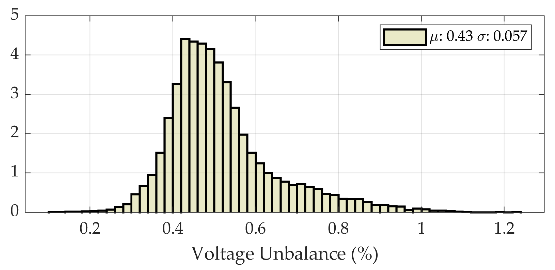
Measured weekly data are utilized as a reference level of VU. Measurement campaign was carried out in 2018 in Helsinki region, Finland, where voltages of secondary substations were recorded. An in-depth presentation of measured data can be found in [22]. Data employed in the current paper comprise phase and line voltages at 10-minute time resolution. Eight weeks of measured data are available for sampling in the Monte Carlo simulation. The three phasors of voltages are processed by symmetrical component transformation into positive and negative sequence components. Both of the components are used to calculate background voltage unbalance, that is depicted in a summarized Figure 1.
2.1. Prevailing Ratio
Prevailing ratio (PR) is utilized to quantify the level of variation of background negative sequence voltage over a week. Higher variability is a result of frequent change of phasor angle and magnitude, that is reflected in lower PR value. Since VU is evaluated as a 95th percentile value of 1008 time steps of a week, higher variability will result in higher VU in the Monte Carlo simulation due to the cumulative effect. Prevailing ratio for single week can be calculated as shown in Equation (1) [23].
of Equation (1) is background negative sequence phasor at a time instance t, that is in the set of 1008 instances of a week . Prevailing ratio is a numerical value between zero and one. Weeks with PR close to one can be characterized as high prevalence. Individual negative sequence phasors have high similarity and they do not alter over a week. Such a background VU can be easily attenuated by a static vector, that is opposing to the vector of the background VU. On the other hand, PR value of 0.95 and lower is considered as medium and low prevalence. An attenuating negative sequence vector would need to follow the changes of background unbalance. However, if angular and magnitude changes of attenuating vector are not possible, then average VU will tend to increase.
2.2. Added Variability
A random deviation of voltage magnitude and angle was added to the model to add variety to PR values. Firstly, average value and standard deviation in each phase of measured voltage are found, as mentioned in Equation (2). The difference value is then found for each time instance t by subtracting phase voltage from corresponding average value (Equation (3)). Thirdly, an offset value is sampled from a uniform distribution, that ranges from zero to double of the standard deviation, as shown in Equation (4). Finally, the offset is added to the voltage value in case of negative deviation from the mean value. Otherwise the offset is subtracted, as shown in Equation (5). The sets are defined in Equation (6). After the angles of measured phasors follow the same procedure as described above, the sequence components are derived.
3. Monte Carlo Simulation
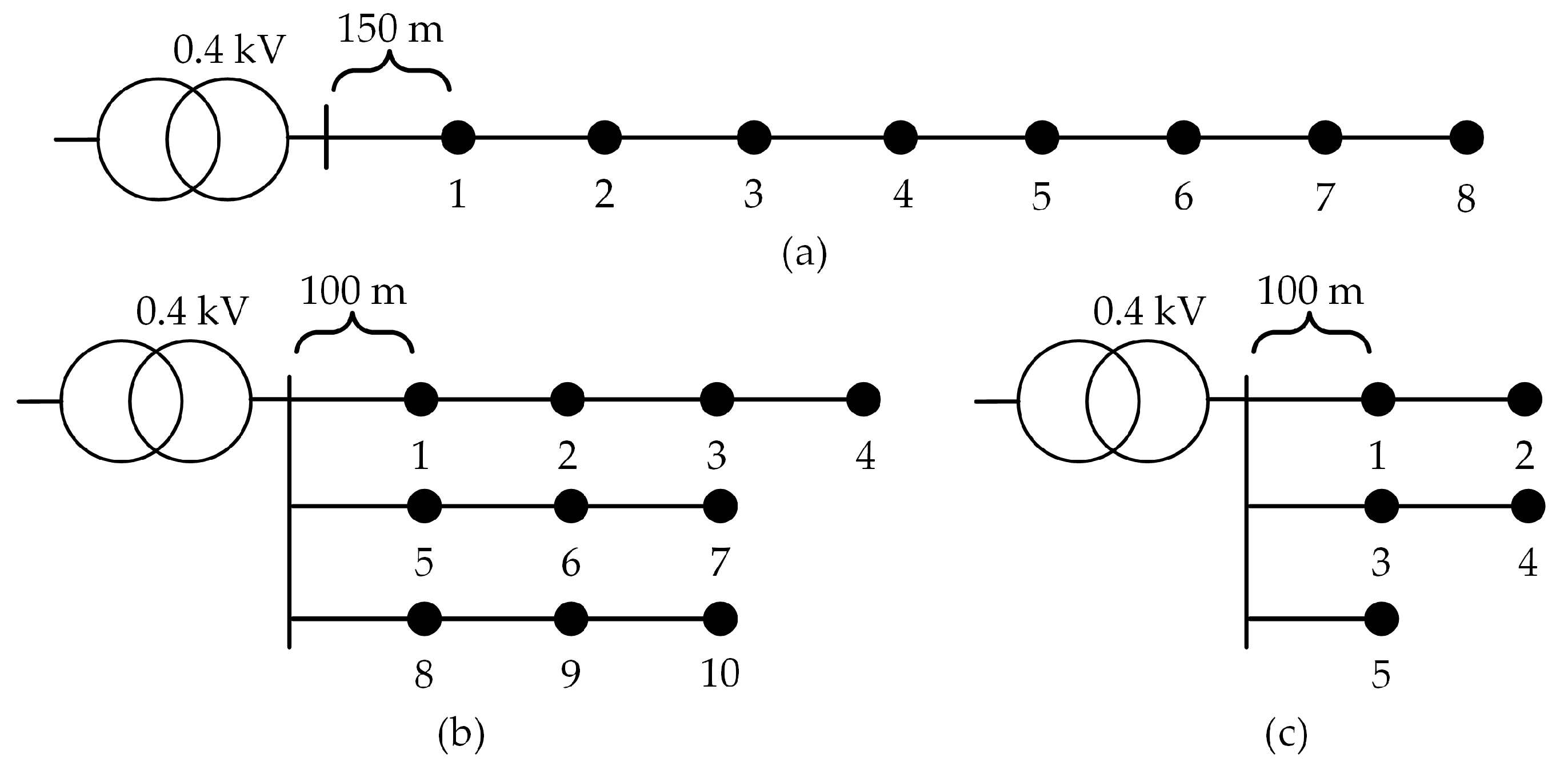
Presented framework is tested on three types of networks that are typical for distribution systems in Finland. The networks represent rural, suburban and urban areas and possess different topology, number of customers and line parameters. The networks are depicted in Figure 2. A summary of the regions modelled is shown in Table 1, and an extensive description of the networks and their formation is explained in [24]. The power of the single PV plant is assumed to be equal to a single phase circuit of 16 A, which corresponds to kWp at nominal voltage. Such power will be further referred to as the single-phase circuit capacity. PV plants are assumed to be constant power models and their contribution to negative sequence current is of the total injected current at nominal voltage.
3.1. Number of Photovoltaics
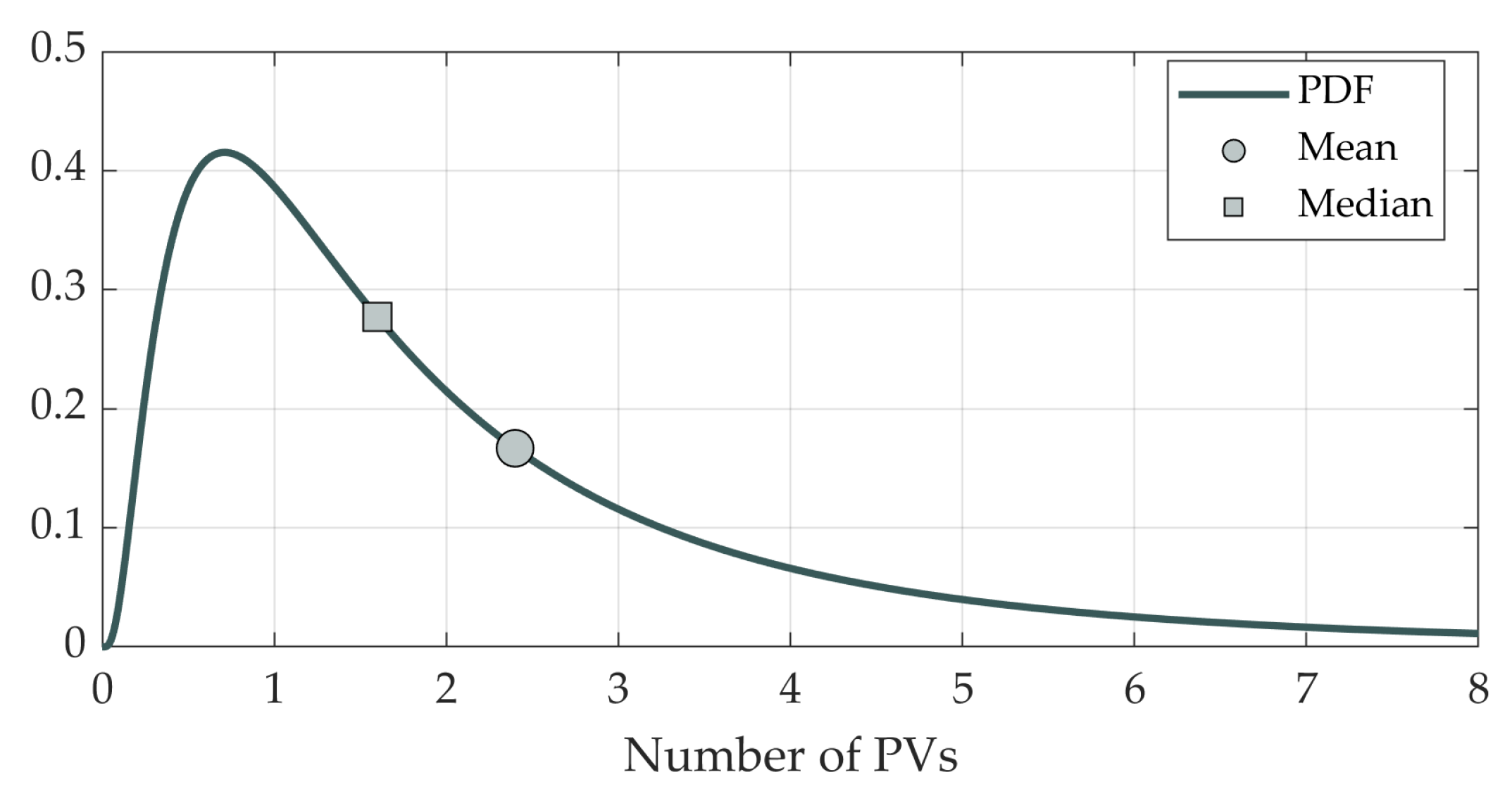
To sample the number of PVs in a network, a lognormal distribution is employed. In [25], the statistical summary of PV plants is presented, which reveals average and median sizes of PV plants in Finland. To formulate the sampling of number of PVs, two assumptions are made. Firstly, the number of PVs follows a lognormal distribution. Secondly, due to the fixed power of a PV plant in the presented work, the lognormal distribution is utilized for sampling number of PVs, instead of sampling size of a PV plant. The PV plant size values in aforementioned article are equal to kWp and kWp. The acquired ratio of for mean and median values for lognormal distribution is kept and utilized to calculate standard deviation, as shown in Equation (7).
The average and median peak power of PV plants are interpreted as the number of PVs. The average number is assumed to be equal to 30% of the total number of customers in a network, e.g., in case of the rural network, the average number of PVs equals . This assumption is based on the research in [25], which concludes that PVs are profitable for one third of the residential building stock in Helsinki metropolitan area. Due to the wide range of population density in the area, such estimation is utilized in suburban and urban networks as well. Once the distribution parameters are found, the lognormal distribution is then formulated as . The probability distribution functions of the rural network are depicted in Figure 3.
3.2. Connection Strategies
In order to analyze the impact of PV on VU levels and HC of networks, four phase connection strategies are simulated. The strategies will determine the phases that single-phase PVs will be connected to. The strategies are listed below.
- Strategy 1—Random phasePV plants are connected to a randomly sampled phase among the phases a, b and c with equal probability.
- Strategy 2—Sequential phase, starting with phase aPV plants are connected in a sequential order a-b-c-a-…
- Strategy 3—Sequential phase, starting from random phaseThe starting phase of the phase sequence is sampled randomly. The sequence then follows same pattern as in strategy 2.
- Strategy 4—The phase with lowest voltageThe phase with lowest voltage is estimated by the negative sequence voltage phasor. The angle of the negative sequence voltage phasor is compared to the angles of the phases, and the phase with highest angular difference is chosen as the connection phase.
3.3. Structure of the Simulation
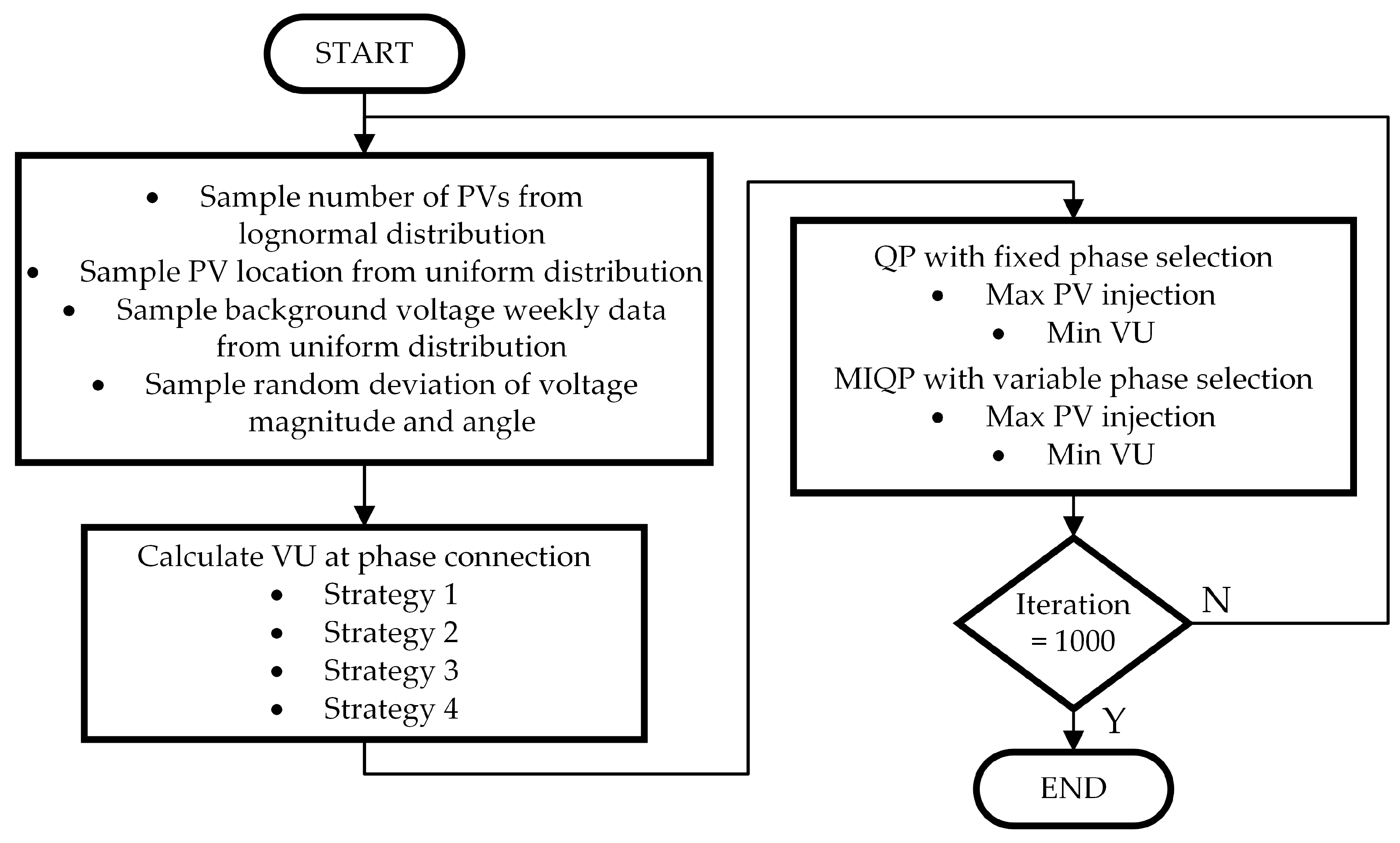
The Monte Carlo simulation comprises 1000 iterations, after the results are saved. As shown in Monte Carlo simulations of [3,6,10], 1000 iterations are enough to maintain stable results. The simulation starts with sampling random input variables. Number of PVs in the network is sampled from the lognormal distribution, that is presented below. The location of PVs is sampled with uniform distribution. Every PV plant has a bus associated with it and only one PV plant can occupy a bus. One-week measured voltage data is sampled from the 8 weeks of measured data. Every measured week has the same probability to be chosen for current iteration. Finally, deviations of magnitude and angle of each phase voltage are randomly sampled to provide higher variety of background VU, as described in Section 2.2. In the next step, VU is calculated for all the strategies. Input parameters, that were sampled in previous step, are kept the same for all the strategies. Voltage unbalance is calculated for each 10-minute time step of one week. Then, a 95th percentile value of each bus is calculated. The highest VU value is then saved for result analysis. During the third step of the Monte Carlo simulation, the optimization routine is initiated. Since the PV injection value fluctuates along a week, the most conservative minimum value is chosen at first to represent PV injection. However, to take into account the tolerance condition allowed by the standard, 5th percentile value of PV injection is found at each bus and then saved for further analysis. The flowchart of the simulation can be seen in Figure 4.
4. Transfer Impedance
The transfer impedance is utilized to calculate the contribution of each PV to the negative sequence voltage. Transfer impedance is a i by j matrix, that transfers PV contribution column of length i into voltage drop column of length j. The magnitude of the injected current is the value of the negative sequence current and the angle of the negative sequence current depends on the phase that is chosen. It is assumed that connected PVs are synchronized with background voltage phasors and their injected current follows the angle of background voltage phasors.
The main concept of the transfer impedance utilization in this paper is inspired by [3]. However, minor changes were introduced to the transfer impedance matrix. In order to include several customers with PVs per one bus, additional columns were included in the matrix. Customers, that are connected to one bus, have the same contribution to the VU. Additionally, customer nodes, that have no PV, thus no contribution to the negative sequence voltage, are pruned from the transfer impedance matrix, as well as from the current injection column. The negative sequence voltage, as a sum of background and PV-caused negative sequence voltage, can be found as followed in Equation (8).
where is total negative sequence voltage, is transfer impedance, is PV-injected negative sequence current, is background negative sequence component obtained from phase voltages in Equation (5), is a set of network buses and is a set of buses with PVs. Note that the variables presented are phasors, and constitute magnitude and angle values.
5. Convex Reformulation
The model shown in Equation (8) is reformulated into an optimization problem. A quadratic programming (QP) formulation is presented first, that considers phase selection as a parameter passed by the strategies listed in Section 3.2. Later, phase selection is changed into decision variable, and together with PV injection current decision variable, forms a mixed-integer quadratic programming (MIQP) problem. Both of the formulations are presented in two objective functions: maximize PV injection and minimize VU. Maximizing PV can be portrayed as finding HC. Even though HC calculations generally consider more constraints than just VU, the presented model can be interpreted as PV hosting capacity with respect to VU.
5.1. Fixed Phase
The PV injection maximization problem with fixed phase selection is formulated below. The objective function encapsulates the total sum of PV injection at all buses with PV, at any phase and any time, denoted in Equation (9).
The PV-injected current is split into real and imaginary parts, as shown in (10). The real phase angle values are given by measured phasor data and are fixed parameters during optimization routine. Thus, the cosine and sine functions are both constants, that are scaling the injected current value by the phase and angle of voltage phasors. In (11), the real and imaginary parts of the negative sequence voltage are calculated, reflecting the contribution of a single PV plant. The background-measured voltage component is added to the PV contribution. The condition of equal PV contribution is set in Equation (12). It is assumed that all PVs are in close vicinity and they are exposed to the same amount of irradiance. The real and imaginary parts of the negative sequence voltage are merged back in the quadratic Equation (13). Convexity condition is granted by the linearity of voltage components. Real and imaginary parts of the negative sequence voltage are found as a linear function of the decision variable (PV-injected power). The sum of squared linear functions is convex, hence the problem is convex and the global solution can be found. The negative sequence voltage magnitude is limited to 2% of background positive sequence voltage in (14). To keep the convexity, measured data are utilized in the VU denominator. Such relaxation is fair, as the true positive sequence voltage tends to increase during PV network feed. The utilized values are smaller, thus staying on the safe side and underestimating available headroom for PV injection. The big-M concept is applied in (15) to limit injected current to zero in case of phases that have no PV plants. The is an arbitrary large positive value and is equal to 100 in current calculations. The sets are defined in (16) and are valid for all the equations presented above. All presented variables are non-negative.
The VU minimization problem is based on the model presented above. All the constraints are the same, except for the objective function. As shown in Equation (17), the objective function is the sum of negative sequence voltages at every bus and all time instances.
5.2. Variable Phase
The phase parameter is now changed to a free binary variable, which converts the problem into MIQP. The binary variable adds to the complexity of the problem. The objective function, however, remains as compared to the previous case, and is maximizing the total PV current injection, as in Equation (18).
While the majority of the equations remain, the phase selection variable causes changes in the set of constraints. As previously, the big-M concept is utilized in (19) to restrain current from reaching positive values in phases that are free from PV plants. Condition in (20) holds if a PV plant at node i is connected only to one phase . Two- and three-phase PVs are thus not feasible. The set of time interval is changed to two time instances in (21). All newly introduced variables are non-negative. Due to the high computational complexity of mixed-integer task, the time interval set consists of the time instance with the highest and the lowest background VU, as compared to the fixed phase case, where the time interval covers full week on 1008 10-minute values. The VU minimization problem holds little changes compared to previous formulations, and consists of previously prepared equations. The problem is composed as follows.
6. Results
In this section, results of VU assessment with Monte Carlo simulation and optimization paired with Monte Carlo simulations are presented. Moreover, an analysis of PR and PV distance on the HC is presented. Due to the low VU levels in suburban and urban networks, the optimization is showcased only at the rural network. Monte Carlo simulation was programmed in MATLAB R2020a, while both the QP and MIQP formulations of the problem were programmed in GAMS. GAMS was accessed via a MATLAB interface and results were analyzed in MATLAB. The CPLEX solver was chosen for both of the porblem formulations. A workstation equipped with an Intel Xeon 3.40 GHz processor and 16 GB of RAM was used to run the simulations.
6.1. Monte Carlo Simulation
The results of the Monte Carlo simulation are presented below. The rural network presented in Figure 5 reveals high levels of VU, exceeding 2% limit. The only strategy that is able to keep VU below the limit, is strategy 4. Another great benefit of strategy 4 is the low variance of the results. The VU levels are less likely to deviate from an average value. Strategies 2 and 3 result in quite similar VU levels with relatively low variance. Figure 6 shows results of suburban (a) and urban (b) networks. VU levels never exceed VU limit over the course of this simulation. The higher impact of single-phase PVs can be noticed in suburban networks, since the difference of variance of strategies 1 and 4 is high. Compared to the urban network, the variance does not change within strategies. This indicates a dominant role of background VU source on the total VU.
6.2. Optimization Fixed Phase
In the previous section, over the course of current simulations, VU levels always stay below the 2% limit in case of suburban and urban networks. Consequently, further optimization is focused on the rural network.
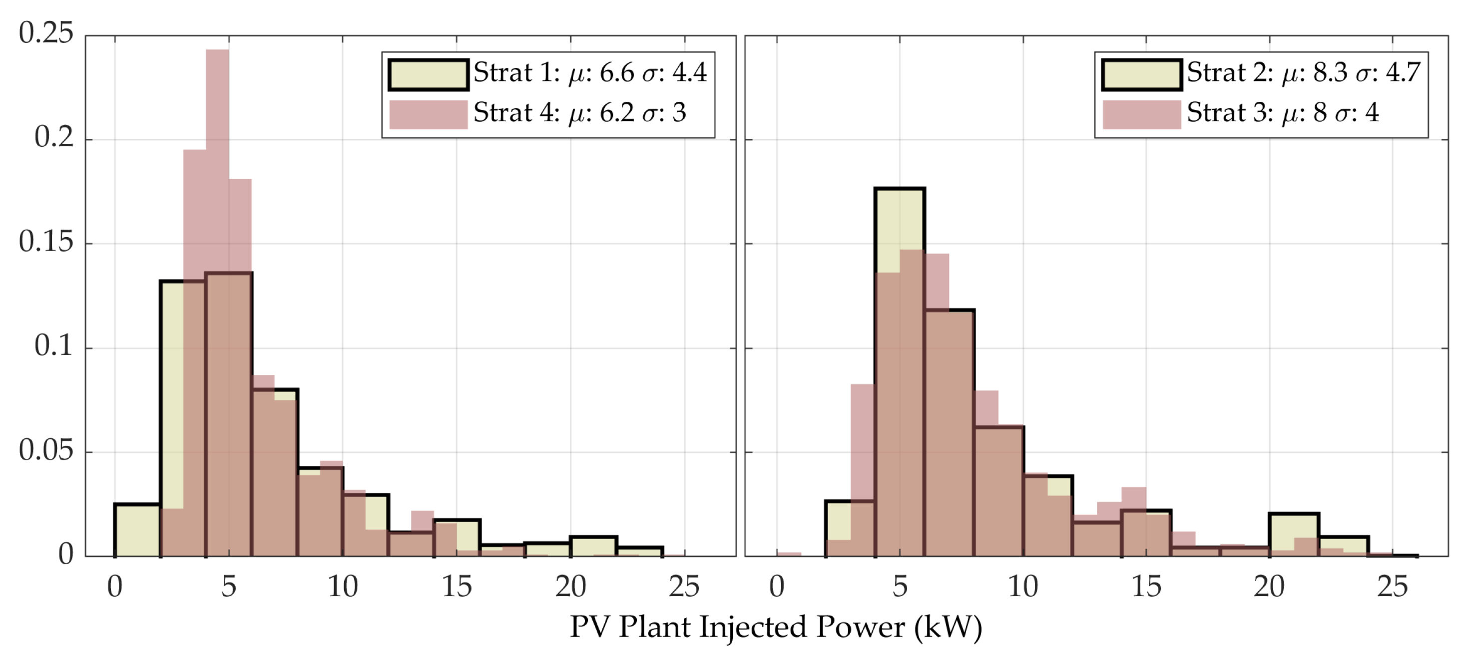
The results of the QP problem formulation are presented. PV phase connection was fixed as entailed by the strategies. The histogram of maximum PV injected current can be seen in Figure 7. As concluded by visual inspection, the histograms follow lognormal distribution. As expected, strategy 1 performs worse than strategy 2 and 3. Phase selection that on average causes high VU will result in lower average HC. Strategies 2 and 3 are once again quite similar, except to the bump around 20–25 kW for strategy 2. Starting the phase sequence at phase a at all the times will guarantee to show good result in part of randomly generated scenarios. Strategy 4, however, demonstrates the worst performance. The reason behind bad results is the changes of the negative sequence voltage vector. The phases of strategy 4 are fixed in the case where PV injected power is equal to the single-phase circuit capacity at particular background VU. However, if the injected power of PV plants is increased, the relative contribution of background unbalance to the resultant unbalance vector is decreasing. By increasing injected power even further, PV plants must rearrange connection phases to mitigate increasing unbalance caused by themselves. Phase selection must be reconsidered every time after the power is altered. The adaptive phase selection is better demonstrated in optimization with variable phases in Section 6.3.
Recapping the VU histogram in Figure 5, a validation of the two figures can be made. In VU assessment, the PV injection was fixed and VU values were recorded. On the contrary, the VU limit is fixed in the maximization, and the PV injection is a variable. Both of the estimations are essentially focused around one point. To justify the percentile values of 95 of VU and 5 of PV power, the comparison is shown in Table 2.
The number of instances VU exceeding 2% limit is shown in the first row, remembering that the PV plant power in Monte Carlo simulation is equal to single-phase circuit capacity. Likewise, the number of cases PV plant power of Figure 7 is below the single-phase circuit capacity shown in the bottom row of the table. The values have a close match, except for strategy 4. As discussed above, connection phases of strategy 4 are selected, while the PV injected power is fixed to single-phase circuit capacity. During the optimization, however, the power is altered and the phase selection must be reconsidered for every unique power value. The optimal selection of the phases is presented in forthcoming section. Other strategies, however, suggest the validity of the 5th percentile PV power estimation as an equivalent reference value for tolerance condition set by tthe EN 50160 standard. The small difference though can be explained by the equal power condition for PV plants, while the VU obtains a unique value for every bus.
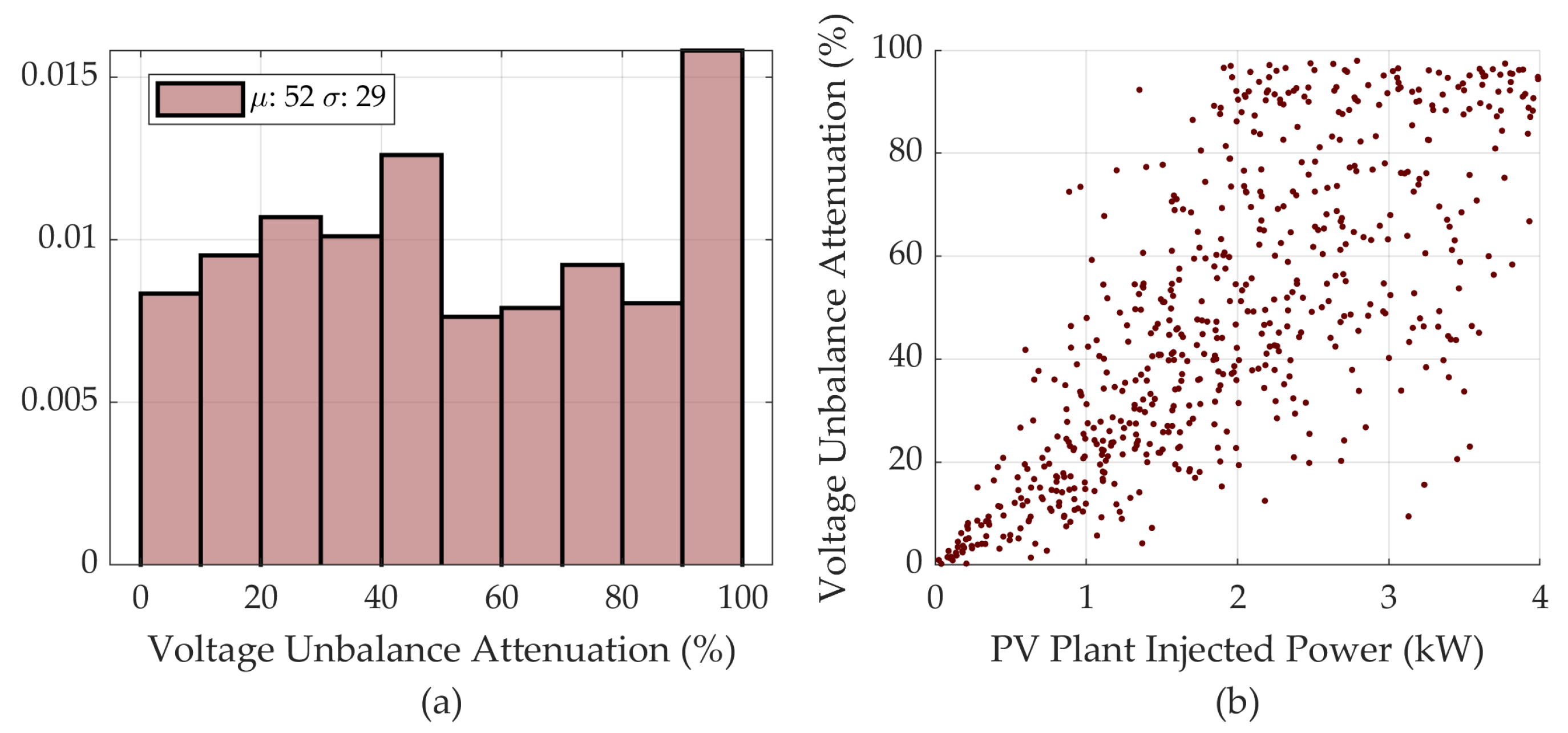
The results of minimizing the VU at fixed phase connection are shown in Figure 8. The histogram of VU attenuation is shown on (a), where it can be seen, that attenuation is hindered by the phase selection of the strategy 3 and strongly depends on the background VU phasor. Due to the fact that the phasor angle is fixed to the feeding voltage phasor, the attenuating vectors of single-phase PVs are not able to follow the vector of the background VU, and the attenuation is not always possible, as indicates the average attenuation value of 52%. As compared to other results of current paper, voltage unbalance mitigation subject to fixed phases is the only case where some iterations yield no improving result. Voltage unbalance was attenuated in 69.1% of the cases generated in Monte Carlo simulation. The VU attenuation with respect to PV injected current is shown in (b). Vague linear relationship can be noticed between the attenuation and injected power. Within successful iterations, the single-phase circuit capacity was able to minimize VU in 85.6% of the tries. Full attenuation of VU can be achieved at relatively low power values.
6.3. Optimization Variable Phase
Next, the problem formulations are altered by changing the phase selection parameter into a decision variable. A binary decision variable is the reason of MIQP problem classification and significantly increases computation complexity. The results below are presented for two cases: the lowest and highest background VU over a week.
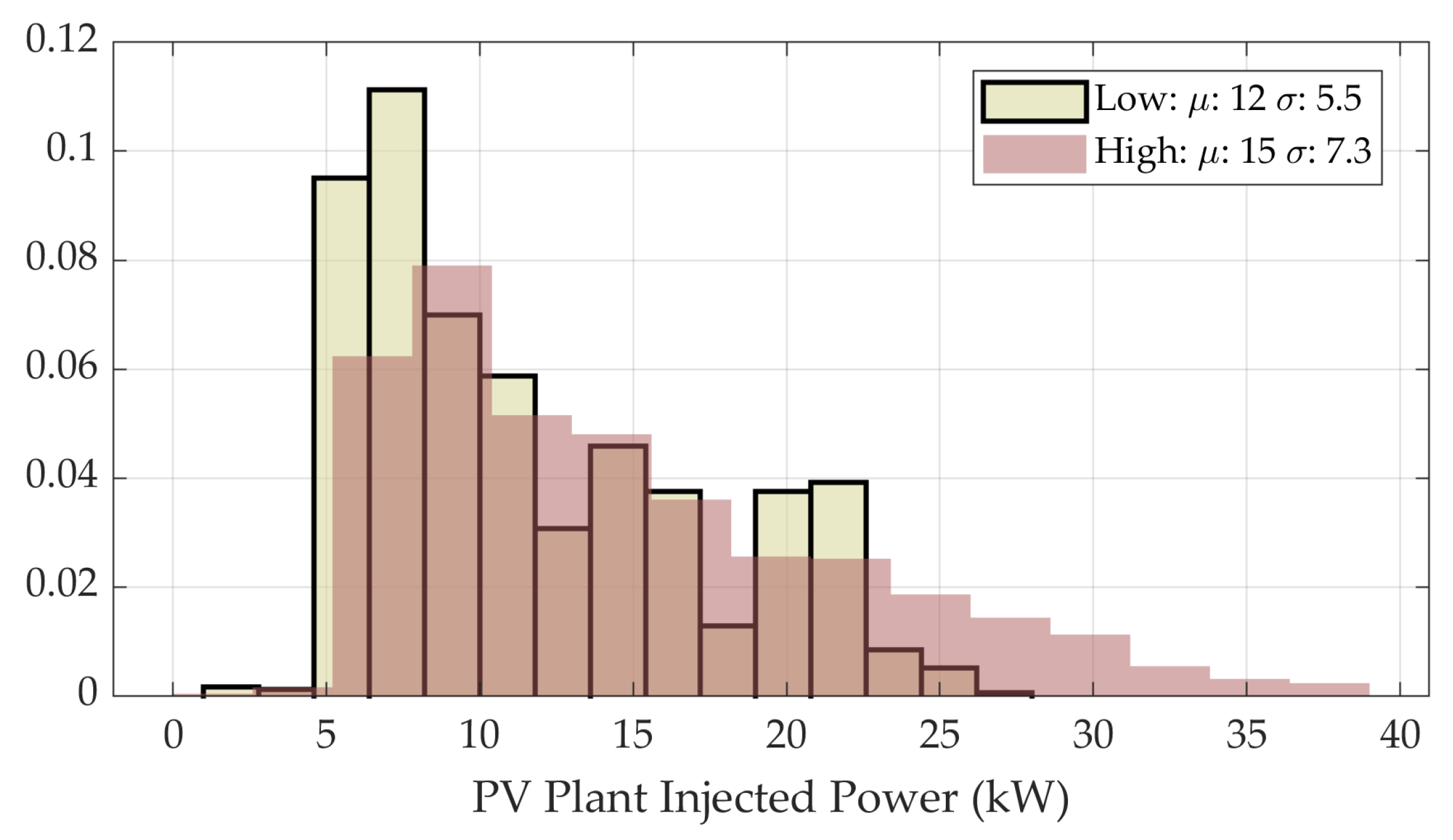
The histogram of maximum injected power is presented in Figure 9. Finding the optimal phase selection results in high PV injection. The average value of injected current nearly double of that of strategies 2 and 3 in Figure 7. In comparison with high VU, the average value of injected current at low VU is lower, the reason being that more PV power is directed to VU mitigation. The peak injection reaches values as large as 35 kW.
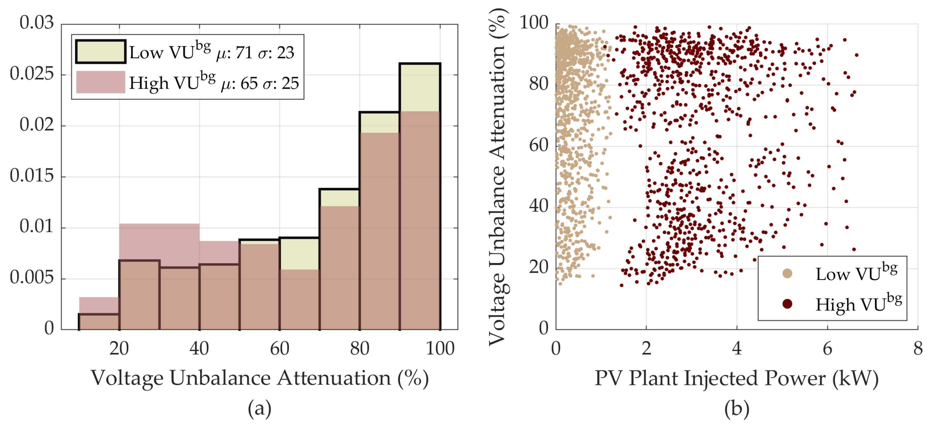
VU attenuation at variable phase is shown in Figure 10, where (a) reveals, that despite the higher injected power shown on the figure above, the average VU attenuation is lower at high background VU. In contrast to the fixed phase, the VU is attenuated to higher extent at variable phase selection. Additionally, optimal phase selection results in VU attenuation at all the times, as none of the instances on subplot (b) are within close vicinity of 0% attenuation, as compared to Figure 8b. Moreover, the attenuation is achieved at minor power injections. Furthermore, 99.9% of time instances with the lowest background unbalance were attenuated by the power lower than the single-phase circuit capacity. In case of the highest background unbalance, attenuation by the single-phase circuit was in 71.7% of the iterations.
6.4. Max PV with Respect to PR
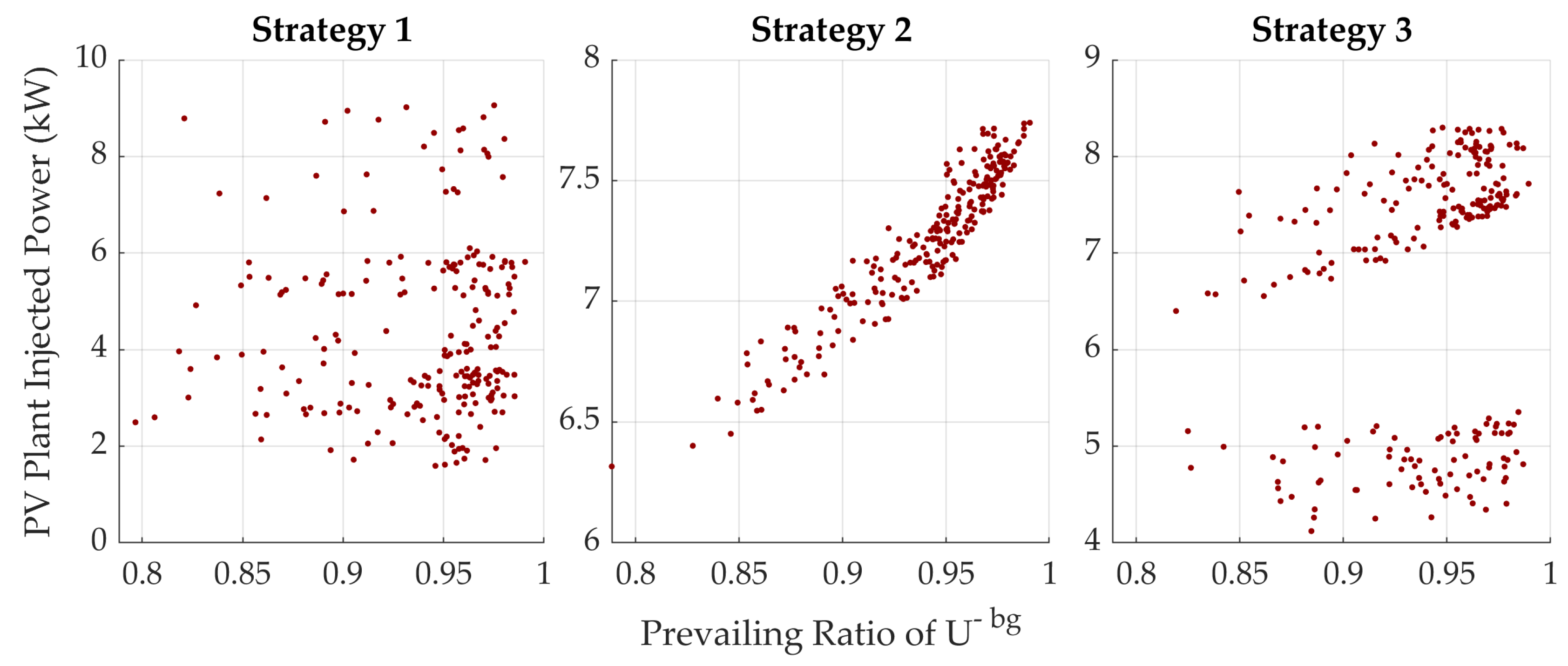
The results of the PR sensitivity analysis are presented in Figure 11. In order to reveal the effect of PR, some values within Monte Carlo simulation were fixed. The number of PVs was fixed to 3, the location of PVs was fixed to buses 2, 5 and 8. Finally, one measured data array was used, that was modified as previously described in Section 2.
In case of phase connection strategy 1, the PR of background negative sequence voltage has almost no effect of HC. Maximum PV injection is governed by other parameters, such as phase selection. Chaotic phase connection causes high VU and the background unbalance has smaller relative contribution. However, if the phases are fixed, as in the case of strategy 2, a trend starts to be revealed. The maximum injection falls as the PR value deviates from 1. Strategy 3 underlines the above-mentioned conclusions. Three clusters of results can be distinguished in case of strategy 3, that corresponds to the starting phase of sequential phase selection. Low PR has negative impact on maximum PV injection at favourable starting phase. On the other hand, PR has no impact on the least favourable starting phase, as the PV-caused VU is dominating the total unbalance.
6.5. Max PV with Respect to Average Distance
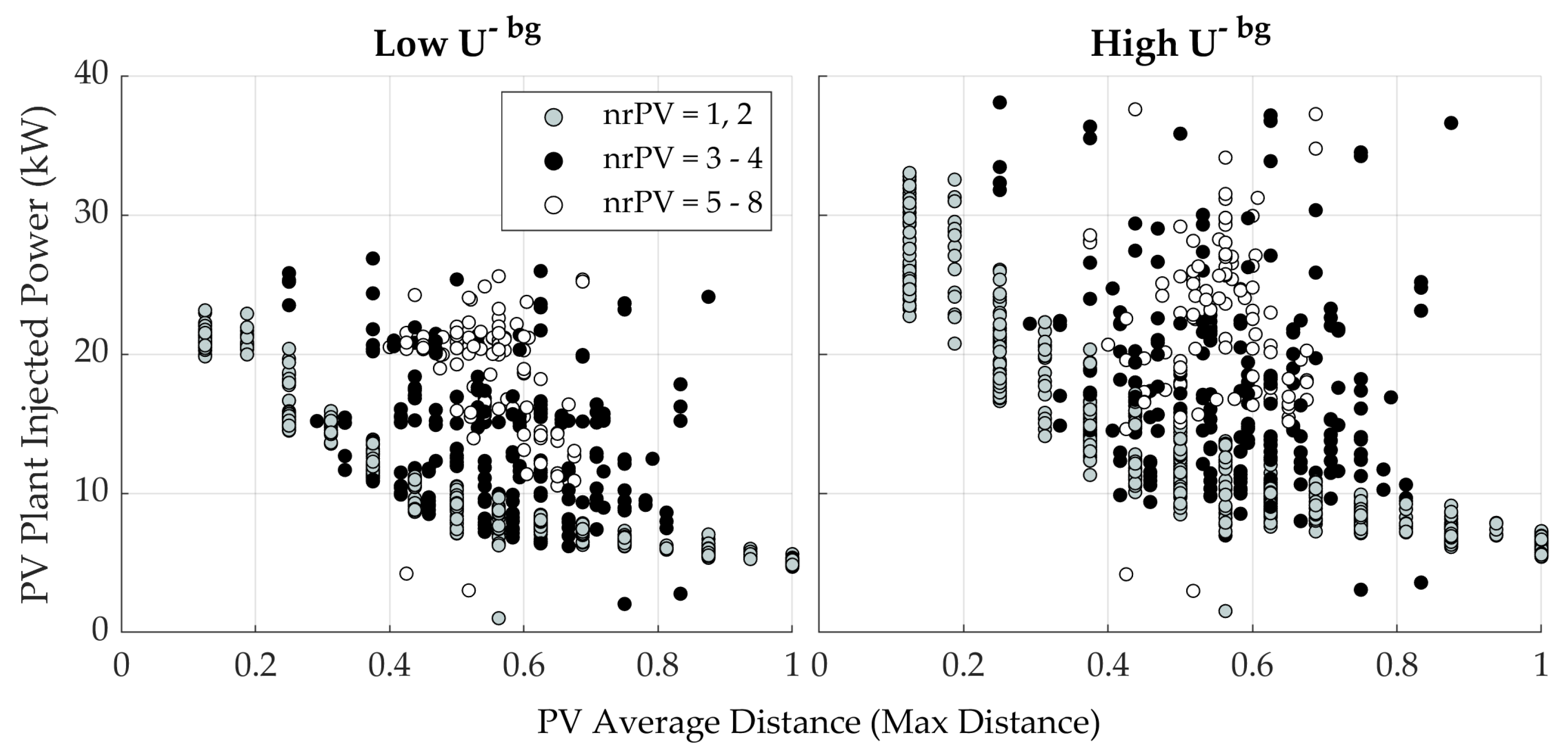
Maximum injected PV current is analyzed with respect to average distance of PVs in Figure 12. Two cases of variable phase selection are presented: low and high background VU. Despite the slight difference in PV injected power, a similar trend can be seen in both cases. At a small number of PVs (one or two PV plants), the maximum injection is correlated with average distance, whereas at a higher number of PVs (three and four PV plants), the trend is less prominent. As even more PVs are added to the network, their average distance converges to 0.5, measured as relative distance to the farthest-most bus. If the network is almost completely full of PVs, unbalance is cancelled out by fellow PVs, and VU is less of a concern, as it is reflected in high PV injection results.
6.6. Computation Time
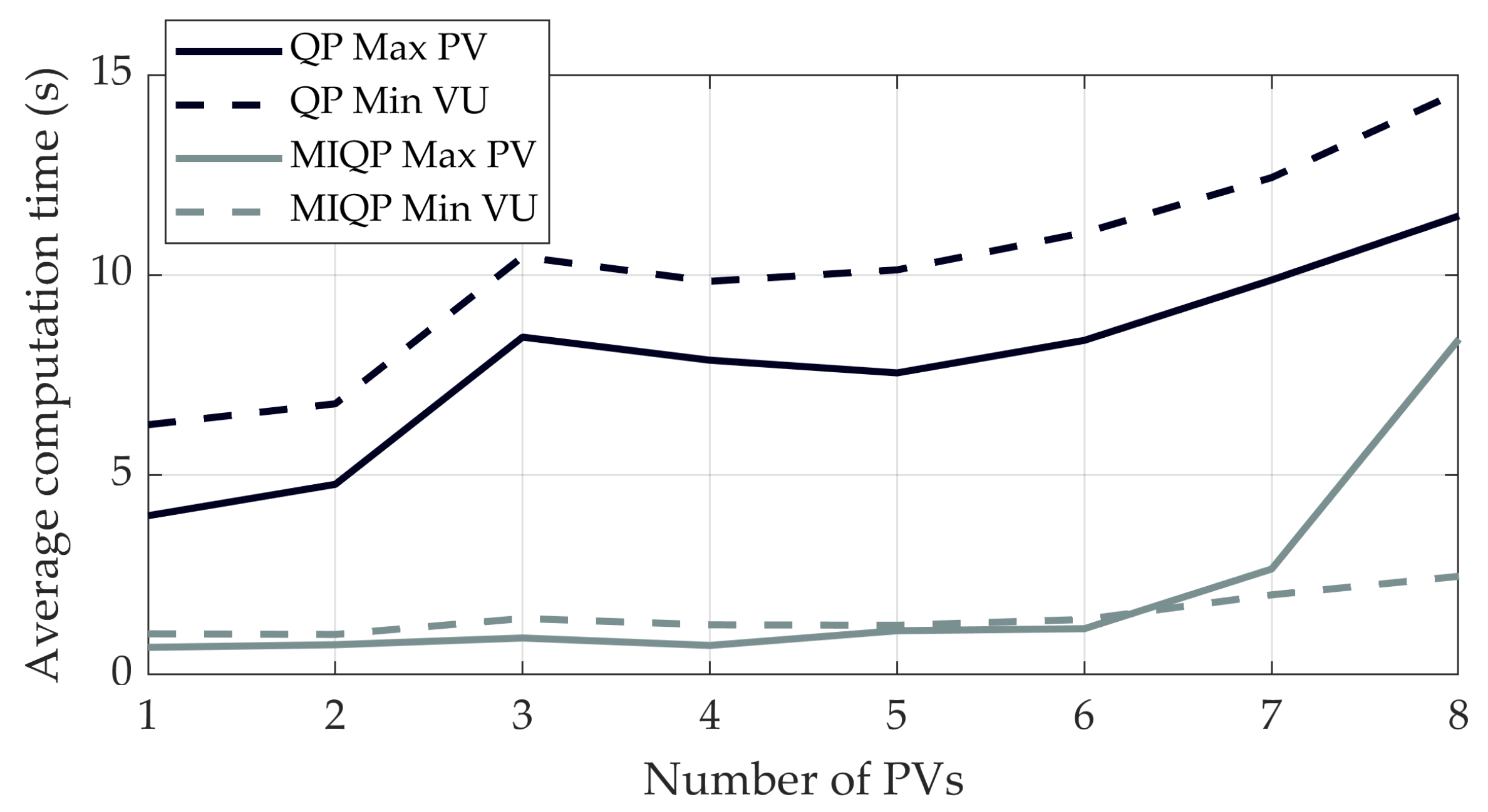
Finally, computation times of the optimization algorithms are presented in Figure 13. Moreover, 50 Monte Carlo simulations were conducted for each number of PVs in the rural network. Computation times were then averaged over 50 iterations and plotted as a function of PV number. In order to provide fair ground for comparison, added variability functions were disabled, such as variability of background voltage unbalance. Additionally, only one week of measured data was employed in comparison, and due to the fixed start of the sequential connection, strategy 2 was chosen for QP problems.
The QP problem formulation implies optimization with fixed phases. The PV injected current is defined over three sets, where i denotes number of PVs and denotes number of phases. Due to the fixed phase selection, the set of phases entails only one variable. Lastly, index t covers 1008 time steps of 10-minute values over one week. The MIQP problem formulation implies variable phase selection of single-phase PVs in the model, which adds binary variables into the formulation. On the other hand, the number of time steps under consideration is reduced to two. Hence, the complexity of the decision variable is defined over number of PVs i, three binary variables and the lowest and the highest background voltage unbalance time instances t. The relative gap of the mixed-integer problem is equal to zero in all the simulation instances.
7. Conclusions
This paper presented a convex VU optimization method that is paired with Monte Carlo simulation. The model showcases the benefit of convex model with relaxed VU definition, that was used for stochastic assessment of distribution network HC. The bus-injection model of the problem formulation enabled to estimate VU without load-flow calculations. Measured weekly voltage data were utilized for background VU modelling and total VU was estimated on 5% weekly tolerance condition. Similarly to [20], the convex relaxation of VU definition shows a credible result.
As in [6], the results indicated higher VU levels at rural networks. Problem formulation with fixed phase selection showed maximum allowable PV injection to be limited by the background VU. Problem formulation with variable phase, however, demonstrated the ability of single-phase PVs to nearly double PV power injection. Higher background VU grants higher HC. As seen in other papers, consideration of other constraints, such as voltage limits, start to be more important. Optimal phase selection of single-phase PVs eliminates issue and other limits start to be the bottleneck for HC [18]. Furthermore, both fixed and variable phase models showed ability to attenuate VU considerably. PVs with power of the single-phase circuit capacity can attenuate VU in range of 70–99% of the simulated cases.
Analysis of background negative sequence voltage variability, that is quantified by PR, revealed lower HC in case of predictable phase selection strategies, e.g., sequential phase selection. On the other hand, random phase selection of PVs will lead to almost no correlation between HC and PR. Moreover, the paper summarizes that PV HC is higher, if PVs are located closer to feeding substation. Lastly, the computation times of the presented algorithms are within the same range as the similarly formulated problem in [18].
Author Contributions
Conceptualization, V.P. and M.L.; methodology, V.P.; software, V.P.; validation, V.P. and M.L.; formal analysis, V.P.; investigation, V.P.; resources, M.L.; data curation, M.L.; writing—original draft preparation, V.P.; writing—review and editing, V.P.; visualization, V.P.; supervision, M.L.; project administration, M.L.; funding acquisition, M.L. All authors have read and agreed to the published version of the manuscript.
Funding
This research was funded by Business Finland as a part of “SolarX” project.
Acknowledgments
The authors of the paper would like to extend their gratitude towards Helen Sähköverkko Oy and Caruna Networks Oy for benevolent help in conducting measurements.
Conflicts of Interest
The authors declare no conflict of interest.
Abbreviations
The following abbreviations and nomenclature are used in this manuscript:
| HC | Hosting capacity |
| MIQP | Mixed-integer quadratic programming |
| PR | Prevailing ratio |
| PV | Photovoltaic |
| QP | Quadratic programming |
| VU | Voltage unbalance |
| Sets | |
| Set of network buses | |
| Set of buses with PVs | |
| Set of two time steps with the lowest and highest background VU | |
| Set of 1008 steps of a week on 10-minute time resolution | |
| Set of phases a, b and c | |
| Indices | |
| i, j, k | Indices of buses |
| t | Index of time step |
| Index of phases | |
| Variables | |
| Variable phase selection binary matrix | |
| Negative sequence current injected by PV | |
| , | Real and imaginary parts of the injected PV current |
| Negative sequence voltage | |
| and | Real and imaginary parts of the negative sequence voltage |
| Parameters | |
| Fixed phase selection binary matrix | |
| Big-M parameter | |
| , | Resistance and reactance of the transfer impedance matrix |
| Background positive sequence voltage | |
| and | Real and imaginary parts of the background negative sequence voltage |
| Phase angle |
References
- Samar, F.; Püvi, V.; Lehtonen, M. Review on the PV Hosting Capacity in Distribution Networks. Energies 2020, 13, 4756. [Google Scholar] [CrossRef]
- Girigoudar, K.; Roald, L.A. On the impact of different voltage unbalance metrics in distribution system optimization. Electr. Power Syst. Res. 2020, 189, 106656. [Google Scholar] [CrossRef]
- Schwanz, D.; Möller, F.; Ronnberg, S.K.; Meyer, J.; Bollen, M.H.J. Stochastic Assessment of Voltage Unbalance Due to Single-Phase-Connected Solar Power. IEEE Trans. Power Deliv. 2017, 32, 852–861. [Google Scholar] [CrossRef]
- Silva, E.N.; Rodrigues, A.B.; da Guia da Silva, M. Stochastic assessment of the impact of photovoltaic distributed generation on the power quality indices of distribution networks. Electr. Power Syst. Res. 2016, 135, 59–67. [Google Scholar] [CrossRef]
- Liu, Z.; Milanovic, J.V. Probabilistic Estimation of Voltage Unbalance in MV Distribution Networks With Unbalanced Load. IEEE Trans. Power Deliv. 2015, 30, 693–703. [Google Scholar] [CrossRef]
- Ruiz-Rodriguez, F.; Hernández, J.; Jurado, F. Voltage unbalance assessment in secondary radial distribution networks with single-phase photovoltaic systems. Int. J. Electr. Power Energy Syst. 2015, 64, 646–654. [Google Scholar] [CrossRef]
- Klonari, V.; Meersman, B.; Bozalakov, D.; Vandoorn, T.L.; Vandevelde, L.; Lobry, J.; Vallée, F. A probabilistic framework for evaluating voltage unbalance mitigation by photovoltaic inverters. Sustain. Energy Grids Netw. 2016, 8, 1–11. [Google Scholar] [CrossRef]
- Torquato, R.; Salles, D.; Oriente Pereira, C.; Meira, P.C.M.; Freitas, W. A Comprehensive Assessment of PV Hosting Capacity on Low-Voltage Distribution Systems. IEEE Trans. Power Deliv. 2018, 33, 1002–1012. [Google Scholar] [CrossRef]
- Dubey, A.; Santoso, S.; Maitra, A. Understanding photovoltaic hosting capacity of distribution circuits. In Proceedings of the 2015 IEEE Power & Energy Society General Meeting, Denver, CO, USA, 26–30 July 2015; pp. 1–5. [Google Scholar] [CrossRef]
- Kharrazi, A.; Sreeram, V.; Mishra, Y. Assessment of voltage unbalance due to single phase rooftop photovoltaic panels in residential low voltage distribution network: A study on a real LV network in Western Australia. In Proceedings of the 2017 Australasian Universities Power Engineering Conference (AUPEC), Melbourne, Australia, 19–22 November 2017; pp. 1–6. [Google Scholar] [CrossRef] [Green Version]
- Sun, Y.; Li, P.; Li, S.; Zhang, L. Contribution Determination for Multiple Unbalanced Sources at the Point of Common Coupling. Energies 2017, 10, 171. [Google Scholar] [CrossRef] [Green Version]
- Abasi, M.; Ghodratollah Seifossadat, S.; Razaz, M.; Sajad Moosapour, S. Determining the contribution of different effective factors to individual voltage unbalance emission in n-bus radial power systems. Int. J. Electr. Power Energy Syst. 2018, 94, 393–404. [Google Scholar] [CrossRef]
- Farahani, H.F. Improving voltage unbalance of low-voltage distribution networks using plug-in electric vehicles. J. Clean. Prod. 2017, 148, 336–346. [Google Scholar] [CrossRef]
- Xu, J.; Wang, J.; Liao, S.; Sun, Y.; Ke, D.; Li, X.; Liu, J.; Jiang, Y.; Wei, C.; Tang, B. Stochastic multi-objective optimization of photovoltaics integrated three-phase distribution network based on dynamic scenarios. Appl. Energy 2018, 231, 985–996. [Google Scholar] [CrossRef]
- Rao, B.; Kupzog, F.; Kozek, M. Three-Phase Unbalanced Optimal Power Flow Using Holomorphic Embedding Load Flow Method. Sustainability 2019, 11, 1774. [Google Scholar] [CrossRef] [Green Version]
- Islam, M.R.; Lu, H.; Hossain, J.; Islam, M.R.; Li, L. Multiobjective Optimization Technique for Mitigating Unbalance and Improving Voltage Considering Higher Penetration of Electric Vehicles and Distributed Generation. IEEE Syst. J. 2020, 14, 3676–3686. [Google Scholar] [CrossRef]
- Coelho, F.; Peres, W.; Silva Junior, I.; Dias, B. An Empirical Continuous Metaheuristic for Multiple Distributed Generation Scheduling Considering Energy Loss Minimization, Voltage and Unbalance Regulatory Limit. IET Gener. Transm. Distrib. 2020, 14, 3301–3309. [Google Scholar] [CrossRef]
- Watson, J.D.; Watson, N.R.; Lestas, I. Optimized Dispatch of Energy Storage Systems in Unbalanced Distribution Networks. IEEE Trans. Sustain. Energy 2018, 9, 639–650. [Google Scholar] [CrossRef]
- De Oliveira Luna, J.D.F.; Jose, D.; Renato da Costa Mendes, P.; Normey-Rico, J.E. A Convex Optimal Voltage Unbalance Compensator for Hybrid AC/DC Microgrids. In Proceedings of the 2019 IEEE PES Innovative Smart Grid Technologies Conference—Latin America (ISGT Latin America), Gramado, Brazil, 15–18 September 2019; pp. 1–6. [Google Scholar] [CrossRef]
- Sepehry, M.; Kapourchali, M.H.; Aravinthan, V.; Jewell, W. Robust Day-Ahead Operation Planning of Unbalanced Microgrids. IEEE Trans. Ind. Inform. 2019, 15, 4545–4557. [Google Scholar] [CrossRef]
- Li, P.; Ji, H.; Wang, C.; Zhao, J.; Song, G.; Ding, F.; Wu, J. Optimal Operation of Soft Open Points in Active Distribution Networks Under Three-Phase Unbalanced Conditions. IEEE Trans. Smart Grid 2019, 10, 380–391. [Google Scholar] [CrossRef]
- Püvi, V.; Tukia, T.; Lehtonen, M.; Kütt, L. Survey of a Power Quality Measurement Campaign in Low-Voltage Grids. In Proceedings of the 2019 Electric Power Quality and Supply Reliability Conference (PQ) & 2019 Symposium on Electrical Engineering and Mechatronics (SEEM), Kärdla, Estonia, 12–15 June 2019; pp. 1–7. [Google Scholar] [CrossRef] [Green Version]
- Möller, F.; Meyer, J. Survey on emission characteristic of the symmetrical components of voltage and current in LV grids. In Proceedings of the 2018 18th International Conference on Harmonics and Quality of Power (ICHQP), Ljubljana, Slovenia, 13–16 May 2018; pp. 1–6. [Google Scholar] [CrossRef]
- Arshad, A.; Lindner, M.; Lehtonen, M. An Analysis of Photo-Voltaic Hosting Capacity in Finnish Low Voltage Distribution Networks. Energies 2017, 10, 1702. [Google Scholar] [CrossRef] [Green Version]
- Vimpari, J.; Junnila, S. Estimating the diffusion of rooftop PVs: A real estate economics perspective. Energy 2019, 172, 1087–1097. [Google Scholar] [CrossRef]
Figure 1.
Background voltage unbalance.

Figure 2.
Networks modeled for rural (a), suburban (b) and urban (c) regions.

Figure 3.
Lognormal distribution used for sampling the number of PVs in rural network.

Figure 4.
Flowchart of the Monte Carlo simulation.

Figure 5.
Voltage unbalance levels in rural network.

Figure 6.
Voltage unbalance in suburban (a) and urban (b) networks.

Figure 7.
Maximum PV injection at fixed phases.

Figure 8.
Voltage unbalance attenuation at strategy 3 (a) and corresponding PV injection (b).

Figure 9.
Maximum PV injection at optimal phase selection.

Figure 10.
Voltage unbalance attenuation with optimal phase (a) and corresponding PV injection (b) at the lowest and highest background VU.
Figure 10.
Voltage unbalance attenuation with optimal phase (a) and corresponding PV injection (b) at the lowest and highest background VU.

Figure 11.
Maximum PV injection at different PR values of background VU.

Figure 12.
Maximum PV injection at different PV average distance from the substation.

Figure 13.
Average computation time.


Table 1.
Test network parameters.
| Region | Transformer Rating (kVA) | Cable Length (m) | Cable Type | No. of Feeders | Buses per Feeder | Customers Per Bus | Average No. of PVs |
|---|---|---|---|---|---|---|---|
| Rural | 50 | 150 | 70 mm2 | 1 | 8 | 1 | 2.4 |
| Suburban | 200 | 100 | 185 mm2 | 3 | 4, 3, 3 | 4 | 12 |
| Urban | 1000 | 100 | 2 × 185 mm2 | 3 | 2, 2, 1 | 60 | 90 |
Publisher’s Note: MDPI stays neutral with regard to jurisdictional claims in published maps and institutional affiliations. |
© 2020 by the authors. Licensee MDPI, Basel, Switzerland. This article is an open access article distributed under the terms and conditions of the Creative Commons Attribution (CC BY) license (http://creativecommons.org/licenses/by/4.0/).
Share and Cite
MDPI and ACS Style
Püvi, V.; Lehtonen, M. Convex Model for Estimation of Single-Phase Photovoltaic Impact on Existing Voltage Unbalance in Distribution Networks. Appl. Sci. 2020, 10, 8884. https://doi.org/10.3390/app10248884
AMA Style
Püvi V, Lehtonen M. Convex Model for Estimation of Single-Phase Photovoltaic Impact on Existing Voltage Unbalance in Distribution Networks. Applied Sciences. 2020; 10(24):8884. https://doi.org/10.3390/app10248884
Chicago/Turabian StylePüvi, Verner, and Matti Lehtonen. 2020. "Convex Model for Estimation of Single-Phase Photovoltaic Impact on Existing Voltage Unbalance in Distribution Networks" Applied Sciences 10, no. 24: 8884. https://doi.org/10.3390/app10248884
Note that from the first issue of 2016, this journal uses article numbers instead of page numbers. See further details here.