Article

Reconstruction of Late Pleistocene-Holocene Deformation through Massive Data Collection at Krafla Rift (NE Iceland) Owing to Drone-Based Structure-from-Motion Photogrammetry

1
Department of Earth and Environmental Sciences, University of Milan-Bicocca, I-20126 Milan, Italy
2
CRUST-Interuniversity Center for 3D Seismotectonics with Territorial Applications, I-66100 Chieti Scalo, Italy
*
Author to whom correspondence should be addressed.
Appl. Sci. 2020, 10(19), 6759; https://doi.org/10.3390/app10196759
Submission received: 25 August 2020 / Revised: 21 September 2020 / Accepted: 24 September 2020 / Published: 27 September 2020

Abstract

:
In the present work, we demonstrate how drone surveys coupled with structure-from-motion (SfM) photogrammetry can help to collect huge amounts of very detailed data even in rough terrains where logistics can affect classical field surveys. The area of study is located in the NW part of the Krafla Fissure Swarm (NE Iceland), a volcanotectonic rift composed of eruptive centres, extension fractures, and normal faults. The surveyed sector is characterized by the presence of a hyaloclastite ridge composed of deposits dated, on a stratigraphic basis, to the Weichselian High Glacial (29.1–12.1 ka BP), and a series of lava flows mostly dating back to 11–12 ka BP. The integration of remotely sensed surveys and field inspections enabled us to recognize that this segment of the Krafla rift is made of grabens arranged en-échelon with a left-stepping geometry. A major graben increases in width in correspondence of the hyaloclastite cone; we interpret this geometry as resulting from the mechanical contrast between the stiffer lava succession and the softer hyaloclastites, which favours the development of concentric faults. We also measured a total extension of 16.6 m and 11.2 m along the fractures affecting the lava units, and a total extension in the hyaloclastites of 29.3 m. This produces an extension rate of 1.4 mm/yr in the Holocene lavas and 1.7 ± 0.7 mm/yr in the Weichselian hyaloclastite deposits. The spreading direction we obtained for this area is N97.7° E, resulting from the av. of 568 opening direction values.

1. Introduction

Quantifying the rate of crustal extension and the spreading direction across a rift zone is of paramount importance for a series of practical applications, which span from the assessment of seismic hazard [1], to the evaluation of factors that can contribute to facilitating magma uprising and thus to the assessment of volcanic hazard [2]. Anyway, the precise definition of the extensional rate, as well as the spreading direction, requires the knowledge of a series of parameters that include the architecture of the rift, the geometry of each single fault and extension fracture, the timing of rifting, and the direction of extension, and much more importantly, the data must be as precise as possible. Since it is difficult to obtain all these data with enough accuracy, usually rates of crustal extension are just estimated or approximated, and this is especially true in offshore rift zones such as oceanic ridges. Frequently, crustal extension rates have been determined indirectly from plate tectonic models, such as in the Eastern Africa rift system [3,4].
Uncertainty in the quantification of crustal extensional rate and direction derives also from the fact that, frequently, hard logistic conditions do not allow to take a large enough number of measurements along a fault or along an extension fracture in order to have a complete perception of the strain field. The most precise reconstruction of the strain field, in fact, can be achieved only by collecting a huge amount of horizontal dilation values, for both normal faults and extension fractures, together with fault slip profiles [5], sometimes referred to also as “displacement-length profiles,” that represent the measurement of the scarp height as a function of the distance along the fault. Such profiles can be considered as the most complete picture of fault-deformation, as well as a proxy to record the different phases of fault growth [6,7]. Examples on the use of slip profiles can be found elsewhere in the world, especially as application to the assessment of fault or rift propagation direction [6,7,8,9,10,11,12,13,14]. Recent examples of the use of structural data to define the shallow crustal extension in a rift can be found in [5,15,16,17], including a multidisciplinary approach based on field data and analogue modelling [18].
The difficulties mentioned above that can arise from collecting quantitative data, both along normal faults and extension fractures, have been recently overcome by the use of unmanned aerial vehicles (UAVs), coupled with structure-from-motion (SfM) photogrammetry, which can fly over rough or dangerous terrains allowing to reconstruct extremely detailed digital surface models (DSMs) and orthomosaics of the areas. The latter are used to collect plenty of high-resolution structural data. This methodology has been increasingly used in different branches of geological sciences [19], and also in active tectonics studies: after the first attempts with balloons [20], UAV-based images have been used to recognise, map and study active faults [17,21,22,23,24,25,26,27,28,29,30]. Because of the high resolution of the resulting models, it is also possible to collect quantitative data, including dilation values, along fractures and faults [17], even in immersive virtual reality [31]. Collecting more and more data of dilation along faults and extension fractures through data collection on UAV images, enables to increase our understanding of rift extension and fault/fracture development.
In view of the above, we present here a detailed systematic analysis of all the normal faults and extension fractures along the NW part of the Krafla Fissure Swarm (KFS), an active, 100-km-long rift located in Northern Iceland (Figure 1). This is a contribution towards a better understanding of this important seismogenic and volcanic rift, as well as for increasing our knowledge of oceanic ridges, since Iceland represents the emersion of the Mid-Atlantic Ridge above an asthenospheric plume [32,33]. The KFS is composed of N-S to NNE-SSW-striking, parallel normal faults, extension fractures and eruptive fissures, as well as by the Krafla central volcano [34]. The KFS is extremely suitable for such studies because: (i) The region is almost unvegetated due to harsh climate conditions; (ii) deformation rates are high (in the order of 2 cm/yr across the whole Northern Iceland rift); (iii) the rocks affected by faulting belong to young deposits, so that the effects of erosion are not meaningful and faults show perfectly preserved features; and (iv) the structures dissect two main lithostratigraphic successions, one belonging to the latest Pleistocene and one to the Holocene, thus allowing for the assessment and comparison of the extensional rate over both a longer and shorter time span.

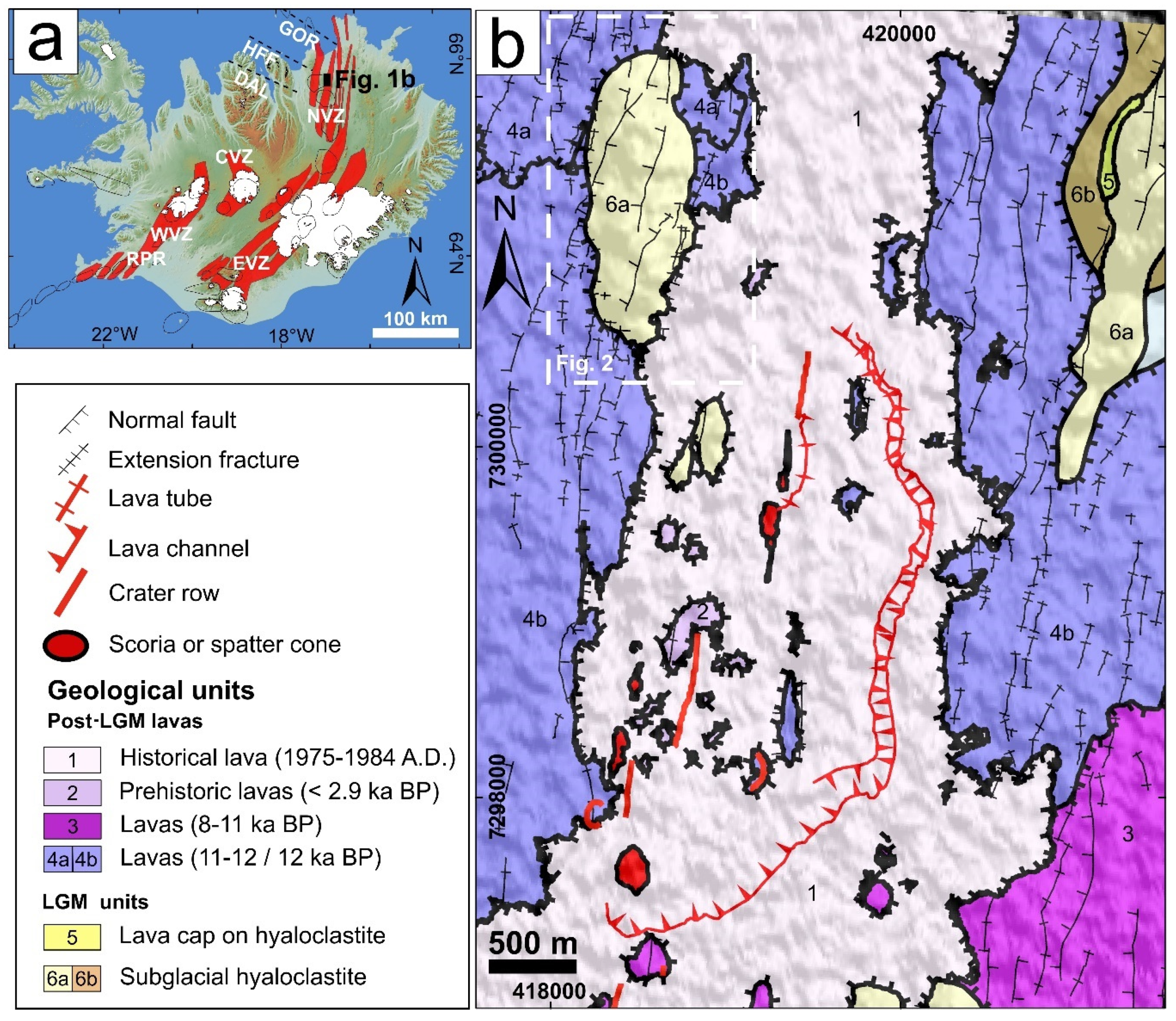
2. Geological Background

The study area is located along the 100-km long KFS, the second westernmost rift of the Northern Volcanic Zone (NVZ) (Figure 1a), which is composed of an active central volcano-caldera system, several normal faults and extension fractures, and eruptive fissures that extend mainly northward from the caldera, affecting both Pleistocene and post-Late Glacial Maximum (LGM) deposits [35,36,37], as shown in Figure 1b. All structures are mostly oriented N to NNE and have been subject to volcano-tectonic deformation for 100 thousand years [34,38]. More in detail, the study area, characterised by the presence of the Hituholar late Pleistocene hyaloclastite ridge (Figure 1b), is located 8 km north of the Krafla caldera border, along the western side of the northern KFS. The hyaloclastite deposits have been dated to the younger Weichselian [39], which in Iceland has been dated, by Radiocarbon method, more recent than 29.1–45.7 ka BP [40]. The Weichselian High Glacial, or LGM, was then reached sometime between 24.4 and 18.6 ka BP [41]. This corresponds also to the latest glacial cover of the nearby area of Melrakkasletta, which became deglaciated at 12.1 ka BP [42]. Thus, the age of the hyaloclastite deposits can be ascribed to the Weichselian High Glacial, at 29.1–12.1 ka BP. The hyaloclastite ridge, elongated N-S, is affected by several N-S to NNE-SSW-striking normal faults and extension fractures, and is surrounded by post-LGM horizontal lavas. These lavas belong to three basaltic, Holocene main sequences: the oldest two sequences are 11–12 ka old, whereas the uppermost lavas belong to the 1975–1984 AD Krafla eruptive period.
The KFS has been affected by the most recent rifting event within the NVZ [43,44], that began in December 1975 [45,46] and lasted until 1984, accompanied by about 20 rifting episodes and numerous lava flows. During each rifting episode, magma escaped from the chamber below the Krafla volcano (situated between 3 and 7 km depth [47]) and intruded northward along the fissure swarm in the form of kms-long dykes [48]. Such dykes typically propagated up to the surface in the caldera region and to a depth of about 3 km at the northern end of the KFS [49], accompanied by diffuse seismicity [50]. These repeated events caused extension of the fault and fissure swarm above the dykes, resulting in subsidence of the axial part of the swarm and uplift of the flanks, followed by viscoelastic relaxation that further contributed to the total extension [51]. The total widening across the KFS during this rifting phase ranged from 2 to 6 m, with a local maximum of 9 m [43,44]. In the successive years, GPS geodetic monitoring has shown a large, systematic, rift-normal expansion that was interpreted as post-rifting relaxation of compressional stress accumulated in the near-boundary region of the plates, as a consequence of the 1975–1984 repeated dyke intrusions [48,51,52,53]. Previous authors indicate a higher extension rate than the computed regional rate, which in north Iceland is 1.8 cm/yr [54], with a maximum rift-normal extension rate of 4.5 cm/yr near the rift, decreasing to 3 cm/yr at large distances. A more recent work [55] indicates that the current horizontal velocity field, holding North America Plate fixed, is of 2.34 ± 0.38 cm/yr in direction N106.9° E ± 8.9° in North Iceland. Further rift expansion was measured through satellite synthetic aperture radar data acquired in the years 1993–2008, which was explained by the combination of plate spreading, viscoelastic relaxation following the 1975–1984 intrusions and inflation/deflation of shallow magma chambers beneath the Krafla central volcano [56]. Another major rifting episode at KFS occurred in 1724–1729, known as ‘Mývatn fires episode’ [45]. Regarding the spreading direction in the NVZ, Drouin et al. [57] suggested a spreading direction of N112° E, based only on GPS data and for a limited time window of 4 years. Other previous works, based on GPS data and regarding two time intervals, 1997–2011 and 2006–2010, provided values of N109° E and N115° E, respectively [58,59]. Lower values of spreading direction are given from works that consider also geological data. In fact, Hjartardóttir et al. [60] provided a value of N106° E for the NVZ that is based on geomagnetic data (up to 2.6 Ma—long-term data) available in DeMets et al. [54]. The latter provided a value of N104° E for the whole Iceland, both considering GPS and geological data (magnetic, bathymetric and earthquake data; up to 3.16 Ma—long-term data). Finally, Bonali et al. [17,61] provided a range of N103–108° E, based on an extensive UAV survey and data collection in Holocene units at Theistareykir Fissure Swarm (ThFS), that is the westernmost rift of the NVZ.

3. Methods

This section is devoted to illustrating the overall methodology we adopted in this work, starting from the first steps focused on planning of UAV surveys and related photo collection, to photogrammetry processing with the aim of building the 3-D model, the orthomosaic and the DSM, and, finally, to the collection of quantitative data on the above mentioned outputs.

3.1. Drone Surveys and Data Collection

Our approach, based on the application of SfM photogrammetry techniques through drone surveys (Figure 2b), has been made possible thanks to the DJI Phantom 4 Pro (Figure 2a), a versatile quadcopter, which, according to previous studies [17,19,63], has been proved to be suitable for surveying volcanic terrains with difficult logistic conditions (e.g., outcropping lavas). This UAV is equipped with a 20 Megapixels camera and an integrated Satellite Positioning System GPS/GLONASS (referred to the WGS84 datum). Metadata of the collected images are stored in EXIF files (Exchangeable Image File Format) which include information such as shutter speed, apertures, ISO and GPS coordinates (Datum WGS84).
Before starting all UAV surveys, a reconnaissance of the selected area has been done to locate any potential terrain obstacle and to evaluate the potential flight path accordingly. After this first visual evaluation, we created a polygonal shapefile in a GIS environment covering the target area, tailored on a satellite image, and we divided it into nine subareas that covered all the features that we wanted to map: extension fractures and normal faults affecting the hyaloclastites and post-LGM lava units (Figure 1 and Figure 2c). The extension of each subarea has been defined to use a maximum of two UAV batteries for each area, considering a flight height between 80 and 95 m to reach a ground resolution of 2–3 cm for the orthomosaic. Shapefiles were converted into KML format and imported in DJI Ground Station PRO (https://www.dji.com/ground-station-pro), a free iPad app for DJI drones operations. This app allowed to generate nine different missions and to define and change for each of them the flight path direction, the flight height, as well as to fix camera parameters and directly check data acquisition on the iPad display. In fact, for all the surveys, fixed acquisition parameters were set (Table 1) to obtain proper images alignment and to reduce the distortions on the resulting models: (i) The overlap has been slightly decreased, with respect to previous authors [17,64,65,66,67], to 85% along the path and 80% in lateral direction, in order to save time during each flight mission; (ii) photos have been captured using equal time interval mode and using constant velocity [17,68]: these two parameters are automatically managed by DJI Ground Station PRO in order to guarantee the set-up photos overlap at the given flight height. Additionally, a series of environmental conditions have been taken into account: for example, the sun orientation, which is the same for all surveys (sun to the zenith) since they have been performed in time sequence, and the light conditions, which were always optimal and suitable for the camera ISO range (100–1600). Also, we considered the wind speed and direction, being always parallel to the main and longer paths during each drone survey, and we maintained a constant path direction in each subarea in order to be sure to obtain the entire coverage of the whole big area.
Furthermore, a crucial step in order to georeference the resulting models (orthomosaics and DSMs) and thus to allow the collection of high-precision quantitative measurements, was to collect World Geodetic System (WGS84) coordinates of ground control points (GCPs) in each drone-surveyed area. The placement and acquisition of GCPs was planned considering the specificities of the study area. We collected 37 GCPs (Figure 2c) distributed both at the corners and in the central part of each subarea to reduce the doming effect resulting from SfM processing and reduce systematic error [69,70,71,72]. Such GCPs can be artificial or natural objects, both must be easily recognizable on drone-captured photos (Figure 3). Artificial GCPs deployment and recovery, on an extensive area, is really time-consuming since targets must be placed before starting the survey and retrieved afterward. For this reason, we used both artificial and natural targets as GCPs: artificial targets include objects with bright colours (e.g., Figure 3b), the corner of the backpack case of our drone (Figure 3c), and series of slices of white bread arranged to form an X on the ground (Figure 3d), whereas natural targets include massive rocks with defined geometric shapes (e.g., Figure 3e) and geometric lava flow margins (e.g., Figure 3f). Slices of white bread and natural targets were easily recognisable from UAV images and they have been used since the unnecessity to retrieve them could significantly speed up the survey.
The collection of GCPs has been performed with the Emlid Reach RS© single frequency receivers in RTK configuration (with centimetre-level accuracy), linked in real time by NTRIP to the Icelandic CORS network (ICECORS—https://www.lmi.is/en/icecors-network/), used as reference station. Because of the use of RTK/GNSS GPS information, we expect to obtain a model with centimetric accuracy, as already highlighted by several authors; for a more in-depth reading about the resulting accuracy we suggest the work proposed by the following authors: [73,74,75,76].

3.2. Photogrammetry Processing

UAV images have been processed using Agisoft METASHAPE (http://www.agisoft.com/), a commercial SfM software, and Agisoft Cloud beta service for data processing. The software was chosen for its user-friendly interface, spontaneous workflow, the good quality of the outputs [77,78,79] and the reasonable price of the educational license. These qualities have made it a broadly used application by the earth science community. SfM photogrammetric workflow, described in detail by [80,81], consists in a sequence of steps that from a set of overlapping images lead to the creation of a sparse and dense cloud, a 3-D tiled model, an orthomosaic and a DSM as final products (Table 2).
The processing approach can be divided into four main stages:
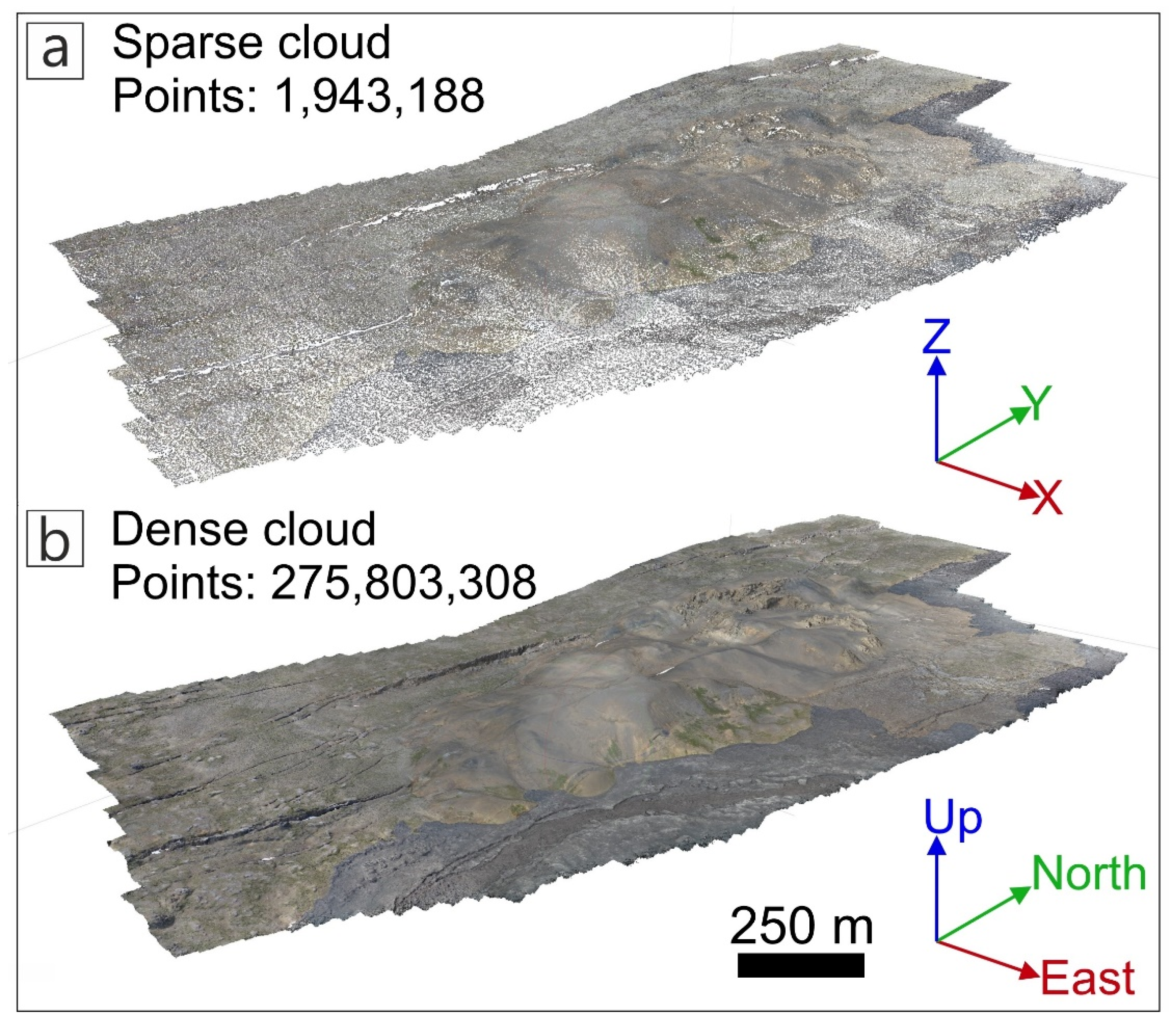
  • Photo alignment: an initial low-quality photo alignment using common key points in each image generated a sparse 3-D point cloud (Figure 4a). The focal length and photo dimensions were automatically computed by the software and then used for the subsequent calibration of the core parameters of the camera (principal point coordinates, lens distortion coefficients).
  • Georeferencing: GCPs were identified into the photos and markers have been assigned with the surveyed coordinates. This process allowed to scale and georeference the point cloud and thus to improve the accuracy of the final models. Then, the images were realigned using high accuracy settings and default values for Tie and Key points settings, 40,000 and 4000 respectively, and using Generic and Reference preselection settings.
  • Dense Point Cloud Building: a 3-D dense point cloud was generated, using a mild depth filtering and medium quality settings, from the sparse point cloud (Figure 4b).
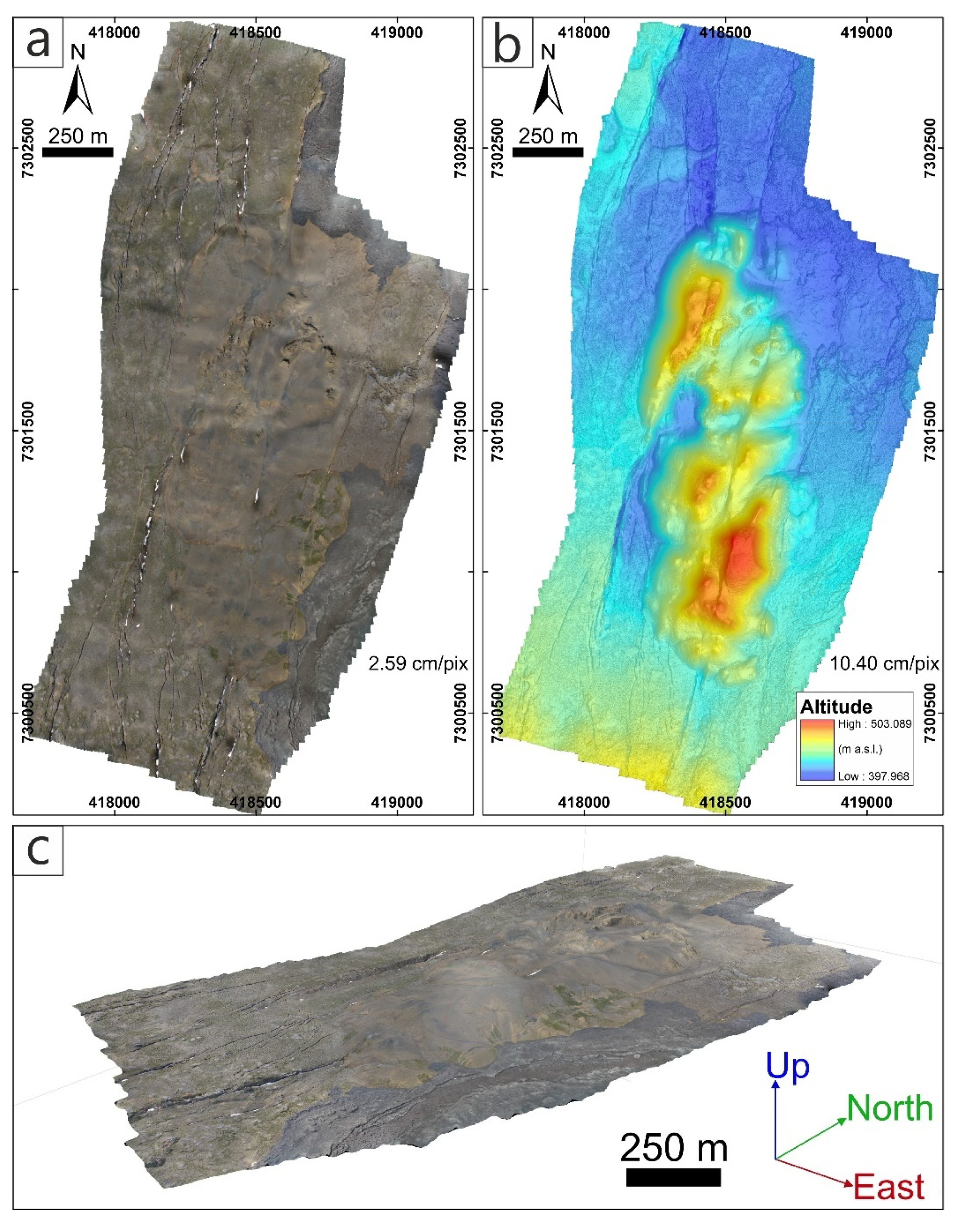
  • DSM and orthomosaic generation: a DSM was generated from the dense point cloud, and successively the orthomosaic was produced using the corresponding DSM (Figure 5a,b).
  • The software also allows to generate a high-quality 3-D tiled model, both including the mesh and the texture (Figure 5c). The latter can be used as a scenario for immersive virtual reality [31]; here we suggest a Medium quality set-up with a tile size of 4096 × 4096 pixels.
All outputs refer to the geographic coordinate system (WGS84).

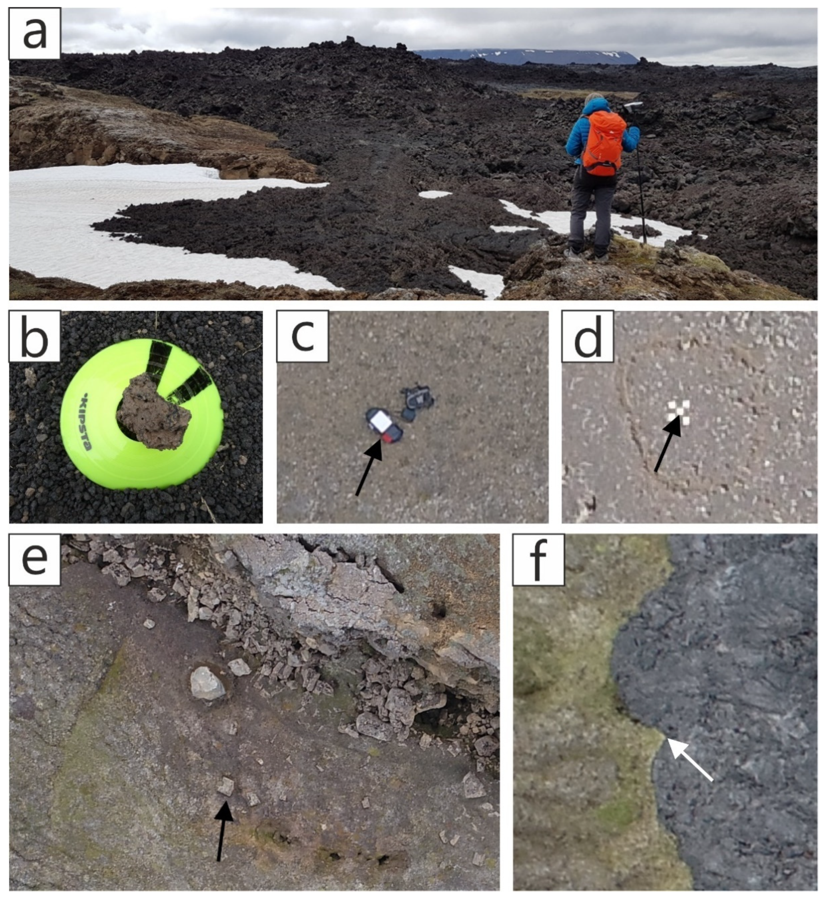
3.3. Data Collection on 2-D and 3-D Outputs

Once the resulting models had been processed, we imported the DSM and the orthomosaic in a GIS environment and mapped all fractures in the area, and remapped all post-LGM and LGM stratigraphic units (Figure 6a): these steps have been made possible thanks to the very high-resolution of the orthomosaic. Fractures have been further classified as normal faults when associated with a continuous and appreciable, and persistent, vertical offset > 0.5 m, calculated on the DSM, whereas they have been classified as extension fractures when associated with vertical offset less than 0.5 m. Apart from the DSM, the use of the 3-D tiled model, that can be defined as a virtual outcrop [82,83], has been crucial in order to perform visual checks in key points of each examined structure. Such models can be used for observation using an immersive virtual reality [31,64,65,84] and non-immersive virtual reality [85] approach as well as 3-D visualisation on a computer workstation [82].
Different types of quantitative data have been taken: along normal faults, we quantified the strike and the vertical offset, by measuring differences in altitude along 50-m-spaced topographic profiles traced on the DSM, orthogonally to the fault scarp, whereas along extension fractures we collected the strike, the amount of dilation and opening direction values. More in detail, wherever piercing points on each side of the extension fractures were clearly visible, we traced a line connecting them on the orthomosaic, and we calculated its strike and length to obtain the direction and the amount of opening, respectively. All factors that could alter the accuracy of the resulting values have been avoided, by making sure to collect data only at fractures not affected by erosion and sedimentation, without falling rocks on their sides and far away from fault rims to avoid local gravity effects. For these quantitative measurements, we also used the SfM-derived 3-D model for some checks to better recognize all fault scarps and visualize piercing points. Finally, all collected data have been used for two aims: defining the spreading direction in the area and quantifying the overall extension rate during late Pleistocene and Holocene times. We calculated all horizontal dilation values along N105° E-trending transects, in order to obtain the cumulative dilation, stretch, and extension rate in the two main outcropping successions (LGM and post-LGM). These transects have been located in order to cover both the LGM unit and the post-LGM units. The N105° E is the mean value of the spreading direction given by DeMets et al. [54] and Hjartardóttir et al. [60], both considering geological data for a long-term time window.

4. Results

4.1. High Resolution Outputs from Photogrammetry Processing

The areal coverage of our study area is about 2.7 km2 subdivided into nine different surveys, performed at 80–95 m of height from the ground; the surveys were carried out during the summer 2019 campaign, during which we collected a total of 6068 photos during a total flight time of 4.68 hrs. Because of the above described workflow, such photos were used to reconstruct a high quality orthomosaic and a DSM (Figure 5a,b), respectively characterized by a resolution of 2.59 and 10.40 cm/pixel; the resulting GeoTIFFs have a storage dimension of 15.8 and 1.11 GBs respectively, the orthomosaic has been converted to JPEG 2000 (JP2) for data collection in GIS. The 3-D tiled model is characterised by a texture resolution that is identical to the orthomosaic and a storage dimension of 9.87 GBs. Regarding the processing time, as detailed in Table 2, all outputs have been generated in 46.8 h, where the most time-consuming processing have been the dense cloud and 3-D tiled model generation.

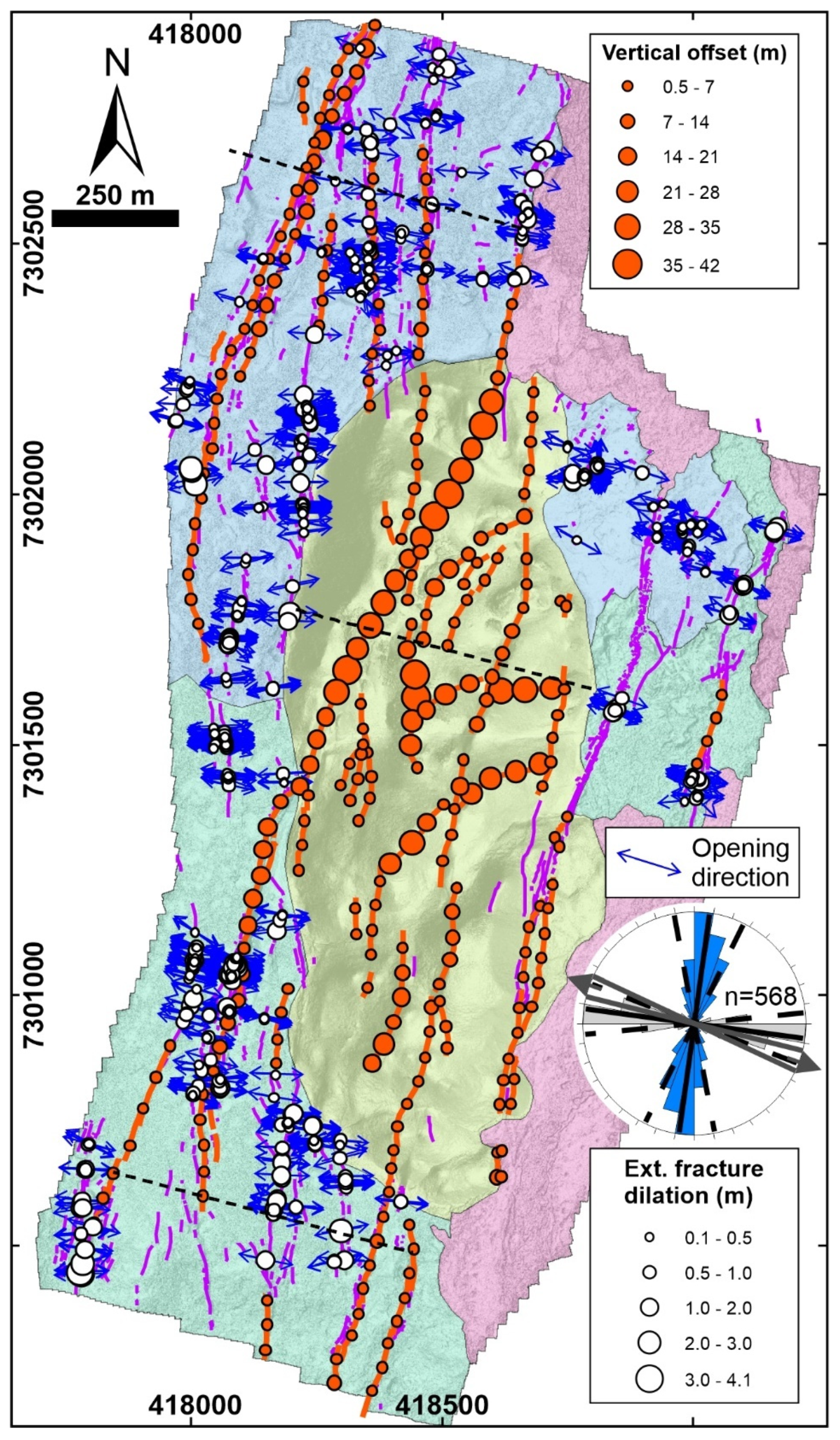
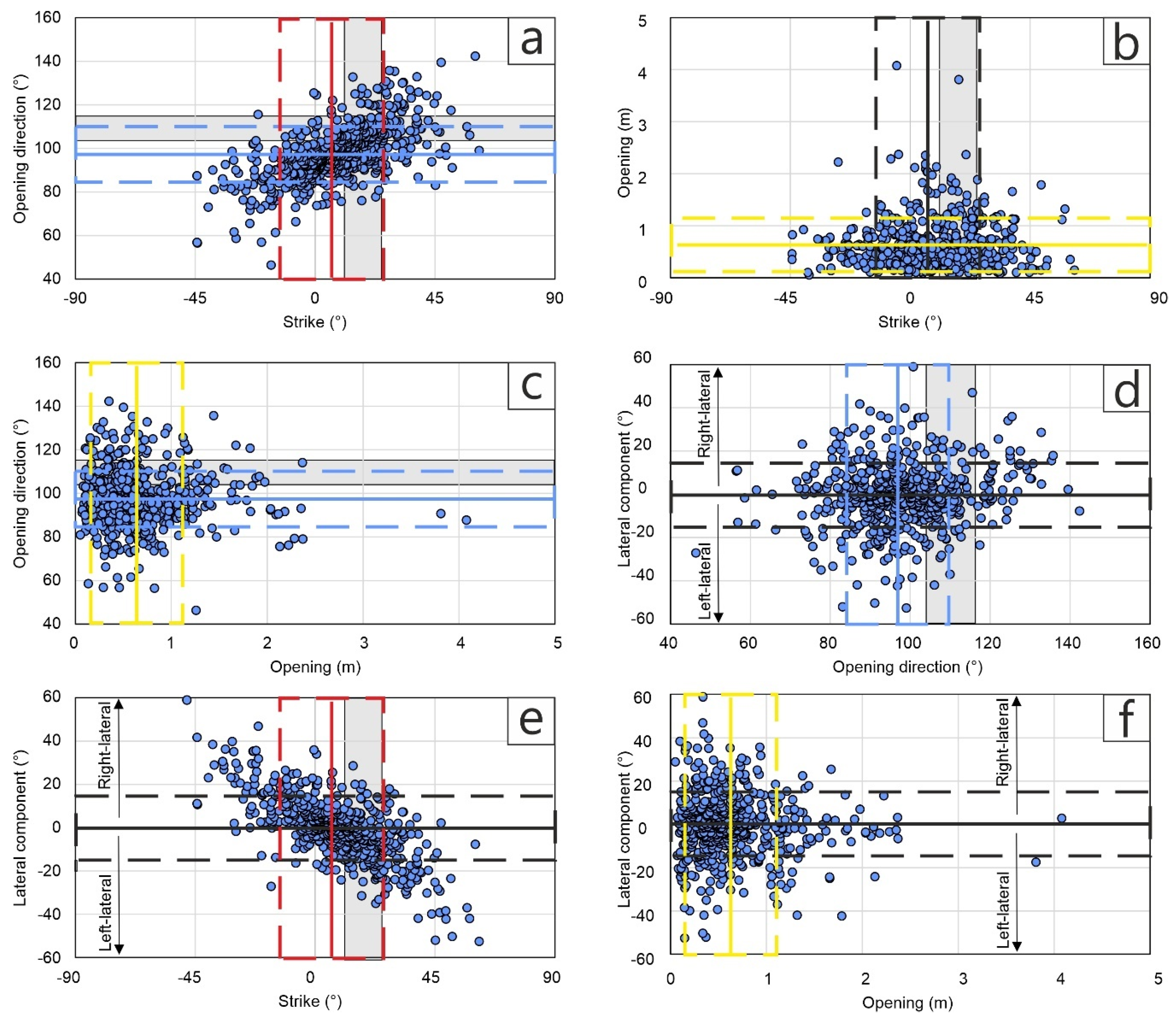
4.2. New Geological-Structural Data

During the present work, we mapped a total of 1355 fractures classified as normal faults (86) and extension fractures (1269): these structures strike from NNW-SSE to NE-SW, but are mostly in the range N0–20° E, whereby the av. strike is N8.2° E, as shown in the rose diagram in Figure 6b. The longest fracture reaches a length of 1156.1 m, whereas the overall av. length is 28.3 m (Figure 6e). Although the whole Krafla rift has an about N-S elongation, once you define the structures in detail it emerges that several single faults have a bimodal strike given mostly by N-S and NNE-SSW segments, with a curvilinear trace in plan view.
Owing to the high resolution of the new DSM and orthomosaic, the number of mapped fractures is dramatically greater with respect to the 45 main fractures documented on the 1:100,000 scale geological map [39] (Figure 1b). In addition to the newly mapped fractures mentioned above, we have also redrawn the geological map of the area, tracing with very high detail the geological limits, as shown in Figure 6a and Figure 7.
In regard to normal faults, they mainly strike from N-S to NE-SW, dipping towards WNW and ESE (Figure 6c), and show an overall av. and maximum length of 167.9 m and 1156.1 m respectively (Figure 6e). On the other hand, extension fractures mainly strike from NNW to NNE, with an av. value of N8.1° E (Figure 6d), and an overall av. and maximum length of 18.8 m and 240.7 m respectively (Figure 6e). In order to better define the deformation processes that have been occurring since late Pleistocene times, we collected a series of quantitative data at a total of 852 sites, 284 along normal faults and 568 along extension fractures. Regarding normal faults, we collected 284 vertical offsets, thus obtaining a maximum value of 42 m along faults affecting LGM units and of 19 m along faults affecting post-LGM units (Figure 7). Regarding extension fractures, we collected a total of 1704 structural data, consisting of strike, opening direction and fracture dilation, at 568 different sites (Figure 7): all these data have been collected in the post-LGM units (no extension fractures in historical lavas or in LGM units).
Opening direction values are in the range N46.3–142.3° E, with a mean value of N97.7° E and a SD of 13.3°: only 109 values fall within the spreading direction range (N104–115° E), which is based on spreading direction estimates given in the literature for the NVZ [17,54,57,58,59,60,61]. We also measured the extension fracture azimuth that ranges N48.1° W–N61.5° E, with a mean value of N7.9° E and a SD of 18.5°: only 119 values show an azimuth that is compatible with the spreading direction range. If we consider both the extension fractures opening direction and strike, only 43 out of 568 are compatible with the spreading direction range N104–115° E (Figure 8a).
The dilation is in the range of 0.1–4.1 m, with a mean value of 0.64 m and a SD of 0.5 m. Figure 8b shows the relation between fractures strike and amount of opening: we observe that most of extension fractures with a dilation > 1 m have a strike between NNW-SSE and NE-SW, and the wider fractures are characterized by an opening direction N80–120° E (Figure 8c) and a lateral component < (+/−) 20° (Figure 8f). The greatest amount of opening (4.1 m) is found in correspondence of opening direction values of N87.8° E and with a very low value of lateral component.
Regarding the presence of lateral components of motion along extension fractures, 358 exceed 5° of lateral component, 177 of which are right-lateral and 181 left-lateral with an av. lateral component of 15° and 16°, respectively; the overall av. value is 0.29°, the maximum value is 46.9°, corresponding to a right-lateral component (Figure 8d).
On the other hand, by increasing the extension fractures strike, we observe an increase in opening directions with a sort of clockwise rotation of values (Figure 8a). In fact, considering N-S to NE-SW fractures, opening direction values range from N73.7° E to N142.3° E, whereas NW-SE fractures are characterized by opening direction values ranging from N46.4° E to N125.5° E. On the other hand, by increasing the fracture strike, we notice a decrease in the lateral component, that changes from right-lateral to left-lateral (Figure 8e). Finally, values of the amount of opening slightly increase for fractures characterized by a lower component of motion (Figure 8f).
We also measured the extensional strain in the area by cumulating the dilation values obtained at both extension fractures and normal faults, along three N105° E-striking transects, each with a length of 0.62 km (Figure 7). To calculate the dilatational component at normal faults, we used the measured vertical offset, considering a dip of the fault plane of 70° [86]. Along the northernmost transect, which cuts structures affecting 11–12 ka BP lavas, we measured a cumulated dilation of 16.6 m, corresponding to a stretch of 1.027; along the central one, which cuts only faults affecting the hyaloclastites, we obtained a cumulated dilation of 29.3 m, corresponding to a stretch value of 1.049; along the southernmost transect, which cuts structures affecting 12 ka lavas, the cumulated dilation has a value of 11.2 m, with a stretch value of 1.018. The overall dilation, calculated in the central part of the area along a 1.23 km-long transect and considering all fractures affecting LGM and post-LGM units, is 36.4 m, corresponding to a stretch of 1.0304.

5. Discussion

5.1. Rift Architecture and Kinematics

The studied rift segment is located along the north-western part of the KFS and is characterised by the presence of grabens arranged en-échelon with a left-stepping geometry. In the study area, two main grabens are present: one, to the north, affects the Holocene lavas only, and disappears in correspondence of the other graben. This second graben is located further south and affects mostly the hyaloclastic ridge and, to a lesser extent, prolongs into the surrounding Holocene lava succession.
The southern graben is a few tens of meters wide at its northern and southern terminations, whereas its width increases up to 300 m in its central part. This geometry in plan view cannot be related to the presence of the volcanic ridge respect to the surrounding flat area for two reasons: (i) Classical studies showed that the presence of a volcanic edifice strongly influences fault orientation by deflecting and converging faults that tend to become radial at the cone, assuming an hourglass pattern [87,88]; in our case instead, faults tend to diverge in correspondence of the ridge. (ii) In plan view, inclined normal faults tend to diverge in correspondence of a topographic high, like a volcanic cone, but in our case it is possible to observe that faults diverge and graben width increases to the north exactly in correspondence of the contact between the hyaloclastites and the lava flows, and to the south in the flat area occupied by the lavas. Moreover, the difference in altitude between the ridge and the surrounding flat area is modest and cannot account for the bulge of fault traces as simply because of fault outcrop following topography. We propose that the increase of graben width in correspondence of the hyaloclastite ridge could instead be related to the mechanical contact between the stiffer lava succession and the softer hyaloclastites: the rheological contrast between the two rock units leads to faults that tend to follow the outline of the contact, favouring concentric faults. This is similar to what has been noticed after simulating a magma chamber and diffuse rift extension [88]: in this case, the presence of a magma chamber affects the faults orientation that close to the intrusion edge change their direction, mimicking the intrusion shape by curving around it.
Focusing on the kinematics of extension fractures, the collected data suggest an av. spreading direction of N97.7° E, with a range of N46.3–142.3° E for the Holocene times (Figure 7). This av. value is lower than those given in the literature that range between N104° E and N115° E [54,57,58,59,60]. The av. spreading value calculated in the present research is closer to those that take into account geological data that cover a larger time window [17,54,60,61]) with respect to only GPS data [57,58,59], suggesting a slight overall anticlockwise rotation of the spreading direction in the NW part of the Krafla rift.
The overall fracture azimuth is suggested to be orthogonal to the spreading vector range discussed in the above section: in fact, longer and more developed fractures show an azimuth N-S to NNE-SSW (Figure 6a,b,e), as suggested for the active Krafla fissure swarm [60].
Finally, we paid attention to the presence of strike-slip components along the extension fractures, where the av. value suggests an overall very limited left-lateral component, even though the majority of data are characterized by values with right-lateral components (Figure 8e,f). We believe that this component is the result of local perturbations by dyking at shallow depths, as shown for the 2014–2015 Bárðarbunga dyking event [89] and as suggested in the ThFS [16,17]. In support of this hypothesis, the area has been subjected to recent historical rifting events characterized by N-propagating dykes [48], and Tibaldi et al. [37] described textbook examples of dyke-induced deformation at the surface in the eastern part of the area presented in this study.

5.2. Rift Extension Rate

The total extension measured along the fractures cropping out in the Holocene lava succession is, along two transects, 16.6 m and 11.2 m, whereas the total extension in the hyaloclastites is 29.3 m, coherently with the older stratigraphic age of the latter. Assuming the age of 11.5 ± 0.5 ka BP for the post-LGM lava units, and of 20.6 ± 8.5 ka BP for the hyaloclastite deposits, we obtain an extension rate of 1.4 ± 0.7 mm/yr and 1.7 ± 0.7 mm/yr, respectively. Our measured extension rates of 1.4 mm/yr and 1.7 ± 0.7 mm/yr for the shorter and longer periods are coherent with each other, but much slower than the GPS velocity field measured after the 1975–1984 rifting/dyking period (3–4.5 cm/yr). We thus consider that our measures do represent the real long-term deformation field of the western part of the Krafla rift. This represents only a fraction of the total extension that characterizes this rift, which in turn is a fraction of the extension of the whole NVZ of 1.8–2.3 cm/yr [54,55]. From another point of view, focusing on the amount of horizontal dilation, the stretch in the area is 1.018–1.027 for post-LGM units, 1.049 for LGM unit and is 1.030 if we consider both. In the Krafla area, a stretch value of 1.009 was previously calculated [90] along a 30-m-long transect in an area located just north of the 1984 Krafla lava flow, totalling a horizontal dilation of 30 m for the last 10,000 yrs. Even though, owing to the high resolution of our SfM-derived models, we collected a larger number of data, also at fractures with centimetric dilation, we think that both values describe the contribution of both tectonic and magmatic forces (dyke intrusion) in dictating deformation at the surface in terms of extension fractures opening and normal faulting. Differently, Paquet et al. [91] calculated a stretch ratio of 1.036–1.046 across the Tertiary Alftafjordur dyke swarm, describing the deformation that lasted 1 Ma or more. The stretch value that we calculated on the LGM units resulted like Paquet et al. [91], even though they considered a much longer time span and a greater depth of analysis since they studied an ancient rift zone exposed by glacial erosion. We finally suggest that a stretch value <1.030 can be considered as representative of the influence of both tectonic and magmatic forces; on the contrary, based on data from the present work and from [91], any classification for stretch values >1.030 is controversial and must be subject to further research.

5.3. Methodological Aspects

Even though the application of the method can have some limitations (e.g., the age of structures should be kind of ‘recent’, the research area should be well exposed with a low vegetation coverage, basic geological researches should be completed ahead of the survey), our work confirms the usefulness of the UAV-based SfM as a support for classical fieldwork to collect massive amounts of high resolution quantitative data, here aimed at reconstructing late Pleistocene-Holocene deformation in an active volcano-tectonic region, being here a key area within the active Krafla rift. At a general level, the use of UAVs in geoscience has increased over the past decade [92,93,94,95,96,97,98,99,100,101]. The affordability of such method is one of the main reasons why the geosciences community broadly adopts it: UAV data acquisition represents, in fact, a less expensive alternative to other techniques, such as Terrestrial Laser Scanning (TLS), Airborne Laser Scanning (ALS) and LiDAR [102,103]. Another reason for which this methodology has been broadly used is the possibility to save time with respect to fieldwork, especially in vast areas and along structures that can be tens of km long [15,104], and to enable to reach key geological sites that are generally inaccessible because of hard logistic conditions, like volcano edifices affected by caldera or lateral collapse [105,106,107]. Furthermore, the rapidity of data capturing, the quick processing and the high accuracy of the output model generated through the UAV-SfM technique allow to observe at a centimetric detail the characteristics of the ground surface and outcrops, for example by catching also micro-topographic variations. As an example of the great amount of measurements that can be collected through this method, Bonali et al. [17] were able to collect 1098 measurements at 387 sites in a volcano-tectonic field, comprising azimuth, dilation and opening direction of extension fractures by using a commercial-grade UAV and applying SfM algorithms, thus providing a contribution to the reconstruction of the tectonic evolution in such an active rift zone in NE Iceland.
Another advantage of this methodology is represented by the continuous improvements over the years of the consumer-grade UAVs, in terms of flight stability, battery capacity and camera quality, owing to the constant release of new products: for example, in this work we used the DJI Phantom 4 Pro (20 Megapixel and ISO range 100–12800), which has been released less than a year later with respect to the DJI Phantom 4 (12 Megapixel and ISO range 100–1600). This implies that in the next years, owing to such fast improvements of the UAV technology, geological studies will achieve better quality by flying at a higher altitude and covering a wider area. Finally, the SfM technique could be applied with a low-cost workflow, particularly suitable for field research, which allows any user to process the data [108].
Through a methodological point of view, we tested two novelties in our approach: (i) we slightly decreased the image overlap to save time during each single flight mission. This overlap decrease resulted in 30% of saved time. Considering our overall survey, we saved about 2 h, which is plenty of time in areas usually affected by wind and rain. (ii) We mainly used natural, ecological, or already available artificial targets for GCPs collection, this action halved the time usually necessary for this fundamental task. We obtained excellent models as output where we collected very high-resolution structural data, especially regarding piercing points along extension fractures. Of course, both novelties can be applied to further researches and areas. In addition, the area of this research is characterized by an overall morphology that is more complicated than in Bonali et al. [17]: in fact normal faults have a different morphological expression due to the age and characteristics of volcanic units. Finally, the presence of the Hituholar volcanic edifice, with an elevation of more than 100 m from the surrounding area, has made it more challenging to plan and execute UAV missions. Even so, we reached excellent resolution and accuracy in all SfM outputs, allowing us to collect all data necessary to define spreading direction and stretch in the studied area, enhancing the importance of this methodology in this kind of studies.
The UAV-based SfM also presents a few limitations, such as the dependence on the battery life/flight time, weather conditions and legal flight restrictions. Also the necessity of positioning some GCPs, in order to reference the model accurately, could be time spending and thus could slow down the survey, especially over vast areas. Smith et al. [109] recommended the use of at least 3 GCPs; other authors used a higher number of GCPs (up to 95 across a 100 m grid), but reducing the image overlap to 60–70% [110]. With a greater overlap, on the other hand, a lesser number of GCPs can be used [68,111]. The number of GCPs can also be reduced if the geometry network results sufficiently strong [72] or by using an UAV incorporating onboard RTK-GNSS sensors that would allow to generate models with centimetric spatial accuracy without placing GCPs.
In our work, we used 37 GCPs, both along the corners and at the centre of every area, in order to reduce the ‘doming’ effect and reduce systematic errors [69,70,71,72]. Another strategy to reduce the ‘doming’ effect on the resulting DTM/DSM [73], consists of collecting aerial photos with an oblique inclination with respect to the ground [112]. Nevertheless, this strategy results in greater consumption of the battery power and so it is useless for commercial UAVs equipped with low-cost GPS chipset, where GCPs collection is crucial to georeference the model; it is thus more efficient to design a GCPs survey as proposed in the present work.
We thus selected our flight strategy to reach a good compromise between battery consumption, survey time, area extension, data resolution and accuracy of the models. In just two days of fieldwork and almost 46 h of processing of about 7000 UAV pictures, we mapped an area of 232 Ha (2.3 km2). Moreover, the achieved resolution of the orthomosaic (2.6 cm/px) and the DSM (10 cm/px) resulted sufficiently detailed for surveying extension fractures and collecting plenty of data of opening vectors, down to centimetric values of dilation. This high accuracy opens the possibility to carry out repeated UAV surveys across the same area at regular time intervals, in order to study the present-day deformation and observe its evolution over time. This could be applied, for example in the KFS, by comparing the resulting models (orthomosaics and DSMs) before and after a rifting event, if the superficial deformation is larger than the model resolution. Regardless, additional improvements are suggested to define the most efficient survey approach for DSMs reconstruction, mainly devoted to measuring vertical offset at normal faults. The fast evolution of UAVs, equipped with RTK positioning system, can represent a solution for the above-presented limitations, increasing the accuracy of the model, flying also at greater heights. Finally, the resulting 3-D models can be navigated in the immersive virtual reality, useful both for scientific research and teaching and divulgation purposes [17,31,64,65].

6. Conclusions

We used drone surveys coupled with structure-from-motion photogrammetry, introducing two novelties to increase the efficiency of drone surveys, to analyse a remote area characterised by rough terrains in the NW part of the KFS (NE Iceland). This is a volcanotectonic rift composed of eruptive centres and N-S to NNE-SSW fissures and normal faults. The central part of the surveyed sector has a hyaloclastite ridge composed of deposits dated, on a stratigraphic basis, to the Weichselian High Glacial (LGM here dated 29.1–12.1 ka BP). These are surrounded by a series of flat lava flows dated at 11–12 ka BP, and locally by 1975–1984 AD lavas.
The integration of the data enabled us to recognize that this segment of the KFS is made of grabens arranged en-échelon with a left-stepping geometry. A major graben increases in width in correspondence of the hyaloclastite ridge; we interpret this geometry as resulting from the mechanical contrast between the stiffer lava succession and the softer hyaloclastites, which favours the development of concentric faults.
The direction of extension has also been measured at hundreds of sites, resulting in an E-W to WNW-ESE trend, normal to the fissure and fault strikes. The total extension results to be 16.6 and 11.2 m along the faults and fissures cropping out in the Holocene lava succession, whereas the total extension measured in the hyaloclastites is 29.3 m. This indicates an extension rate of 1.4 mm/yr in the Holocene lavas and 1.7 ± 0.7 mm/yr in the latest Pleistocene hyaloclastite deposits. We consider these data to represent the real values of long-term extension in this part of the Northern Volcanic Zone, much slower than the GPS velocity field measured around the Krafla system that resulted from the 1975–1984 rifting and dyking events. The av. spreading direction here quantified is N97.7° E.

Author Contributions

Writing—original draft, F.L.B., A.T., N.C., L.F. and E.R. All authors have read and agreed to the published version of the manuscript.

Funding

This research received no external funding.

Acknowledgments

Three anonymous reviewers are acknowledged for their useful comments on an early version of the manuscript. This study has been conducted in the framework of the International Lithosphere Program—Task Force II (Leader A. Tibaldi) and of the European Space Agency project n. 38829 (Leader F. L. Bonali). This article is also an outcome of Project MIUR—Dipartimenti di Eccellenza 2018–2022. Agisoft Metashape is acknowledged for photogrammetric data processing. Finally, this paper is an outcome of GeoVires, the Virtual Reality Lab for Earth Sciences host at Department of Earth and Environmental Sciences, University of Milan Bicocca, U4, Piazza della Scienza 4, 20126 Milan, Italy—https://geovires.unimib.it/.

Conflicts of Interest

The authors declare no conflict of interest.

Abbreviations

CORSContinuously Operating Reference Station
CVZCentral Volcanic Zone
DSMDigital Surface Model
DTMDigital Terrain Model
EVZEast Volcanic Zone
EXIFExchangeable Image File Format
GISGeographic Information System
GLONASSGLObal NAvigation Satellite System
GPSGlobal Positioning System
GCPGround Control Point
GNSSGlobal Navigation Satellite System
KFSKrafla Fissure Swarm
ICECORSRegional positioning service of Iceland
LGMLate Glacial Maximum
LiDARLight Detection and Ranging/Laser Imaging Detection and Ranging
NTRIPNetworked Transport of RTCM via Internet Protocol
NVZNorthern Volcanic Zone
RTKReal-time kinematic
SfMStructure-from-Motion
TLSTerrestrial Laser Scanning
ALSAirborne Laser Scanning
ThFSTheistareykir Fissure Swarm
UAVUnmanned Aerial Vehicles
UTMUniversal Transverse Mercator
WGS84World Geodetic System 1984
WVZWestern Volcanic Zone

References

  1. Lyakhovsky, V.; Segev, A.; Schattner, U.; Weinberger, R. Deformation and seismicity associated with continental rift zones propagating toward continental margins. Geochem. Geophys. Geosyst. 2012, 13, Q01012. [Google Scholar] [CrossRef]
  2. Keir, D.; Ebinger, C.J.; Stuart, G.W.; Daly, E.; Ayele, A. Strain accommodation by magmatism and faulting as rifting proceeds to breakup: Seismicity of the northern Ethiopian rift. J. Geophys. Res. Solid Earth 2006, 111, B05314. [Google Scholar] [CrossRef]
  3. Jestin, F.; Huchon, P.; Gaulier, J.M. The Somalia plate and the East-African Rift system—Present-day kinematics. Geophys. J. Int. 1994, 116, 637–654. [Google Scholar] [CrossRef] [Green Version]
  4. Chu, D.; Gordon, R.G. Evidence for motion between Nubia and Somalia along the Southwest Indian Ridge. Nature 1999, 398, 64–67. [Google Scholar] [CrossRef]
  5. Tibaldi, A.; Bonali, F.L.; Mariotto, F.P.; Russo, E.; Tenti, L.R. The development of divergent margins: Insights from the North Volcanic Zone, Iceland. Earth Planet. Sci. Lett. 2019, 509, 1–8. [Google Scholar] [CrossRef]
  6. Manighetti, I.; King, G.C.P.; Gaudemer, Y.; Scholz, C.H.; Doubre, C. Slip accumulation and lateral propagation of active normal faults in Afar. J. Geophys. Res. Solid Earth 2001, 106, 13667–13696. [Google Scholar] [CrossRef]
  7. King, G.; Sammis, C.G. The role of off-fault damage in the evolution of normal faults. Earth Planet. Sci. Lett. 2004, 217, 399–408. [Google Scholar]
  8. Muraoka, H.; Kamata, H. Displacement distribution along minor fault traces. J. Struct. Geol. 1983, 5, 483–495. [Google Scholar] [CrossRef]
  9. Peacock, D.C.P.; Sanderson, D.J. Displacements, segment linkage and relay ramps in normal fault zones. J. Struct. Geol. 1991, 13, 721–733. [Google Scholar] [CrossRef]
  10. Bürgmann, R.; Pollard, D.D.; Martel, S.J. Slip distributions on faults: Effects of stress gradients, inelastic deformation, heterogeneous host-rock stiffness, and fault interaction. J. Struct. Geol. 1994, 16, 1675–1690. [Google Scholar] [CrossRef]
  11. Nicol, A.; Watterson, J.; Walsh, J.J.; Childs, C. The shapes, major axis orientations and displacement patterns of fault surfaces. J. Struct. Geol. 1996, 18, 235–248. [Google Scholar] [CrossRef]
  12. Roche, V.; Homberg, C.; Rocher, M. Fault displacement profiles in multilayer systems: From fault restriction to fault propagation. Terra Nova 2012, 24, 499–504. [Google Scholar] [CrossRef]
  13. Tibaldi, A.; Bonali, F.L.; Pasquaré Mariotto, F.A. Interaction between transform faults and rift systems: A combined field and experimental approach. Front. Earth Sci. 2016, 4, 33–47. [Google Scholar] [CrossRef] [Green Version]
  14. Dumont, S.; Klinger, Y.; Socquet, A.; Doubre, C.; Jacques, E. Magma influence on propagation of normal faults: Evidence from cumulative slip profiles along Dabbahu-Manda-Hararo rift segment (Afar, Ethiopia). J. Struct. Geol. 2017, 95, 48–59. [Google Scholar] [CrossRef] [Green Version]
  15. Pasquaré Mariotto, F.A.; Bonali, F.L.; Tibaldi, A.; Rust, D.; Oppizzi, P.; Cavallo, A. Holocene displacement field at an emerged oceanic transform-ridge junction: The Husavik-Flatey Fault-Gudfinnugja Fault system, North Iceland. J. Struct. Geol. 2015, 75, 118–134. [Google Scholar] [CrossRef] [Green Version]
  16. Bonali, F.L.; Tibaldi, A.; Mariotto, F.P.; Saviano, D.; Meloni, A.; Sajovitz, P. Geometry, oblique kinematics and extensional strain variation along a diverging plate boundary: The example of the northern Theistareykir Fissure Swarm, NE Iceland. Tectonophysics 2019, 756, 57–72. [Google Scholar] [CrossRef]
  17. Bonali, F.L.; Tibaldi, A.; Marchese, F.; Fallati, L.; Russo, E.; Corselli, C.; Savini, A. UAV-based surveying in volcano-tectonics: An example from the Iceland rift. J. Struct. Geol. 2019, 121, 46–64. [Google Scholar] [CrossRef]
  18. Bonali, F.L.; Tibaldi, A.; Mariotto, F.P.; Russo, E. Interplay between inherited rift faults and strike-slip structures: Insights from analogue models and field data from Iceland. Glob. Planet. Change 2018, 171, 88–109. [Google Scholar] [CrossRef]
  19. De Beni, E.; Cantarero, M.; Messina, A. UAVs for volcano monitoring: A new approach applied on an active lava flow on Mt. Etna (Italy), during the 27 February–02 March 2017 eruption. J. Volcanol. Geotherm. Res. 2019, 369, 250–262. [Google Scholar] [CrossRef]
  20. Johnson, K.; Nissen, E.; Saripalli, S.; Arrowsmith, J.R.; McGarey, P.; Scharer, K.; Williams, P.; Blisniuk, K. Rapid mapping of ultrafine fault zone topography with structure from motion. Geosphere 2014, 10, 969–986. [Google Scholar] [CrossRef]
  21. Angster, S.; Wesnousky, S.; Huang, W.L.; Kent, G.; Nakata, T.; Goto, H. Application of UAV photography to refining the slip rate on the Pyramid Lake fault zone, Nevada. Bull. Seismol. Soc. Am. 2016, 106, 785–798. [Google Scholar] [CrossRef] [Green Version]
  22. Deffontaines, B.; Chang, K.J.; Champenois, J.; Fruneau, B.; Pathier, E.; Hu, J.C.; Lu, S.T.; Liu, Y.C. Active interseismic shallow deformation of the Pingting terraces (Longitudinal Valley–Eastern Taiwan) from UAV high-resolution topographic data combined with InSAR time series. Geom. Nat. Haz. Risk 2016, 8, 120–136. [Google Scholar] [CrossRef] [Green Version]
  23. Jiao, Q.; Jiang, W.; Zhang, J.; Jiang, H.; Luo, Y.; Wang, X. Identification of paleoearthquakes based on geomorphological evidence and their tectonic implications for the southern part of the active Anqiu–Juxian fault, eastern China. J. Asian Earth Sci. 2016, 132, 1–8. [Google Scholar] [CrossRef]
  24. Bi, H.; Zheng, W.; Ren, Z.; Zeng, J.; Yu, J. Using an unmanned aerial vehicle for topography mapping of the fault zone based on structure from motion photogrammetry. Int. J. Remote Sens. 2017, 38, 2495–2510. [Google Scholar] [CrossRef]
  25. Gao, M.; Xu, X.; Klinger, Y.; van der Woerd, J.; Tapponnier, P. High-resolution mapping based on an Unmanned Aerial Vehicle (UAV) to capture paleoseismic offsets along the Altyn-Tagh fault, China. Sci. Rep. 2017, 7, 1–11. [Google Scholar] [CrossRef] [PubMed]
  26. Wu, F.; Ran, Y.; Xu, L.; Cao, J.; Li, A. Paleoseismological Study of the Late Quaternary Slip-rate along the South Barkol Basin Fault and Its Tectonic Implications, Eastern Tian Shan, Xinjiang. Acta Geol. Sin. Engl. Edit. 2017, 91, 429–442. [Google Scholar] [CrossRef]
  27. Cheng, Y.; He, C.; Rao, G.; Yan, B.; Lin, A.; Hu, J.; Yu, Y.; Yao, Q. Geomorphological and structural characterization of the southern Weihe Graben, central China: Implications for fault segmentation. Tectonophysics 2018, 722, 11–24. [Google Scholar] [CrossRef]
  28. Rao, G.; He, C.; Cheng, Y.; Yu, Y.; Hu, J.; Chen, P.; Yao, Q. Active Normal Faulting along the Langshan Piedmont Fault, North China: Implications for Slip Partitioning in the Western Hetao Graben. J. Geol. 2018, 126, 99–118. [Google Scholar] [CrossRef]
  29. Trippanera, D.; Ruch, J.; Passone, L.; Jónsson, S. Structural mapping of dike-induced faulting in Harrat Lunayyir (Saudi Arabia) by using high resolution drone imagery. Front. Earth Sci. 2019, 7, 168. [Google Scholar] [CrossRef] [Green Version]
  30. Weismüller, C.; Urai, J.L.; Kettermann, M.; von Hagke, C.; Reicherter, K. Structure of massively dilatant faults in Iceland: Lessons learned from high-resolution unmanned aerial vehicle data. Solid Earth 2019, 10, 1757–1784. [Google Scholar] [CrossRef] [Green Version]
  31. Tibaldi, A.; Bonali, F.L.; Vitello, F.; Delage, E.; Nomikou, P.; Antoniou, V.; Becciani, U.; Van Wyk de Vries, B.; Krokos, M.; Whitworth, M. Real world-based immersive Virtual Reality for research, teaching and communication in volcanology. Bull. Volcanol. 2020, 82, 38. [Google Scholar] [CrossRef]
  32. White, R.S.; Bown, J.W.; Smallwood, J.R. The temperature of the Iceland plume and origin of outward-propagating V-shaped ridges. J. Geol. Soc. 1995, 152, 1039–1045. [Google Scholar] [CrossRef]
  33. Shen, Y.; Solomon, S.C.; Bjarnason, I.T.; Wolfe, C.J. Seismic evidence for a lower-mantle origin of the Iceland plume. Nature 1998, 395, 62–65. [Google Scholar] [CrossRef]
  34. Hjartardóttir, Á.R.; Einarsson, P.; Magnusdóttir, S.; Bjornsdóttir, P.; Brandsdóttir, B. Fracture systems of the Northern Volcanic Rift Zone, Iceland: An onshore part of the Mid-Atlantic plate boundary. In Magmatic Rifting and Active Volcanism; Wright, T.J., Ayele, A., Ferguson, D.J., Kidane, T., Vye-Brown, C., Eds.; Geological Society; Special Publications: London, UK, 2016; Volume 420, pp. 297–314. [Google Scholar]
  35. Sæmundsson, K. Geology of the Krafla system. In the Natural History of Lake Myvatn; Gardarson, A., Einarsson, Á., Eds.; Icelandic Natural History Society: Reykjavik, Iceland, 1991; pp. 24–95. [Google Scholar]
  36. Mattsson, H.B.; Höskuldsson, Á. Contemporaneous phreatomagmatic and effusive activity along the Hverfjall eruptive fissure, north Iceland: Eruption chronology and resulting deposits. J. Volcanol. Geotherm. Res. 2011, 201, 241–252. [Google Scholar] [CrossRef]
  37. Tibaldi, A.; Bonali, F.L.; Russo, E.; Fallati, L. Surface deformation and strike-slip faulting controlled by dyking and host rock lithology: A compendium from the Krafla Rift, Iceland. J. Volcanol. Geotherm. Res. 2020, 395, 106835. [Google Scholar] [CrossRef]
  38. Angelier, J.; Bergerat, F.; Dauteuil, O.; Villemin, T. Effective tension-shear relationships in extensional fissure swarms, axial rift zone of northeastern Iceland. J. Struct. Geol. 1997, 19, 673–685. [Google Scholar] [CrossRef]
  39. Saemundsson, K.; Hjartarson, A.; Kaldal, I.; Sigurgeirsson, M.A.; Kristinsson, S.G.; Vikingsson, S. Geological map of the Northern Volcanic Zone, Iceland; Northern Part 1: 100.000; Iceland GeoSurvey and Landsvirkjun: Reykjavik, Iceland, 2012. [Google Scholar]
  40. Andrews, J.T.; Hardardottir, J.; Helgadottir, G.; Jennings, A.E.; Geirsdottir, A.; Sveinbjorndottir, A.E.; Schoolfield, S.; Kristjansdottir, G.B.; Smith, L.M.; Thors, K.; et al. The N and W Iceland Shelf: Insights into Last Glacial Maximum ice extent and deglaciation based on acoustic stratigraphy and basal radiocarbon AMS dates. Quat. Sci. Rev. 2000, 19, 619–631. [Google Scholar] [CrossRef]
  41. Norddahl, H.; Ingolfsson, O. Collapse of the Icelandic ice sheet controlled by sea-level rise? Arktos 2015, 1, 13. [Google Scholar] [CrossRef]
  42. Pétursson, H.G. The Weichselian glacial history of West Melrakkaslétta, Northeastern Iceland. In Environmental Change in Iceland: Past and Present; Springer: Dordrecht, The Netherlands, 1991; pp. 49–65. [Google Scholar]
  43. Bjornsson, A. Dynamics of crustal rifting in NE Iceland. J. Geophys. Res. 1985, 90, 10151–10162. [Google Scholar] [CrossRef]
  44. Gudmundsson, A. The geometry and growth of dykes. In Physics and Chemistry of Dykes; Baer, G., Heimann, A., Eds.; A.A. Balkema: Rotterdam, The Netherlands, 1995; pp. 23–44. [Google Scholar]
  45. Bjornsson, A.; Saemundsson, K.; Einarsson, P.; Tryggvason, E.; Gronvold, K. Current rifting episode in north Iceland. Nature 1977, 266, 318–323. [Google Scholar] [CrossRef]
  46. Bjornsson, A.; Johnsen, G.; Sigurdssona, S.; Thorbergsson, G. Rifting of the plate boundary in north Iceland 1975–1978. J. Geophys. Res. 1979, 8, 3029–3038. [Google Scholar] [CrossRef]
  47. Einarsson, P.S. Wave shadows in the Krafla caldera in NE-Iceland, evidence for a magma chamber in the crust. Bull. Volcanol. 1978, 41, 187–195. [Google Scholar] [CrossRef]
  48. Hofton, M.A.; Foulger, G.R. Postrifting anelastic deformation around the spreading plate boundary, north Iceland: 1. Modeling of the 1987–1992 deformation field using a viscoelastic Earth structure. J. Geophys. Res. Solid Earth 1996, 101, 25403–25421. [Google Scholar] [CrossRef]
  49. Hollingsworth, J.; Leprince, S.; Ayoub, F.; Avouac, J.P. New constraints on dike injection and fault slip during the 1975–1984 Krafla rift crisis, NE Iceland. J. Geophys. Res. Solid Earth 2013, 118, 3707–3727. [Google Scholar] [CrossRef] [Green Version]
  50. Tryggvason, E. Tilt Observations in the Krafla-Mivatn Area 1976–1977. In Report of the Nordic Volcanological Institute, Reykjavík, Iceland; Nordic Volcanological: Reykjavík, Iceland, 1978; Volume 02, p. 45. [Google Scholar]
  51. Foulger, G.R.; Jahn, C.-H.; Seebet, G.; Einarsson, P.; Julian, B.R.; Heki, K. Post-rifting stress relaxation at the divergent plate boundary in Northeast Iceland. Nature 1992, 358, 488–490. [Google Scholar] [CrossRef]
  52. Heki, K.; Foulger, G.R.; Julian, B.R.; Jahn, C.-H. Plate dynamics near divergent plate boundaries: Geophysical implications of post-rifting crustal deformation in NE Iceland. J. Geophys. Res. 1993, 98, 14279–14297. [Google Scholar] [CrossRef] [Green Version]
  53. Jahn, C.-H.; Seeber, G.; Foulger, G.R.; Einarsson, P. GPS epoch measurements panning the mid-Atlantic plate boundary in northern Iceland 1987–1990. In Gravimetry and Space Techniques Applied to Geodynamics and Ocean Dynamics; Schutz, B.E., Anderson, A., Froidevaux, C., Parke, M., Eds.; Geophysical Monograph Series 82; AGU: Washington, DC, USA, 1994; pp. 109–123. [Google Scholar]
  54. DeMets, C.; Gordon, R.G.; Argus, D.F.; Stein, S. Effect of recent revisions to the geomagnetic reversal time scale on estimates of current plate motions. Geophys. Res. Lett. 1994, 21, 2191–2194. [Google Scholar] [CrossRef]
  55. Perlt, J.; Heinert, M.; Niemeier, W. The continental margin in Iceland—a snapshot derived from combined GPS networks. Tectonophysics 2008, 447, 155–166. [Google Scholar] [CrossRef]
  56. Ali, S.T.; Feigl, K.L.; Carr, B.B.; Masterlark, T.; Sigmundsson, F. Geodetic measurements and numerical models of rifting in northern Iceland for 1993–2008. Geophys. J. Int. 2014, 196, 1267–1280. [Google Scholar] [CrossRef] [Green Version]
  57. Drouin, V.; Sigmundsson, F.; Ófeigsson, B.G.; Hreinsdóttir, S.; Sturkell, E.; Einarsson, P. Deformation in the Northern Volcanic Zone of Iceland 2008–2014: An interplay of tectonic, magmatic, and glacial isostatic deformation. J. Geophys. Res. Solid Earth 2017, 122, 3158–3178. [Google Scholar] [CrossRef]
  58. Metzger, S.; Jónsson, S.; Geirsson, H. Locking depth and slip-rate of the Húsavík Flatey fault, North Iceland, derived from continuous GPS data 2006–2010. Geophys. J. Int. 2011, 187, 564–576. [Google Scholar] [CrossRef]
  59. Metzger, S.; Jónsson, S.; Danielsen, G.; Hreinsdóttir, S.; Jouanne, F.; Giardini, D.; Villemin, T. Present kinematics of the Tjörnes Fracture Zone, North Iceland, from campaign and continuous GPS measurements. Geophys. J. Int. 2013, 192, 441–455. [Google Scholar] [CrossRef]
  60. Hjartardóttir, Á.R.; Einarsson, P.; Bramham, E.; Wright, T.J. The Krafla fissure swarm, Iceland, and its formation by rifting events. Bull. Volcanol. 2012, 74, 2139–2153. [Google Scholar] [CrossRef]
  61. Bonali, F.L.; Corti, N.; Russo, E.; Marchese, F.; Fallati, L.; Pasquaré Mariotto, F.; Tibaldi, A. Commercial-UAV-based Structure from Motion for geological and geohazard studies. In Building Knowledge for Geohazard Assessment and Management in the Caucasus and Other Orogenic Regions; Bonali, F.L., Tsereteli, N., Pasquarè Mariotto, F., Eds.; NATO SPS Series; Springer: Berlin/Heidelberg, Germany, 2020. [Google Scholar]
  62. Einarsson, P.; Sæmundsson, K. Earthquake epicenters 1982–1985 and volcanic systems in Iceland: A map. In Í Hlutarins Eðli, Festschriftfor Þorbjörn Sigurgeirsson; Sigfússon, Þ., Ed.; Menningarsjóður: Reykjavik, Iceland, 1987. [Google Scholar]
  63. Rust, D.; Whitworth, M. A unique~12 ka subaerial record of rift-transform triple-junction tectonics, NE Iceland. Sci. Rep. 2019, 9, 1–12. [Google Scholar] [CrossRef] [PubMed] [Green Version]
  64. Gerloni, I.G.; Carchiolo, V.; Vitello, F.R.; Sciacca, E.; Becciani, U.; Costa, A.; Riggi, S.; Bonali, F.L.; Russo, E.; Fallati, L.; et al. Immersive Virtual Reality for Earth Sciences. In Proceedings of the Federated Conference on Computer Science and Information Systems (FedCSIS) IEEE, Poznan, Poland, 9–12 September 2018; pp. 527–534. [Google Scholar]
  65. Krokos, M.; Bonali, F.L.; Vitello, F.; Antoniou, V.; Becciani, U.; Russo, E.; Marchese, F.; Fallati, L.; Nomikou, P.; Kearl, M.; et al. Workflows for virtual reality visualisation and navigation scenarios in earth sciences. In Proceedings of the 5th International Conference on Geographical Information Systems Theory, Applications and Management, SciTePress, Heraklion, Greece, 3–5 May 2019; Volume 1, pp. 297–304. [Google Scholar]
  66. Antoniou, V.; Nomikou, P.; Bardouli, P.; Sorotou, P.; Bonali, F.; Ragia, L.; Metaxas, A. The story map for Metaxa mine (Santorini, Greece): A unique site where history and volcanology meet each other. In Proceedings of the 5th International Conference on Geographical Information Systems Theory, Applications and Management, SciTePress, Heraklion, Greece, 3–5 May 2019; Volume 1, pp. 212–219. [Google Scholar]
  67. Fallati, L.; Saponari, L.; Savini, A.; Marchese, F.; Corselli, C.; Galli, P. Multi-Temporal UAV Data and Object-Based Image Analysis (OBIA) for Estimation of Substrate Changes in a Post-Bleaching Scenario on a Maldivian Reef. Remote Sens. 2020, 12, 2093. [Google Scholar] [CrossRef]
  68. Vollgger, S.A.; Cruden, A.R. Mapping folds and fractures in basement and cover rocks using UAV photogrammetry, Cape Liptrap and Cape Paterson, Victoria, Australia. J. Struct. Geol. 2016, 85, 168–187. [Google Scholar] [CrossRef]
  69. James, M.R.; Robson, S. Straightforward reconstruction of 3D surfaces and topography with a camera: Accuracy and geoscience application. J. Geophys. Res. Earth Surf. 2012, 117, F03017. [Google Scholar] [CrossRef] [Green Version]
  70. Turner, D.; Lucieer, A.; Watson, C. An automated technique for generating georectified mosaics from ultra-high resolution unmanned aerial vehicle (UAV) imagery, based on structure from motion (SfM) Point clouds. Remote Sens. 2012, 4, 1392–1410. [Google Scholar] [CrossRef] [Green Version]
  71. Westoby, M.J.; Brasington, J.; Glasser, N.F.; Hambrey, M.J.; Reynolds, J.M. ‘Structure-from-Motion’ photogrammetry: A low-cost, effective tool for geoscience applications. Geomorphology 2012, 179, 300–314. [Google Scholar] [CrossRef] [Green Version]
  72. James, M.R.; Robson, S.; d’Oleire-Oltmanns, S.; Niethammer, U. Optimising UAV topographic surveys processed with structure-from-motion: Ground control quality, quantity and bundle adjustment. Geomorphology 2017, 280, 51–66. [Google Scholar] [CrossRef] [Green Version]
  73. Tonkin, T.N.; Midgley, N.G. Ground-control networks for image based surface reconstruction: An investigation of optimum survey designs using UAV derived imagery and structure-from-motion photogrammetry. Remote Sens. 2016, 8, 786. [Google Scholar] [CrossRef] [Green Version]
  74. Chandler, J.H.; Buckley, S.; Carpenter, M.B.; Keane, C.M.; Handbook, G. Structure from motion (SFM) photogrammetry vs terrestrial laser scanning. In Geoscience Handbook, 5th ed.; Carpenter, M.B., Keane, C.M., Eds.; AGI Data Sheets; American Geosciences Institute: Alexandria, VA, USA, 2016. [Google Scholar]
  75. Ruzgienė, B.; Aksamitauskas, Č.; Daugėla, I.; Prokopimas, Š.; Puodžiukas, V.; Rekus, D. UAV photogrammetry for road surface modelling. Balt. J. Roadridge Eng. 2015, 10, 151–158. [Google Scholar] [CrossRef]
  76. Ouédraogo, M.M.; Degré, A.; Debouche, C.; Lisein, J. The evaluation of unmanned aerial system-based photogrammetry and terrestrial laser scanning to generate DEMs of agricultural watersheds. Geomorphology 2014, 214, 339–355. [Google Scholar] [CrossRef]
  77. Benassi, F.; Dall’Asta, E.; Diotri, F.; Forlani, G.; Morra di Cella, U.; Roncella, R.; Santise, M. Testing accuracy and repeatability of UAV blocks oriented with gnss-supported aerial triangulation. Remote Sens. 2017, 9, 172. [Google Scholar] [CrossRef] [Green Version]
  78. Burns, J.H.R.; Delparte, D. Comparison of commercial structure-from-motion photogrammetry software used for underwater three-dimensional modeling of coral reef environments. In International Archives of the Photogrammetry, Remote Sensing and Spatial Information Sciences; ISPRS Archives: Heipke, Germany, 2017; Volume 42, pp. 127–131. [Google Scholar]
  79. Cook, K.L. An evaluation of the effectiveness of low-cost UAVs and structure from motion for geomorphic change detection. Geomorphology 2017, 278, 195–208. [Google Scholar] [CrossRef]
  80. Verhoeven, G. Taking computer vision aloft–archaeological three-dimensional reconstructions from aerial photographs with photoscan. Archaeol. Prospect. 2011, 18, 67–73. [Google Scholar] [CrossRef]
  81. Brunier, G.; Fleury, J.; Anthony, E.J.; Gardel, A.; Dussouillez, P. Close-range airborne Structure-from-Motion Photogrammetry for high-resolution beach morphometric surveys: Examples from an embayed rotating beach. Geomorphology 2016, 261, 76–88. [Google Scholar] [CrossRef]
  82. Trinks, I.; Clegg, P.; McCarey, K.; Jones, R.; Hobbs, R.; Holdsworth, B.; Holliman, N.; Imber, J.; Waggott, S.; Wilson, R. Mapping and analysing virtual outcrops. Vis. Geosci. 2005, 10, 13–19. [Google Scholar] [CrossRef]
  83. Pasquaré Mariotto, F.; Bonali, F.L.; Venturini, C. Iceland, an Open-Air Museum for Geoheritage and Earth Science Communication Purposes. Resources 2020, 9, 14. [Google Scholar] [CrossRef] [Green Version]
  84. Nomikou, P.; Pehlivanides, G.; El Saer, A.; Karantzalos, K.; Stentoumis, C.; Bejelou, K.; Antoniou, V.; Douza, M.; Vlasopoulos, O.; Monastiridis, K.; et al. Novel Virtual Reality Solutions for Captivating Virtual Underwater Tours Targeting the Cultural and Tourism Industries. In Proceedings of the 6th International Conference on Geographical Information Systems Theory, Applications and Management, Online Streaming, Prague, Czeck Republic, 7–9 May 2020; pp. 7–13. [Google Scholar]
  85. Choi, D.H.; Dailey-Hebert, A.; Estes, J.S. (Eds.) Emerging Tools and Applications of Virtual Reality in Education; Information Science Reference: Hershey, PA, USA, 2016. [Google Scholar]
  86. Gudmundsson, A. Formation and growth of normal faults at the divergent plate boundary in Iceland. Terra Nova 1992, 4, 464–471. [Google Scholar] [CrossRef]
  87. Van Wyk de Vries, B.; Merle, O. The effect of volcanic constructs on rift fault patterns. Geology 1996, 24, 643–646. [Google Scholar] [CrossRef]
  88. De Matteo, A.; Corti, G.; de Vries, B.V.W.; Massa, B.; Mussetti, G. Fault-volcano interactions with broadly distributed stretching in rifts. J. Volcanol. Geotherm. Res. 2018, 362, 64–75. [Google Scholar] [CrossRef]
  89. Ruch, J.; Wang, T.; Xu, W.; Hensch, M.; Jónsson, S. Oblique rift opening revealed by reoccurring magma injection in central Iceland. Nat. Commun. 2016, 7, 1–7. [Google Scholar] [CrossRef] [PubMed] [Green Version]
  90. Dauteuil, O.; Angelier, J.; Bergerat, F.; Verrier, S.; Villemin, T. Deformation partitioning inside a fissure swarm of the northern Icelandic rift. J. Struct. Geol. 2001, 23, 1359–1372. [Google Scholar] [CrossRef]
  91. Paquet, F.; Dauteuil, O.; Hallot, E.; Moreau, F. Tectonics and magma dynamics coupling in a dyke swarm of Iceland. J. Struct. Geol. 2007, 29, 1477–1493. [Google Scholar] [CrossRef]
  92. Niethammer, U.; James, M.R.; Rothmund, S.; Travelletti, J.; Joswig, M. UAV-based remote sensing of the Super-Sauze landslide: Evaluation and results. Eng. Geol. 2012, 128, 2–11. [Google Scholar] [CrossRef]
  93. Lucieer, A.; Jong, S.M.D.; Turner, D. Mapping landslide displacements using Structure from Motion (SfM) and image correlation of multi-temporal UAV photography. Prog. Phys. Geogr. 2014, 38, 97–116. [Google Scholar] [CrossRef]
  94. Gomez, C.; Hayakawa, Y.; Obanawa, H. A study of Japanese landscapes using structure from motion derived DSMs and DEMs based on historical aerial photographs: New opportunities for vegetation monitoring and diachronic geomorphology. Geomorphology 2015, 242, 11–20. [Google Scholar] [CrossRef] [Green Version]
  95. Jordan, B.R. A bird’s-eye view of geology: The use of micro drones/UAVs in geologic fieldwork and education. GSA Today 2015, 25, 50–52. [Google Scholar] [CrossRef]
  96. Stöcker, C.; Eltner, A.; Karrasch, P. Measuring gullies by synergetic application of UAV and close range photogrammetr—A case study from Andalusia, Spain. Catena 2015, 132, 1–11. [Google Scholar] [CrossRef]
  97. Clapuyt, F.; Vanacker, V.; Van Oost, K. Reproducibility of UAV-based earth topography reconstructions based on Structure-from-Motion algorithms. Geomorphology 2016, 260, 4–15. [Google Scholar] [CrossRef]
  98. Nishar, A.; Richards, S.; Breen, D.; Robertson, J.; Breen, B. Thermal infrared imaging of geothermal environments and by an unmanned aerial vehicle (UAV): A case study of the Wairakei—Tauhara geothermal field, Taupo, New Zealand. Renew. Energy 2016, 86, 1256–1264. [Google Scholar] [CrossRef]
  99. Chesley, J.T.; Leier, A.L.; White, S.; Torres, R. Using unmanned aerial vehicles and structure-from-motion photogrammetry to characterize sedimentary outcrops: An example from the Morrison Formation, Utah, USA. Sediment. Geol. 2017, 354, 1–8. [Google Scholar] [CrossRef]
  100. Strick, R.; Ashworth, P.; Best, J.; Lane, S.; Nicholas, A.; Parsons, D.; Sambrook, S.G.; Simpson, C.; Unsworth, C. The challenges in using UAV and plane imagery to quantify channel change in sandy braided rivers. In Proceedings of the Abstracts of EGU General Assembly Conference, Vienna, Austria, 23–28 April 2017; p. 13378. [Google Scholar]
  101. Mavroulis, S.; Andreadakis, E.; Spyrou, N.I.; Antoniou, V.; Skourtsos, E.; Papadimitriou, P.; Kassaras, I.; Kaviris, G.; Tselentis, G.-A.; Voulgaris, N.; et al. UAV and GIS based rapid earthquake-induced building damage assessment and methodology for EMS-98 isoseismal map drawing: The June 12, 2017 Mw 6.3 Lesvos (Northeastern Aegean, Greece) earthquake. Int. J. Disaster Risk Reduct. 2019, 37, 101169. [Google Scholar] [CrossRef]
  102. Cawood, A.J.; Bond, C.E.; Howell, J.A.; Butler, R.W.; Totake, Y. LiDAR, UAV or compass-clinometer? Accuracy, coverage and the effects on structural models. J. Struct. Geol. 2017, 98, 67–82. [Google Scholar] [CrossRef]
  103. Lizarazo, I.; Angulo, V.; Rodríguez, J. Automatic mapping of land surface elevation changes from UAV-based imagery. Int. J. Remote Sens. 2017, 38, 2603–2622. [Google Scholar] [CrossRef]
  104. Kozhurin, A.; Acocella, V.; Kyle, P.R.; Lagmay, F.M.; Melekestsev, I.V.; Ponomareva, V.; Rust, D.; Tibaldi, A.; Tunesi, A.; Corazzato, C.; et al. Trenching studies of active faults in Kamchatka, eastern Russia: Palaeoseismic, tectonic and hazard implications. Tectonophysics 2006, 417, 285–304. [Google Scholar] [CrossRef]
  105. Tibaldi, A.; Pasquare, F.A.; Papanikolaou, D.; Nomikou, P. Tectonics of Nisyros Island, Greece, by field and offshore data, and analogue modelling. J. Struct. Geol. 2008, 30, 1489–1506. [Google Scholar] [CrossRef]
  106. Tortini, R.; Bonali, F.L.; Corazzato, C.; Carn, S.A.; Tibaldi, A. An innovative application of the Kinect in Earth sciences: Quantifying deformation in analogue modelling of volcanoes. Terra Nova 2014, 26, 273–281. [Google Scholar] [CrossRef]
  107. Russo, E.; Waite, G.P.; Tibaldi, A. Evaluation of the evolving stress field of the Yellowstone volcanic plateau, 1988 to 2010, from earthquake first-motion inversions. Tectonophysics 2017, 700, 80–91. [Google Scholar] [CrossRef]
  108. Saputra, A.; Rahardianto, T.; Gomez, C. The application of structure from motion (SfM) to identify the geological structure and outcrop studies. In Proceedings of the AIP Conference, Bandung, Indonesia, 11–12 October 2016; Volume 1857, p. 030001. [Google Scholar]
  109. Smith, M.W.; Carrivick, J.L.; Quincey, D.J. Structure from motion photogrammetry in physical geography. Prog. Phys. Geogr. 2016, 40, 247–275. [Google Scholar] [CrossRef]
  110. Javernick, L.; Brasington, J.; Caruso, B. Modeling the topography of shallow braided rivers using Structure-from-Motion photogrammetry. Geomorphology 2014, 213, 166–182. [Google Scholar] [CrossRef]
  111. Esposito, G.; Mastrorocco, G.; Salvini, R.; Oliveti, M.; Starita, P. Application of UAV photogrammetry for the multi-temporal estimation of surface extent and volumetric excavation in the Sa Pigada Bianca open-pit mine, Sardinia, Italy. Environ. Earth Sci. 2017, 76, 103. [Google Scholar] [CrossRef]
  112. James, M.R.; Robson, S. Mitigating systematic error in topographic models derived from UAV and ground-based image networks. Earth Surf. Proc. Land. 2014, 39, 1413–1420. [Google Scholar] [CrossRef] [Green Version]
Figure 1. (a) Volcanic systems of Iceland (in red), modified after [62]: EVZ = East Volcanic Zone, CVZ = Central Volcanic Zone, NVZ = Northern Volcanic Zone, WVZ = Western Volcanic Zone. Reference system: WGS84, geographic coordinates. (b) Geological map of a portion of the KFS where the study area is shown as a dashed white rectangle, based on [39]; LGM = Last Glacial Maximum; reference system: UTM28-WGS84.
Applsci 10 06759 g001
Figure 2. (a) The quadcopter used in the present work. (b) Overall workflow used in the present research to generate the 3-D model, the DSM and the orthomosaic using SfM photogrammetry approach. (c) Unmanned aerial vehicle (UAV) flight paths (yellow line) above the nine subareas surveyed between 80 and 95 m height. White dots indicate the 37 GCPs collected to georeference the model. Satellite image is from Sentinel 2 (European Space Agency—ESA, https://sentinel.esa.int/web/sentinel/missions/sentinel-2), reference system: UTM28-WGS84.
Applsci 10 06759 g002
Figure 3. Examples of artificial and natural targets used in the present work to collect ground control points (GCPs). (a) Operator collecting a GCP in the field using RTK GPS receiver. (b) Artificial target as large as 20 cm, we collected the uppermost black band. (c) Corner of drone gray box (that is as large as 35 cm). (d) Five slices of bread adjusted to form a X, we collected the corner of the central one (as large as 10 cm). (e) Lower right corner of massive rocks (the rock is as large as 1 m). (f) Lava flow margin where it forms a 90° angle.
Applsci 10 06759 g003
Figure 4. Snapshots of the steps performed with the SfM software to obtain the final outputs of our workflow, consisting in the calculation of sparse point clouds (a) and dense point clouds (b).
Applsci 10 06759 g004
Figure 5. SfM-derived orthomosaic (a) and DSM (b) of the study area, with corresponding resolution indicated in the lower right corner. Altitudes are shown as a colour range (legend in figure); reference system: UTM28-WGS84. (c) The final 3-D tiled model.
Applsci 10 06759 g005
Figure 6. (a) Geological map of the area based on high-resolution outputs from SfM photogrammetry processing and field checks, reference system: UTM28-WGS84. LGM = Last Glacial Maximum; Rose diagrams representing the strike for the whole set of fractures (b), normal faults—including the dip direction of fault scarps—(c) and for extension fractures (d). For each set the av. value and standard deviation is represented as continuous and dashed lines respectively, the regional spreading direction range is reported as dark grey lines. (e) Fracture strike vs. length (for both extension fractures and normal faults), av. value is reported as a continuous line, the SD range is represented as a dashed line (box), and the regional spreading direction range is represented as a dark grey rectangle.
Applsci 10 06759 g006
Figure 7. Vertical offset values for normal faults (red lines), opening direction and dilation for extension fractures (cyan lines) are reported. The legend for the geological units is the same as in Figure 6a. The rose diagram shows both extension fracture strikes and opening directions. For each set of data, the av. value and standard deviation is represented as continuous and dashed lines respectively, the regional spreading direction range is reported as dark grey lines.
Applsci 10 06759 g007
Figure 8. Graphs show (a) fracture azimuth vs. opening direction, (b) fracture azimuth vs. fracture dilation, (c) fracture dilation vs. opening direction, (d) opening direction vs. lateral component of movement, (e) fracture azimuth vs. lateral component of movement, and (f) fracture dilation vs. lateral component of movement. For all data, the mean value (continuous line) and the standard deviation range have been reported (dashed lines box), as well as the grey rectangle represents the expected range of values considering the spreading direction range (N104–115°).
Applsci 10 06759 g008
Table 1. UAV survey dates and detailed flight acquisition parameters.
AREA 1AREA 2 AREA 3AREA 4 AREA 5AREA 6AREA 7AREA 8AREA 9
UAV Images AcquisitionFlying Date2019/6/232019/6/232019/6/232019/6/242019/6/242019/6/242019/6/242019/6/232019/6/23
Flying Height (m)958590858085858585
Frontal Overlap (%)858585858585858585
Lateral Overlap (%)808080808080808080
Flight Speed (m/s)777766.4 6.4 6.4 6.4
Shutter Interval (s)222222222
Ground Resolution (cm/pix)2.62.3 2.4 2.3 2.2 2.3 2.3 2.3 2.3
Flying Time (mins)275338374322222217
Covered Area (Ha)30433031.7229.12 18.54 18.67 18.14 14.25
Images Numbers 67612759459221088543548544427
Table 2. Summary of resolution and time processing for DSM, orthomosaic and 3-D tiled models derived using photogrammetry.
SfM Photogrammetry processingAlignment processing accuracyHigh
Dense Cloud processing accuracyMedium
Dense Cloud Points257,803,308
3-D Tiled Model Resolution2.6 cm/pix
DSM Resolution10 cm/pix
Ortomosaic Resolution2.6 cm/pix
SfM Photogrammetry Processing time
Images AcquisitionAlignmentDense Cloud3-D Tiled ModelDSMOrthomosaicOverall Processing
4.7 hrs3.4 hrs15.16 hrs21.20 hrs0.13 hrs2.21 hrs46.8 hrs

