GBCNet: In-Field Grape Berries Counting for Yield Estimation by Dilated CNNs


1
Fondazione Bruno Kessler, 38123 Trento, Italy
2
HK3 Lab, 20129 Milan, Italy
*
Author to whom correspondence should be addressed.
†
These authors contributed equally to this work.
‡
Joint last authors.
Appl. Sci. 2020, 10(14), 4870; https://doi.org/10.3390/app10144870
Submission received: 29 June 2020
/
Revised: 12 July 2020
/
Accepted: 13 July 2020
/
Published: 16 July 2020
(This article belongs to the Special Issue Applications of Remote Image Capture System in Agriculture)
Abstract
:Featured Application
GBCNet will soon operate in-field in the CAVIT s.c. vineyards, also integrated with additional technological supports such as low-cost spectrometers, for yield estimation and grape ripening prediction.
Abstract
We introduce here the Grape Berries Counting Net (GBCNet), a tool for accurate fruit yield estimation from smartphone cameras, by adapting Deep Learning algorithms originally developed for crowd counting. We test GBCNet using cross-validation procedure on two original datasets CR1 and CR2 of grape pictures taken in-field before veraison. A total of 35,668 berries have been manually annotated for the task. GBCNet achieves good performances on both the seven grape varieties dataset CR1, although with a different accuracy level depending on the variety, and on the single variety dataset CR2: in particular Mean Average Error (MAE) ranges from 0.85% for Pinot Gris to 11.73% for Marzemino on CR1 and reaches 7.24% on the Teroldego CR2 dataset.
1. Introduction
The recent adoption of digital technologies to better assess the conditions of agricultural fields and to improve production processes [1,2,3], commonly known as precision agriculture, represents a growing trend with high economic impact, potentially triggering wider societal changes as indicated by the author in [1].
Precision agriculture stimulates increasing the productivity while reducing the amount of treatment on crops, eventually raising the availability of safer food at lower costs, a critical aim for the close future [4]. The main pillar of such a breakthrough is the systematic use of technology, including the widespread adoption of sensors, both in-field and in-lab for quality control processes.
In addition to the expensive and highly accurate analytics instruments used in the lab, sensors on portable devices are constantly being developed in precision agriculture to support quality control, to dramatically reduce costs and obtain results which are comparable to the ones obtained in labs with traditional technologies. An example is the use of small sophisticated tools [5,6,7] or even portable generic cameras [8,9], mounted on tractors or robots for in-field image acquisition, or the use of remote sensing imagery [10]. An even better and more appealing opportunity for farmers is to employ the smartphone [11,12,13,14] they already have and use in their daily activities. This simplified approach can overcome the current procedure based on destructive sampling (cutting off and weighting a collection of grape bunches) to obtain a yield estimate, as proposed in a rich line of research initiated by Nuske and colleagues in [15,16], that can help in increasing their productivity, even if sometimes specific setups are required [17]. Such gain is boosted by the coupling of the hardware technological advancement with the simultaneous scientific leap in mathematics and computer sciences. The result is the seamless integration of the image acquisition systems into analytics workflow powered by either deterministic algorithms from computer vision [14,18,19,20] or predictive models from stochastic learning approaches, as the basis for estimating yield as well as controlling quality. In particular, the evolution of machine learning theory in the last decade reflects on precision agriculture, too. While a number of classical shallow machine learning methods have been implemented targeting yield estimation and similarly crucial tasks [21], even in unsupervised (clustering) mode [12,22], leading to the deploy of fully functional operative solutions [23], the recent introduction of the Deep Learning (DL) paradigm strongly impacted the sector. Different network architecture and training solutions have been proposed in the literature, from early attempts [24] to the use of LeNet [25], or AlexNet [26] or data augmentation with simulated training [27] aiming at different tasks such as grape variety identification. However, Convolutional (CNN) architectures and their several variants such as Mask R-CNN [28] have become the de facto standard for yield estimation [13,29], also enhanced by companion techniques like semantic segmentation [5], transfer learning [30] and three-dimensional association to integrate and spatialize the detection results [31] to overcome multiple counting and occlusions, and even extending to generic fruit detection [32] or integrating with non-imaging approaches, for instance, using historical data [33].
Here, we introduce the Grape Berry Counting Network (GBCNet), an application of Deep Learning to enable a precision agriculture approach by using fixed-focus small aperture wide angle optical systems, available in many smartphones. In particular, we demonstrate that using everyday technologies like smartphones, in combination with the adaptation of recent deep neural networks for crowd and object counting [34,35,36,37,38,39], will lead to a non-destructive yield estimation in the context of wine production, through an automatic estimate of the number of berries forming a grape bunch. A major advantage of GBCNet with respect to the standard procedures is the possibility to make the estimate immediately after the fruit set. As model performance metrics we use Mean Absolute Error (MAE) and Mean Squared Error (MSE), the most common measures for both agricultural yield estimation and crowd-counting.
The Mean Average Error (MAE) obtained on the two original datasets varies from 0.85% for Pinot Gris to 11.73% for Marzemino, representing a good compromise between minimal device cost, in-field efficiency and yield estimate reliability. Finally, we observe that looking at a per parcel prediction, summing the berries detected from all the pictures of the same field can lead to a major improvement on the performances, with percentage error dropping from to less than .
2. Preliminaries
Measuring grape weight is a crucial task for wine producers also in view of quality control aspects, for example, to decide whether to thin the cluster or defoliate the shoot. As the amount of nutrients present in the ground and transmitted to the grapes is substantially constant [40], regulating the grape weight has a critical impact on wine quality. The standard procedure estimates yield as a function of the number of vines per surface unit , the number of grape bunches per vine and the average weight of the bunch , combined as follows to obtain the yield:
Clearly, the method has practical limitations, in particular connected to the possibility of obtaining long term forecasts. In fact, the average weight of the clusters can be accurately determined only closer to the harvest phase and estimation based only on historical data is difficult because the weight of the clusters can significantly change from year to year. For the varieties considered in this study the cluster’s weights collected in the last five years by the CAVIT s.c. laboratory are presented in Table 1. From there we see that there are cases where the relative deviation (https://mathworld.wolfram.com/RelativeDeviation.html) through the years can reach . Last but not least, this is a destructive sampling technique.
In Table 2, the average weight of single berries is reported: comparing Table 1 with Table 2 we can see that in most of the cases, the average berry’s weight is more stable through the years than cluster’s weight. We have unified the nomenclature throughout the manuscript using “weight”, in order to conform to the literature on the subject, both for berries and clusters.
This suggests that combining the historical series of berry’s weight with accurate berry counting, we can deliver better results than using clusters weight alone. Moreover, the use of the historical data opens the possibility to have a yield estimate immediately after the fruit sets.
Following this approach, Equation (1) becomes:
with the average number of berries per bunch and the average berry’s weight.
In this work, we seek non-destructive approaches for grape yield estimation, applicable immediately after the fruit set. GBCNet is based on the use of images taken with standard smartphones and application of deep learning algorithms to count the number of berries in the images. With our solution, the agronomist can have a prediction of the yield by simply taking pictures in the field with a smartphone. The production estimate will be then obtained by processing the images with GBCNet and deriving the value for —the average number of berries per bunch—in Equation (2) as a function of the GBCNet output of GBCNet.
Counting is the core step for yield estimation for fruit; for grapes, automatic image analysis used 3D bunch reconstruction or artificial illumination at night [41,42], while other Android based solutions used a capturing box as a synthetic background [43].
GBCNet does not require particular preparation for image acquisition, enabling an easier and faster AI-based yield estimation system. This opens the possibility of testing two different strategies for the yield estimation: the first is based on the evaluation of the average number of grape per bunch in Equation (2). The second is having a picture of the whole grape field (for example as a panoramic view), estimate the total number of berries and then simply multiply this for the average berry’s weight. The inputs of the networks for the two methods are images with slightly different characteristics. In Section 4, we show the results obtained on datasets optimized for the two different approaches.
3. Materials and Methods
3.1. From Crowd to Berries Counting
GBCNet stems from the family of Dilated CNNs [44] and integrates geometry-adaptive kernels [45] to solve the problem of grape cluttering in the images. We demonstrate the potentiality of GBCNet on two original datasets CR1, with 7 different varieties, and CR2, with only one variety; good performances are achieved in terms of Mean Absolute and Squared Error (MAE/MSE), with variability induced by the different grapevine varieties. Overall, Mean Average Error (MAE) varies from 0.85% for Pinot Gris to 11.73% for Marzemino on CR1 and reaches 7.24% on the Teroldego CR2 dataset, supporting the claim that GBCNet achieves a good compromise between minimal sensor cost, in-field efficiency and yield estimate reliability. The core of GBCNet for yield estimation is the ability of accurate automatic counting of berries from pictures taken in the grape fields (Figure 1). We will show that, for these tasks, techniques developed in the context of automatic crowd counting can successfully be adapted [39,46]: in the case of congested scene recognition presented in [44], the input picture is processed by the Deep Neural Network CSRNet returning a density map, in which the integral is the estimated amount of subjects to count, in our case the number of berries in the image, as shown in Figure 2.
The CSRNet architecture employs the first ten convolutional layers of VGG16 [47] pretrained on ImageNet [48] as feature extractor and a dilated CNN [49,50] for density map generation. Training from scratch the full network requires an enormous amount of annotated data, and annotation is an expensive operation, in particular with grape images where labeling is required at the level of single berry. To reduce the number of annotations required for the training we adopt for GBCNet a transfer learning approach where a pre-trained VGG16 model is used as a generalized feature extractor for the training of the last part of the network. The use of dilated convolutions, i.e., convolutions with non contiguous kernels with a larger receptive field, aggregates multi-scale contextual information while maintaining the same spatial resolution.
The training phase is based on the generation of density maps as ground truth. This requires the annotation of the images at single berry level: given an input image, a berry at the position is represented as a Dirac delta function , which represents a binary mask with only the point set to 1. After the annotation the image is represented as:
where N is the number of labeled points.
To obtain a continuous density function from the discrete representation [45], GBCNet employs a convolution with a Gaussian kernel using as introduced in [51], where the fixes the level of smoothing in the mask. Additionally, to tackle the presence of dense scenes in the images, GBCNet is endowed by geometry-adaptive kernels [45] evaluating the distribution of the neighbors of a labeled point. Geometry-adaptive kernels are available in the Python module Scikit-Image [52,53], and they are defined as follows:
where is the average distance of the k nearest neighviors of and is a regularization parameter. In all the experiments we use the same configuration as by Li and colleagues in [44], setting and . The k and parameter space has been preliminarily explored through a grid search on an initial subset of images to obtain the target density map in both sparse and highly dense regions, similarly to the original method for crowd counting [44].
As shown in Figure 1, the model is divided in two main components: a VGG-based feature extraction module and the density estimation module. The amount of detected berries is obtained by integrating the estimated density map, i.e., by summing all pixel values. To tackle highly congested scenes, ground truth density maps are generated by dot annotations employing geometry-adaptive kernels. Separated berries result in distinct regions of the corresponding ground truth density maps. GBCNet is forced to learn this trait and thus to estimate consistent density maps.
The GBCNet source code is jointly owned by FBK and CAVIT s.c. and cannot be publicly shared.
3.2. In-Field Images
The GBCNet models were validated on two in-field image datasets, CR1 and CR2, for a total of more than 35,000 berries, all manually annotated. The main descriptive statistics of the datasets are summarized in Table 3).
The images in CR1 were collected by CAVIT s.c. agronomists during routine management operations, while CR2 was acquired by one of the authors. Both CR1 and CR2 datasets were manually annotated by the authors using the open source annotation software Sloth [54]. The CR1 dataset is composed of 128 close-up and manually labeled images belonging to 7 different varieties, taken with 8Mpx and 2Mpx smartphone cameras from which we extracted 17,006 single berry annotations. The CR2 dataset collected 18,622 manually labeled single berry annotations, derived from 17 images of the Teroldego variety taken with a smartphone camera at 8Mpx resolution (2448 × 3268 pixels) from a medium distance (1–1.5 m). Examples of the images in the two datasets are presented in Figure 3.
The CR1 images were taken in a stage where berries are still small and well separated, therefore clusters are characterized by a low degree of occlusion. In addition, the dataset was collected trying to include only one bunch in every picture. For the evaluation of the GBCNet performance the dataset was randomly split in 102 images for train and 26 images for test, corresponding to 13,353 berries in training and 3653 berries in test. The same 80–20% split is adopted, for example, in [30,31]. Resampling by 5-fold Cross Validation (5-CV) was applied on the training dataset. The dataset CR1 is jointly owned by FBK and CAVIT s.c. and cannot be publicly shared.
In the CR2 dataset each image contains more than one cluster, with different sizes both in the foreground and in the background. The images are randomly split in 11 images for train and 6 images for validation, corresponding to an average of 12,415 berries in training and 6207 in validation, respectively. In this case 3-CV was applied. Dataset CR2 is publicly available at the web address https://github.com/MPBA/CR2/.
For both datasets, given that the environment where the pictures are taken is not controlled, there is a large variance between images under different aspects. First, the clusters are visually very different in brightness and saturation while there is little difference with the colors between grapes and the surrounding leaves. This represents a challenge given that intra-class variance (e.g., colors between bunches) is higher than inter-class variance (e.g., bunches versus leaves).
For CR2 an additional challenge is given by the main cluster dimension, that ranges from 1000px (around 40% of the total height with the landscape orientation of the image) to 70px (0.03%). Finally, the CR2 dataset is characterized by images of grapes before veraison, in a stage where berries are almost of the final size, presenting a high degree of occlusion between berries, increasing the task difficulty.
Input images have different resolutions since they were collected by different devices. To ensure homogeneity among training and test data used as input for GBCNet, we resized images at 800px height. In addition, since the first part of the model consists of the first ten VGG-16 layers, it is important to normalize images with the same preprocessing techniques. To this end we employed channel normalization with the same parameters used by VGG-16 on CR1 and CR2. Finally, to increase the number of images available for training, we applied data augmentation techniques. At training time we randomly select patches in which the size is of the original image size, and then we randomly flip images in the horizontal direction with 0.5 probability.
3.3. Performance Metrics
To evaluate the GBCNet model performance we adopt the most common metrics employed in both agricultural yield estimation and crowd-counting domains [13,17,44,45], i.e., Mean Absolute Error (MAE) and Mean Squared Error (MSE). These are defined as follows:
where is the estimated count and is the ground truth count associated to image i. The estimated count is equal to the integral of the output density map. These two metrics represent a measure of accuracy (MAE) and robustness (MSE) of the model.
To estimate crop yield it is important to consider the performances obtained when considering the cumulative sum of the outputs and ground truths as well. To this end, we also employ Overall MAE, defined as
providing information on the performances that can be obtained in practical applications of the system.
4. Results and Discussion
As explained in Section 1, we explore two different strategies for yield estimation using deep learning. The former, based on Equation (2), has images taken at small distances with only one grape bunch on focus, while the latter considers panoramic images collected from a distance of 1–2 m that potentially can capture a wide portion of the field (in the order of thousands of berries). In the first case, the majority of the image pixels consist of berries, while in the panoramic view the fraction of image containing background is much larger.
We present here berries counting performances of GBCNet on the two datasets CR1 and CR2 as a test of the feasibility of the two approaches. By applying five-fold cross validation on CR1, an average number of 2671 berries was selected for each fold and 3653 berries were used for testing. Results on CR2 are reported using three-fold cross validation, for an average number of 6207 berries per fold. In all the experiments we employed the Adam optimizer [55], setting the initial learning rate as and for CR1 and CR2 respectively, dropping the learning rate by an order of magnitude every 50 epochs. Considering the small amount of images of the two datasets, we froze the feature extraction layers (i.e., the first ten VGG-16 layers) and updated only the dilated CNN layer weights for density map generation. With this approach, all the training processes converged in less than 200 epochs, and we evaluated the performances of GBCNet using the weights of the last training epoch. Finally, the number of patches for each iteration (i.e., the batch size) was set to 20 for CR1 and 4 for CR2, given the memory restrictions on the machine used for training and the larger size of CR2 images. For each patch there are an average of 71 berries for CR1 and 427 berries for CR2.
In Table 4, the results for GBCNet on CR1 are presented both for 5-CV and test. We report both the error per image and the overall error. The latter is important in the assumption of having a unique grape bunch in the picture and being interested in the average number of berries per bunch: considering the full dataset helps averaging the over/under-estimation of the network on the single images. It is quite impressive to observe the drop in the percentage error when considering the whole dataset from to less than in test, showing the importance of averaging on many pictures. While the error on single image predictions is similar to the CR2 one, the overall MAE suggests that GBCNet reaches better performances with close-up images.
An interesting aspect of the network behavior occurs when having a single cluster on focus in the CR1 dataset. In fact, due to the closeness of the camera to the main photographed cluster, bunches in the background are out of focus. Since only the foremost clusters were labeled in CR1 images, the network automatically learns to ignore background berries and considers only those present in the foreground. The probable learning mechanism employed by the network is to use features like sharpness and sizes of berry edges as discriminant (Figure 4).
However, there are cases in which GBCNet highlights green background regions as berry. This effect, which leads to an overestimation error, is associated with patterns affected by a high local variability in brightness and contrast, as shown in Figure 5.
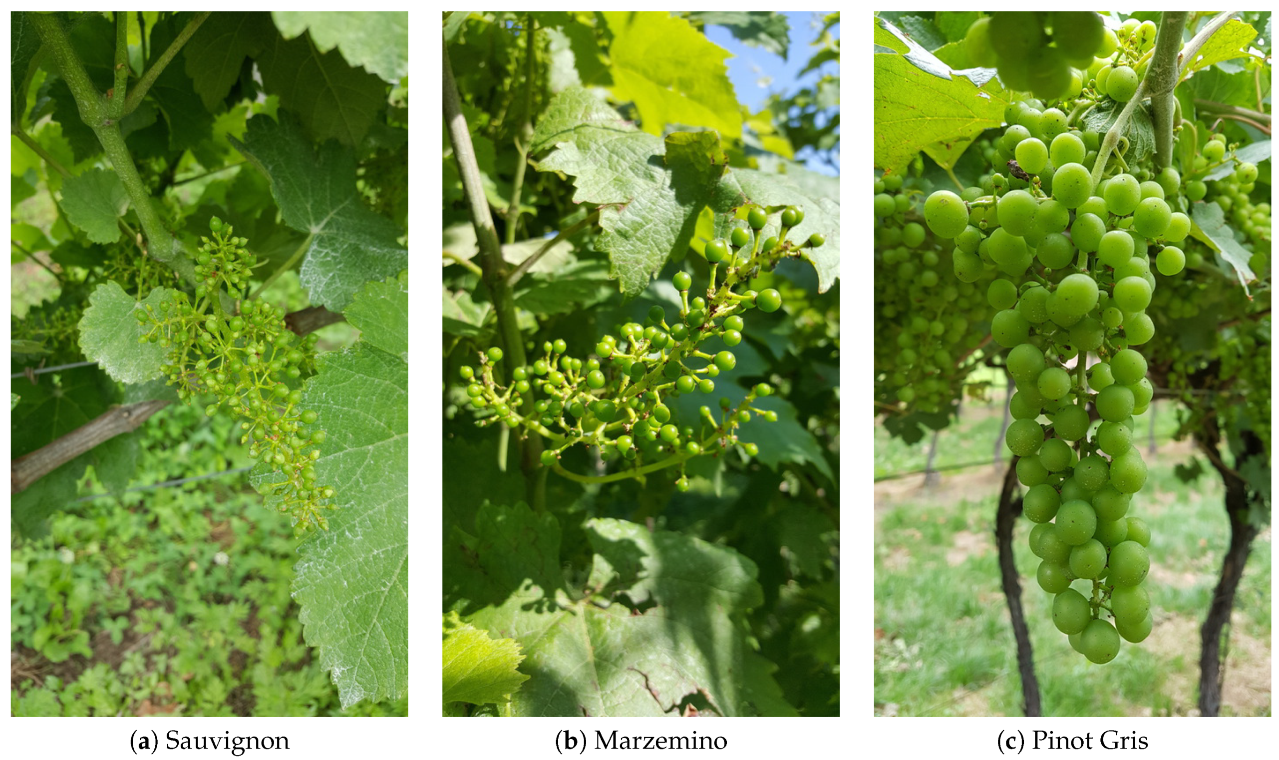
The CR1 dataset collects pictures of seven different varieties: the performances of the network for each variety is reported in Table 5 and Table 6. The difference in performance reflects that having collected the pictures in the same days for all the varieties implies a non-uniform phenological state, yielding highly different visual features exemplified in Figure 6. Although this difference among varieties impacts the performances of GBCNet on single image prediction, the model is capable of obtaining a low MAE by aggregating the output predictions for almost all the varieties.
Table 7 collects results for GBCNet tested on CR2 dataset with 3-CV. Considering single images predictions with an average of 1113.9 berries per picture, the model reaches a MAE of 117.36 berries for each validation fold (10.74%). The overall MAE obtained comparing the cumulative sum of predictions and ground truth (6288.3 berries in average for each fold) results in lower value, i.e., 466.53 (7.24%), benefiting from the balancing effect of over- and underestimation when aggregating predictions.
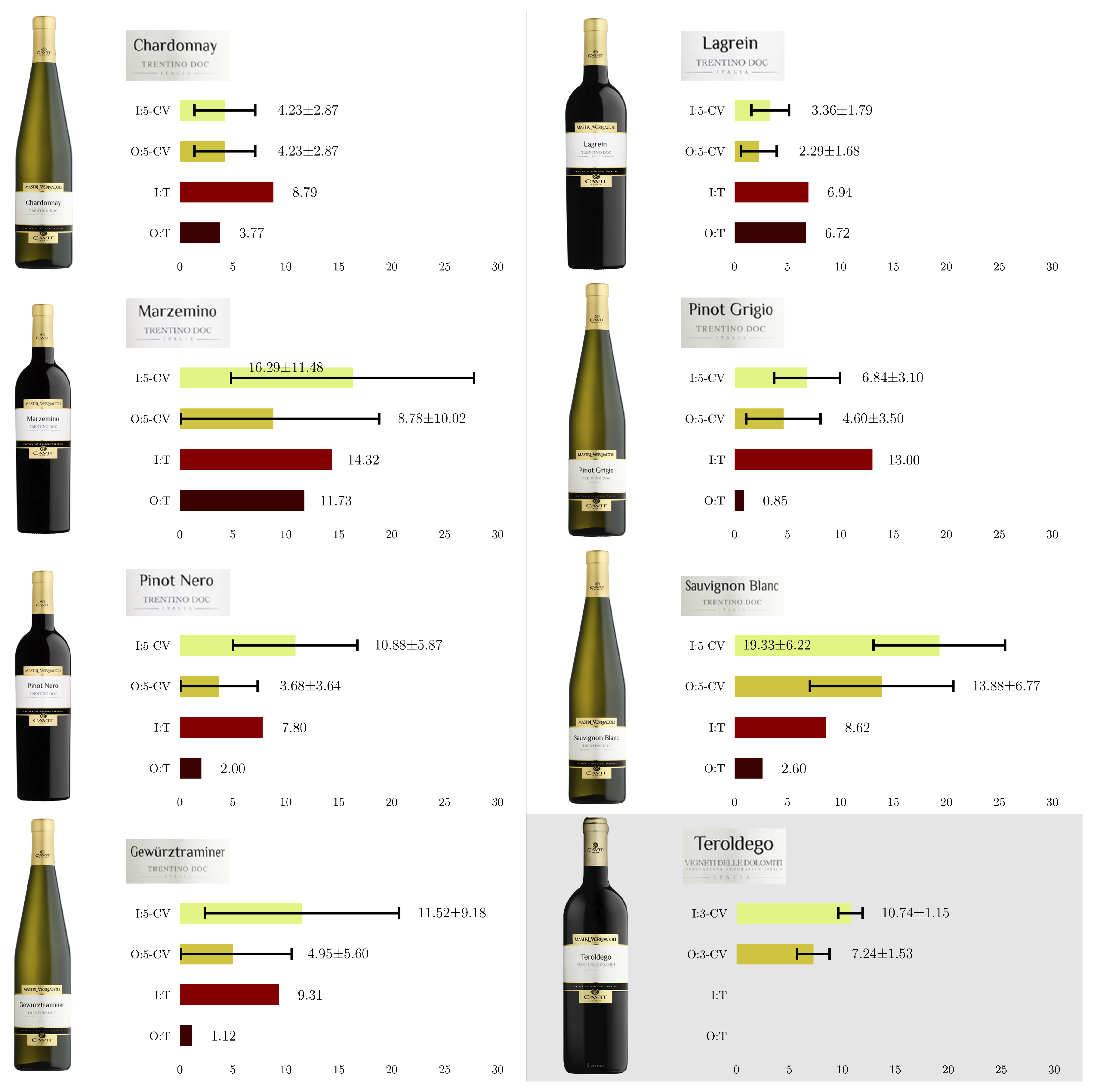
In Figure 7 we graphically report the MAE(%) for all varieties and for all the experimental conditions: these results are fully comparable with what was obtained with the alternative methods available in the literature, but where the images are taken in a controlled environment or employing a capturing box to limit background interference.
As stated in Section 2 (Preliminaries), the estimation of the number of berries is the crucial parameter for having an accurate prediction of the yield. Having proved that the error on counting berries is of the order of a few percentage points, we are allowed to use Equation (2) to arrive at the final goal of estimating the grape production.
5. Conclusions
We demonstrate that crop yield estimation for grape berries can be obtained using smartphone cameras with fixed-focus small aperture wide angle optical systems by the DL architecture GBCNet, an adaptation of algorithms for crowd counting. Although other factors (see Equations (1) and (2)) have to be considered for an actual yield estimate, the average test error of about for the berry counting model is considered valid for operational application (, according to the vine training system). In this study, all data were collected directly in the field and without requiring special cautions or additional constraints, such as a backing board. Notably, the average test error systematically decreases by estimating over more than three pictures from the same parcel. For the Pinot Gris, with a test set of seven images (for a total of about 1300 berries), the percentage MAE is less than .
Further research will investigate, in the same setup, the problem of estimating clusters’ weight, thus considering a correcting factor for non-visible berries.
Author Contributions
Conceptualization, L.C. and M.C.; methodology, L.C. and M.C.; software, L.C.; validation, L.C. and M.C.; formal analysis, M.C.; investigation, L.C. and M.C.; resources, M.C.; data curation, L.C.; writing—original draft preparation, C.F. and G.J.; writing—review and editing, G.J., M.C. and C.F.; visualization, L.C.; supervision, C.F.; project administration, C.F.; funding acquisition, C.F. and G.J. All authors have read and agreed to the published version of the manuscript.
Funding
Research project partially funded by CAVIT s.c., Trento. L. C. is supported by “Orio Carlini” scholarship, GARR Consortium.
Acknowledgments
Authors thank Andrea Faustini and CAVIT s.c. for providing data and scientific support throughout all phases of the research.
Conflicts of Interest
The authors declare no conflict of interest. The funders had no role in the design of the study; in the collection, analyses, or interpretation of data; in the writing of the manuscript, or in the decision to publish the results.
Abbreviations
The following abbreviations are used in this manuscript:
| AI | Artificial Intelligence |
| CNN | Convolutional Neural Network |
| CV | Cross-Validation |
| CSRNet | Congested Scene Recognition Network |
| DL | Deep Learning |
| VGG-16 | Oxford Visual Geometry Group v.16 |
| MAE | Mean Absolute Error |
| MCNN | Multi-scale Convolutional Neural Network |
| MSE | Mean Squared Error |
References
- Schrijver, R. Precision Agriculture and the Future of Farming in Europe; Technical Report Scientific Foresight Study IP/G/STOA/FWC/2013-1/Lot 7/SC5; European Parliament Research Series; Scientific Foresight Unit (STOA): Brussels, Belgium, 2016. [Google Scholar]
- Seng, K.P.; Ang, L.M.; Schmidtke, L.M.; Rogiers, S.Y. Computer Vision and Machine Learning for Viticulture Technology. IEEE Access 2018, 6, 67494–67510. [Google Scholar] [CrossRef]
- Lüttich, F.R. Predictive Models for Smart Vineyards. Master’s Thesis, Stellenbosch University, Stellenbosch, South Africa, 2019. [Google Scholar]
- Food and Agriculture Organization of the United Nations (FAO). The Future of Food and Agriculture. Trends and Challenges; Technical Report; FAO: Rome, Italy, 2017. [Google Scholar]
- Zabawa, L.; Kicherer, A.; Klingbeil, L.; Milioto, A.; Töpfer, R.; Kuhlmann, H.; Roscher, R. Detection of Single Grapevine Berries in Images Using Fully Convolutional Neural Networks. In Proceedings of the 2019 IEEE/CVF Conference on Computer Vision and Pattern Recognition Workshops (CVPRW), Long Beach, CA, USA, 16–21 June 2019; pp. 2571–2579. [Google Scholar]
- Zabawa, L.; Kicherer, A.; Klingbeil, L.; Töpfer, R.; Kuhlmann, H.; Roscher, R. Counting of grapevine berries in images via semantic segmentation using convolutional neural networks. ISPRS J. Photogramm. Remote Sens. 2020, 164, 73–83. [Google Scholar] [CrossRef]
- Nellithimaru, A.K.; Kantor, G.A. ROLS: Robust Object-Level SLAM for Grape Counting. In Proceedings of the 2019 IEEE/CVF Conference on Computer Vision and Pattern Recognition Workshops (CVPRW), Long Beach, CA, USA, 16–21 June 2019; pp. 2648–2656. [Google Scholar]
- Millan, B.; Velasco-Forero, S.; Aquino, A.; Tardaguila, J. On-the-Go Grapevine Yield Estimation Using Image Analysis and Boolean Model. J. Sens. 2018, 2018, 9634752. [Google Scholar] [CrossRef]
- Kurtser, P.; Ringdahl, O.; Rotstein, N.; Berenstein, R.; Edan, Y. In-Field Grape Cluster Size Assessment for Vine Yield Estimation Using a Mobile Robot and a Consumer Level RGB-D Camera. IEEE Robot. Autom. Lett. 2020, 5, 2031–2038. [Google Scholar] [CrossRef]
- Hacking, C.; Poona, N.; Manzan, N.; Poblete-Echeverría, C. Investigating 2-D and 3-D Proximal Remote Sensing Techniques for Vineyard Yield Estimation. Sensors 2019, 19, 3652. [Google Scholar] [CrossRef] [PubMed] [Green Version]
- Aquino, A.; Millan, B.; Gaston, D.; Diago, M.P.; Tardaguila, J. vitisFlower®: Development and testing of a novel Android-smartphone application for assessing the number of grapevine flowers per inflorescence using artificial vision techniques. Sensors 2015, 15, 21204–21218. [Google Scholar] [CrossRef]
- Di Gennaro, S.F.; Toscano, P.; Cinat, P.; Berton, A.; Matese, A. A Low-Cost and Unsupervised Image Recognition Methodology for Yield Estimation in a Vineyard. Front. Plant Sci. 2019, 10, 559. [Google Scholar] [CrossRef] [Green Version]
- Silver, D.L.; Monga, T. In Vino Veritas: Estimating Vineyard Grape Yield from Images Using Deep Learning. In Proceedings of the 2019 Canadian Conference on Artificial Intelligence: Advances in Artificial Intelligence, Kingston, ON, Canada, 28–31 May 2019; Volume 11489, pp. 212–224. [Google Scholar]
- Liu, S.; Zeng, X.; Whitty, M. 3DBunch: A novel iOS-smartphone application to evaluate the number of grape berries per bunch using image analysis techniques. IEEE Access 2020, 8, 114663–114674. [Google Scholar] [CrossRef]
- Nuske, S.; Achar, S.; Bates, T.; Narasimhan, S.; Singh, S. Yield estimation in vineyards by visual grape detection. In Proceedings of the 2011 IEEE/RSJ International Conference on Intelligent Robots and Systems (IROS), San Francisco, CA, USA, 25–30 September 2011; pp. 2352–2358. [Google Scholar]
- Nuske, S.; Wilshusen, K.; Achar, S.; Yoder, L.; Narasimhan, S.; Singh, S. Automated Visual Yield Estimation in Vineyards. J. Field Robot. 2014, 31, 837–860. [Google Scholar] [CrossRef]
- Liu, S.; Zeng, X.; Whitty, M. A vision-based robust grape berry counting algorithm for fast calibration-free bunch weight estimation in the field. Comput. Electron. Agric. 2020, 173, 105360. [Google Scholar] [CrossRef]
- Pizer, S.M.; Amburn, E.P.; Austin, J.D.; Cromartie, R.; Geselowitz, A.; Greer, T.; ter Haar Romeny, B.; Zimmerman, J.B.; Zuiderveld, K. Adaptive histogram equalization and its variations. Comput. Vision, Graph. Image Process. 1987, 39, 355–368. [Google Scholar] [CrossRef]
- Everingham, M.; Van Gool, L.; Williams, C.K.I.; Winn, J.; Zissermann, A. The Pascal Visual Object Classes (VOC) Challenge. Int. J. Comput. Vis. 2010, 88, 303–338. [Google Scholar] [CrossRef] [Green Version]
- Tabb, A.; Holguín, G.A.; Naegele, R. Using cameras for precise measurement of two-dimensional plant features: CASS. arXiv 2020, arXiv:1904.13187v2. [Google Scholar]
- Pérez-Zavala, R.; Torres-Torriti, M.; Cheein, F.A.; Troni, G. A pattern recognition strategy for visual grape bunch detection in vineyards. Comput. Electron. Agric. 2018, 151, 136–149. [Google Scholar] [CrossRef]
- Di Gennaro, S.F.; Toscano, P.; Cinat, P.; Berton, A.; Matese, A. A precision viticulture UAV-based approach for early yield prediction in vineyard. In Precision Agriculture ’19; Wageningen Academic Publishers: Gelderland, The Netherlands, 2019; pp. 373–379. [Google Scholar]
- Schmidtke, L.M. Developing a Phone-Based Imaging Tool to Inform on Fruit Volume and Potential Optimal Harvest Time; Technical Report CSU 1501; Charles Sturt University for Australian Grape and Wine Authority trading as Wine Australia (Australian Government): Bathurst, Australia, 2018.
- Sa, I.; Ge, Z.; Dayoub, F.; Upcroft, B.; Perez, T.; McCool, C. Deepfruits: A fruit detection system using deep neural networks. Sensors 2016, 16, 1222. [Google Scholar] [CrossRef] [Green Version]
- Keresztes, B.; Abdelghafour, F.; Randriamanga, D.; Da Costa, J.P.; Germain, C. Real-time Fruit Detection Using Deep Neural Networks. In Proceedings of the 14th International Conference on Precision Agriculture (ICPA), Montreal, QC, Canada, 24–27 June 2018; pp. 1–10. [Google Scholar]
- Pereira, C.S.; Morais, R.; Reis, M.J.C.S. Deep Learning Techniques for Grape Plant Species Identification in Natural Images. Sensors 2019, 19, 4850. [Google Scholar] [CrossRef] [PubMed] [Green Version]
- Rahnemoonfar, M.; Sheppard, C. Deep count: Fruit counting based on deep simulated learning. Sensors 2017, 17, 905. [Google Scholar] [CrossRef] [Green Version]
- He, K.; Gkioxari, G.; Dollár, P.; Girshick, R. Mask R-CNN. In Proceedings of the 2017 IEEE International Conference on Computer Vision (ICCV), Venice, Italy, 22–29 October 2017; pp. 2980–2988. [Google Scholar]
- Śkrabánek, P. DeepGrapes: Precise Detection of Grapes in Low-resolution Images. In Proceedings of the 15th IFAC Conference on Programmable Devices and Embedded Systems (PDeS), Ostrava, Czech Republic, 23–25 May 2018; Volume 51, pp. 185–189. [Google Scholar]
- Cecotti, H.; Rivera, A.; Farhadloo, M.; Pedroza, M.A. Grape detection with convolutional neural networks. Expert Syst. Appl. 2020, 159, 113588. [Google Scholar] [CrossRef]
- Santos, T.T.; de Souza, L.L.; dos Santos, A.A.; Avila, S. Grape detection, segmentation, and tracking using deep neural networks and three-dimensional association. Comput. Electron. Agric. 2020, 170, 105247. [Google Scholar] [CrossRef] [Green Version]
- Bresilla, K.; Perulli, G.D.; Boini, A.; Morandi, B.; Corelli Grappadelli, L.; Manfrini, L. Single-Shot Convolution Neural Networks for Real-Time Fruit Detection Within the Tree. Front. Plant Sci. 2019, 10, 611. [Google Scholar] [CrossRef] [Green Version]
- Araya-Alman, M.; Leroux, C.; Acevedo-Opazo, C.; Guillaume, S.; Valdés-Gómez, H.; Verdugo-Vásquez, N.; Pañitrur-De la Fuente, C.; Tisseyre, B. A new localized sampling method to improve grape yield estimation of the current season using yield historical data. Precis. Agric. 2019, 20, 445–459. [Google Scholar] [CrossRef]
- Guerrero-Gómez-Olmedo, R.; Torre-Jiménez, B.; López-Sastre, R.; Maldonado Bascón, S.; Oñoro-Rubio, D. Extremely Overlapping Vehicle Counting. In Proceedings of the 2015 Iberian Conference on Pattern Recognition and Image Analysis (IbPRIA), Santiago de Compostela, Spain, 10–12 June 2015; Volume 9117, pp. 423–431. [Google Scholar]
- Ren, S.; He, K.; Girshick, R.; Sun, J. Faster R-CNN: Towards real-time object detection with region proposal networks. In Proceedings of the Advances in Neural Information Processing Systems 28 (NIPS), Montreal, QC, Canada, 7–12 December 2015; Cortes, C., Lawrence, N.D., Lee, D.D., Sugiyama, M., Garnett, R., Eds.; 2015; pp. 91–99. [Google Scholar]
- Girshick, R. Fast R-CNN Object detection with Caffe. In Proceedings of the 2015 IEEE International Conference on Computer Vision (ICCV), Santiago, Chile, 7–13 December 2015; pp. 1440–1448. [Google Scholar]
- Acuna, D.; Ling, H.; Kar, A.; Fidler, S. Efficient Interactive Annotation of Segmentation Datasets with Polygon-RNN++. In Proceedings of the 2018 IEEE Conference on Computer Vision and Pattern Recognition (CVPR), Salt Lake City, UT, USA, 18–23 June 2018; pp. 859–868. [Google Scholar]
- Xie, W.; Noble, J.A.; Zisserman, A. Microscopy cell counting and detection with fully convolutional regression networks. Comput. Methods Biomech. Biomed. Eng. Imaging Vis. 2018, 6, 283–292. [Google Scholar] [CrossRef]
- Zhang, C.; Li, H.; Wang, X.; Yang, X. Cross-scene crowd counting via deep convolutional neural networks. In Proceedings of the 2015 IEEE Conference on Computer Vision and Pattern Recognition (CVPR), Boston, MA, USA, 7–12 June 2015; pp. 833–841. [Google Scholar]
- Poni, S.; Casalini, L.; Bernizzoni, F.; Civardi, S.; Intrieri, C. Effects of early defoliation on shoot photosynthesis, yield components, and grape composition. Am. J. Enol. Vitic. 2006, 57, 397–407. [Google Scholar]
- Liu, S.; Whitty, M.; Cossell, S. A Lightweight Method for Grape Berry Counting based on Automated 3D Bunch Reconstruction from a Single Image. In Proceedings of the 2015 IEEE International Conference on Robotics and Automation (ICRA), Seattle, WA, USA, 26–30 May 2015. [Google Scholar]
- Font, D.; Tresanchez, M.; Martínez, D.; Moreno, J.; Clotet, E.; Palacín, J. Vineyard Yield Estimation Based on the Analysis of High Resolution Images Obtained with Artificial Illumination at Night. Sensors 2015, 15, 8284–8301. [Google Scholar] [CrossRef] [PubMed] [Green Version]
- Aquino, A.; Barrio, I.; Diago, M.P.; Millan, B.; Tardaguila, J. vitisBerry: An Android-smartphone application to early evaluate the number of grapevine berries by means of image analysis. Comput. Electron. Agric. 2018, 148, 19–28. [Google Scholar] [CrossRef]
- Li, Y.; Zhang, X.; Chen, D. CSRNet: Dilated convolutional neural networks for understanding the highly congested scenes. In Proceedings of the 2018 IEEE Conference on Computer Vision and Pattern Recognition (CVPR), Salt Lake City, UT, USA, 18–23 June 2018; pp. 1091–1100. [Google Scholar]
- Zhang, Y.; Zhou, D.; Chen, S.; Gao, S.; Ma, Y. Single-Image Crowd Counting Via Multi-Column Convolutional Neural Network. In Proceedings of the 2016 IEEE Conference on Computer Vision and Pattern Recognition (CVPR), Las Vegas, NV, USA, 27–30 June 2016; pp. 589–597. [Google Scholar]
- Heinrich, K.; Roth, A.; Breithaupt, L.; Möller, B.; Maresch, J. Yield Prognosis for the Agrarian Management of Vineyards using Deep Learning for Object Counting. In Proceedings of the 14th International Conference on Wirtschaftsinformatik (WI), Siegen, Germany, 24–27 February 2019; pp. 407–421. [Google Scholar]
- Simonyan, K.; Zisserman, A. Very deep convolutional networks for large-scale image recognition. In Proceedings of the 2015 International Conference on Learning Representations (ICLR), San Diego, CA, USA, 7–9 May 2015; pp. 1–14. [Google Scholar]
- Deng, J.; Dong, W.; Socher, R.; Li, L.J.; Li, K.; Li, F.-F. Imagenet: A large-scale hierarchical image database. In Proceedings of the 2009 IEEE Conference on Computer Vision and Pattern Recognition (CVPR), Miami, FL, USA, 20–25 June 2009; pp. 248–255. [Google Scholar]
- Dumoulin, V.; Visin, F. A guide to convolution arithmetic for deep learning. arXiv 2016, arXiv:1603.07285. [Google Scholar]
- Long, J.; Shelhamer, E.; Darrell, T. Fully convolutional networks for semantic segmentation. In Proceedings of the 2015 IEEE Conference on Computer Vision and Pattern Recognition (CVPR), Boston, MA, USA, 7–12 June 2015; pp. 3431–3440. [Google Scholar]
- Lempitsky, V.; Zisserman, A. Learning to count objects in images. In Proceedings of the Advances in Neural Information Processing Systems 23 (NIPS), Vancouver, BC, Canada, 6–9 December 2010; Lafferty, J.D., Williams, C.K.I., Shawe-Taylor, J., Zemel, R.S., Culotta, A., Eds.; 2010; pp. 1324–1332. [Google Scholar]
- Van der Walt, S.; Schönberger, J.L.; Nunez-Iglesias, J.; Boulogne, F.; Warner, J.D.; Yager, N.; Gouillart, E.; Yu, T. scikit-image: Image processing in Python. PeerJ 2014, 2, e453. [Google Scholar] [CrossRef]
- Paszke, A.; Gross, S.; Chintala, S.; Chanan, G.; Yang, E.; DeVito, Z.; Lin, Z.; Desmaison, A.; Antiga, L.; Lerer, A. Automatic differentiation in PyTorch. In Proceedings of the 31st Conference on Neural Information Processing Systems (NIPS 2017), Long Beach, CA, USA, 4–9 December 2017; Wiltschko, A., van Merriënboer, B., Lamblin, P., Eds.; 2017; pp. 1–4. [Google Scholar]
- Sloth Development Team. Sloth. 2017. Available online: https://github.com/cvhciKIT/sloth (accessed on 11 July 2020).
- Kingma, D.P.; Ba, J. Adam: A method for stochastic optimization. In Proceedings of the 2015 International Conference on Learning Representations (ICLR), San Diego, CA, USA, 7–9 May 2015; pp. 1–15. [Google Scholar]
Figure 1.
GBCNet architecture: the model takes in-field smartphone images as the input and estimates a density map in which the integral represents berries count. The second block uses a dilation factor of 2. Every convolutional layer is followed by a ReLU operation, except for the last one.
Figure 1.
GBCNet architecture: the model takes in-field smartphone images as the input and estimates a density map in which the integral represents berries count. The second block uses a dilation factor of 2. Every convolutional layer is followed by a ReLU operation, except for the last one.

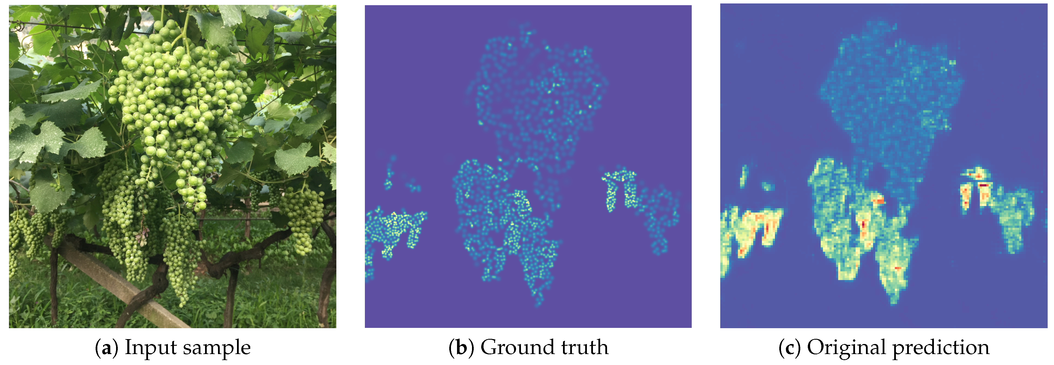
Figure 2.
Example of application of CSRNet on a CR2 image (a), its associated ground truth (b) and model output (c).
Figure 2.
Example of application of CSRNet on a CR2 image (a), its associated ground truth (b) and model output (c).

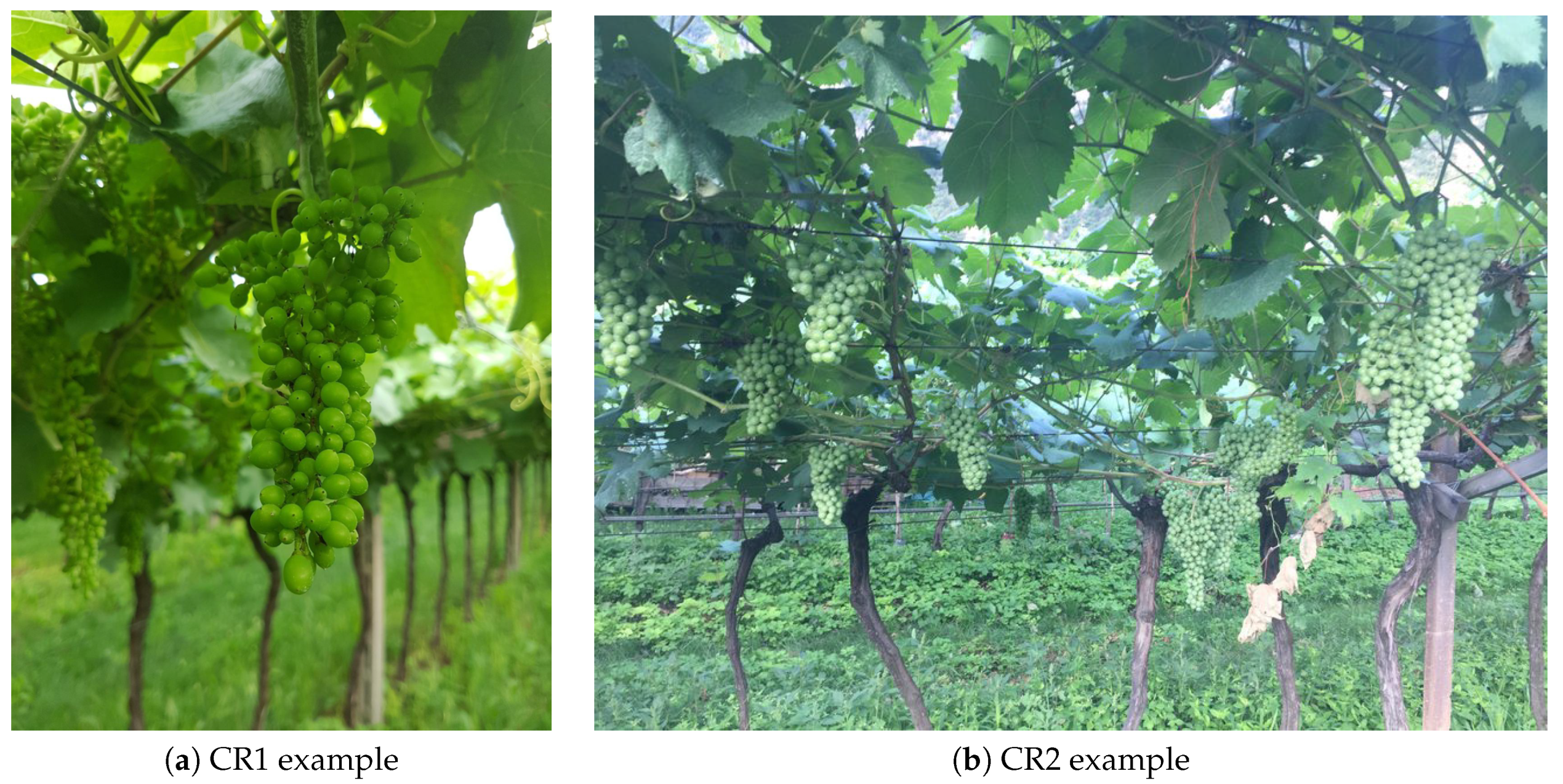
Figure 3.
Example of close-up and medium distance images present in CR1 (a) and CR2 (b) datasets respectively.
Figure 3.
Example of close-up and medium distance images present in CR1 (a) and CR2 (b) datasets respectively.

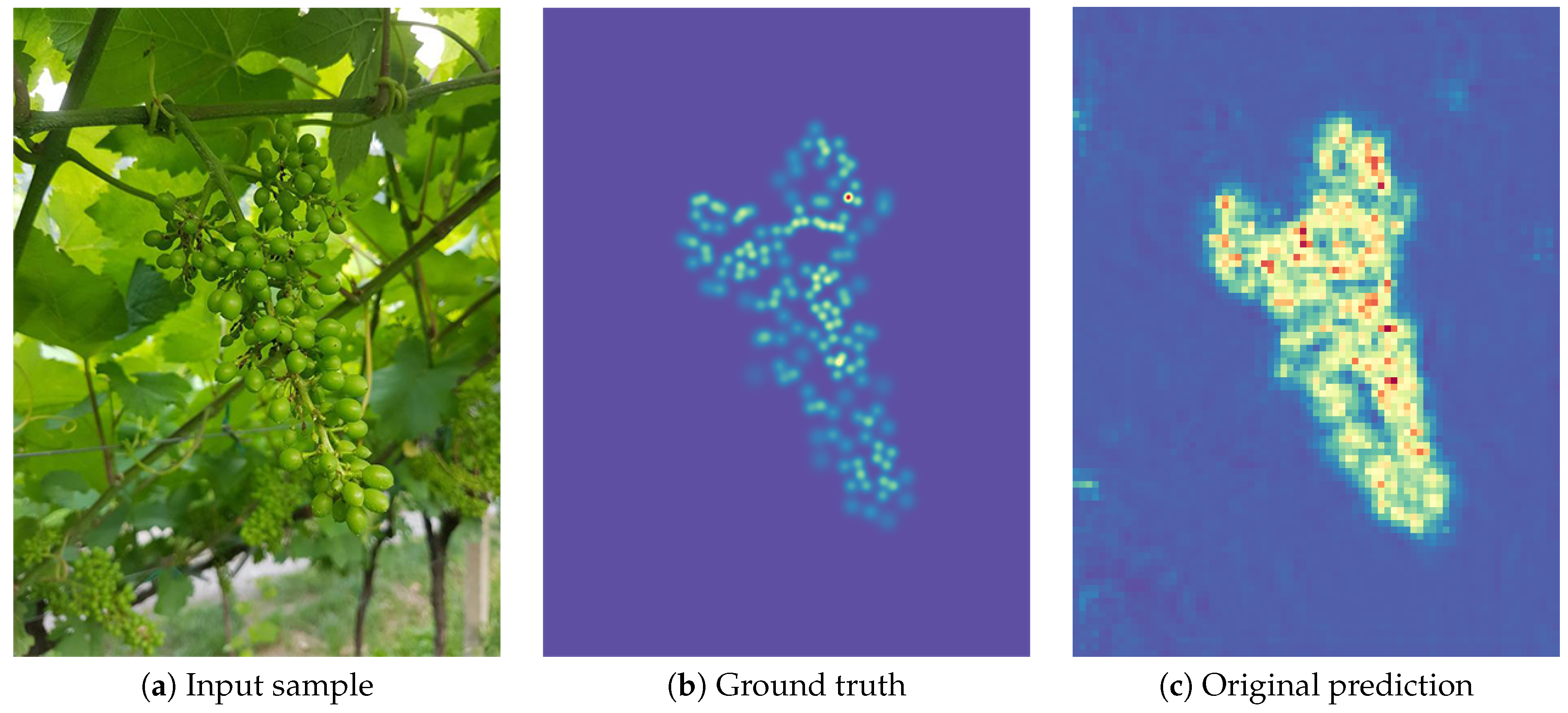
Figure 4.
Example of application of GBCNet on a CR1 image (a), its associated ground truth (b) and model output (c).
Figure 4.
Example of application of GBCNet on a CR1 image (a), its associated ground truth (b) and model output (c).

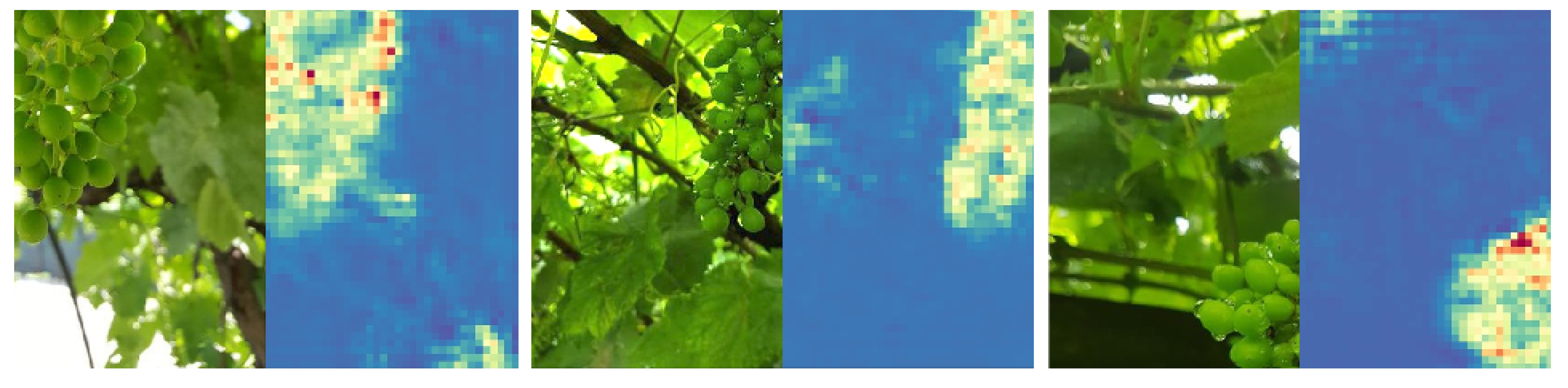
Figure 5.
Examples of CR1 background regions incorrectly highlighted as berry by GBCNet. Overestimation errors are usually associated to patterns with a high variability in brightness and contrast.
Figure 5.
Examples of CR1 background regions incorrectly highlighted as berry by GBCNet. Overestimation errors are usually associated to patterns with a high variability in brightness and contrast.

Figure 6.
CR1 images are collected during the same time period but with different phenological stages depending on the variety. Pictures are sorted by development stage, from less (a) to intermediately (b) to most (c) developed from left to right.
Figure 6.
CR1 images are collected during the same time period but with different phenological stages depending on the variety. Pictures are sorted by development stage, from less (a) to intermediately (b) to most (c) developed from left to right.

Figure 7.
Mean Average Error (MAE) (%) achieved by GBCNet in both cross validation (CV) (5 for CR1 3 for CR2) and test mode by image (I) and overall (O) for all the 8 grape varieties in the two datasets CR1, CR2. All varieties with white background belong to CR1, while Teroldego, in gray background, is CR2. Results are formally reported as mean ± sd, where sd may be larger than mean.


Table 1.
Average cluster weight in grams for different grape varieties in Trentino (Italy) for the five years between 2013 and 2018, with the overall relative deviation V.
Table 1.
Average cluster weight in grams for different grape varieties in Trentino (Italy) for the five years between 2013 and 2018, with the overall relative deviation V.
| 2013 | 2014 | 2015 | 2016 | 2017 | 2018 | V | |
|---|---|---|---|---|---|---|---|
| [g] | [g] | [g] | [g] | [g] | [g] | ||
| Chardonnay | 170 | 184 | 176 | 172 | 172 | 208 | 0.06 |
| Lagrein | 280 | 279 | 325 | 265 | 259 | 264 | 0.06 |
| Marzemino | 308 | 311 | 336 | 326 | 350 | 318 | 0.04 |
| Pinot Gris | 164 | 177 | 181 | 141 | 167 | 205 | 0.09 |
| Pinot Noir | 149 | 174 | 159 | 155 | 158 | 175 | 0.05 |
| Sauvignon Blanc | 169 | 208 | 173 | 163 | 178 | 205 | 0.09 |
| Traminer | 138 | 155 | 174 | 143 | 157 | 151 | 0.06 |
Table 2.
Average single berry weight in grams for different grape varieties in Trentino (Italy) for the years 2016, 2017, 2018, with the overall relative deviation V.
Table 2.
Average single berry weight in grams for different grape varieties in Trentino (Italy) for the years 2016, 2017, 2018, with the overall relative deviation V.
| 2016 | 2017 | 2018 | V | |
|---|---|---|---|---|
| [g] | [g] | [g] | ||
| Chardonnay | 1.6 | 1.6 | 1.7 | 0.03 |
| Lagrein | 1.9 | 2.2 | 2.0 | 0.06 |
| Marzemino | 2.1 | 2.3 | - | 0.05 |
| Pinot Gris | 1.4 | 1.6 | 1.6 | 0.06 |
| Pinot Noir | 1.5 | 1.6 | 1.6 | 0.03 |
| Sauvignon Blanc | - | 1.8 | 1.6 | 0.06 |
| Traminer | 1.4 | 1.7 | 1.7 | 0.08 |
Table 3.
Number of annotated berries per image in the CR1 and CR2 datasets.
| Dataset | Variety | Images | Max | Min | Mean | Total |
|---|---|---|---|---|---|---|
| Chardonnay | 7 | 172 | 51 | 104.71 | 733 | |
| Lagrein | 9 | 211 | 117 | 163.22 | 1469 | |
| Marzemino | 16 | 244 | 53 | 114.81 | 1837 | |
| CR1 | Pinot Gris | 34 | 322 | 86 | 150.91 | 5131 |
| Pinot Noir | 21 | 269 | 93 | 142.00 | 2982 | |
| Sauvignon | 21 | 167 | 42 | 110.38 | 2318 | |
| Traminer | 20 | 207 | 61 | 126.80 | 2536 | |
| Total | 128 | 322 | 42 | 132.90 | 17,006 | |
| CR2 | Teroldego | 17 | 1764 | 535 | 1095.41 | 18,622 |
Table 4.
Application of GBCNet on CR1 5-CV and test sets. The n column refers to the average number of images and berries per fold and in the test set.
Table 4.
Application of GBCNet on CR1 5-CV and test sets. The n column refers to the average number of images and berries per fold and in the test set.
| n | MAE | MAE (%) | MSE | ||
|---|---|---|---|---|---|
| 5-CV | Per Image | 20.4 | 13.66 ± 4.70 | 11.16% ± 2.70% | 18.33 ± 6.33 |
| Overall | 2670.6 | 56.48 ± 60.08 | 2.13% ± 1.97% | ||
| Test | Per Image | 26 | 13.25 | 10.32% | 16.07 |
| Overall | 3653 | 10.65 | 0.29% |
Table 5.
Application of GBCNet on CR1 dataset with 5-CV. Results are reported for all the varieties used in this work, with the average number of images (n) and berries (N) per fold. Results are formally reported as mean ± sd, where sd may be larger than mean.
Table 5.
Application of GBCNet on CR1 dataset with 5-CV. Results are reported for all the varieties used in this work, with the average number of images (n) and berries (N) per fold. Results are formally reported as mean ± sd, where sd may be larger than mean.
| Per Image | Overall | ||||||
|---|---|---|---|---|---|---|---|
| n | MAE | MAE (%) | MSE | N | MAE | MAE (%) | |
| Chardonnay | 1.0 | 4.69 ± 3.53 | 4.23% ± 2.87% | 4.69 ± 3.53 | 112.8 | 4.69 ± 3.53 | 4.23% ± 2.87% |
| Lagrein | 1.4 | 5.41 ± 3.23 | 3.36% ± 1.79% | 5.61 ± 3.51 | 228.2 | 4.63 ± 3.22 | 2.29% ± 1.68% |
| Marzemino | 2.6 | 18.48 ± 17.43 | 16.29% ± 11.48% | 21.29 ± 18.71 | 307.2 | 19.20 ± 16.00 | 8.78% ± 10.02% |
| Pinot Gris | 5.4 | 9.57 ± 3.75 | 6.84% ± 3.10% | 11.59 ± 4.39 | 766.6 | 36.60 ± 27.58 | 4.60% ± 3.50% |
| Pinot Noir | 3.4 | 14.30 ± 8.48 | 10.88% ± 5.87% | 16.08 ± 9.33 | 480.0 | 16.37 ± 13.82 | 3.68% ± 3.64% |
| Sauvignon | 3.4 | 21.35 ± 7.03 | 19.33% ± 6.22% | 25.08 ± 8.51 | 367.0 | 50.55 ± 28.15 | 13.88% ± 6.77% |
| Traminer | 3.2 | 14.02 ± 11.28 | 11.52% ± 9.18% | 15.88 ± 12.72 | 408.8 | 24.02 ± 32.51 | 4.95% ± 5.60% |
Table 6.
Application of GBCNet on CR1 test dataset. Results are reported for each variety, with the number of images (n) and berries (N).
Table 6.
Application of GBCNet on CR1 test dataset. Results are reported for each variety, with the number of images (n) and berries (N).
| Per Image | Overall | ||||||
|---|---|---|---|---|---|---|---|
| n | MAE | MAE (%) | MSE | N | MAE | MAE (%) | |
| Chardonnay | 2 | 7.74 | 8.79% | 8.38 | 169 | 6.38 | 3.77% |
| Lagrein | 2 | 11.03 | 6.94% | 11.88 | 328 | 22.05 | 6.72% |
| Marzemino | 3 | 13.77 | 14.32% | 16.99 | 301 | 35.31 | 11.73% |
| Pinot Gris | 7 | 19.86 | 13.00% | 22.98 | 1298 | 11.08 | 0.85% |
| Pinot Noir | 4 | 10.36 | 7.80% | 10.91 | 582 | 11.62 | 2.00% |
| Sauvignon | 4 | 10.35 | 8.62% | 12.79 | 483 | 12.54 | 2.60% |
| Traminer | 4 | 10.95 | 9.31% | 12.22 | 492 | 5.52 | 1.12% |
Table 7.
Application of GBCNet on CR2 dataset with 3-CV. The n column refers to the average number of images and berries per fold respectively.
Table 7.
Application of GBCNet on CR2 dataset with 3-CV. The n column refers to the average number of images and berries per fold respectively.
| n | MAE | MAE (%) | MSE | |
|---|---|---|---|---|
| Per Image | 5.7 | 117.36 ± 14.07 | 10.74 ± 1.15 | 137.81 ± 18.19 |
| Overall | 6207.3 | 466.53 ± 182.99 | 7.24 ± 1.53 |
© 2020 by the authors. Licensee MDPI, Basel, Switzerland. This article is an open access article distributed under the terms and conditions of the Creative Commons Attribution (CC BY) license (http://creativecommons.org/licenses/by/4.0/).
Share and Cite
MDPI and ACS Style
Coviello, L.; Cristoforetti, M.; Jurman, G.; Furlanello, C. GBCNet: In-Field Grape Berries Counting for Yield Estimation by Dilated CNNs. Appl. Sci. 2020, 10, 4870. https://doi.org/10.3390/app10144870
AMA Style
Coviello L, Cristoforetti M, Jurman G, Furlanello C. GBCNet: In-Field Grape Berries Counting for Yield Estimation by Dilated CNNs. Applied Sciences. 2020; 10(14):4870. https://doi.org/10.3390/app10144870
Chicago/Turabian StyleCoviello, Luca, Marco Cristoforetti, Giuseppe Jurman, and Cesare Furlanello. 2020. "GBCNet: In-Field Grape Berries Counting for Yield Estimation by Dilated CNNs" Applied Sciences 10, no. 14: 4870. https://doi.org/10.3390/app10144870
Note that from the first issue of 2016, this journal uses article numbers instead of page numbers. See further details here.