Aerodynamic Performance of a High-Speed Train Passing through Three Standard Tunnel Junctions under Crosswinds

Abstract

The aerodynamic performance of a high-speed train passing through tunnel junctions under severe crosswind condition was numerically investigated using improved delayed detached-eddy simulations (IDDES). Three ground scenarios connected with entrances and exits of tunnels were considered. In particular a flat ground, an embankment, and a bridge configuration were used. The numerical method was first validated against experimental data, showing good agreement. The results show that the ground scenario has a large effect on the train’s aerodynamic performance. The bridge case resulted in generally smaller drag and lift, as well as a lower pressure coefficient on both the train body and the inner tunnel wall, as compared to the tunnel junctions with flat ground and embankment. Furthermore, the bridge configuration contributed to the smallest pressure variation in time in the tunnel. Overall, the study gives important insights on complicated tunnel junction scenarios coupled with severe flow conditions, that, to the knowledge of the authors, were not studied before. Beside this, the results can be used for further improvements in the design of tunnels where such crosswind conditions may occur.

1. Introduction

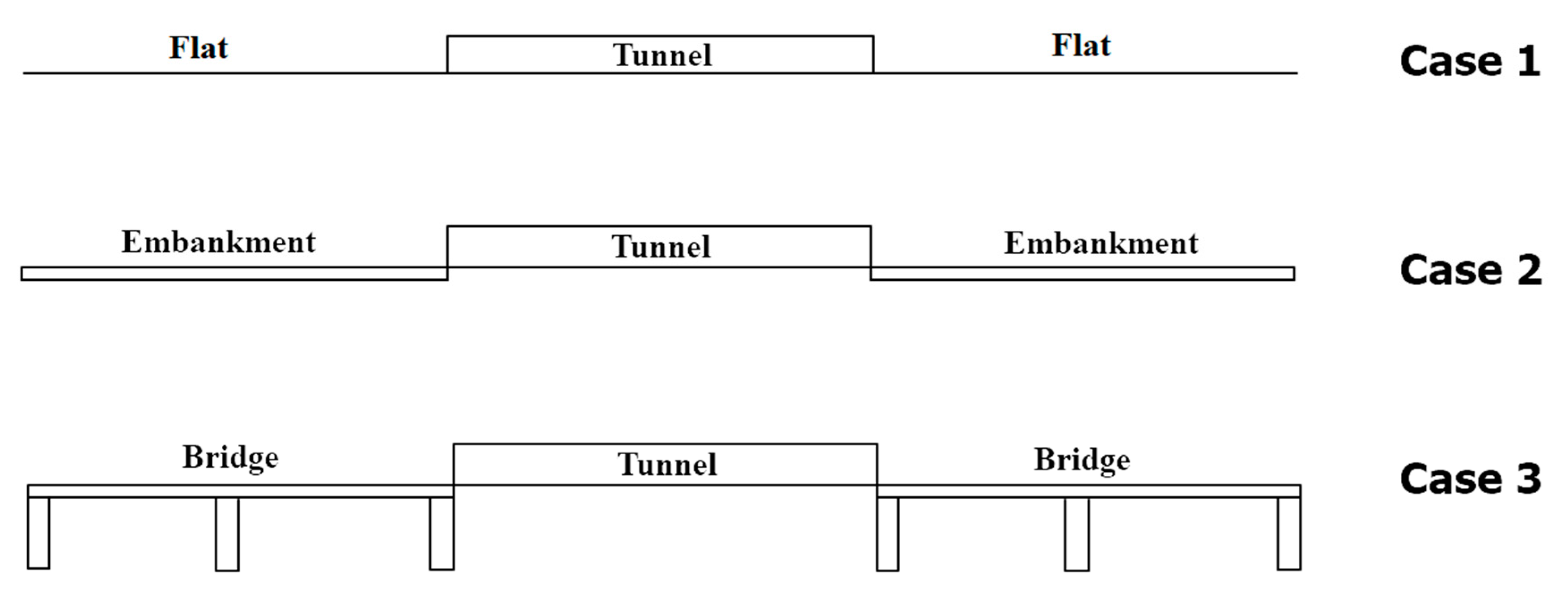
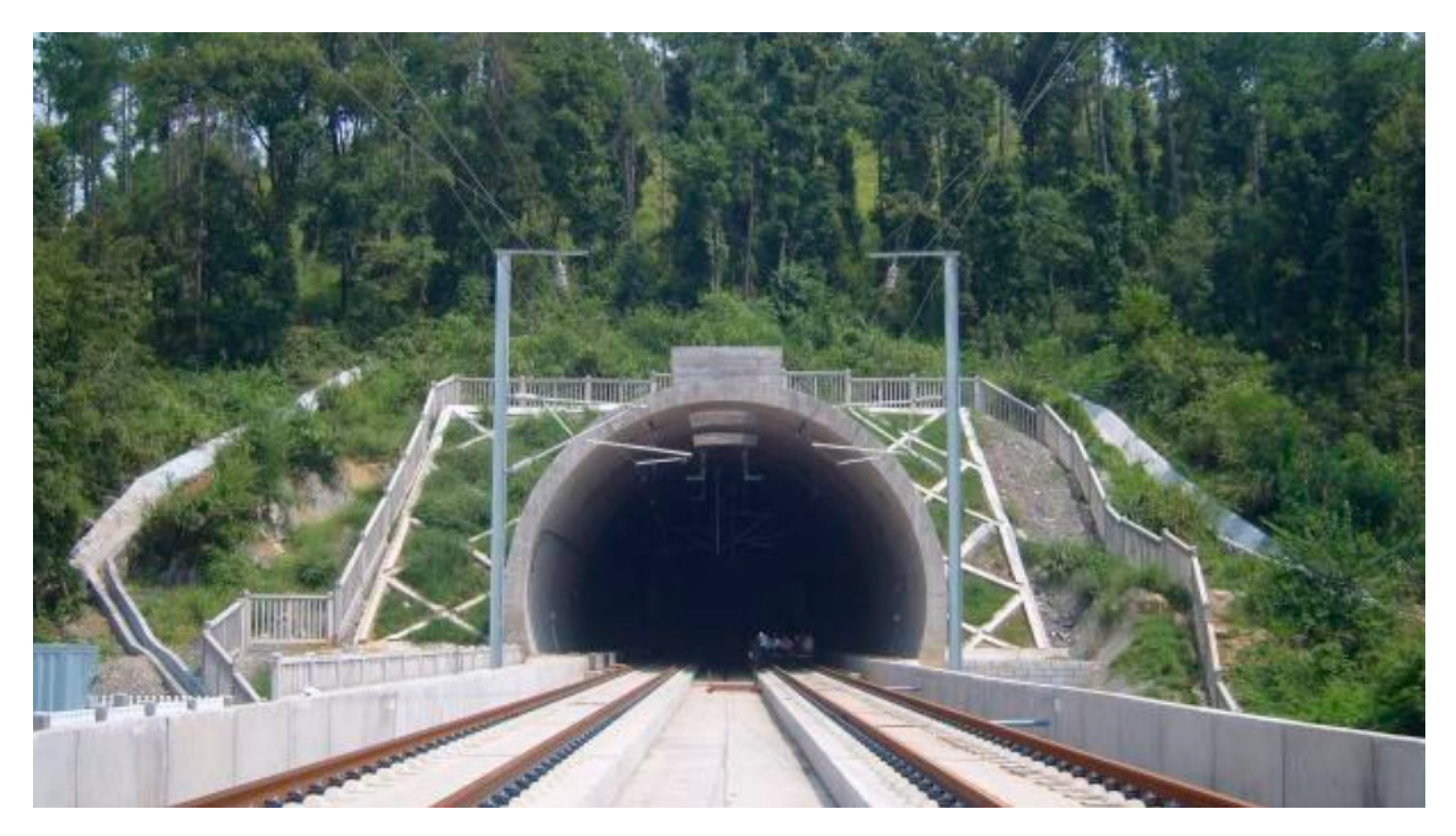
Due to its fast speed, large transportation capacity, and high safety performance, the high-speed train network has been rapidly developed all around the world in the latest decades. However, all these positive aspects come at a price: The train speed significantly impacts its aerodynamic performance, raising problems connected to operational safety and performance. Particularly important is the train’s capability to withstand the effects of strong crosswind, which, in extreme cases, leads to catastrophic events and overturning. The combination of strong and sudden crosswind gusts with high moving speed results in dangerous situations and may increase the risk of derailment. A further aspect to consider is that with the development of technology, high-speed railways have gradually reached mountainous regions. As a result, high-speed railway tunnels have been built to shorten distance between destinations. Subsequently, different junctions, such as flat ground, embankment, and bridge scenarios, are normally found at the entrance and exit of tunnels. For example, the Sichuan-Tibet Railway in China, which is planned to be built in the upcoming years, crosses the Hengduan Mountains and follows the “Seven Mountains and Six Rivers” along its route. High altitude and complex terrain lead to a large number of tunnels along the railways and contributes to significantly different wind conditions as compared to those in plain regions. When the train exits the tunnel, for example, and comes into a strong wind region, the sudden change of the surrounding flow inevitably causes vibrations and poses a direct threat to its safety.

Previous work in this topic has been mostly carried out with experiments using both static and moving models. A static experiment consists of a fixed model and an incoming wind speed. It is generally carried out in wind tunnels in order to evaluate crosswind and Reynolds number effects [1]. In particular, the most prominent studies in the literatures [2,3] have numerically and experimentally shown that crosswind has a strong influence on different aspects of a train’s operational performance and safety. However, several aspects may not be observed with a fixed model in a wind tunnel. For example, with a fixed configuration it is not possible to evaluate the effect of a train moving through a tunnel. To overcome this disadvantage, a moving model configuration can be used. Concerning this method, it has been shown that the flow field around a train will suddenly change because of the relative motion between the train and the surrounding environment which, for example, occur when the train passes through a tunnel [4,5]. Experimental results show that the flow field around a train under a condition of crosswind or passing through a tunnel could be observed by using fixed or moving models, respectively. However, it is still not easy to combine both the investigation of crosswind and tunnel pass-through. Some moving model experiments have been carried out in wind tunnels but restricted by the limited space and moving speed: The Reynolds number was much lower than the actual situation, resulting in a different flow field from the reality [6,7]. For this reason, a methodology which takes into account this aspect should be explored for a deeper analysis.

Numerical simulations are a clearer and reliable solution to overcome the difficult measurements done in experiments. So far, numerical simulations were extensively used to study the flow around fixed trains under crosswind by setting specific inlet flow condition [8,9,10,11,12]. This method is equivalent to the wind tunnel experiment environment, therefore, the train aerodynamic performance in various wind conditions can also be obtained. However, when it is necessary to predict the flow field around a train passing through a tunnel, a moving model need to be considered. On this account, sliding mesh or dynamic mesh techniques were used in many published works [13,14,15,16] successfully simulating moving trains passing through tunnels. Thanks to this, the aerodynamic effect of different railway tunnel conditions observed provided insight for designers of both tunnels and trains. However, there are not many numerical works which have combined the study of side wind with moving trains. It can be found that Krajnović et al. [6] used large eddy simulation (LES) to simulate the flow around a simplified moving train model under crosswind. Their results showed a clear difference in the aerodynamic forces and momentum between the dynamic and static train models. Although a low Reynolds number was used in that case, many valuable pieces of information about the flow field around a moving train under crosswind were provided. Then, Liu [17] numerically studied a train passing by a rectangular windbreak-transition-region, moving from a cutting to an embankment, under crosswind. Their results were compared with full-scale experimental data, showing good agreement. The mentioned studies illustrate that using sliding or dynamic meshes in a crosswind condition is a suitable solution to present this flow condition and can be used to continue doing this work.

The effect of crosswind on a train passing through a tunnel has not been yet fully combined. Only recently, Yang [18] showed that the effect of crosswind locally increases when the train is moving from tunnels into open air as compared to the solely crosswind situation. When a train passes through tunnels, the flow conditions can change suddenly producing a highly complex flow, especially under the condition of crosswind. However, when a train enters and exits a tunnel, it is still unknown how the tunnel junctions affect the train under crosswind. In fact, it can be found that compared to a flat ground, other different subgrades, such as bridges or embankments, have a great influence on the flow around a train [7,19]. Therefore, the coupled effect of different tunnel junctions and crosswind on a moving train needs a thorough understanding. Different scenarios characterize different flow fields, and the present work is an attempt to increase our knowledge about high-speed trains moving through different tunnel junctions under crosswind, identifying the most critical aspects. The conclusion of this present work can provide a starting point for a design reference for the construction of tunnel junctions dedicated to the high-speed railways network.

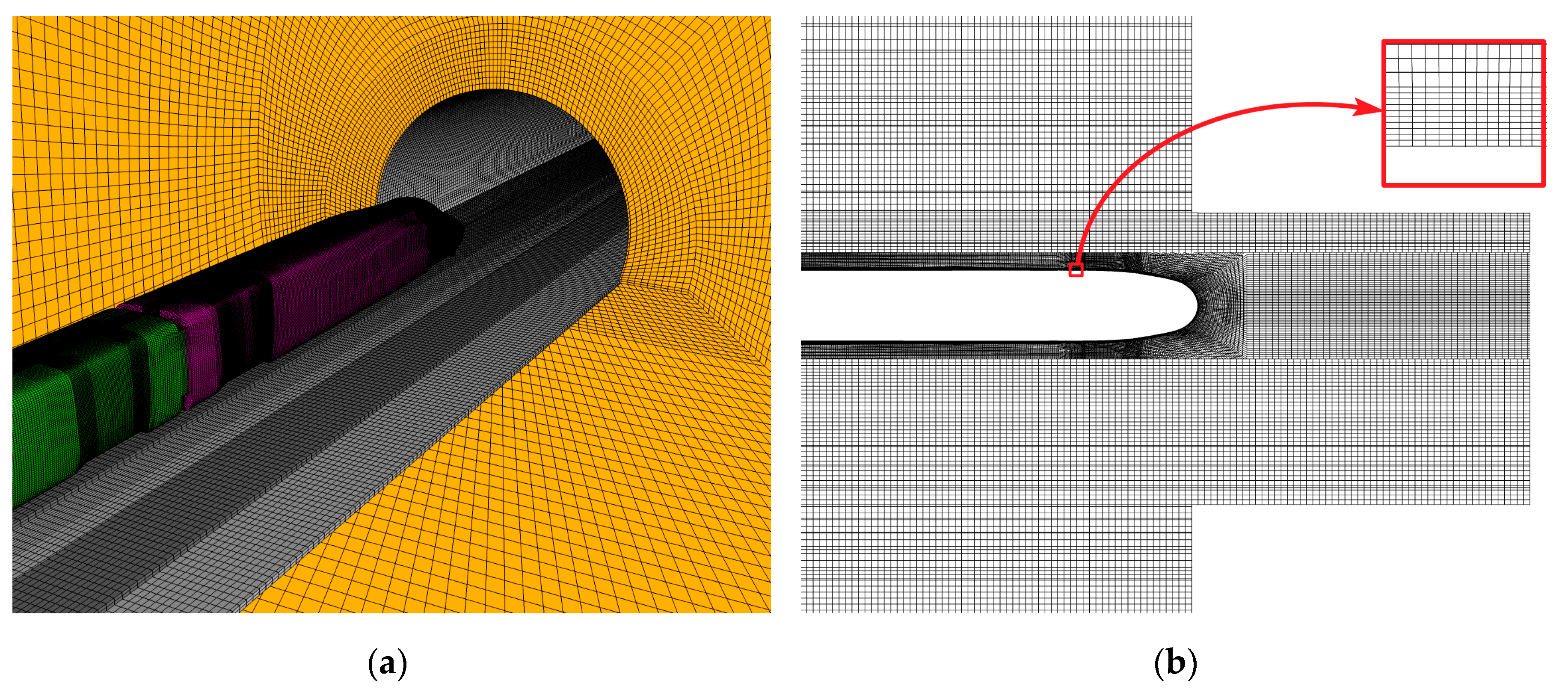
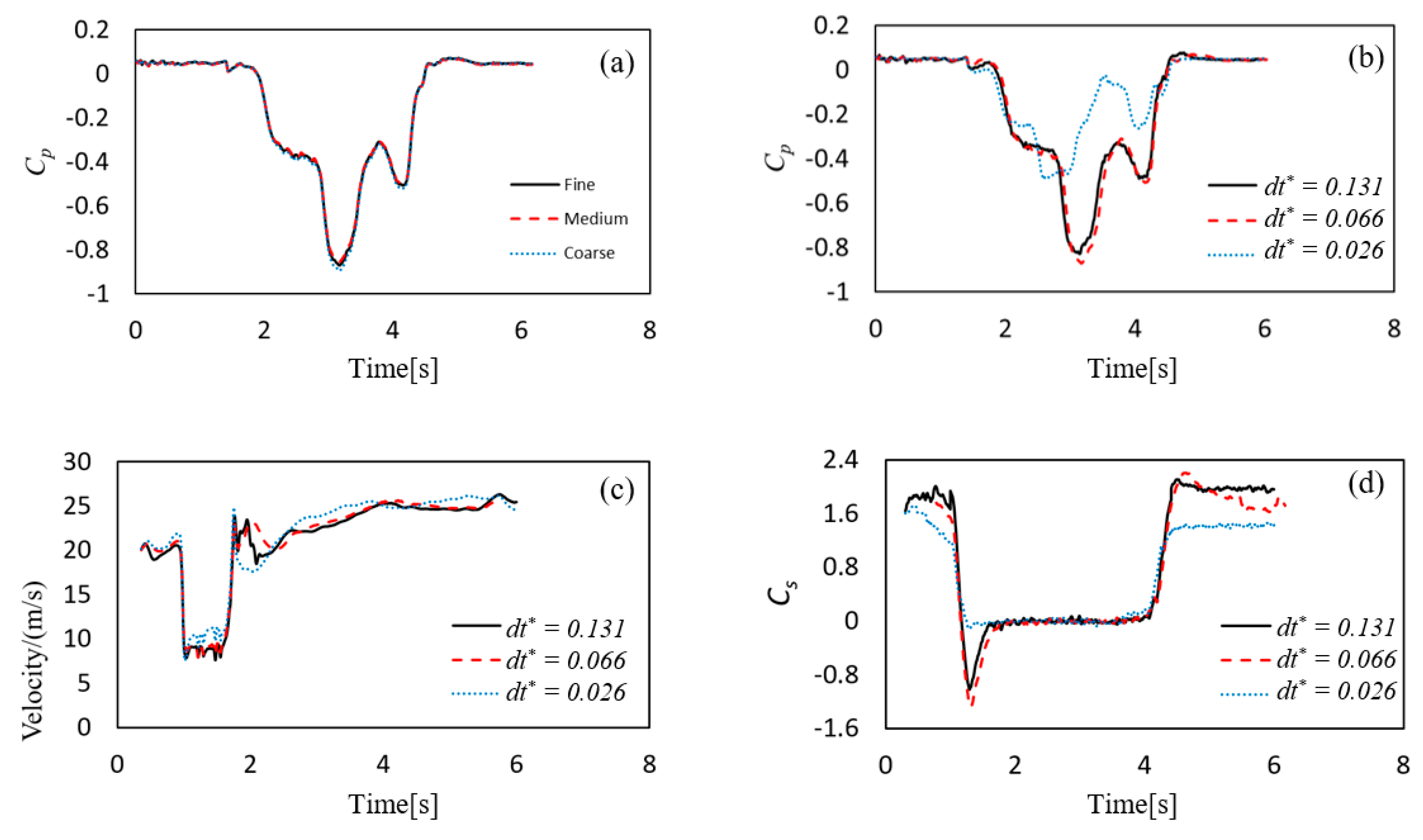
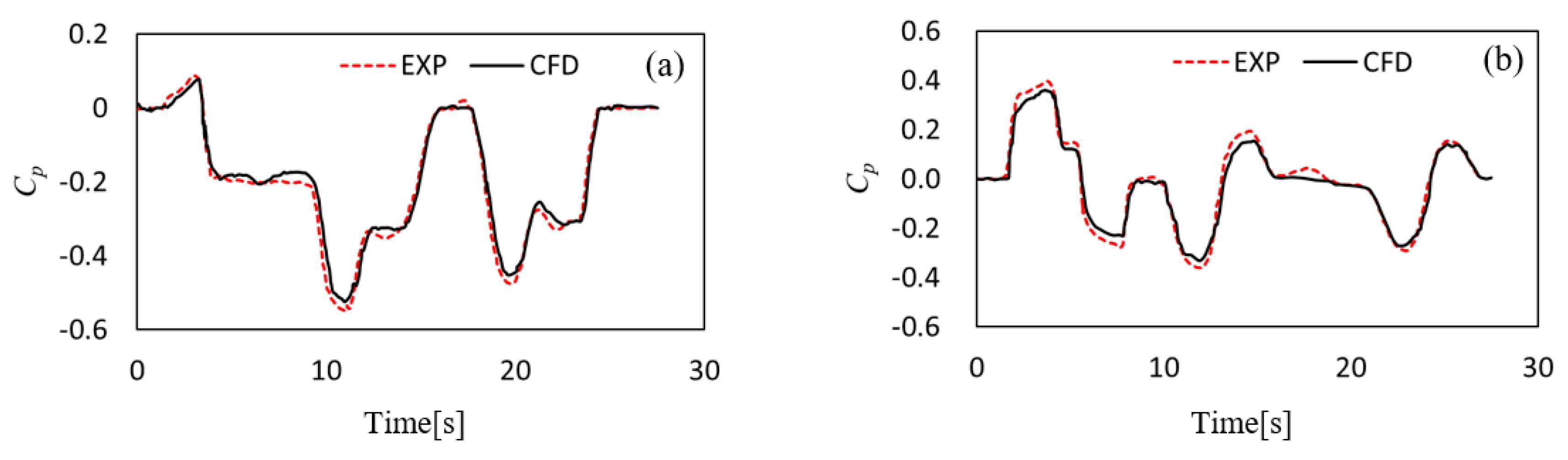
The present paper is organized as follows. In Section 2 the methodology, domain, and mesh generation used for the CFD simulations are given. Grid independence examinations, time step verifications, and a full-scale validation are also reported. In Section 3 the results are discussed focusing on the aerodynamic forces history of high-speed trains passing through tunnel junctions under crosswind. Secondly, the history of pressure on both the train body and the inner tunnel wall is reported. The last part of Section 3 contains a deeper analysis of the pressure distribution, flow streamlines, and flow structures. Conclusions follow in Section 4.

2. Methodology

2.1. Geometry Models

Three kind of junctions are studied in the present work: a flat ground (Case 1), an embankment (Case 2), and a bridge configuration (Case 3), as shown in Figure 2.

The geometry of the model is a simplified CRH2 (China Railway High-speed 2) train, which is composed of a head car (HC), a middle car (MC), and a tail car (TC), as shown in Figure 3a. Figure 3b shows the cross-sections of the embankment, the bridge, and the tunnel used. The models of the CRH2 train, tunnel, embankment, and bridge are not scaled. All the geometry quantities are given in

Table 1. Dimensions of geometric models.

Dimensions of Train	W	L1	L2	L3
/H	0.91	6.95	6.76	6.95
Dimensions of Embankment	WE1	WE2	WE3	WE4	HE
/H	3.62	2.70	0.76	0.59	1.35
Dimensions of Bridge	WB1	WB2	WB3	WB4	HB1	HB2	HB3	HB4	HB5
/H	3.62	1.55	0.76	0.59	0.86	0.81	0.76	0.74	0.65
Dimensions of Tunnel	WT1	WT2	WT3	HT1	HT2
/H	3.57	0.76	0.59	2.32	2.26

, normalized with the height of the train H, which is 3.7 m.

2.2. Numerical Method

The flow around the train is predicted by solving the compressible Navier–Stokes equations together with the energy conservation equation. The commercial finite volume solver ANSYS Fluent 18.0 was used. The improved delayed detached-eddy simulation (IDDES) [20] approach based on the SST k-ω turbulence model [21] was used. The IDDES combines the wall-modelled LES (WMLES) and the delayed detached eddy simulation (DDES) in order to improve the prediction. This method has been applied successfully in previous researches to predict the flow fields for high-speed trains [22,23,24,25,26]. The convective terms and diffusive terms are approximated by an upwind interpolation of second-order accuracy. The time derivative is discretized using the bounded second-order implicit scheme for unsteady flow calculations. The movement of the train is simulated in the present work by sliding meshes, which have been widely used in tunnel aerodynamics for high-speed trains [16,17,27,28]. Figure 4 shows a representative sketch of the main sliding mesh procedure. Nodes a-d on the interface are combined with the nodes A–F on the boundary of the moving domain and nodes G–J on the boundary of the stationary domain surrounding flow. Therefore, the flow information is exchanged between the two domains when simulating the train moving in every time step.

2.3. Numerical Details and Mesh Distributions

The computational domain consists of three parts, i.e., two open-air regions and a tunnel region, as shown in Figure 5. In this work, the CRH2 train moves from the open-air 1 to the open-air 2 through the tunnel at a speed of $v_v$ = 97.22 m·s⁻¹ (approximately 350 km·h⁻¹) under crosswind at a uniform velocity of $v_w$ = 25m·s⁻¹. Both $v_v$ and $v_w$ are constant in time. The Reynolds number based on H is 2.46 × 10⁷. The two open-air regions have an identical size and the dimensions of the domain, normalized with H, are listed in

Table 2. Dimensions of computational domain.

Dimensions	Wo	Lo	Ho	Dl	Dw	HB	LT
/H	81.08	81.08	24.32	27.03	13.51	8.11	81.08

. The top surfaces of the two open-air regions are set as symmetry boundary condition, while the lateral sides closer to the track are treated as mass flow inlets, which means a prescribed mass flow rate is provided. The other two lateral sides are treated as pressure outlets. The two ends are also treated as pressure outlets. All other surfaces are specified as No-slip boundary conditions.

The computational mesh used in the simulation was a structured hexahedral generated using the commercial software Pointwise 18.0. Accuracy was established by simulating the baseline case on three different computational grids which are presented in Section 2.5 in more details. Figure 6 shows some details of the mesh distribution. The mesh near the train is fine enough to capture the turbulent structures near the train model, while those far from the train are relatively coarse. A uniform transition was adopted to generate the mesh. The spatial resolution around the rear part is much finer than that around the rest of the train body. Steady RANS simulations were performed to obtain the initial flow fields. All unsteady simulations were run over t* = t × $v_v$/H = 162. The CFL number was lower than 1 in 99% of the domain. However, there were still some regions near the train body where the CFL number was higher than 1 because of a number of very small cells. A time-step independence study was also performed and reported in Section 2.5. The maximum residual value of the continuity equation to satisfy the convergence criterion was set to 10⁻⁴.

The study conducted by [29] shows that the effect of the Reynolds number on the aerodynamic performance of trains running through tunnels is significant. Therefore, a full-scale model and a realistic Reynolds number in the present study are used. The comparison with experiments shows that the numerical accuracy satisfies the experiments for engineering applications.

2.4. Post-Processing

The aerodynamic forces (the drag, side, and lift forces) and pressure were monitored to investigate the aerodynamic performance of the train when it travels through the three selected junctions under crosswind. The forces and the pressure were normalized to calculate the corresponding coefficients, as follows [30]:

$$C_d=\frac{F_d}{\frac{1}{2}\rho A\left(v_v{}^2+v_w{}^2\right)}$$

(1)

$$C_s=\frac{F_s}{\frac{1}{2}\rho A\left(v_v{}^2+v_w{}^2\right)}$$

(2)

$$C_l=\frac{F_l}{\frac{1}{2}\rho A\left(v_v{}^2+v_w{}^2\right)}$$

(3)

$$C_p=\frac{P-P_{\infty }}{\frac{1}{2}\rho \left(v_v{}^2+v_w{}^2\right)}$$

(4)

$$C_m=\frac{M_o}{\frac{1}{2}\rho AH\left(v_v{}^2+v_w{}^2\right)}$$

(5)

Here, $C_d$, $C_s$, $C_l$, $C_p$, and $C_m$ are the aerodynamic coefficients of drag, side, and lift forces, the pressure and the overturning momentum, respectively. $F_d$, $F_s$, $F_l$, and $P$ are the corresponding forces and pressure. $P_{\infty }$ the reference pressure, $M_o$ is the overturning momentum. $A=11.2$ m² refers to the reference cross-sectional area of the train. $\rho =1.225$ kg·m⁻³ is the air density. $v_v$ and $v_w$ are the velocity of the train and crosswind, respectively.

Two pressure measuring points were virtually mounted on the train body and some on the inner tunnel wall. Figure 7a shows the location of a point on one side of the middle car, and a symmetrical point is found on the other side. Figure 7b shows the location of a point on a cross section of the tunnel wall. Dimensions of the locations of points on the train and on the cross section, normalized with H, are listed in

Table 3. Dimensions of locations of pressure measuring points.

Dimensions	Dp1	Hp1	Dp2	Hp2
/H	3.38	0.46	1.86	0.54
Dimensions	D1	D2	D3	D4	D5	D6	D7	D8	D9
/LT	0.017	0.033	0.067	0.100	0.133	0.167	0.267	0.467	0.500

. The distribution of all 19 cross sections (S₁–₁₉) along the length of the tunnel is shown in Figure 7c. The distances between those points and entrance or exit of the tunnel are normalized with the length of the tunnel, L_T, listed in Table 3. More points are fixed near the entrance and the exit of the tunnel due to expected higher gradients of the flow pressure.

2.5. Grid Independence and Time Step Verification

Previous works [22,23,24,25,26] have shown that grid sizes around 4 × 10⁷ were enough for an IDDES simulation on flow around high-speed trains. However, in order to better verify the accuracy of the results, a grid independence study was performed on three different computational meshes: Fine mesh with 4.6 × 10⁷ elements as described in Section 2.3, medium mesh, containing 4.1 × 10⁷ elements with the cells, and coarse mesh, containing 3.9 × 10⁷ elements. Compared to the fine mesh, the medium and coarse mesh had a lower spanwise and streamwise resolution. The flat ground configuration was used in the grid-independence study. The $C_p$ value at the measurement point located on the windward side of the middle car is shown in Figure 8a. $C_p$ is not sensitive to the mesh resolutions. The maximum difference which occurs at the negative pressure peak is less than 5%, while is generally less than 1%. Thus, the medium mesh was found to be a suitable compromise used to analyze the flow.

The temporal resolution was evaluated by performing simulations on three different time steps, i.e., dt* = t × v_v/H are 0.131, 0.066 and 0.026. $C_p$, velocity magnitude and $C_s$ curves in Figure 8b–d show large differences when the dt* decreases from 0.131 to 0.066. However, a rather small difference is observed between dt* of 0.066 and 0.026. In those comparisons, the monitoring point was located at the track centerline of the tunnel entrance, 0.4 H height above the ground, and $C_s$ was the side force coefficient of the head car. At the two smaller time steps, the difference is less than 1%, except for the negative pressure peak which presents a 5% error. Thus, the dt* = 0.066 is selected as the best compromise between accuracy and computational cost, and later used for the next of the calculations presented in this work.

2.6. Validation

The experimental data from a previously performed full-scale test were used for the validation of numerical accuracy. The real CRH2 train used in the experimental investigation had eight cars, consisting of a head car, six middle cars, and a tail car. The train was moving through the Pingtu tunnel at a speed of 300 km·h⁻¹, Figure 9. The tunnel is 1921 m long and locates on the Beijing–Guangzhou high-speed railway in China. The test system consists of dynamic pressure sensors, multi-core shielded signal lines, a multi-channel amplifier, an A/D converter, a computer, and a GPS speed measurement system. Those pressure sensors have been calibrated before the test so that the measurement error was less than 1%. The length of the tunnel, speed, and the number of cars in the numerical validation is the same as that in the real train experiment.

A comparison of $C_p$ between the experimental and numerical results is shown in Figure 10. In Figure 10a, the monitoring point locates on the outer surface of the fourth train at the middle height. In Figure 10b, the point was 415 m away from the tunnel entrance and 1.5 m above the ground. A good agreement is observed between the experimental and numerical data for the pressure measured on both the train and the wall of the tunnel. The maximum errors of the positive and the negative peak $C_p$ on the train body are around 9% and 5%, respectively, while corresponding quantities observed on the wall of the tunnel are around 9% and 8%. The differences between the numerical results and the experimental data are expected due to the simplifications conducted in the CFD geometry. The physical real-train set-up contains the rail, the side steps, the contact line and other small details that are removed in the numerical model, resulting in a smaller simulation blockage as compared to that in the experiment. This change in the blockage affects the flow field and decreases $C_p$ [31].

3. Analysis and Discussion

In this section, the aerodynamic forces, pressure on the train and inner tunnel wall, flow structures, and velocity field around the train, are analyzed for the sake of showing the aerodynamic performance of the high-speed trains among three cases.

3.1. Aerodynamic Load Coefficients

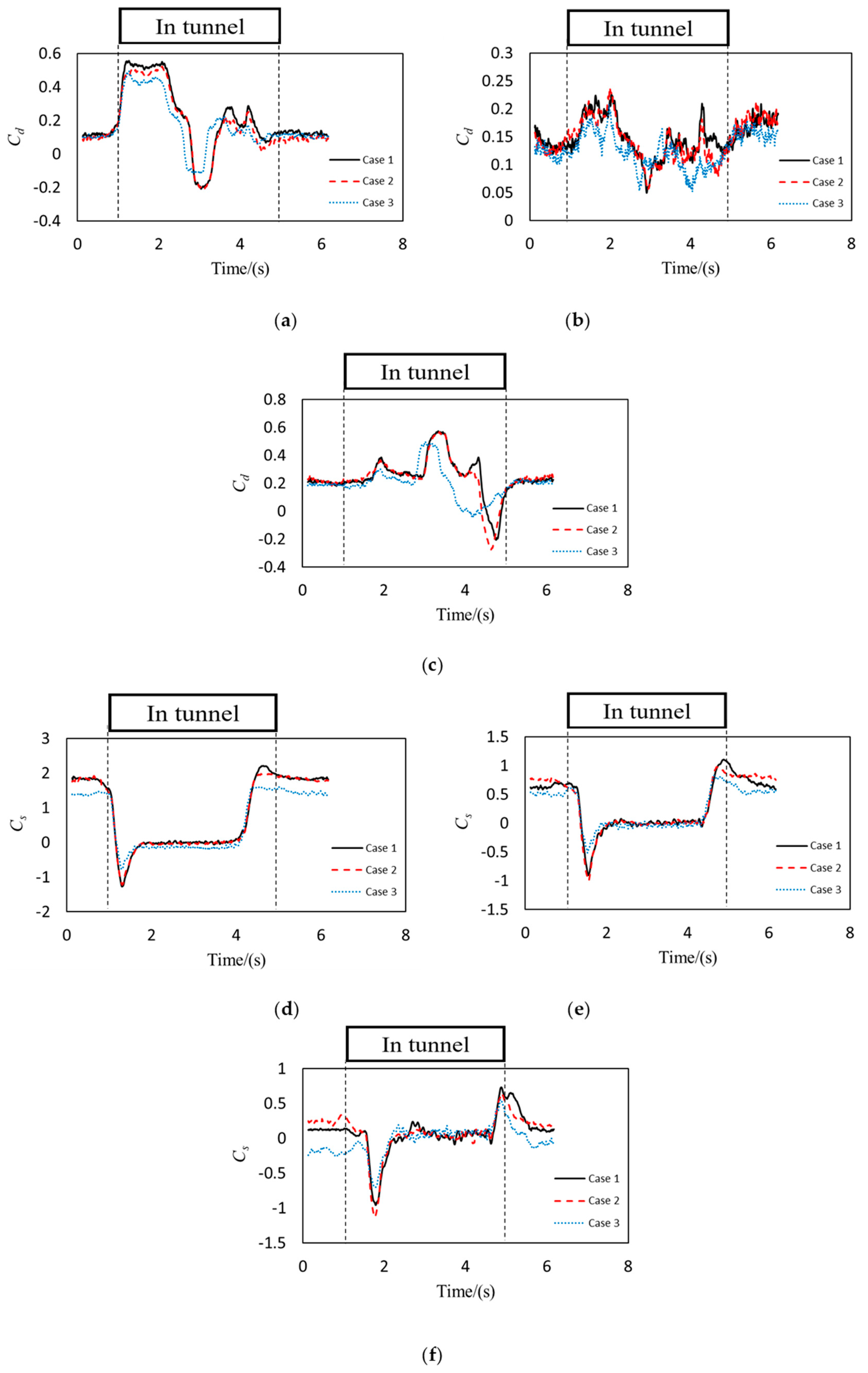
Figure 11 reports the histories of aerodynamic coefficients of three cars in Cases 1–3. The “in tunnel” highlights the period from when head car is entering the tunnel (t = 1.03 s) to the instant the tail car is leaving the tunnel (t = 4.9 s). As to $C_d$, a slight difference is observed when the train is in two open-air regions before or after crossing the tunnel, showing the drag is independent on the ground scenarios. However, when the train passes through the tunnel, Case 3 shows a smaller amplitude compared to Case 1 and Case 2. It is also can be seen that the drag on the head and tail cars is more effected than the middle car. From this, it can be believed that the different ground scenarios outside the tunnel could affect the aerodynamic drag of the train running in the tunnel, and the tunnel junction with the bridge gives a lower drag fluctuation for a running train inside the tunnel.

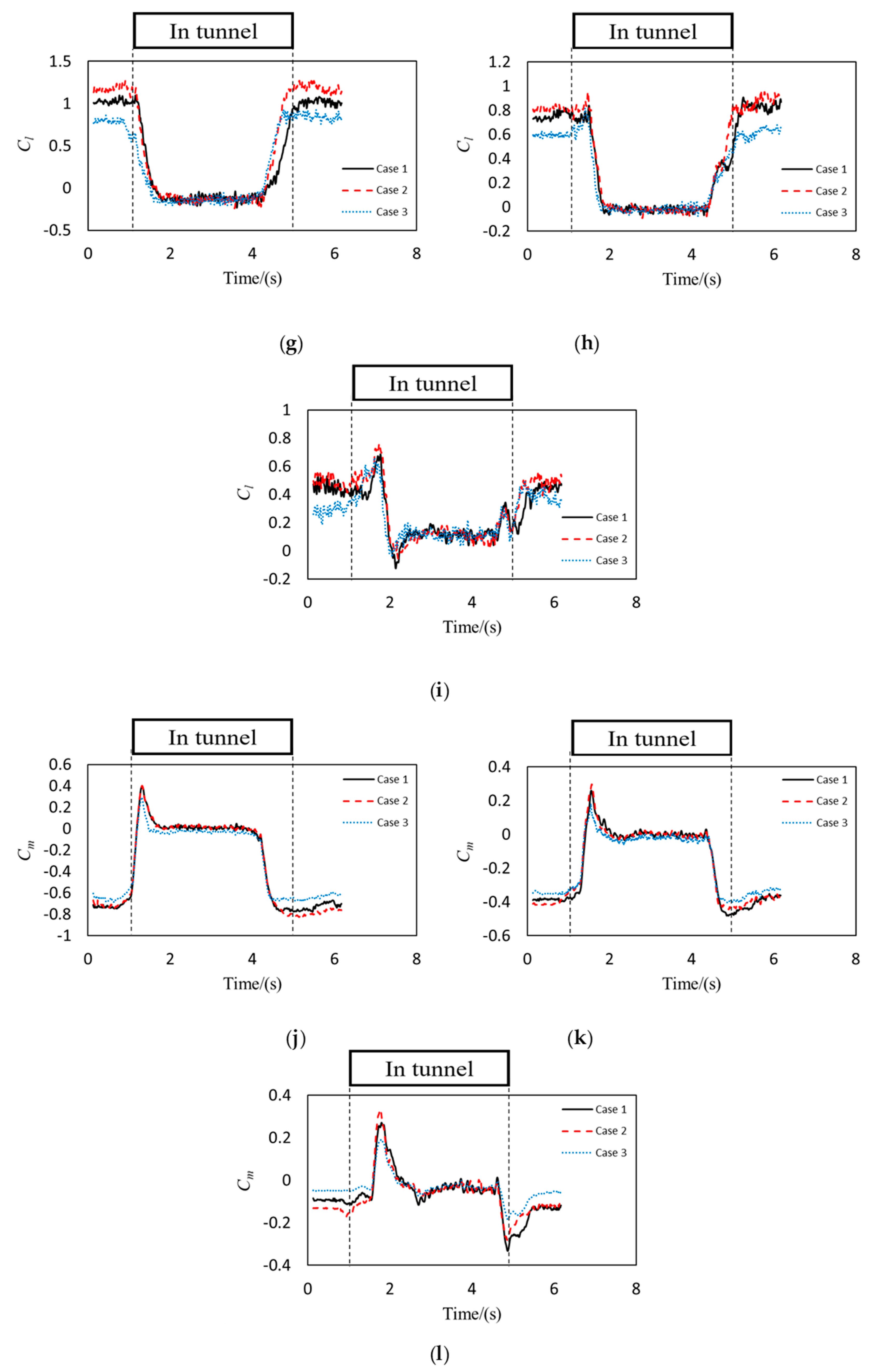
The side ($C_s$) force, lift ($C_s$) force and momentum ($C_m$) show different trends from the drag force coefficient, as shown in Figure 11d–l. The train in Case 3 experiences lower momentum, side and lift forces in the two open-air regions. Then, it can be seen that the momentum, side and lift forces also fluctuate during the period when the train is entering and leaving the tunnel, and the smaller fluctuations are also observed in Case 3, which means the tunnel junction with the bridge also gives lower fluctuations of momentum, side, and lift forces on the train when crossing the tunnel under crosswind.

The peak to peak values of the aerodynamic coefficients are listed in

Table 4. Amplitude values of aerodynamic coefficients.

		Entering the Tunnel			Leaving the Tunnel
		HC	MC	TC	HC	MC	TC
$C_d$	Case 1	0.461	0.105	0.189	0.220	0.096	0.446
	Case 2	0.444	0.100	0.156	0.245	0.105	0.549
	Case 3	0.401	0.085	0.141	0.113	0.074	0.279
$C_s$	Case 1	3.179	1.613	1.199	2.273	1.166	0.823
	Case 2	3.231	1.802	1.428	2.034	1.034	0.720
	Case 3	2.231	1.148	0.893	1.803	0.922	0.705
$C_l$	Case 1	1.253	0.908	0.811	1.311	0.978	0.453
	Case 2	1.418	0.993	0.818	1.513	1.048	0.556
	Case 3	1.073	0.877	0.705	1.143	0.758	0.438
$C_m$	Case 1	1.137	0.657	0.385	0.823	0.513	0.345
	Case 2	1.152	0.714	0.505	0.864	0.471	0.287
	Case 3	0.985	0.536	0.243	0.676	0.410	0.162

. The largest changes of $C_d$ are observed in Case 1. The reason for this can be attributed to the positive $C_d$ peak, which for Case 1 it has the highest value (Figure 11a–c). The largest changes of $C_s$ and $C_l$ are shown at Case 2, Figure 11d–i. The head car is affected more as compared to the middle and tail cars, when the train entering the tunnel. The train exiting the tunnel results in large changes in $C_d$ and $C_l$ values in Case 2, compared to other two cases, shown in Figure 11a–c and g–i. Figure 11c shows that Case 2 causes a strong negative $C_d$ peak at moment when the train leaving the tunnel. The $C_s$ coefficient at the exit of the tunnel was found to change more in Case 1 than in the other two cases, showing that maximum value of $C_s$ in Case 1 is greater than that of two other cases (Figure 11d–f). Similarly, $C_s$, the changes of $C_m$ for the Case 1 and 2 are larger than Case 3 because their higher values of the $C_m$ occurs in both two open-air regions, as shown in Figure 11j–l.

Overall, when the train enters the tunnel, the head car suffers the largest aerodynamic coefficients. When the train leaves the tunnel, except of $C_d$, the head car still experiences the largest aerodynamic coefficients. Furthermore, it is observed that compare the worst case, the tunnel junction with the bridge gives a result that the amplitude of $C_d$, $C_s$, $C_l$, and $C_m$ decrease by 17%, 34%, 18%, and 26%, respectively when the train is entering the tunnel. While the train exits of the tunnel, the amplitude of $C_d$, $C_s$, $C_l$, and $C_m$ reduce approximately 48%, 28%, 25%, and 26%, respectively.

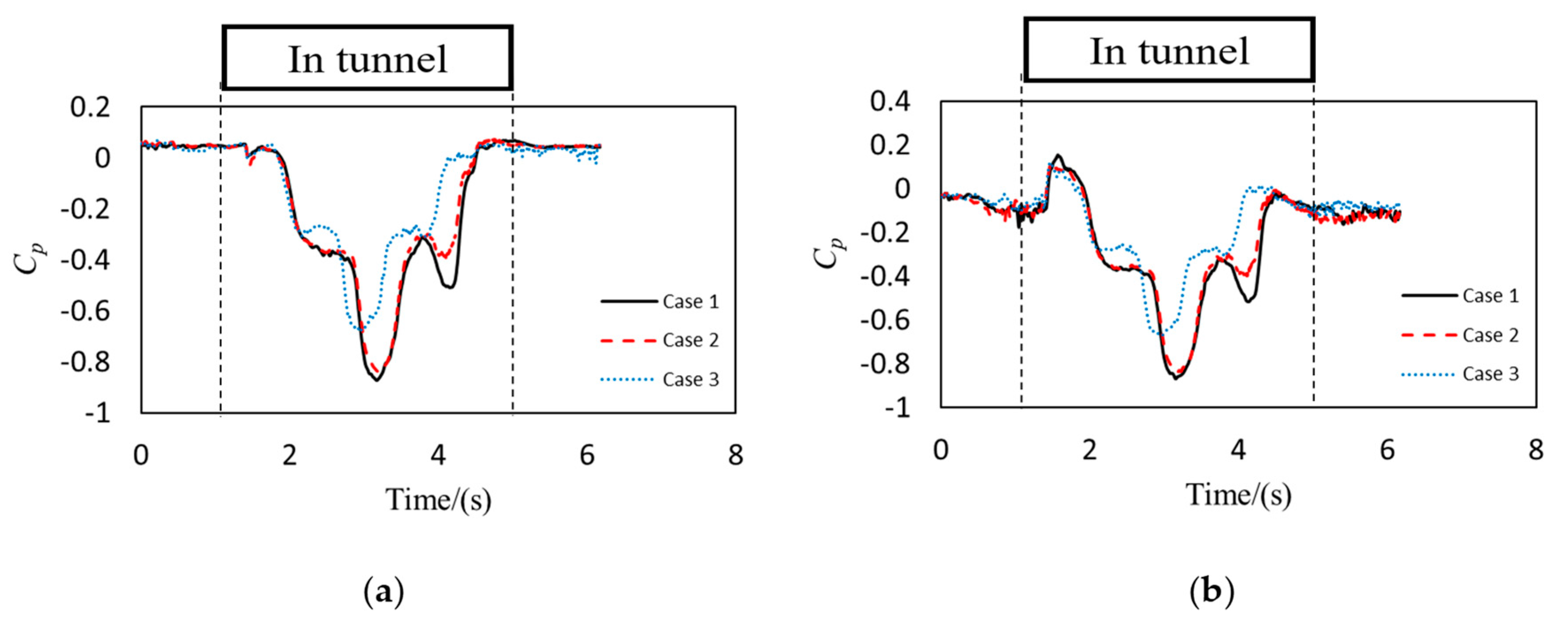
3.2. Pressure Coefficients of the Train

Figure 12 shows the $C_p$ histories at the measuring points on the middle car. $C_p$ is positive on the windward but negative on the leeward side of the train when the train travels under crosswind. The $C_p$ differences in three cases are so small when trains are in the open-air regions. A significant difference of $C_p$ between three cases on both windward and leeward sides of the train, was observed when the train moving through the tunnel. It is interesting to note that Case 3 still shows smaller values of the negative peaks on both sides.

When the train enters the tunnel, $C_p$ on both sides starts to change rapidly, resulting in two negative peaks with large differences in three cases. Figure 12 shows that $C_p$ in Case 2 is slightly smaller at the first peak and much smaller at the secondary peak as compared to Case 1. Then, it can be seen that Case 3 also shows smaller values of the negative peaks on both sides, which means a smaller pressure change on the train surface is provided. It illustrates that the tunnel junction with the bridge gives a better performance of pressure on both sides of the train when crossing a tunnel under crosswind.

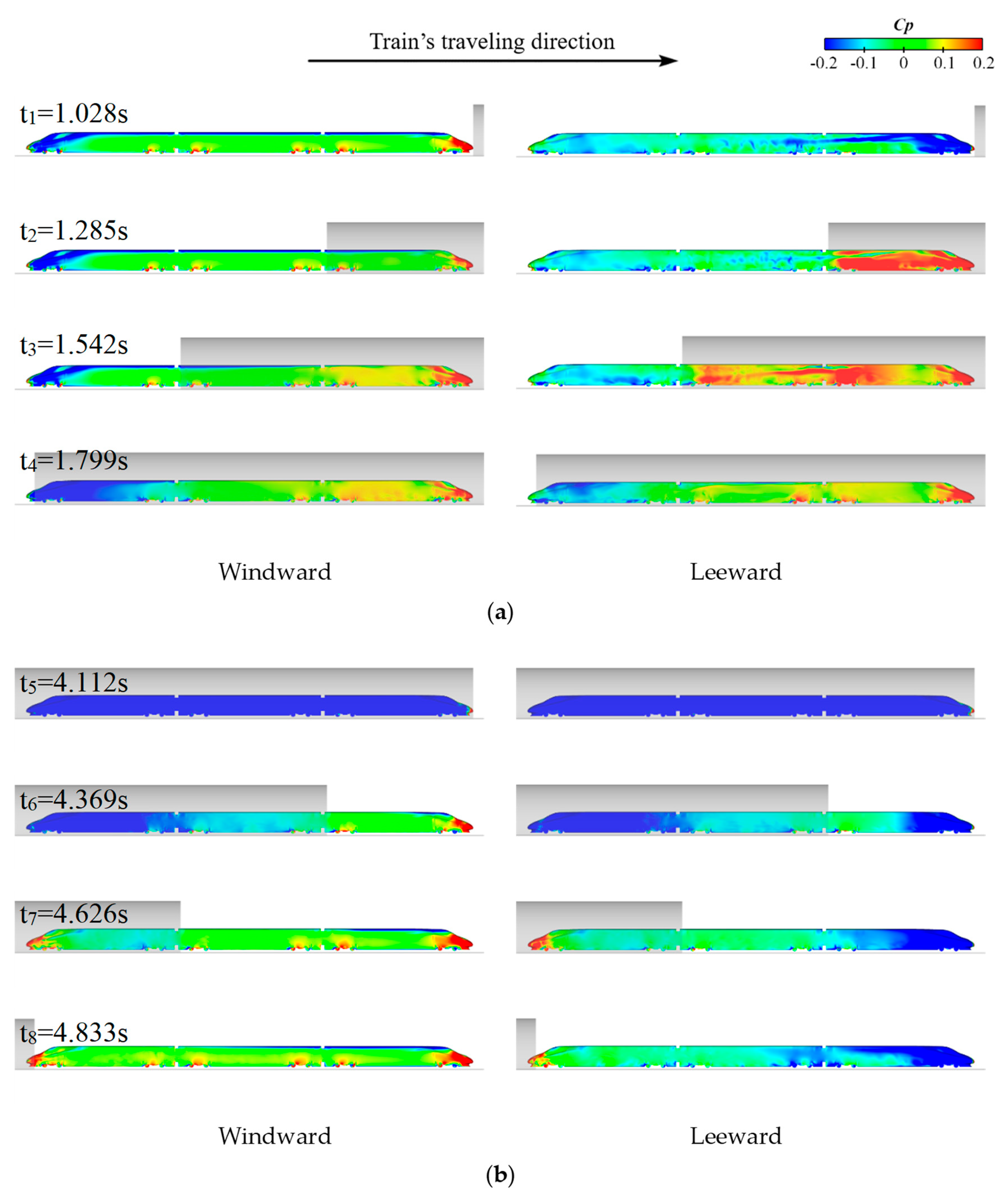
To explore the reason for the largest pressure variation observed in Case 1, an analysis of the surface pressure distribution on both sides of the train is presented in Figure 13 during the process of the train entering (t_1–4) and exiting the tunnel (t_5–8). When the train is entering the tunnel, the surface pressure on the windward side presents a smaller change than that on the leeward side, as shown in Figure 13a. A small difference on the windward side is observed from t₁ to t₂. However, the surface pressure of the head car starts to increase at t₃ and the surface pressure of the tail car begins to decrease at t₄. The change in pressure on the middle car is not significant.

Due to the crosswind, the leeward side of the train experiences negative pressure when the train approaches the entrance of the tunnel at t₁, Figure 13. The surface pressure of the head car suddenly increases and becomes positive as the head car enters the tunnel at t₂. This increase of the pressure continues until the middle car completely enters into the tunnel at t₃. Once the train has entirely entered the tunnel, the surface pressure on the train starts to decrease, as seen in Figure 13a at t₄.

As long as the train stays in the tunnel, no crosswind affects the flow around it, so the surface pressure decreases significantly and becomes negative at time t_5, as shown in Figure 13b. When the train starts to exit the tunnel, the pressure begins increasing with larger change on the windward side of the train (see the period from t₆ to t₈). The surface pressure of each car on the windward side increases and becomes slightly positive when they run into the open-air region. Once the train completely exits the tunnel, the pressure on both sides of the train is generally positive and negative, respectively, due to the effect of the crosswind on the train (see the time at t₈ in Figure 13b).

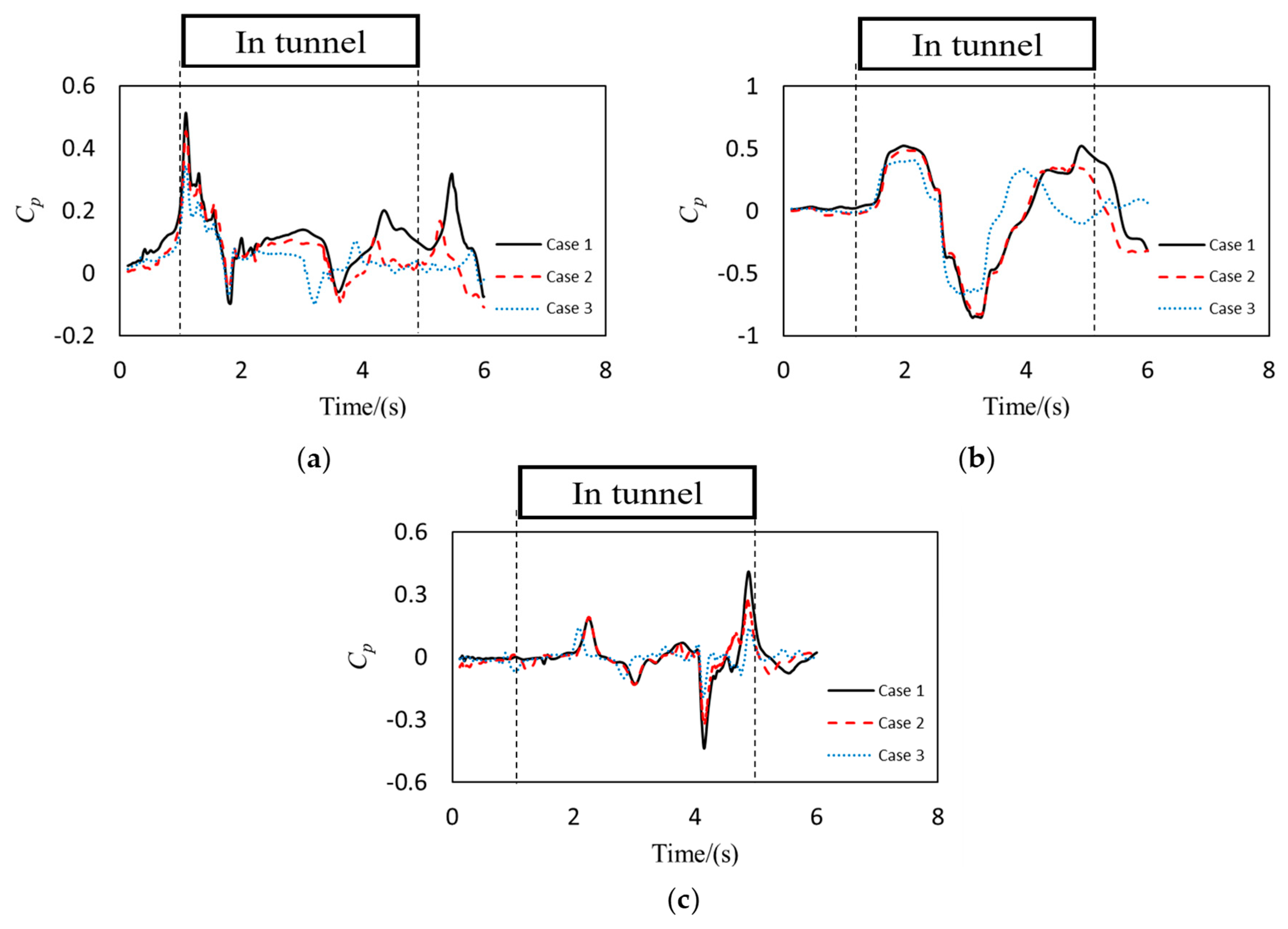
3.3. Pressure Coefficients on the Tunnel Wall

In this section, the pressure fluctuations induced by the train pass-by on the tunnel wall is investigated. Figure 14 shows the $C_p$ histories of several monitoring points along the tunnel wall. At the entrance of the tunnel (S₂), the maximum pressure difference among three cases is found when the train is entering, as shown in Figure 14a. On the other hand, the surface pressure at the exit of the tunnel (S₁₈) shows the maximum difference among cases when the train exits the tunnel, Figure 14c.

Figure 14b shows that the distinct negative $C_p$ peaks are observed in all three cases, when the train moves closer to the middle of the tunnel (S₁₀). As the train is traveling into the tunnel, there is a large change in the surface pressure along the tunnel wall in all three cases. It is interesting to notice that the pressure fluctuation is recorded after the “in tunnel” period, which means that the train-induced wind still affects the flow inside the tunnel for a certain period after the train has left the tunnel. The peaks of pressure in Case 3 show somewhat lower values as compared to the other two cases.

The peak-to-peak values of $C_p$ at different points on the tunnel wall are presented in Figure 15, with the aim to study the variations of maximum pressure along the length of the tunnel in three all cases. All maximum difference values observed in each points at S_1–19 are shown. In general, Case 1 and Case 3 show the largest and smallest peak-to-peak distributions along the tunnel wall, respectively. Therefore, it is confirmed that different ground conditions at junctions have effects on the pressure on the tunnel wall, when the train moves through the tunnel and is subjected to crosswind in the outer regions. The peak-to-peak of pressure in the middle of the tunnel is the largest value in all three cases. Another observation from this figure is that the peak-to-peak values of $C_p$ reduce sharply as the points approach the entrance and the exit of the tunnel.

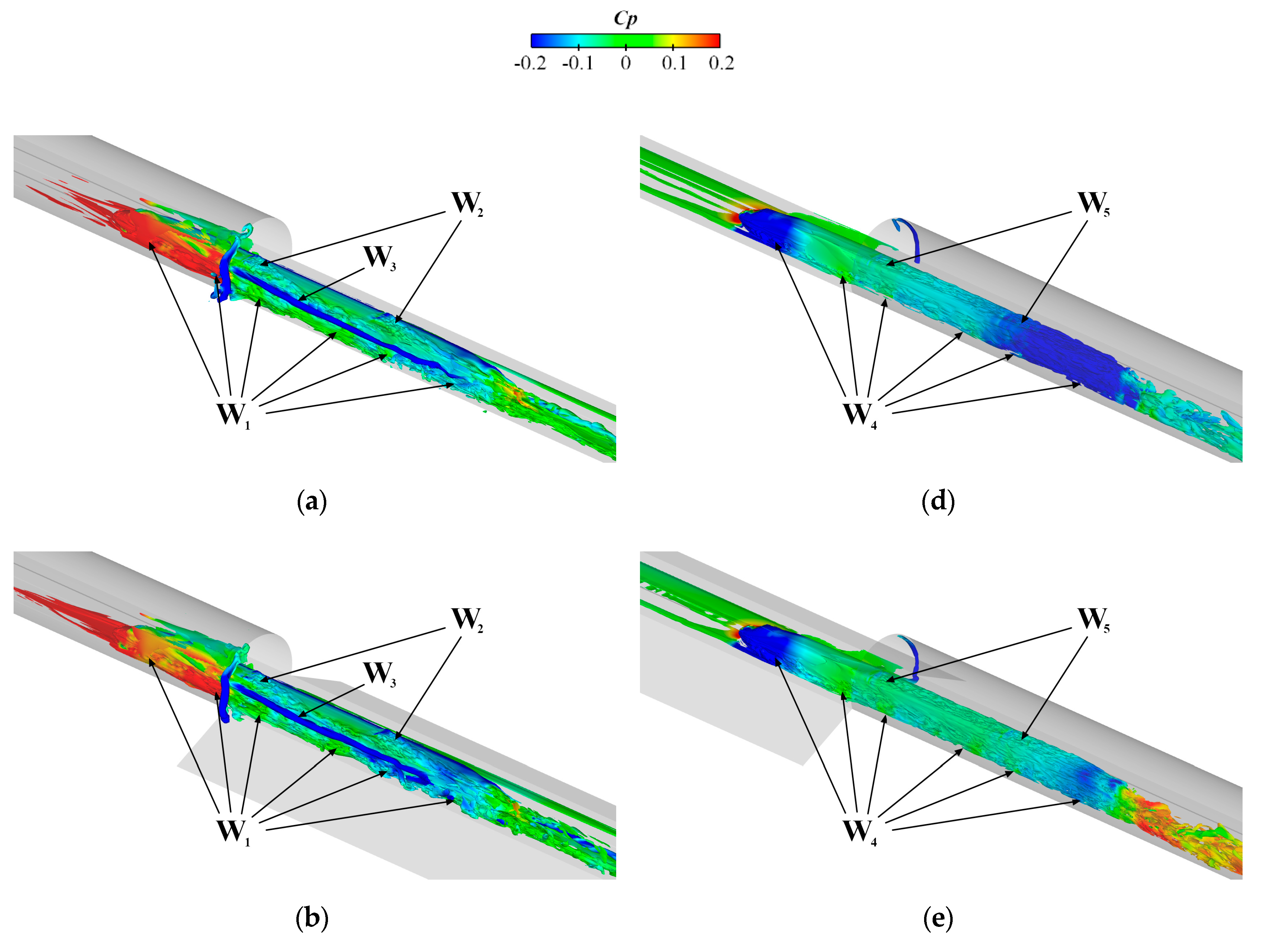
3.4. Flow Structures

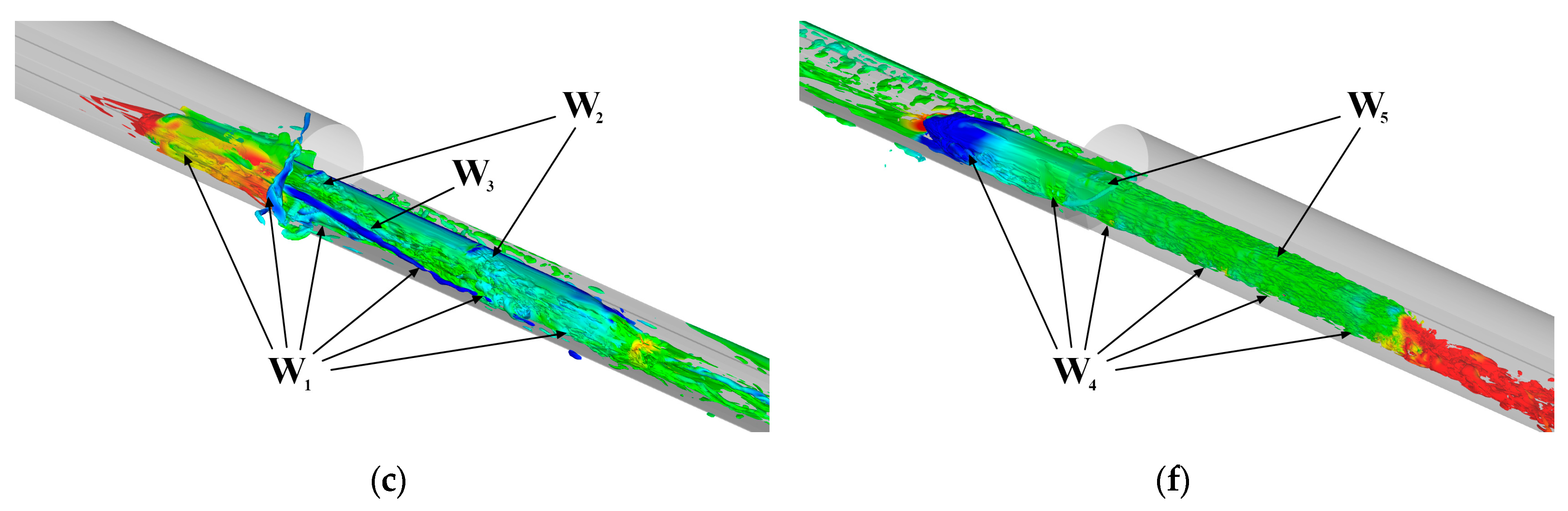
Figure 16 shows the instantaneous flow structures around the train from the leeward side of the train. The flow structures were visualized using isosurfaces of the second invariant of the velocity gradient tensor, Q = 100, colored with $C_p$. Two time instances, when the head car has just entered the tunnel (t₂) and exited into the open-air 2 region (t₆) were chosen for the flow analysis in all three cases.

Figure 16a–c show that the bogies (W₁) and inter-carriage gaps between two adjacent cars (W₂) lead to flow separations, when the train is entering the tunnel. The head car, being already in the tunnel, is covered with flow structures at high pressure; while low pressure for the structures are observed around the middle and tail cars, since they are still in the open-air 1 region. Lower pressure around the head car and higher pressure around the tail car are observed in Case 3 as compared to Case 1 and Case 2, leading to a smaller pressure difference between the three cars when the train is entering the tunnel. Note that a flow separation (W₃) with low pressure is formed from the leeward side of the head car to the tail car.

Figure 16d–f show the instants when the train is leaving the tunnel. Here, several waves are generated from the bogies (W₄) and windshields (W₅). However, these waves are smaller and denser than W₁ and W₂. The flow structures around the head car are similar, and the biggest difference among the three cases is the flow around the tail car and in the wake. The pressure of the flow structures around the tail car is lower in Case 1, as shown in Figure 16d, while the pressure in this region increases (although still negative) in Case 2, as seen in Figure 16e, and approaches 0 in Case 3 (Figure 16f). It shows that a smaller change of the flow pressure around the train is observed in Case 3.

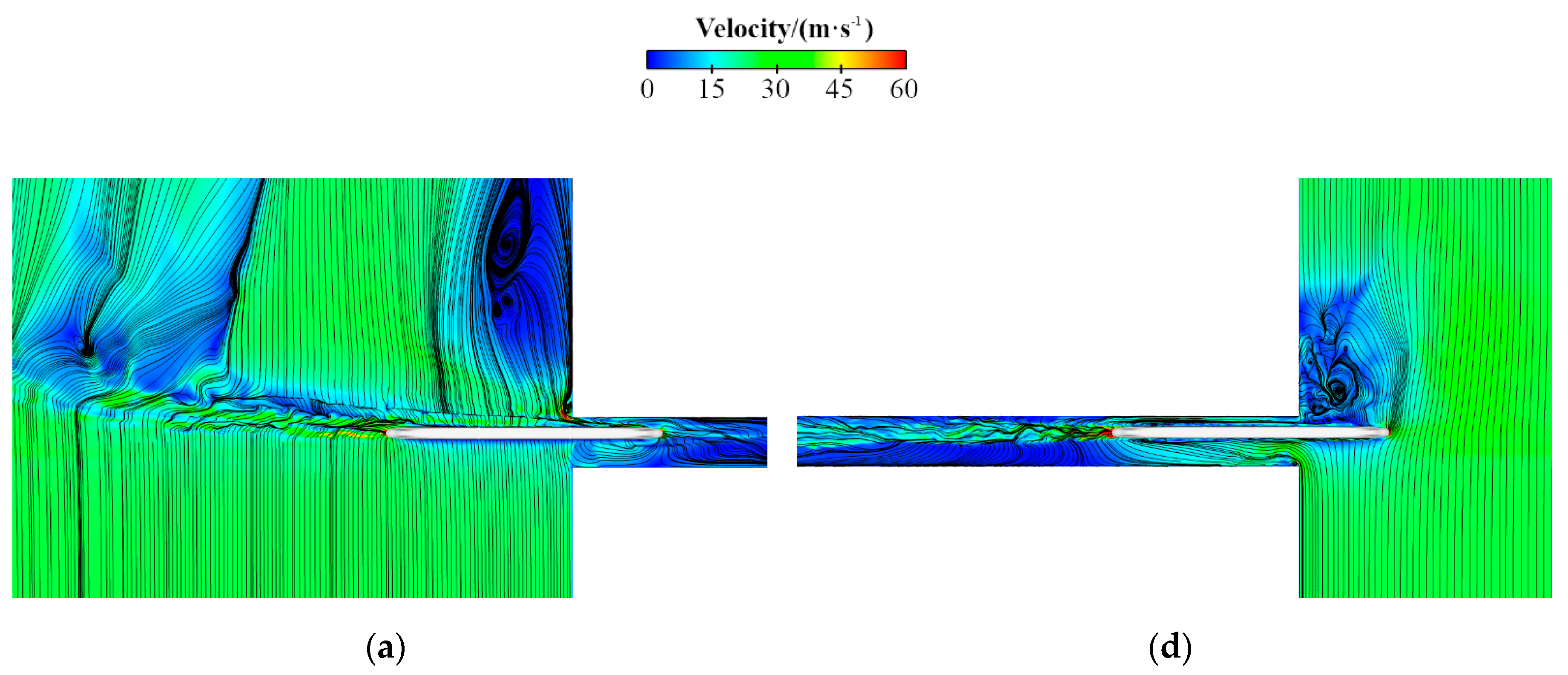
3.5. Flow Velocity

Figure 17 shows the streamlines in the horizontal plane at 1.7 m above the rail top. Two time-instances are visualized, the first one represents the moment the train is entering the tunnel, while the second, shows the exit instant. As seen in Figure 17a–c, due to the effect of the crosswind, a wake and a trailing vortex roll up from the separation on the roof of the train when the train is entering the tunnel and some parts of the train are still in the open-air region 1, which shows a reasonable agreement with the investigation of Yang [18]. Due to the blocking of the tunnel wall, the crosswind will not affect the inside of the tunnel, which means the crosswind only impinges the outside part of the train and provides a distinct lateral force on this part. Therefore, a shear force between the inside and outside parts is formed. Those regions with low and high velocities are easily to be distinguished. Two low speed regions are observed on the leeward side of the train in the region close to the junction and in the far wake. Another observation is that the two low speed zones are smaller in Case 3 than in the other two cases.

Once the train is leaving the tunnel, the head car is suddenly affected by the crosswind, resulting in flow separation and low velocity region on the leeward side of the train, as shown in Figure 17d–f. At the same time, the middle and tail cars which are still in the tunnel and only affected by the tunnel effect, which means, the flow velocity around the cars inside the tunnel is much different from the part outside the tunnel. Only the outside part of the train is suffering from the crosswind, resulting in a higher lateral force on this part, and also forming shear force between the inside and outside parts. In addition, the corresponding low speed region outside the tunnel on the leeward side of the train is smaller in Case 3 as compared to the other two cases.

4. Conclusions

This paper presents a numerical investigation of the aerodynamic performance of a high-speed train passing through different tunnel junctions under crosswind. Three ground conditions at the junction of the tunnel have been studied: A flat ground, an embankment, and a bridge configuration. This study indicates that the ground conditions outside the tunnel have significant effects on the aerodynamic performance of high-speed trains. When suffering from crosswind, the high-speed train experiences the smallest aerodynamic forces when it travels on the bridge approaching the entrance of the tunnel. In particular, the bridge case shows the lowest surface pressure on the body of the train and the tunnel, and the lowest pressure gradient at the junctions, as compared to the other two cases.

The variation of the pressure on the train body was found to be stronger on the leeward side of the train during the entrance into the tunnel and on the windward side during the exit from the tunnel. A slightly larger change in the pressure coefficient at the junction locations is observed, while the middle part of the tunnel experiences the largest peak-to-peak pressure. The integrated interaction of the moving train, the tunnel, and the crosswind results in the change of the flow field both inside and outside the tunnel. In addition, the smallest effect on the surrounding flow and its structures is observed in the bridge configuration.

The results in this study show that a bridge at the entrance and the exit of a tunnel contributes to the development of smaller aerodynamic forces. Although such a configuration is not feasible in all situations, the present study has shown the differences between three possible scenarios. This study represents a first step toward a deeper analysis of the flow at tunnel junctions. The knowledge gained from this can be used to adjust the operation of trains facing such conditions or to suggest improvements in the designing process of the junctions. Future work is now under consideration to better analyze and estimate the safety implications that different environment conditions and junction designs can bring to a high-speed train model.

References

1. Tian, H.Q. Review of research on high-speed railway aerodynamics in China. Transp. Saf. Environ. 2019, 1, 1–21. [Google Scholar] [CrossRef] [Green Version]
2. Baker, C.J. A framework for the consideration of the effects of crosswinds on trains. J. Wind Eng. Ind. Aerodyn. 2013, 123, 130–142. [Google Scholar] [CrossRef]
3. Giappino, S.; Melzi, S.; Tomasini, G. High-speed freight trains for intermodal transportation: Wind tunnel study on the aerodynamic coefficients of container wagons. J. Wind Eng. Ind. Aerodyn. 2018, 175, 111–119. [Google Scholar] [CrossRef]
4. Howe, M.S.; Iida, M.; Fukuda, T. Influence of an unvented tunnel entrance hood on the compression wave generated by a high-speed train. J. Fluids Struct. 2003, 17, 833–853. [Google Scholar] [CrossRef]
5. Yang, Q.S.; Song, J.H.; Yang, G.W. A moving model rig with a scale ratio of 1/8 for high speed train aerodynamics. J. Wind Eng. Ind. Aerodyn. 2016, 152, 50–58. [Google Scholar] [CrossRef] [Green Version]
6. Krajnović, S.; Ringqvist, P.; Nakade, K.; Basara, B. Large eddy simulation of the flow around a simplified train moving through a crosswind flow. J. Wind Eng. Ind. Aerodyn. 2012, 110, 86–99. [Google Scholar] [CrossRef]
7. He, X.H.; Zou, Y.F.; Wang, H.F.; Han, Y.; Shi, K. Aerodynamic characteristics of a trailing rail vehicles on viaduct based on still wind tunnel experiments. J. Wind Eng. Ind. Aerodyn. 2014, 135, 22–33. [Google Scholar] [CrossRef]
8. Krajnović, S. Shape optimization of high-speed trains for improved aerodynamic performance. Proc. Inst. Mech. Eng. Part F J. Rail Rapid Transit 2009, 223, 439–452. [Google Scholar] [CrossRef]
9. Hemida, H.; Baker, C. Large-eddy simulation of the flow around a freight wagon subjected to a crosswind. Comput. Fluids 2010, 39, 1944–1956. [Google Scholar] [CrossRef]
10. Hemida, H.; Krajnović, S. LES study of the influence of the nose shape and yaw angles on flow structures around trains. J. Wind Eng. Ind. Aerodyn. 2010, 98, 34–46. [Google Scholar] [CrossRef]
11. Flynn, D.; Hemida, H.; Baker, C. On the effect of crosswinds on the slipstream of a freight train and associated effects. J. Wind Eng. Ind. Aerodyn. 2016, 156, 14–28. [Google Scholar] [CrossRef] [Green Version]
12. Li, X.F.; Zhou, D.; Jia, L.R.; Yang, M.Z. Effects of yaw angle on the unsteady aerodynamic performance of the pantograph of a high-speed train under crosswind. J. Wind Eng. Ind. Aerodyn. 2018, 182, 49–60. [Google Scholar] [CrossRef]
13. Zhang, L.; Liu, H.; Stoll, N.; Thurow, K. Influence of tunnel aerodynamic effects by slope of equal-transect ring oblique tunnel portal. J. Wind Eng. Ind. Aerodyn. 2017, 169, 106–116. [Google Scholar] [CrossRef]
14. Lu, Y.B.; Wang, T.T.; Yang, M.Z.; Qian, B.S. The influence of reduced cross-section on pressure transients from high-speed trains intersecting in a tunnel. J. Wind Eng. Ind. Aerodyn. 2020. [Google Scholar] [CrossRef]
15. Niu, J.-Q.; Zhou, D.; Liu, F.; Yuan, Y.-P. Effect of train length on fluctuating aerodynamic pressure wave in tunnels and method for determining the amplitude of pressure wave on trains. Tunn. Undergr. Space Technol. 2018, 80, 277–289. [Google Scholar] [CrossRef]
16. He, K.; Gao, G.-J.; Wang, J.-B.; Fu, M.; Miao, X.-J.; Zhang, J. Performance of a turbine driven by train-induced wind in a tunnel. Tunn. Undergr. Space Technol. 2018, 82, 416–427. [Google Scholar] [CrossRef]
17. Liu, T.; Chen, Z.; Zhou, X.; Zhang, J. A CFD analysis of the aerodynamics of a highspeed train passing through a windbreak transition under crosswind. Eng. Appl. Comput. Fluid Mech. 2018, 12, 137–151. [Google Scholar]
18. Yang, W.; Deng, E.; Lei, M.; Zhang, P.; Yin, R. Flow structure and aerodynamic behavior evolution during train entering tunnel with entrance in crosswind. J. Wind Eng. Ind. Aerodyn. 2018, 175, 229–243. [Google Scholar] [CrossRef]
19. Diedrichs, B.; Sima, M.; Orellano, A.; Tengstrand, H. Crosswind stability of a high-speed train on a high embankment. Proc. Inst. Mech. Eng. Part F J. Rail Rapid Transit 2007, 221, 205–225. [Google Scholar] [CrossRef]
20. Shur, M.L.; Spalart, P.R.; Strelets, M.K.; Travin, A.K. A hybrid RANS-LES approach with delayed-DES and wall-modelled LES capabilities. Int. J. Heat Fluid Flow 2008, 29, 1638–1649. [Google Scholar] [CrossRef]
21. Menter, F.R.; Kuntz, M.; Langtry, R. Ten years of industrial experience with the SST turbulence model. Proc. Fourth Int. Symp. Turbul. Turbul. Heat Mass Transf. 2003, 4, 625–632. [Google Scholar]
22. Wang, J.B.; Minelli, G.; Zhang, Y.; Zhang, J.; Krajnovic, S.; Gao, G.J. An improved delayed detached eddy simulation study of the bogie cavity length effects on the aerodynamic performance of a high-speed train. J. Mech. Eng. Sci. 2020. [Google Scholar] [CrossRef]
23. Dong, T.Y.; Minelli, G.; Wang, J.B.; Liang, X.F.; Krajnovic, S. The effect of ground clearance on the aerodynamics of a generic high-speed train. J. Fluids Struct. 2020, 95. [Google Scholar] [CrossRef]
24. Minelli, G.; Yao, H.D.; Andersson, N.; Höstmad, P.; Forssén, J.; Krajnovic, S. An aeroacoustic study of the flow surrounding the front of a simplified ICE3 high-speed train model. Appl. Acoust. 2020, 160. [Google Scholar] [CrossRef]
25. Wang, J.B.; Minelli, G.; Dong, T.Y.; Chen, G.; Krajnovic, C. The effect of bogie fairings on the slipstream and wake flow of a high-speed train. An IDDES study. J. Wind Eng. Ind. Aerodyn. 2019, 191, 183–202. [Google Scholar] [CrossRef]
26. Dong, T.; Liang, X.; Krajnović, S.; Xiong, X.; Zhou, W. Effects of simplifying train bogies on surrounding flow and aerodynamic forces. J. Wind Eng. Ind. Aerodyn. 2019, 191, 170–182. [Google Scholar] [CrossRef]
27. Niu, J.Q.; Zhou, D.; Liang, X.F.; Liu, T.H.; Liu, S. Numerical study on the aerodynamic pressure of a metro train running between two adjacent platforms. Tunn. Undergr. Space Technol. 2017, 65, 187–199. [Google Scholar] [CrossRef]
28. Paz, C.; Suárez, E.; Gil, C. Numerical methodology for evaluating the effect of sleepers in the underbody flow of a high-speed train. J. Wind Eng. Ind. Aerodyn. 2017, 167, 140–147. [Google Scholar] [CrossRef]
29. Niu, J.Q.; Zhou, D.; Liang, X.F.; Liu, S.; Liu, T.H. Numerical simulation of the Reynolds number effect on the aerodynamic pressure in tunnels. J. Wind Eng. Ind. Aerodyn. 2018, 173, 187–198. [Google Scholar] [CrossRef]
30. British Standard. Available online: https://www.bsigroup.com/.2010EN14067-6 (accessed on 15 May 2020).
31. Cross, D.; Hughes, B.; Ingham, D.; Ma, L. A validated numerical investigation of the effects of high blockage ratio and train and tunnel length upon underground railway aerodynamics. J. Wind Eng. Ind. Aerodyn. 2015, 146, 192–206. [Google Scholar] [CrossRef] [Green Version]
Figure 1. Schematic of three junction scenarios.
Applsci 10 03664 g001
Figure 2. Models used in the calculation: (a) The CRH2 (China Railway High-speed 2) train; (b) cross-sections of the embankment, bridge, and tunnel.
Applsci 10 03664 g002
Figure 3. Sketch map of the sliding mesh.
Applsci 10 03664 g003
Figure 4. Computational domain (for Case 3).
Applsci 10 03664 g004
Figure 5. The computational mesh used in simulations: (a) Surface mesh distribution of the train, bridge and tunnel, (b) mesh distribution around the train.
Applsci 10 03664 g005
Figure 6. Schematic of measuring points locations: (a) on the middle car; (b) on the inner wall of the tunnel; (c) cross sections along the tunnel. Dimensions are in [m].
Applsci 10 03664 g006aApplsci 10 03664 g006b
Figure 7. Grid independence and time step verification: (a) Grid independence visualized by C p ; time step independence visualized by (b) C p ; (c) velocity magnitude; (d) C s .
Applsci 10 03664 g007
Figure 8. The Pingtu tunnel used for real train experiment.
Applsci 10 03664 g008
Figure 9. Comparison of the real train experiment and simulation: (a) On the train body; (b) on the inner wall of the tunnel.
Applsci 10 03664 g009
Figure 10. Curves of aerodynamic coefficients for three cars: the head car (HC), the middle car (MC), and the tail car (TC). (a) C d of HC (b) C d of MC; (c) C d of TC; (d) C s of HC; (e) C s of MC; (f) C s of TC; (g) C l of HC; (h) C l of MC; (i) C l of TC; (j) C m of HC; (k) C m of MC; (l) C m of TC.
Applsci 10 03664 g010aApplsci 10 03664 g010b
Figure 11. C p curves of the measuring points on the middle car: (a) windward side; (b) leeward side.
Applsci 10 03664 g011
Figure 12. Surface pressure distributions on the train in Case 1: (a) Entering the tunnel; (b) exiting the tunnel.
Applsci 10 03664 g012
Figure 13. C p history at monitoring points on the cross section of tunnel wall at: (a) S2; (b) S10; (c) S18.
Applsci 10 03664 g013
Figure 14. Peak to peak values of C p on the tunnel wall.
Applsci 10 03664 g014
Figure 15. Isosurface of Q = 100 coloured with C p . (a) Case 1 at t2 = 1.285 s; (b) Case 2 at t2 = 1.285 s; (c) Case 3 at t2 = 1.285 s; (d) Case 1 at t6 = 4.369 s; (e) Case 2 at t6 = 4.369 s; and (f) Case 3 at t6 = 4.369 s.
Applsci 10 03664 g015aApplsci 10 03664 g015b
Figure 16. Streamlines and velocity distributions. (a) Case 1 at t2 = 1.285 s; (b) Case 2 at t2 = 1.285 s; (c) Case 3 at t2 = 1.285 s; (d) Case 1 at t6 = 4.369 s; (e) Case 2 at t6 = 4.369 s; and (f) Case 3 at t6 = 4.369.
Applsci 10 03664 g016aApplsci 10 03664 g016b